Maize Crop Coefficient Estimation Based on Spectral Vegetation Indices and Vegetation Cover Fraction Derived from UAV-Based Multispectral Images

Abstract

Remote sensing-based crop monitoring has evolved unprecedentedly to supply multispectral imagery with high spatial-temporal resolution for the assessment of crop evapotranspiration (ETc). Several methodologies have shown a high correlation between the Vegetation Indices (VIs) and the crop coefficient (Kc). This work analyzes the estimation of the crop coefficient (Kc) as a spectral function of the product of two variables: VIs and green vegetation cover fraction (f_v). Multispectral images from experimental maize plots were classified to separate pixels into three classes (vegetation, shade and soil) using the OBIA (Object Based Image Analysis) approach. Only vegetation pixels were used to estimate the VIs and f_v variables. The spectral Kc_fv:VI models were compared with Kc based on Cumulative Growing Degree Days (CGDD) (Kc-c_GDD). The maximum average values of Normalized Difference Vegetation Index (NDVI), WDRVI, amd EVI2 indices during the growing season were 0.77, 0.21, and 1.63, respectively. The results showed that the spectral Kc_fv:VI model showed a strong linear correlation with Kc-c_GDD (R² > 0.80). The model precision increases with plant densities, and the Kc_fv:NDVI with 80,000 plants/ha had the best fitting performance (R² = 0.94 and RMSE = 0.055). The results indicate that the use of spectral models to estimate Kc based on high spatial and temporal resolution UAV-images, using only green pixels to compute VI and f_v crop variables, offers a powerful and simple tool for ETc assessment to support irrigation scheduling in agricultural areas.

1. Introduction

Crop water requirement (CWR) is the water needed to compensate for water vapour released into the atmosphere by evapotranspiration (ETc) and is one of the most critical variables in irrigated agriculture to better match water demand with irrigation supply [1]. There are several practical methodologies to estimate ETc. The most used method in the irrigation practice is well described in the FAO-56 manual [2], which is based on the knowledge of two variables: the reference evapotranspiration (ETo), representing the atmospheric evaporative demand, and the basal crop coefficient (Kcb), representing the water crop factors.

The ETo values represent the evaporative effects of environmental conditions on the evapotranspiration process and are commonly estimated by equations using weather data [3]. The Kcb coefficient is species-specific and varies according to the phenology, environmental conditions, and available soil moisture in which the crop is grown under standard conditions [4,5].

According to the FAO-56 method, Kcb values are represented by four simplified lines, which vary according to the phenological stages: seedling, vegetative growth, intermediate, and maturity. However, these Kcb values must be calibrated to local conditions [5].

Crop phenology reflects the timing of biological events, and it plays an important role in crop management to couple farm-level input demands with applications. Most models used to simulate crop development assume a linear relationship between air temperature and phenological development rate using the Growing Degree Days (GDD) concept. GDD considers the effects of temperature variation on phenology, and it has been applied successfully to improve the estimates of crop development under different weather conditions [6]. The GDD represents a thermal day index defined as the integration of the ambient temperature curve between two temperatures that define the range where crop growth occurs.

In this approach, Kcb can be expressed as a function on Cumulative Growing Degree Days (CGDD) as proposed by Ojeda-Bustamante et al. [6]. The expression of Kcb as a function of thermal time is more versatile and easier for computational implementation. However, it has the disadvantage of demanding local meteorological information and needing validation in large areas with highly spatial-temporal crop variation. Under stress conditions, Kcb is affected by water stress factors and Kcb is transformed in Kc that considers non-standard conditions [1].

Crop monitoring is required to obtain detailed information on the spatial-temporal variability of agricultural variables affecting crop canopy, the main driver of Kc. An alternative to estimating Kc is using remote sensing reflectance values to monitor crop biophysical parameters associated with crop water requirements [7,8,9].

The canopy interception of solar energy is the main driver of crop evapotranspiration. The temporal variation of sunlight interception is a direct function of leaf area. Some researchers [10,11] have reported a strong connection between Kc and canopy reflectance values at different scales. Several studies also have indicated the high correlation between vegetation biophysical characteristics and the reflectance values of spectral images [12,13].

There are many studies to estimate Kc as a function of vegetation indices (VIs) obtained from satellite images and validated with field observations [5,14,15]. The most used indices to estimate Kc are the NDVI (Normalized Difference Vegetation Index) [7,16,17,18] and the SAVI (Soil Adjusted Vegetation Index) [7,17,19,20]. Odi-Lara et al. [21] and Allen et al. [22] reported that the Kc coefficient was successfully estimated with NDVI and SAVI indices. However, NDVI and SAVI have disadvantages when correlated with some biophysical characteristics, such as crop phenology, because their relationship is non-linear. VI values can reach saturation with an asymptotic approach when the crop canopy is from moderate to high [23]. Remote sensing data are useful to characterize important agronomical variables in large areas, supported by the high crop functional correlation between the biophysical characteristics and spectral properties. Several studies show that the VIs-Kc relationship is imprecise in early phenological stages with low crop canopy [9]. Usually, spectral-based VI estimation does not separate crop canopy from the soil surface, which generates high bias under incomplete canopy cover since dark-coloured soil produces larger VI values than light-coloured soils [24].

Diverse remote sensing satellite platforms provide multispectral images to estimate vegetation indices with limited spatial resolution. Hence, a more widely used alternative is Unmanned Aerial Vehicles (UAVs) equipped with high-resolution digital cameras. Such UAVs can be deployed repeatedly, at low cost, with greater flexibility in altitude and higher spatial and temporal resolutions [25]. The use of UAVs for agricultural monitoring has multiplied in recent years [26] thanks to the smaller size and lower cost of multispectral and thermal cameras [27]. However, VIs generated from multispectral images of high spatial resolution require validation at a local scale to estimate the Kc spatial variation with good precision [18].

Green Vegetation Cover Fraction (f_v) has also been used for studying the phenological and physiological status of vegetation [28], estimating crop yields and monitoring crop developmental stages [29]. Marcial-Pablo et al. [30] showed that f_v could be estimated with precision from VI indices from UAV-based RGB and multispectral images. Since VIs and f_v are correlated with crop phenology and crop canopy density, it is necessary to study their correlation with Kc. Johnson and Trout [31] reported that Kc can be estimated based on f_v indices with the support of vegetation indexes. Several authors reported a strong relation of f_v and VIs with biophysical variables such as Fraction of Absorbed Photosynthetically Active Radiation (fAPAR), an important variable in the agricultural monitoring [32,33].

ETc estimation has focused on standardized crop conditions and full irrigation conditions [34]. There are very robust methodologies to estimate Kcb based on thermal time expressed as a continuous function of Cumulative Growing Degree Days (CGDD) reported by Ojeda-Bustamante et al. [6]. CGDD-based functions are considered a suitable option to account for the climate variability on crop growth and phenological development. However, Kc under non-standard conditions is important to know for crops with highly-variable water demands. For better water planning and management, and given the limited meteorological information in many agricultural zones, it is necessary to use geospatial technologies to indirectly estimate crop water demands. Remote sensing data have been used to assess water stress in non-standard conditions of various crops using low resolution such as satellites images and high resolution (UAV) imagery [18].

The existing research has been concentrated on using spectral data to estimate crop coefficient (Kc) based mainly on a linear relationship either with the vegetation index or with vegetation cover fraction. However, with the availability of high spatial and temporal resolution images and better image analysis algorithms, it is now better to split and classify pixels of vegetation, shadow, and soil and isolate their effects and result in better spectral models to fit experimental Kc data.

Therefore, the purpose of this paper was to estimate the maize crop coefficient (Kc) as a function of the product of spectral vegetation indices (VIs) and Vegetation Cover Fraction (f_v), using high-resolution multispectral UAV-images and an efficient OBIA-based approach to classify image pixels. The proposed methodology was validated using Kc, estimated with a Cumulative Growing Degree Days (CGDD) approach, and gathered experimental data with two planting densities.

2. Materials and Methods

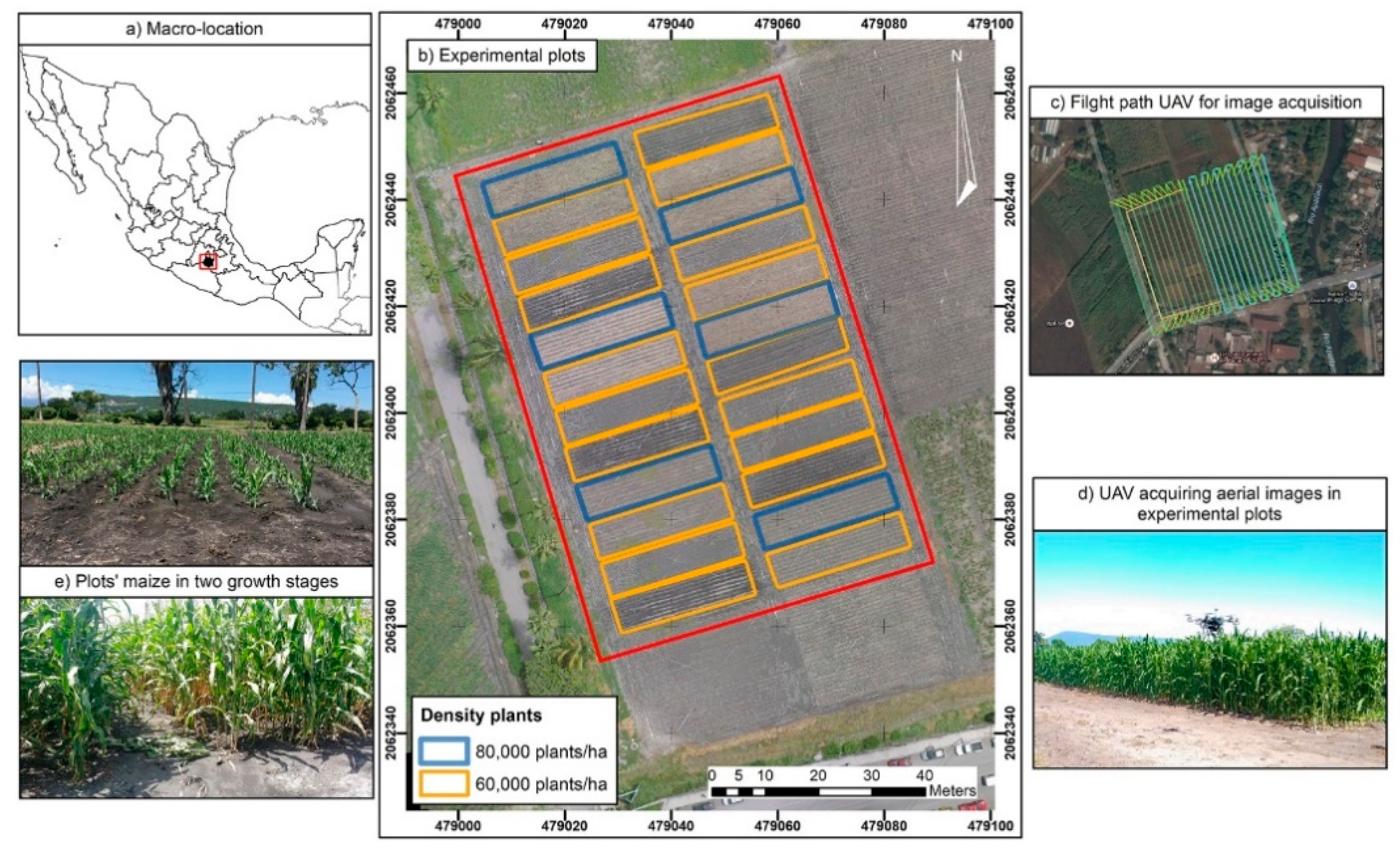
2.1. Study Area and Site Data

The field study was conducted in the experimental station (Figure 1) of the National Institute of Forestry, Agriculture and Livestock Research (INIFAP) in Zacatepec, in the Southern State of Morelos, Mexico (18° 39′ 6.45″ N and 99° 11′ 59.63″ W). The climate in the study area is hot sub-humid, with average annual temperature and precipitation of 24.3 °C and 892 mm, respectively; the rainy season is from mid-May to October, and the dry season, November to mid-May.

The experimental cropped area was 1 ha, sowed with maize hybrid H-515 on 5 July 2016. Twenty-four lots of 6 m × 25 m were planted with a furrows’ separation of 0.8 m at two plant densities (60,000 and 80,000 plants/ha). The volumetric field capacity (FC) and permanent wilting point (PWP) soil water content were 41% and 22.5%, respectively. Weather daily data were available from a meteorological station located at 160 m of the study area (18° 39′ 11.19″ N and 99°12′ 00.47″ S).

2.2. Crop Evapotranspiration (ETc)

Crop Evapotranspiration (ETc) is rarely measured in the field and is usually estimated by multiplying the reference evapotranspiration (ETo) with a crop coefficient (Kc) [1,2,6].

$$\mathrm{ETc}=\mathrm{Kc}\times \mathrm{ETo}$$

(1)

Many equations have been developed to estimate ETo and extensively evaluated and compared with measured lysimeter ET under different climatic conditions. However, the FAO Penman--Monteith method is reliable and physically-based and adopted as the standard method for ETo computation [1,2]. With data registered in weather stations, the PM method estimates ETo as a function of net radiation, soil heat flux, wind speed, air temperatures, vapour pressure, and other coefficients as described in Allen et al. [1].

The crop coefficient Kc is a crop-specific coefficient representing the physical and physiological differences between a specific crop and the reference crop, considering the relationship between the atmosphere, crop physiology, and agricultural practices [1,2,15]. Kc values for annual crops increase from a minimum value at planting until reaching a maximum value at full canopy cover. One of the main limitations of this approach is to generate specific Kc values instead of using the general FAO Kc curves supplied by Allen et al. [1].

2.3. Estimation of GDD-Based Crop Coefficient (Kc)

Under water stress conditions and neglecting soil water evaporation, the crop coefficient (Kc) can be estimated using the following equation [1]:

$$\mathrm{Kc}=\mathrm{Kcb}\times \mathrm{Ks}$$

(2)

Kcb is the basal crop coefficient obtained under optimal crop development conditions, and Ks is the soil’s water stress coefficient. Kcb was estimated using a GDD-based approach with Equation (3) proposed by Ojeda-Bustamante et al. [6], as a function of the cumulative Growing Degree Days (x_n) to day i.

$${\mathrm{Kcb}}_i={\mathrm{K}}_{\max }\mathrm{erfc}\left({\left(\frac{{\mathrm{x}}_i-{\mathrm{x}}_{{\mathrm{K}}_{\max }}}{{\mathsf{\alpha }}_1}\right)}^2\right);\mathrm{If}\mathrm{Kc}<{\mathrm{Kc}}_0,\mathrm{then}\mathrm{Kc}={\mathrm{Kc}}_0$$

(3)

Kc₀ is the basal crop coefficient for the first phenological stage that depends essentially on soil evaporation; K_max is the maximum value of the basal crop coefficient (Kcb) during the growing period; erfc is the complement error function; x_i is the cumulative Growing Degree Days (CGDD_i) elapsed until the day i from sowing or crop emergence, normalized to the maximum CGDD value required to complete the phenological cycle (CGDD_x), i.e., x_i = CGDD_i/CGDD_x; x_Kmax is the normalized dimensionless value x when the maximum value K_max is reached; α₁ is the regression coefficient obtained from fitting the model to the experimental data.

The Cumulative Growing Degree Days (CGDD) are calculated as the accumulated daily Degree Days (GDD) according to the following Equation (4) used by Ojeda-Bustamante et al. [6].

$$\begin{gathered} {\mathrm{GDD}}_i={\mathrm{T}}_{\mathrm{a}}-{\mathrm{T}}_{\mathrm{c}-\min },{\mathrm{T}}_{\mathrm{a}}<{\mathrm{T}}_{\mathrm{c}-\max } \\ {\mathrm{GDD}}_i={\mathrm{T}}_{\mathrm{c}-\max }-{\mathrm{T}}_{\mathrm{c}-\min },{\mathrm{T}}_{\mathrm{a}}\ge {\mathrm{T}}_{\mathrm{c}-\max } \\ {\mathrm{GDD}}_i=0,{\mathrm{T}}_{\mathrm{a}}\le {\mathrm{T}}_{\mathrm{c}-\min } \end{gathered}$$

(4)

${\mathrm{T}}_{\mathrm{a}}$ is the average daily air temperature, ${\mathrm{T}}_{\mathrm{c}-\min }$ and ${\mathrm{T}}_{\mathrm{c}-\max }$ are the basal (10 °C) and maximum (30 °C) growing temperatures for maize [35]. The stress adjusted crop coefficient of the day i (Ks_i) was determined as a function of the available soil water for day i (AW_i) as used by Jensen et al. [36]:

$${\mathrm{Ks}}_i=\frac{\ln \left({\mathrm{AW}}_i+1\right)}{\ln \left(101\right)}$$

(5)

Ojeda-Bustamante et al. [37] calibrated and validated the above equations for fully irrigated maize with a planting density of 95,000 plants/ha, obtaining the following parameters: K_max = 1.25, Kc₀ = 0.2, X_Kmax = 0.59. In our study, for plant densities of 60,000 and 80,000, the K_max values were estimated at 1.03 and 1.10, respectively.

Daily values of Kc were estimated using the methodology and information validated for the study area as reported by Ojeda-Bustamante et al. [6] and adjusted under field conditions considering the experiment’s planting densities.

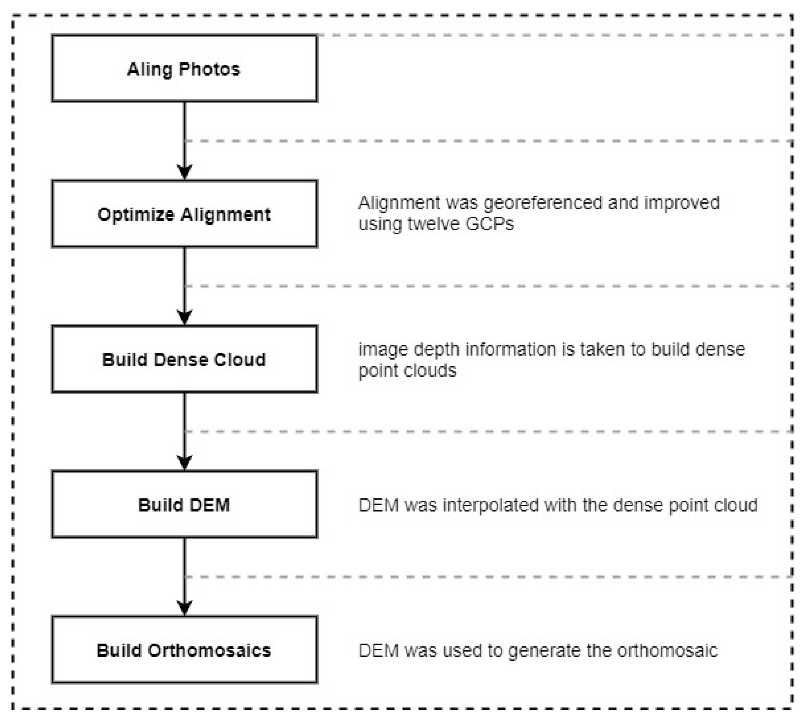
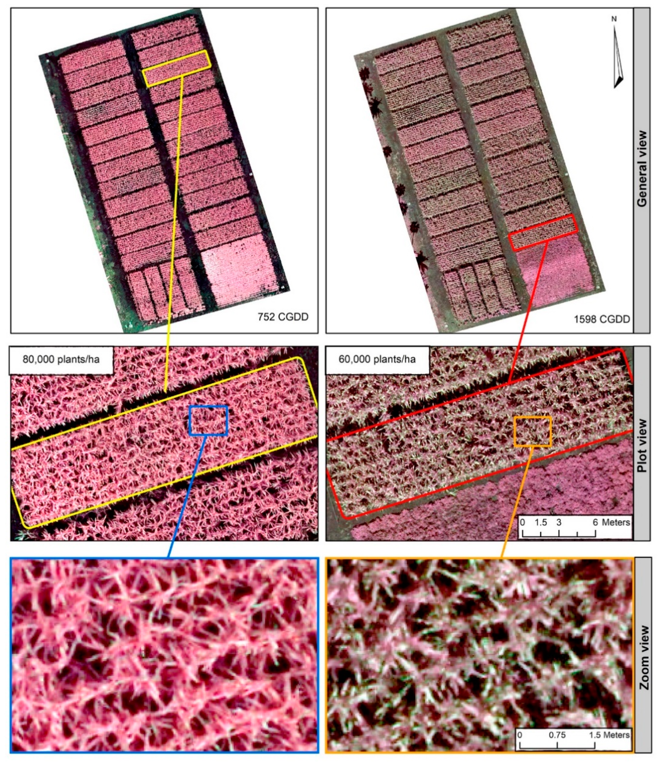
2.4. UAV Multispectral Image Acquisition and Orthomosaic Generation

UAV multispectral images were acquired during the growing season as described as follows. Twelve Ground Control Points (GCPs) evenly distributed over the study area were placed and georeferenced with a TopCon model GR-5 GPS RTK with a vertical and horizontal accuracy of <1 cm. The hexacopter UAV used was a DJI A2 model (equipped with IMU) with a maximum load capacity of 2.5 kg and top ascent and descent speed of 6 m/s. The UAV was equipped with Tetracam ADC Snap (Tetracam Inc. Chatsworth, CA, USA) three-band multispectral camera (

Table 1. UAV camera specifications.

Characteristics	Description
Imaging sensor	Tetracam ADC Snap
Sensor Type	CMOS global shutter
Sensor size (mm)	6.59 × 4.9
Resolution (pixels)	1280 × 1024 (1.3 Mp)
Focal length(mm)	8.43
Spectral bands	G: green (520–600 nm)
	R: red (630–690 nm)
	NIR: near-infrared (760–900 nm)
Dimensions (mm)	75 × 59 × 33
Weight (g)	90

).

Two flights (Figure 1c) were made on six different dates (from August to October, 2016, between 11:00 and 13:00 local time). The effective flight time for each date was 11 min and the average flight height was 50 m above the ground (GSD = 2.1 cm/pixel). Image overlap was 75% (front and side overlap) (

Table 2. Description of flight characteristics for image acquisition.

No.	Acquisition Date	Flight Local Time	Wind Speed (m/s)	Temperature (°C)
1	26 August	13:00	1.1	29.0
2	15 September	12:00	0.8	28.0
3	28 September	12:00	1.0	25.5
4	6 October	12:00	1.0	26.0
5	13 October	11:00	1.1	23.5
6	26 October	12:00	1.1	24.5

). The flights were planned and executed during the clear sky condition with the UgCS software (SPH Engineering, Riga, Latvia).

RAW images acquired by the sensor are then radiometrically calibrated in post-processing using PixelWrench2 software, thanks to a calibration target (spectralon) acquired before each flight. The digital elevation model and orthomosaic were generated using Pix4D software (Pix4D SA, Prilly, Switzerland) as shown in the Figure 2. Figure 3 shows as example, two multispectral orthomosaics obtained from photogrammetric processing of UAV images at the phenological stages.

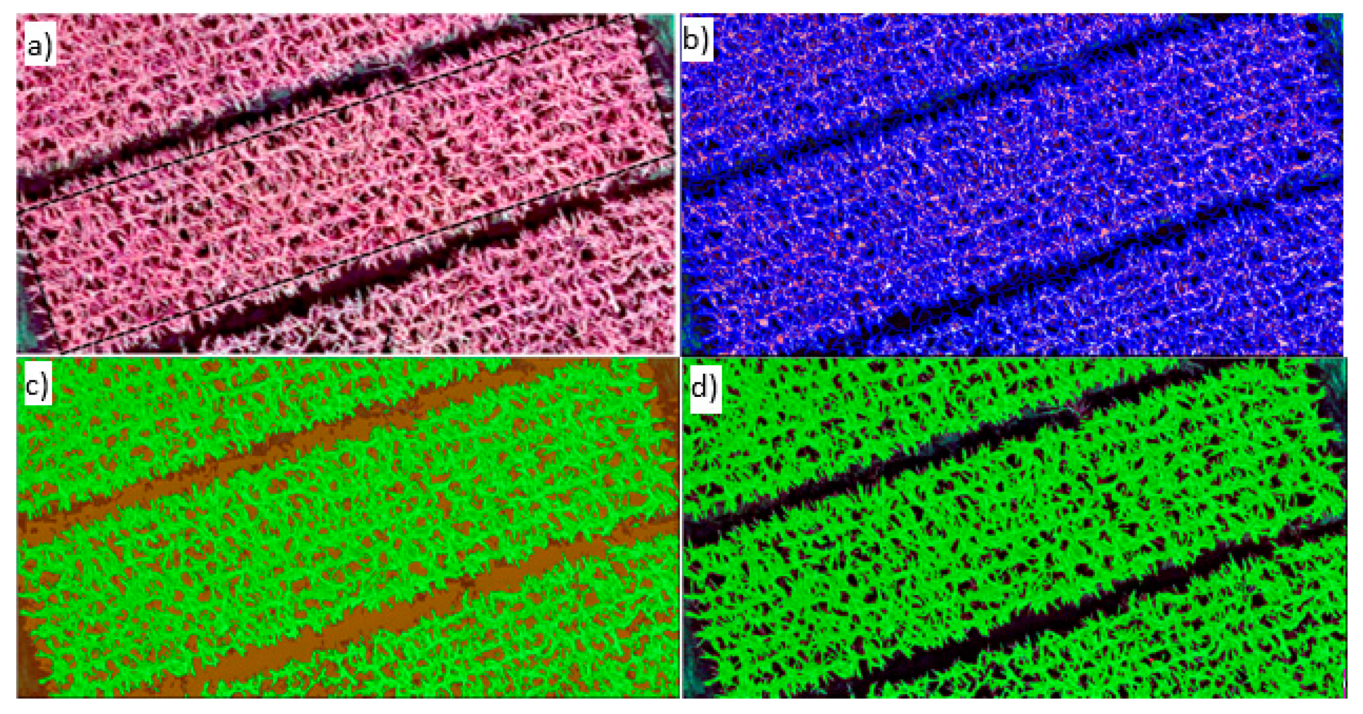
2.5. Image Classification and Estimation of GreEN Vegetation Cover Fraction (f_v)

The classification of orthomosaics was performed using the OBIA approach. The OBIA detectors were implemented using eCognition developer 9.0 (Trimble GeoSpatial, Munich, Germany). OBIA combines spectral, contextual, and morphological information of the objects created in the segmentation [39] and minimizes the average heterogeneity of the objects in the image [40]. Several papers show the successful use of this methodology to analyze high-resolution spatial images taken with UAV [41,42,43].

Two stages are involved in an OBIA approach: image segmentation and classification. Orthomosaics was segmented using the multi-resolution segmentation (MRS) algorithm that use three criteria (scale, shape, and compactness) to generate the segments. The values of the final configuration for the scale parameter, shape, and compactness were: 25, 0.3, and 0.5, respectively, as proposed by Drǎguţ et al. [44] and Drǎguţ et al. [45]. The output of this step produced homogeneous segments of different sizes.

Finally, the classifications with three classes (vegetation, shadow, and soil) were based on the segments generated (Figure 4). The method described by Marcial-Pablo et al. [30] was adapted to classify the orthomosaic into three classes.

In this way, f_v values are only estimated on vegetation pixels. The f_v values for each plot were obtained by the following equation.

f_v = Number of vegetation pixels/Number of (vegetation + non-vegetation) pixels

(6)

2.6. Estimation Vegetation Indices

There is a vast repository of vegetation indices used to explain vegetation characteristics related to ET. NDVI is probably the most widely used spectral index. However, in studies with satellite imagery, it can be affected by changes in soil background brightness and atmospheric effects caused by scattering and absorption by aerosols. In this study the use of UAV imagery can overcome these limitations. VIs such as EVI2 and WDRVI, improved versions of EVI and RDVI, offer better results by overcoming the absence of a blue band or the non-linear relationship with LAI or VF in satellite images. However, so far, these indices have been little studied in UAV images.

Table 3. Vegetation indices calculated for UAV orthomosaic images.

VIs	Abbreviation	Equation	Reference
Normalized Difference Vegetation Index	NDVI	$\frac{\mathrm{NIR}-\mathrm{R}}{\mathrm{NIR}+\mathrm{R}}$	[46]
Wide Dynamic Range Vegetation Index	WDRVI	$\frac{\mathsf{\alpha }\mathrm{NIR}-\mathrm{R}}{\mathsf{\alpha }\mathrm{NIR}+\mathrm{R}}$	[47]
2-band Enhanced Vegetation Index	EVI2	$2.5\left(\frac{\mathrm{NIR}-\mathrm{R}}{\mathrm{NIR}+2.4\mathrm{R}+1}\right)$	[48]

Note: α is weighting coefficient of 0.2 according to [47].

shows the VIs calculated for the six segmented multispectral orthomosaics using the QGIS software. VIs was estimated using two cases: using all pixels and using vegetation pixels only. A Tukey’s mean test (p ≤ 0.10) was used to analyze if there were significant differences between VIs value obtained from Case 1 and Case 2.

Increasing positive NDVI values indicate increasing amounts of green vegetation [49] because healthy vegetation has a low reflectance of red light and high reflectance of near-infrared, which results in high NDVI values. NDVI is closely related to biophysical vegetation parameters, such as LAI, but has the drawback that it loses sensitivity to change when it reaches a threshold and becomes saturated. This saturation is because chlorophyll is a very efficient absorber of red radiation, and therefore, as plant biomass increases, red reflectance will not change. On the other hand, several spectral indices such as WDRVI and EVI2 are suitable in UAV imagery without the saturation limitation [50].

WDRVI shows greater sensitivity to changes in leaf area index (LAI) values from moderate to high (between 2 and 6) than the NDVI and maintains a linear relationship with the LAI of maize and soybeans [47,51].

EVI2 considers two bands of the enhanced vegetation index (EVI); it has been developed for sensors without a blue band. Besides, similar to EVI, it maintains improved sensitivity and linearity in high biomass and LAI regions [52]. EVI2 captures spatial-temporal variation in photosynthetically active vegetation [48] and is less prone to saturation in dense vegetation cover and less sensitive to different soil reflectances [53]. EVI2 is better than NDVI at discriminating land cover diversity [54] and capturing vegetation condition and structure changes [53]. However, the seasonal variation of EVI2 in arid and semi-arid zones is not as strong as in the NDVI [55]. The three spectral vegetation indices’ values (VIs) were normalized to a scale of 0 to 1 for equally and better comparison.

2.7. Estimation Crop Coefficient Based f_v:VIs (Kc_fv:VI)

Several studies demonstrate that the use of spectral vegetation indices from near-infrared (NIR) and visible regions has a linear correlation with the interception of sunlight from the canopy [56,57]. Kc obtained from vegetation indices are more robust than assuming standard conditions (Kcb) since they estimate current crop conditions [34]. Since high VI values indicate plant areas under optimal conditions, it was assumed that the model Kc = f(f_v × VIs) is better than the simpler model Kc = f(VIs) used in most studies [11,34]. Therefore, Kc has been estimated as a function of two independent relationships: Kc = f(VIs) and Kc = f(f_v), as reported by Johnson and Trout [31]. Moreover, direct estimation of Kcb has been documented by Pôças et al. [15] using sophisticated equations as a function of f_v and VIs. Vegetation Cover Fraction (f_v) describes a vertical projection of the areal proportion of a landscape occupied by green vegetation [58]. Grattan et al. [59] and Pôças et al. [15] have reported a strong correlation between f_v and Kc.

Kc based on VIs and f_v was estimated using the following equation:

(green pixels only, using VIs and f_v): Kc_fv:VIs = a + b ∗ (f_v ∗ VIs)_{Vegetation pixels}

(7)

where a and b are fitting parameters between CGDD-based Kc data and predicted data by the three models.

Evaluation of Model Performance

Predicted (Kc_fv:VIs) and observed Kc-c_GDD values were compared using correlation analysis and linear regression (including 95% confidence prediction intervals). Several statistical parameters were calculated, mean square error (MSE), root mean square error (RMSE), mean absolute error (MAE), efficiency (E), and coefficient of variation (CV), to assess the performance of the regression model, using the equations (8 to 12) [60,61].

$$\mathrm{CME}=\frac{{\sum }_{i=1}^{\mathrm{n}}{\left({\mathrm{O}}_i-{\mathrm{P}}_i\right)}^2}{\mathrm{n}}$$

(8)

$$\mathrm{RMSE}=\sqrt{\frac{{\sum }_{i=1}^{\mathrm{n}}{\left({\mathrm{O}}_i-{\mathrm{P}}_i\right)}^2}{\mathrm{n}}}$$

(9)

$$\mathrm{MAE}=\frac{{\sum }_{i=1}^{\mathrm{n}}\left|{\mathrm{O}}_i-{\mathrm{P}}_i\right|}{\mathrm{n}}$$

(10)

$$\mathrm{E}=1-\frac{{\sum }_{i=1}^{\mathrm{n}}{\left({\mathrm{O}}_i-{\mathrm{P}}_i\right)}^2}{{\sum }_{i=1}^{\mathrm{n}}{\left({\mathrm{O}}_i-{\mathrm{O}}_{\mathrm{m}}\right)}^2}$$

(11)

$$\mathrm{CV}=\frac{\mathrm{RMSE} }{{\mathrm{O}}_{\mathrm{m}}}\times 100$$

(12)

O_i are the observed values (Kc-c_GDD), P_i are the predicted values Kc_fv:VI, O_m is the mean observed value, and n is the total number of samples.

3. Results and Discussion

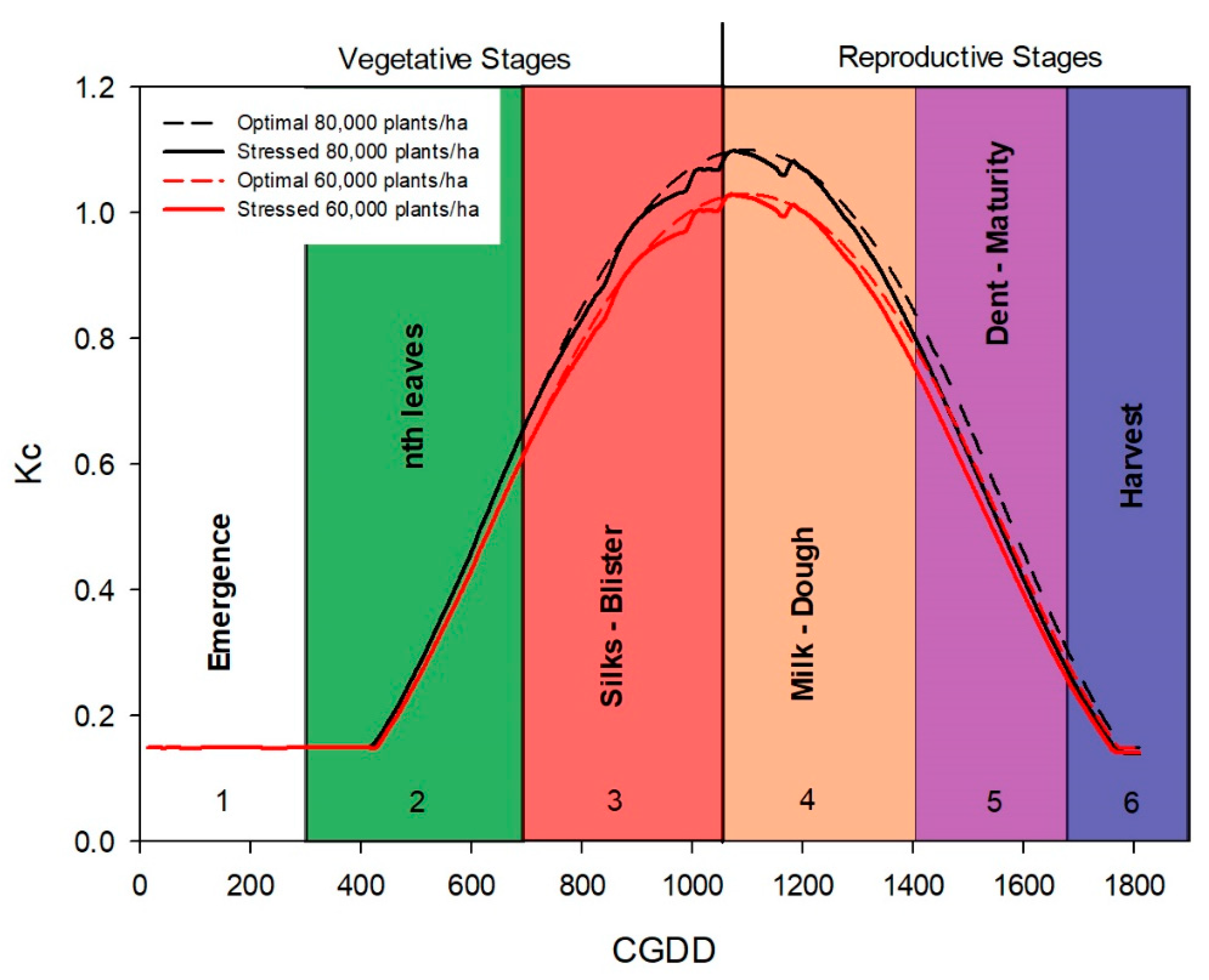
3.1. Maize Crop Coefficient CGDD-Based (Kc-c_GDD)

The maize phenological duration was 119 days (from planting to physiological maturity), equivalent to 1655 GDDs. The Kc values are detailed in

Table 4. Estimated crop coefficient values (Kc-c_GDD) for phenological stages and two density plants.

ID	Phenological Stages	Kc-cGDD		CGDD
		80,000 Plants/ha	60,000 Plants/ha
1	Planting—2 leaves	0.15	0.15	300
2	2–12 leaves	0.15–1	0.15–0.93	300 a 700
3	Silk—Blister	1.00–1.15	0.93–1.03	700 a 1050
4	Milk—Dough	1.10–0.4	1.03–0.370	1050 a 1400
5	Dent—Maturity	0.4–0.3	0.37–0.28	1400 a 1650
6	Harvest	0.3–0.18	0.28–0.2	>1650

and Figure 5, which shows that the peak Kc values are in the blister-milk stages.

The simulated Kc values (Figure 5), for both plan densities, show good agreement between the optimal (Kcb) and stressed (Kc) curve, indicating a good match between crop water demands and rainfall, with small differences during blister and milk stages. As expected, Kc values are higher for higher plant density (80,000 plants/ha) because of the higher vegetation coverage due to high crop biomass.

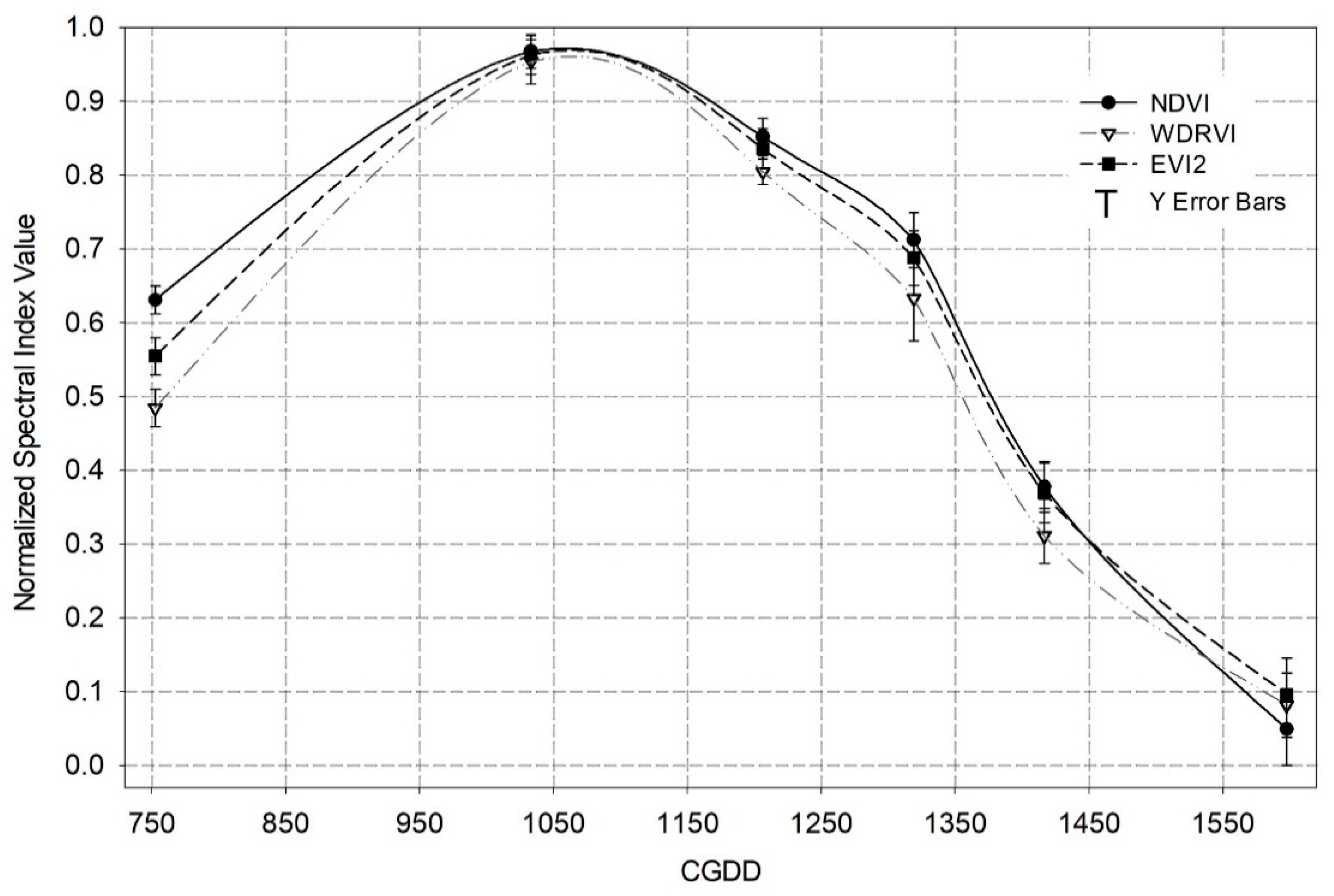
3.2. Vegetation Indices (VIs)—CGDD Relationship

A Tukey HSD test (p ≤ 0.10) reflected that there are statistically significant differences between VIs values obtained from case 1 (considering three classes) and for case 2 (considering one class) (RMSE = 0.66; p = 0.00) mainly due to the effect when considering shade and soil pixels [62]. This difference is not detectable at larger spatial resolutions, as in satellite images, where pixel disaggregating is not possible. In that sense, case 2 was used in this work because it has better results and better represents the characteristics of the vegetation in the field.

The normalized values of NDVI, WDRVI, and EVI2 vegetation indices obtained for case 2, using only vegetation pixels of the all plots (two densities plants), are compared with the cumulative GDD values calculated for the day of flights (Figure 6). The normalized values of average VIs range from 0.45–0.60 (750 CGDD) in the early stages, 0.93–0.98 (1033 CGDD) in silks, 0.78–0.88 (1206 CGDD) in milk stage, 0.27–0.76 (1319 to 1417 CGDD) in dough-dent grain stages, and 0–0.15 (>1550 CGDD) in the maturity stage, with an average standard deviation between 0.01 to 0.03 for all stages. In this work, the VIs values show more variability in the maturity stages by leaf moisture and colour changes, which coincides with Xin et al. [63]. Besides, our results show that the VIs tends to decline after a full cover is reached in the crop season, similar to Kc [4].

The results are comparable to those reported by Calera et al. [64], who obtained NDVI values between 0.10 and 0.85 (with a peak at flowering) using Landsat 7 images. Also by Gitelson et al. [65], who found NDVI values from 0.28 to 0.85 for vegetative and reproductive stages, respectively, using MODIS images, and by Raun et al. [66] with peak NDVI values (0.77 to 0.73) at flowering, estimated with a Greenseeker sensor.

Most remarkable differences between NDVI, EVI2, and WDRVI occurred in the early and late stages, where EVI2 and WDRVI are more sensitive to vegetation changes than NDVI. In this regard, Guzinski [67] reports that although the three indices were useful for estimating crop phenology, there are differences between them when the crop canopy density changes drastically in the early and late stages.

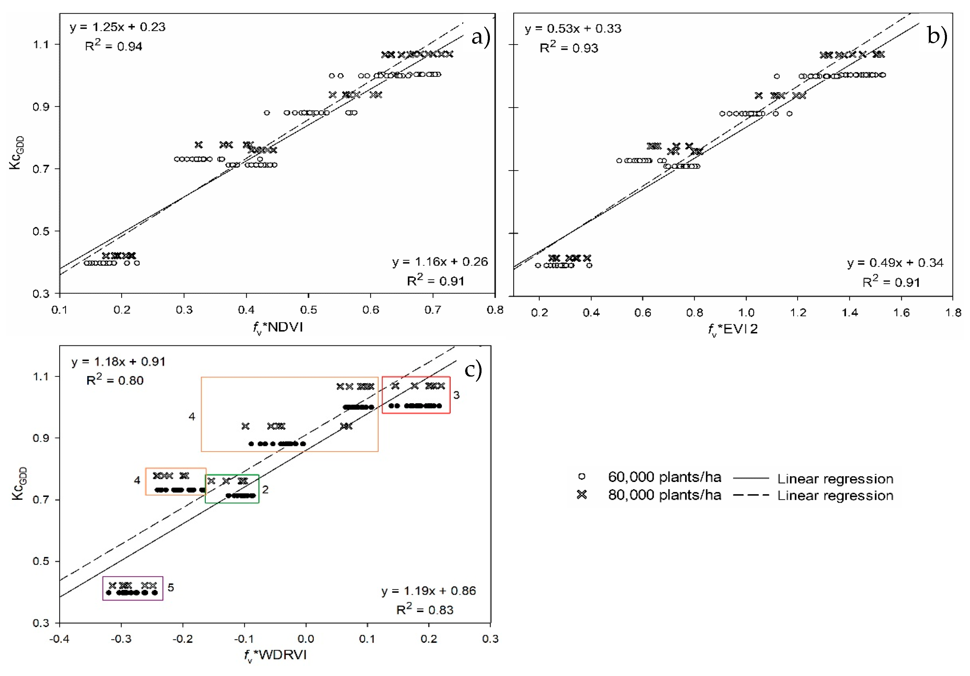
3.3. f_v:VIs Approach for Kc Estimation

The high spatial resolution of UAV imagery, as calculated for case 2, improves the accuracy of clustering, detection, and classification of pixel classes and thus increases the ability to recognize vegetation characteristics from vegetation indices. A strong linear correlation (R² > 0.8) between VIs from green vegetation pixels and Kc-c_GDD values was found in the study. Therefore, considering both f_v and NDVI improved the Kc(f_v:NDVI) prediction, since f_v is an expression of “only-green” biomass coverage and NDVI estimates the greenness “quality”. Both variables are related with canopy photosynthetic activity, and non-green pixels should be not considered, since they are associated with shadow soil and decay leaves.

It is interesting to note that the fitting model accuracy (model vs observed Kc-c_GDD data) increases with plant density due to high canopy density, improve the correlation for the case of NDVI (R² > 0.91), while they do not change for EVI2 and decrease for WDRVI (R² > 0.8). Furthermore, all VIs were less sensitive to detect Kc changes because of reduced canopy density in the final stages (maturity in 1598 CGDD). On the other hand, these results show that the f_v: NDVI and f_v: EVI2 models disaggregate the vegetation canopy cover from the soil more effectively than f_v WDRVI at vegetative stages (12 leaves).

Table 5. Statistical parameters resulting from Kc_fv:VIs model fitting using observed Kc-CGDD data.

fv:VI Model	CGDD	Mean	Max	Min	STD	Fitting Parameters (fv:VIs)
						80,000 Plants/ha			60,000 Plants/ha
						a	b	R2	a	b	R2
fv:NDVI	752	0.59	0.62	0.53	0.02	1.25	0.23	0.94	1.16	0.26	0.91
	1033	0.76	0.80	0.71	0.02
	1206	0.7	0.74	0.64	0.02
	1319	0.63	0.67	0.55	0.03
	1417	0.46	0.51	0.41	0.03
	1598	0.3	0.37	0.23	0.03
fv:EVI2	752	1.08	1.12	0.98	0.03	0.53	0.33	0.93	0.49	0.34	0.91
	1033	1.63	1.68	1.54	0.03
	1206	1.46	1.5	1.36	0.04
	1319	1.26	1.34	1.14	0.05
	1417	0.84	0.93	0.72	0.05
	1598	0.48	0.62	0.35	0.06
fv:WDRVI	752	−0.15	−0.13	−0.21	0.02	1.18	0.91	0.80	1.19	0.86	0.83
	1033	0.21	0.24	0.15	0.02
	1206	0.09	0.12	0.06	0.01
	1319	−0.04	0.08	−0.11	0.04
	1417	−0.28	−0.23	−0.35	0.03
	1598	−0.46	−0.39	−0.52	0.03

and Figure 7 shows the statistical parameters and the linear regression between Kc-c_GDD values and VIs multiplied by f_v value (f_v:NDVI, f_v:EVI2, and f_v:WGRDI). A strong linear correlation with an R² coefficient greater than 0. 80 for all cases is observed. The model precision is high R² values about 0.94 (Figure 6), indicating that VIs values are sensitive to canopy density, associated with planting densities [68]. Besides, in early stages with low levels of canopy cover, the relationship of reflectance levels with Kc values is not very clear, due to higher variation on soil spectral properties [9]. On the other hand, the Kc_fv:NDVI model (R² = 0.94) is more sensitive to vegetation cover change than Kc_fv:EVI2 (R² = 0.80) and Kc_fv:WDRVI (R² = 0.93) due to a reduction of the saturation of the NDVI when leaf cover reaches high levels.

Similar works have reported lower R² values with satellite images, Spiliotopoulos & Loukas [69] obtained an R² of 0.86 of the Kc-EVI2 relationship from Landsat 7 ETM images. Kamble et al. [4] calculated Kc values from MODIS imagery using a simple linear regression model Kc_-NDVI with an R² of 0.83. Gitelson [47] recommended WDRVI to estimate canopy cover from Landsat images with higher accuracy than NDVI.

Furthermore, all VIs were less sensitive to detect Kc changes because of reduced canopy density in the final stages (Maturity in 1598 CGDD). On the other hand, these results show that the f_v: NDVI and f_v: EVI2 models disaggregate the vegetation canopy cover from the soil more effectively than f_v WDRVI at vegetative stages (12 leaves).

In this study, there are no images of the early growth stages of the crop because the canopy cover of the crop has a minimal effect on evapotranspiration; however, it could be interesting in future studies to monitor the crop periodically from the beginning of plant development.

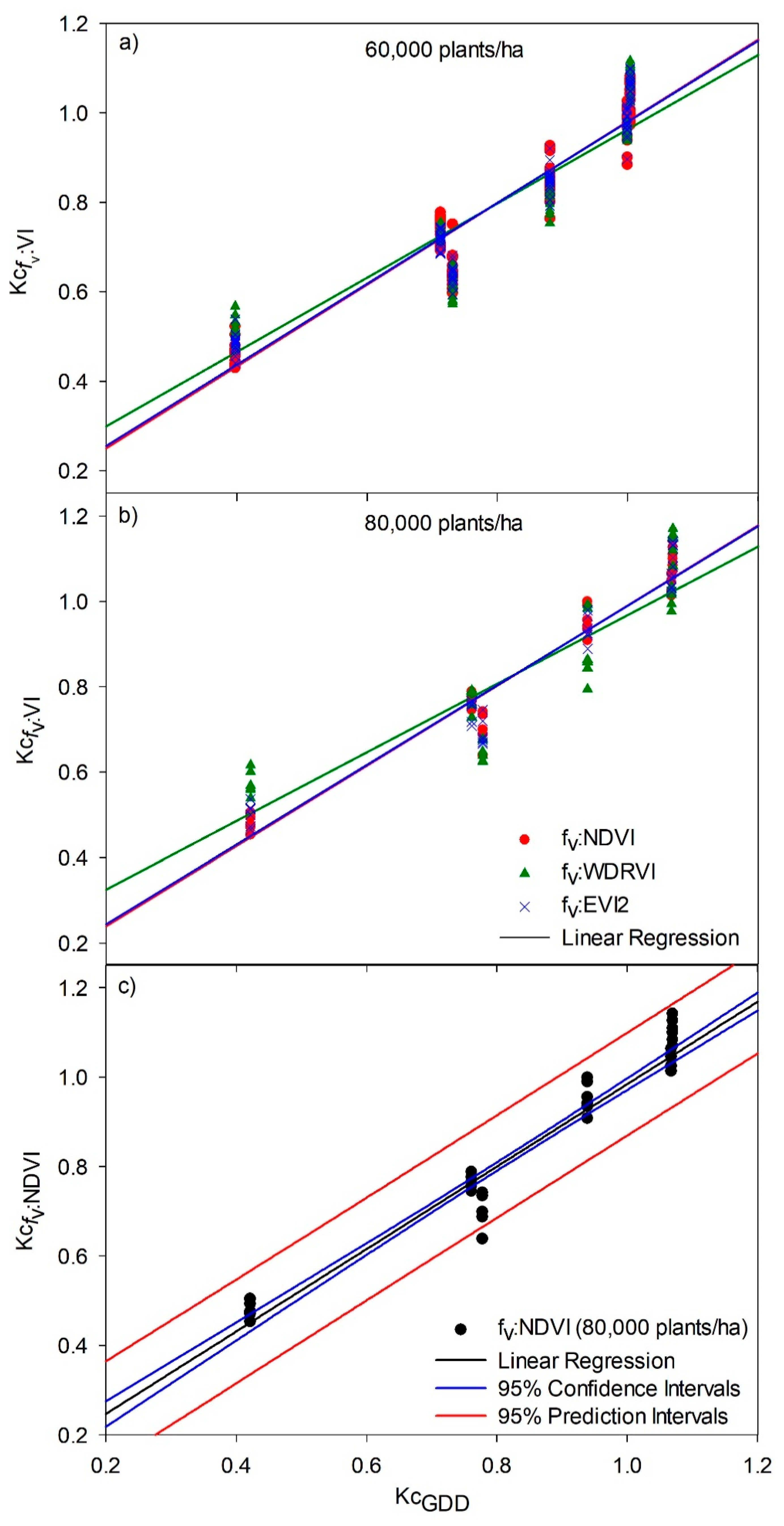
Validation of Kc_fv:VIs Models

The validation of Kc_fv:VI models is based on statistical analysis of performance indicators shown on Figure 8 and

Table 6. Performance of Kc_fv:VIs models.

Statistical Index	80,000 Plants/ha			60,000 Plants/ha
	fv:NDVI	fv:EVI2	fv:WDRVI	fv:NDVI	fv:EVI2	fv:WDRVI
CME	0.003	0.003	0.010	0.004	0.004	0.007
RMSE	0.055	0.058	0.099	0.061	0.064	0.086
MAE	0.043	0.047	0.086	0.052	0.053	0.075
E	0.960	0.955	0.871	0.929	0.923	0.860
CV (%)	6.55	6.97	11.80	7.78	8.07	10.91

, respectively. Our results reveal that the model that best estimates Kc is f_v:NDVI since it showed lower RMSE (0.055–0.061), higher efficiency (E = 92–96%), and lower CV (7.78–6.55); f_v:WRDVI and f_v:EVI2 models presented RMSE > 0.064, E < 95% and CV > 6.97.

All vegetation indices show a better performance in 80,000 plants/ha plots than 60,000 plants/ha plots. These results indicate that estimation of Kc in low-planting densities, using high spatial resolution images obtained from UAV, is good as long as f_v is high and soil evaporation is negligible, as reported by Er-Raki et al. [70] and Farg et al. [14]. Furthermore, multispectral vegetation indices (NDVI, WRDVI, and EVI2) obtained from UAV images, and Kc values calculated (Kc-c_GDD) and predicted (Kc_fv:VI) follow the same trend through the different growth stages. f_v:NDVI and f_v:EVI2 are similar in performance parameters and linear regression validation, although f_v:NDVI is slightly more accurate. These results indicate that when vegetation is isolated from the ground at a high spatial resolution, NDVI can overcome problems with high canopy density and lead to better results than EVI2 and WDRVI. Using generated models, the spatial distribution of crop Kc can be determined. Figure 9 shows, as an example, the maps of Kc for high density estimated for all pixels (case 1) and for only green pixels (case 2).

For Figure 9 calculated spectral-based values are: f_v = 0.913 and average green NDVI = 0.733, then the estimated Kc_fv:NDVI = 1.064 based on parameters indicated in Table 5 for the Kc_fv:NDVI model. The model is the most accurate model, since the Kc_fv:NDVI value is almost equal to the observed Kc_GDD = 1.069. In contrast, the average Kc values without considering f_v for cases 1 and 2 are 1.157 and 1.049, respectively.

One additional advantage of the Kc_fv:NDVI model is the it can be used to estimate areal Kc that can be applied to compute water needs in irrigation management units such as furrow, border or basin in surface irrigation, as well a tree or row-crop in micro-irrigation.

The results indicate that the use of spectral models to estimate Kc based on high spatial and temporal resolution UAV-images, using only green pixels to compute VI and f_v crop variables, offers an accurate and simple tool for ETc assessment to support irrigation scheduling in agricultural areas.

4. Conclusions

The results indicate that Kc prediction accuracy increases as Kc is expressed as a function of the VF multiplied by VI, both obtained from UAV multispectral images. Splitting and classifying pixels of vegetation, shadow, and soil, and isolating their effects were crucial to improve the model performance.

UAV-based images provided detailed spectral crop information to estimate Kc values throughout the phenological season. On the other hand, the GDD approach is a powerful Kc estimation tool to better adjust to phenology and local-scale environmental conditions. Kc values obtained from spectral data were validated with accurate GDD-based Kc values using experimental crop data with two planting densities.

This study indicates that three spectral-based Kc models showed good performance (R2 > 0.80). The model that best fit the Kc values was f_v:NDVI (R2 = 0.91 to 0.94). f_v:EVI2 and f_v:WDRVI models showed lower performance, indicating that UAV images when vegetation is isolated from soil in high spatial resolution overcome the weaknesses of the NDVI index. It can reach saturation spectral values due to high canopy density or by changes in background conditions through soil brightness or surface soil moisture content. Since the Kc_fv:NDVI model is not based in one pixel but grouped pixels in a cropped area, it can be used to estimate areal Kc which is more powerful for irrigation management purposes.

This study concludes that the use of spectral models for Kc estimation based on high spatial and temporal resolution reflectance values, once they are validated locally with experimental data, offers a powerful and simple tool for ETc estimation to support irrigation scheduling in agricultural areas.

References

1. Allen, R.G.; Pereira, L.S.; Raes, D.; Smith, M. Crop Evapotranspiration—Guidelines for Computing Crop Water Requirements—FAO Irrigation and Drainage Paper 56; FAO: Rome, Italy, 1998; ISBN 9251042195. [Google Scholar] [CrossRef]
2. Pereira, L.S.; Allen, R.G.; Smith, M.; Raes, D. Crop evapotranspiration estimation with FAO56: Past and future. Agric. Water Manag. 2015, 147, 4–20. [Google Scholar] [CrossRef]
3. Suvočarev, K.; Blanco, O.; Faci, J.M.; Medina, E.T.; Martínez-Cob, A. Transpiration of table grape (Vitis vinifera L.) trained on an overhead trellis system under netting. Irrig. Sci. 2013, 31, 1289–1302. [Google Scholar] [CrossRef] [Green Version]
4. Kamble, B.; Kilic, A.; Hubbard, K. Estimating crop coefficients using remote sensing-based vegetation index. Remote Sens. 2013, 5, 1588–1602. [Google Scholar] [CrossRef] [Green Version]
5. Singh, R.K.; Irmak, A. Estimation of crop coefficients using satellite remote sensing. J. Irrig. Drain. Eng. 2009, 135, 597–608. [Google Scholar] [CrossRef]
6. Ojeda-Bustamante, W.; Sifuentes-Ibarra, E.; Slack, D.C.; Carrillo, M. Generalization of irrigation scheduling parameters using the Growing Degree Days concept: Application to a potato crop. Irrig. Drain. 2004, 53, 251–261. [Google Scholar] [CrossRef]
7. Campos, I.; Neale, C.M.U.; Calera, A.; Balbontín, C.; González-Piqueras, J. Assessing satellite-based basal crop coefficients for irrigated grapes (Vitis vinifera L.). Agric. Water Manag. 2010, 98, 45–54. [Google Scholar] [CrossRef]
8. Rafn, E.B.; Contor, B.; Ames, D.P. Evaluation of a method for estimating irrigated crop-evapotranspiration coefficients from remotely sensed data in Idaho. J. Irrig. Drain. Eng. 2008, 34, 722–729. [Google Scholar] [CrossRef]
9. Tasumi, M.; Allen, R.G.; Trezza, R.; Wright, J.L. Satellite-based energy balance to assess within-population variance of crop coefficient curves. J. Irrig. Drain. Eng. 2005, 131, 94–109. [Google Scholar] [CrossRef]
10. Bausch, W.C. Soil background effects on reflectance-based crop coefficients for corn. Remote Sens. Environ. 1993, 46, 213–222. [Google Scholar] [CrossRef]
11. Calera, A.; Campos, I.; Osann, A.; D’Urso, G.; Menenti, M. Remote sensing for crop water management: From ET modelling to services for the end users. Sensors 2017, 17, 1104. [Google Scholar] [CrossRef] [Green Version]
12. Glenn, E.P.; Huete, A.R.; Nagler, P.L.; Nelson, S.G. Relationship between remotely-sensed vegetation indices, canopy attributes and plant physiological processes: What vegetation indices can and cannot tell us about the landscape. Sensors 2008, 8, 2136–2160. [Google Scholar] [CrossRef] [Green Version]
13. Kross, A.; McNairn, H.; Lapen, D.; Sunohara, M.; Champagne, C. Assessment of RapidEye vegetation indices for estimation of leaf area index and biomass in corn and soybean crops. Int. J. Appl. Earth Obs. Geoinf. 2015, 34, 235–248. [Google Scholar] [CrossRef] [Green Version]
14. Farg, E.; Arafat, S.M.; Abd El-Wahed, M.S.; El-Gindy, A.M. Estimation of evapotranspiration ETc and crop coefficient K c of wheat, in south nile delta of Egypt using integrated FAO-56 approach and remote sensing data. Egypt. J. Remote Sens. Space Sci. 2012, 15, 83–89. [Google Scholar] [CrossRef] [Green Version]
15. Pôças, I.; Paço, T.A.; Paredes, P.; Cunha, M.; Pereira, L.S. Estimation of actual crop coefficients using remotely sensed vegetation indices and soil water balance modelled data. Remote Sens. 2015, 7, 2373–2400. [Google Scholar] [CrossRef] [Green Version]
16. Hunsaker, D.J.; Pinter, P.J.; Kimball, B.A. Wheat basal crop coefficients determined by normalized difference vegetation index. Irrig. Sci. 2005, 24, 1–14. [Google Scholar] [CrossRef]
17. Gontia, N.K.; Tiwari, K.N. Estimation of crop coefficient and evapotranspiration of wheat (Triticum aestivum) in an irrigation command using remote sensing and GIS. Water Resour. Manag. 2010, 24, 1399–1414. [Google Scholar] [CrossRef]
18. Zhang, Y.; Han, W.; Niu, X.; Li, G. Maize crop coefficient estimated from UAV-measured multispectral vegetation indices. Sensors 2019, 19, 5250. [Google Scholar] [CrossRef] [PubMed] [Green Version]
19. Campos, I.; Neale, C.M.U.; Suyker, A.E.; Arkebauer, T.J.; Gonçalves, I.Z. Reflectance-based crop coefficients REDUX: For operational evapotranspiration estimates in the age of high producing hybrid varieties. Agric. Water Manag. 2017, 187, 140–153. [Google Scholar] [CrossRef] [Green Version]
20. Jayanthi, H.; Neale, C.M.U.; Wright, J.L. Development and validation of canopy reflectance-based crop coefficient for potato. Agric. Water Manag. 2007, 88, 235–246. [Google Scholar] [CrossRef]
21. Odi-Lara, M.; Campos, I.; Neale, C.M.U.; Ortega-Farías, S.; Poblete-Echeverría, C.; Balbontín, C.; Calera, A. Estimating evapotranspiration of an apple orchard using a remote sensing-based soil water balance. Remote Sens. 2016, 8, 253. [Google Scholar] [CrossRef] [Green Version]
22. Allen, R.G.; Pereira, L.S.; Smith, M.; Raes, D.; Wright, J.L. FAO-56 dual crop coefficient method for estimating evaporation from soil and application extensions. J. Irrig. Drain. Eng. 2005, 131, 2–13. [Google Scholar] [CrossRef] [Green Version]
23. Gitelson, A.A.; Viña, A.; Arkebauer, T.J.; Rundquist, D.C.; Keydan, G.; Leavitt, B. Remote estimation of leaf area index and green leaf biomass in maize canopies. Geophys. Res. Lett. 2003, 30, 1248. [Google Scholar] [CrossRef] [Green Version]
24. Huete, A.R.; Jackson, R.D.; Post, D.F. Spectral response of a plant canopy with different soil backgrounds. Remote Sens. Environ. 1985, 17, 37–53. [Google Scholar] [CrossRef]
25. Xiang, H.; Tian, L. An automated stand-alone in-field remote sensing system (SIRSS) for in-season crop monitoring. Comput. Electron. Agric. 2011, 78, 1–8. [Google Scholar] [CrossRef]
26. Cilia, C.; Panigada, C.; Rossini, M.; Meroni, M.; Busetto, L.; Amaducci, S.; Boschetti, M.; Picchi, V.; Colombo, R. Nitrogen status assessment for variable rate fertilization in maize through hyperspectral imagery. Remote Sens. 2014, 6, 6549–6565. [Google Scholar] [CrossRef] [Green Version]
27. Berni, J.A.J.; Zarco-Tejada, P.J.; Suárez, L.; González-Dugo, V.; Fereres, E. Remote sensing of vegetation from UAV platforms using lightweight multispectral and thermal imaging sensors. In Proceedings of the International Archives of the Photogrammetry, Remote Sensing and Spatial Information Sciences; Heipke, C., Jacobsen, K., Müller, S., Sörgel, U., Eds.; ISPRS Archives: Hannover, Germany, 2009; p. 6. [Google Scholar]
28. You, X.; Meng, J.; Zhang, M.; Dong, T. Remote sensing based detection of crop phenology for agricultural zones in China using a new threshold method. Remote Sens. 2013, 5, 3190–3211. [Google Scholar] [CrossRef] [Green Version]
29. Nguy-Robertson, A.; Gitelson, A.; Peng, Y.; Walter-Shea, E.; Leavitt, B.; Arkebauer, T. Continuous monitoring of crop reflectance, vegetation fraction, and identification of developmental stages using a four band radiometer. Agron. J. 2013, 105, 1769–1779. [Google Scholar] [CrossRef] [Green Version]
30. Marcial-Pablo, M.D.J.; Gonzalez-Sanchez, A.; Jimenez-Jimenez, S.I.; Ontiveros-Capurata, R.E.; Ojeda-Bustamante, W. Estimation of vegetation fraction using RGB and multispectral images from UAV. Int. J. Remote Sens. 2019, 40, 420–438. [Google Scholar] [CrossRef]
31. Johnson, L.F.; Trout, T.J. Satellite NDVI assisted monitoring of vegetable crop evapotranspiration in California’s San Joaquin valley. Remote Sens. 2012, 4, 439–455. [Google Scholar] [CrossRef] [Green Version]
32. Ventura, F.; Vignudelli, M.; Letterio, T.; Gentile, S.L.; Anconelli, S. Remote sensing and UAV vegetation index comparison with on-site FAPAR measurement. In Proceedings of the 2019 IEEE International Workshop on Metrology for Agriculture and Forestry, Portici, Italy, 24–26 October 2019; pp. 202–206. [Google Scholar] [CrossRef]
33. Huang, C.; Wei, H.-L.; Rau, J.-Y.; Jhan, J.-P. Use of principal components of UAV-acquired narrow-band multispectral imagery to map the diverse low stature vegetation fAPAR. GISci. Remote Sens. 2019, 56, 605–623. [Google Scholar] [CrossRef]
34. Kullberg, E.G.; DeJonge, K.C.; Chávez, J.L. Evaluation of thermal remote sensing indices to estimate crop evapotranspiration coefficients. Agric. Water Manag. 2017, 179, 64–73. [Google Scholar] [CrossRef] [Green Version]
35. Ritchie, S.; Hanway, J.; Benson, G. How a Corn Plant Develops; ISBN Special Report No. 48; Iowa State University of Science and Technology Cooperative Extension Service: Ames, IA, USA, 1986. [Google Scholar]
36. Jensen, M.; Robb, C.N.; Franzoy, E. Scheduling irrigations using climate-crop-soil data. J. Irrig. Drain. Div. 1970, 96, 25–37. [Google Scholar] [CrossRef]
37. Ojeda-Bustamante, W.; Sifuentes-Ibarra, E.; Unland-Weiss, H. Programación intergral del riego en Maíz en el Norte de Sinaloa, México. Agrociencia 2006, 40, 13–25. [Google Scholar]
38. Fareed, N.; Rehman, K. Integration of remote sensing and GIS to extract plantation rows from a drone-based image point cloud digital surface model. ISPRS Int. J. Geo-Inf. 2020, 9, 151. [Google Scholar] [CrossRef] [Green Version]
39. Peña-Barragán, J.M.; Ngugi, M.K.; Plant, R.E.; Six, J. Object-based crop identification using multiple vegetation indices, textural features and crop phenology. Remote Sens. Environ. 2011, 115, 1301–1316. [Google Scholar] [CrossRef]
40. Baatz, M.; Schape, A. Multiresolution segmentation—An optimization approach for high quality multi-scale image segmentation. In Angewandte Geographische Informations-Verarbeitung XII; Strobl, J., Blaschke, T., Griesbner, G., Eds.; Wichmann Verlag: Karlsruhe, Germany, 2000; pp. 12–23. [Google Scholar]
41. Torres-Sánchez, J.; López-Granados, F.; Serrano, N.; Arquero, O.; Peña, J.M. High-throughput 3-D monitoring of agricultural-tree plantations with Unmanned Aerial Vehicle (UAV) technology. PLoS ONE 2015, 10, e0130479. [Google Scholar] [CrossRef] [Green Version]
42. Torres-Sánchez, J.; Peña, J.M.; de Castro, A.I.; López-Granados, F. Multi-temporal mapping of the vegetation fraction in early-season wheat fields using images from UAV. Comput. Electron. Agric. 2014, 103, 104–113. [Google Scholar] [CrossRef]
43. Peña, J.M.; Torres-Sánchez, J.; de Castro, A.I.; Kelly, M.; López-Granados, F. Weed mapping in early-season maize fields using object-based analysis of Unmanned Aerial Vehicle (UAV) images. PLoS ONE 2013, 8, e77151. [Google Scholar] [CrossRef] [Green Version]
44. Drǎguţ, L.; Tiede, D.; Levick, S.R. ESP: A tool to estimate scale parameter for multiresolution image segmentation of remotely sensed data. Int. J. Geogr. Inf. Sci. 2010, 24, 859–871. [Google Scholar] [CrossRef]
45. Drǎguţ, L.; Csillik, O.; Eisank, C.; Tiede, D. Automated parameterisation for multi-scale image segmentation on multiple layers. ISPRS J. Photogramm. Remote Sens. 2014, 88, 119–127. [Google Scholar] [CrossRef] [Green Version]
46. Rouse, J.W.; Haas, R.H.; Schell, J.A.; Deering, D.W. Monitoring vegetation systems in the great plains with ERTS. In Proceedings of the Third ERTS Symposium, Washington, DC, USA, 10–14 December 1973; pp. 309–317. [Google Scholar]
47. Gitelson, A.A. Wide dynamic range vegetation index for remote quantification of biophysical characteristics of vegetation. J. Plant Physiol. 2004, 161, 165–173. [Google Scholar] [CrossRef] [PubMed] [Green Version]
48. Jiang, Z.; Huete, A.R.; Didan, K.; Miura, T. Development of a two-band enhanced vegetation index without a blue band. Remote Sens. Environ. 2008, 3833–3845. [Google Scholar] [CrossRef]
49. Wu, C.-D.; McNeely, E.; Cedeño-Laurent, J.G.; Pan, W.-C.; Adamkiewicz, G.; Dominici, F.; Lung, S.-C.C.; Su, H.-J.; Spengler, J.D. Linking student performance in massachusetts elementary schools with the “greenness” of school surroundings using remote sensing. PLoS ONE 2014, 9, e108548. [Google Scholar] [CrossRef]
50. Raj, R.; Kar, S.; Nandan, R.; Jagarlapudi, A. Precision agriculture and Unmanned Aerial Vehicles (UAVs). In Unmanned Aerial Vehicle: Applications in Agriculture and Environment; Springer International Publishing: Cham, Switzerland, 2020; pp. 7–23. [Google Scholar] [CrossRef]
51. Gitelson, A.A.; Wardlow, B.D.; Keydan, G.P.; Leavitt, B. An evaluation of MODIS 250-m data for green LAI estimation in crops. Geophys. Res. Lett. 2007, 34, L20403. [Google Scholar] [CrossRef]
52. Kim, Y.; Huete, A.R.; Miura, T.; Jiang, Z. Spectral compatibility of vegetation indices across sensors: Band decomposition analysis with Hyperion data. J. Appl. Remote Sens. 2010, 043520. [Google Scholar] [CrossRef]
53. Rocha, A.V.; Shaver, G.R. Advantages of a two band EVI calculated from solar and photosynthetically active radiation fluxes. Agric. For. Meteorol. 2009, 149, 1560–1563. [Google Scholar] [CrossRef]
54. Mondal, P. Quantifying surface gradients with a 2-band Enhanced Vegetation Index (EVI2). Ecol. Indic. 2011, 11, 918–924. [Google Scholar] [CrossRef]
55. Zhang, X. Reconstruction of a complete global time series of daily vegetation index trajectory from long-term AVHRR data. Remote Sens. Environ. 2015, 156, 457–472. [Google Scholar] [CrossRef]
56. Calera, A.; Martínez, C.; Melia, J. A procedure for obtaining green plant cover: Relation to NDVI in a case study for barley. Int. J. Remote Sens. 2001, 22, 3357–3362. [Google Scholar] [CrossRef]
57. Goward, S.N.; Huemmrich, K.F. Vegetation canopy PAR absorptance and the normalized difference vegetation index: An assessment using the SAIL model. Remote Sens. Environ. 1992, 39, 119–140. [Google Scholar] [CrossRef]
58. Deardorff, J.W. Efficient prediction of ground surface temperature and moisture, with inclusion of a layer of vegetation. J. Geophys. Res. 1978, 83, 1889–1903. [Google Scholar] [CrossRef] [Green Version]
59. Grattan, S.R.; Bowers, W.; Dong, A.; Snyder, R.L.; Carroll, J.J.; George, W. New crop coefficients estimate water use of vegetables, row crops. Calif. Agric. 1998, 52, 16–21. [Google Scholar] [CrossRef] [Green Version]
60. Willmott, C.J.; Matsuura, K. Advantages of the Mean Absolute Error (MAE) over the Root Mean Square Error (RMSE) in assessing average model performance. Clim. Res. 2005, 30, 79–82. [Google Scholar] [CrossRef]
61. Willmott, C.J. Some comments on the evaluation of model performance. Bull. Am. Meteorol. Soc. 1982, 63, 1309–1313. [Google Scholar] [CrossRef] [Green Version]
62. Zhang, L.; Sun, X.; Wu, T.; Zhang, H. An analysis of shadow effects on spectral vegetation indexes using a ground-based imaging spectrometer. IEEE Geosci. Remote Sens. Lett. 2015, 12, 2188–2192. [Google Scholar] [CrossRef]
63. Xin, J.; Yu, Z.; van Leeuwen, L.; Driessen, P.M. Mapping crop key phenological stages in the North China Plain using NOAA time series images. Int. J. Appl. Earth Obs. Geoinf. 2002, 4, 109–117. [Google Scholar] [CrossRef]
64. Calera, A.; González-Piqueras, J.; Melia, J. Monitoring barley and corn growth from remote sensing data at field scale. Int. J. Remote Sens. 2004, 25, 97–109. [Google Scholar] [CrossRef]
65. Gitelson, A.A.; Peng, Y.; Huemmrich, K.F. Relationship between fraction of radiation absorbed by photosynthesizing maize and soybean canopies and NDVI from remotely sensed data taken at close range and from MODIS 250 m resolution data. Remote Sens. Environ. 2014, 147, 108–120. [Google Scholar] [CrossRef] [Green Version]
66. Raun, W.R.; Solie, J.B.; Martin, K.L.; Freeman, K.W.; Stone, M.L.; Johnson, G.V.; Mullen, R.W. Growth stage, development, and spatial variability in corn evaluated using optical sensor readings: Contribution from the Oklahoma Agricultural Experiment Station and the International Maize and Wheat Improvement Center (CIMMYT). J. Plant Nutr. 2005, 28, 173–182. [Google Scholar] [CrossRef]
67. Guzinski, R. Comparison of Vegetation Indices to Determine Their Accuracy in Predicting Spring Phenology of Swedish Ecosystems; Lund University: Lund, Sweden, 2010. [Google Scholar]
68. Choudhury, B.J.; Ahmed, N.U.; Idso, S.B.; Reginato, R.J.; Daughtry, C.S.T. Relations between evaporation coefficients and vegetation indices studied by model simulations. Remote Sens. Environ. 1994, 50, 1–17. [Google Scholar] [CrossRef]
69. Spiliotopoulos, M.; Loukas, A. Hybrid methodology for the estimation of crop coefficients based on satellite imagery and ground-based measurements. Water 2019, 11, 1364. [Google Scholar] [CrossRef] [Green Version]
70. Er-Raki, S.; Chehbouni, A.; Guemouria, N.; Duchemin, B.; Ezzahar, J.; Hadria, R. Combining FAO-56 model and ground-based remote sensing to estimate water consumptions of wheat crops in a semi-arid region. Agric. Water Manag. 2007, 87, 41–54. [Google Scholar] [CrossRef] [Green Version]
Figure 1. Location of the study area: (a) macro-location, (b) experimental plots, (c) flight path of Unmanned Aerial Vehicles (UAV), (d) UAV acquiring aerial images, (e) plots’ maize in two growth stages.
Agronomy 11 00668 g001
Figure 2. The automated workflow implemented in Pix4D batch-processing. Adapted from [38].
Agronomy 11 00668 g002
Figure 3. Examples of orthomosaics processed at two phenological stages of the crop: 12 leaves (left) and beginning maturity (right) in three views and two density plants plots.
Agronomy 11 00668 g003
Figure 4. Resulting processed UAV-images for (a) Ortomosaic (b) OBIA segmentation, classification images with (c) three classes (vegetation, soil, shadow) and (d) only one class (vegetation).
Agronomy 11 00668 g004
Figure 5. Variation of crop coefficient (Kc)-Cumulative Growing Degree Days (CGDD) values for maize in optimal and stressed conditions.
Agronomy 11 00668 g005
Figure 6. Vegetation spectral indices (VIs)—CGDD relationship with all plots’ values, estimated based on case 2.
Agronomy 11 00668 g006
Figure 7. Linear regression between y = KcGDD and x = fv*VIs for two planting densities for the three VIs: (a) Normalized Difference Vegetation Index (NDVI), (b) EVI2 and (c) WDRVI. It is also shown in (c) the phenological stage with an ID digit according to Table 4.
Agronomy 11 00668 g007
Figure 8. Validation of the Kcfv:VIs models as a function of KcGDD for two plant densities (a) 60,000 plants/ha and (b) 80,000 plants/ha. and (c) 95% Confidence and prediction intervals for Kcfv:NDVI values for 80,000 plants/ha.
Agronomy 11 00668 g008
Figure 9. Spatial distribution of Kc values estimated for cases 1 and 2, from UAV images for the high-density planting plot at CGDD = 1033.
Agronomy 11 00668 g009