Article

Exploring Climate Change Effects on Vegetation Phenology by MOD13Q1 Data: The Piemonte Region Case Study in the Period 2001–2019

by
Filippo Sarvia
,
Samuele De Petris
and
Enrico Borgogno-Mondino
*
Department of Agricultural, Forest and Food Sciences, University of Turin, L.go Braccini 2, 10095 Grugliasco, Italy
*
Author to whom correspondence should be addressed.
Agronomy 2021, 11(3), 555; https://doi.org/10.3390/agronomy11030555
Submission received: 10 February 2021 / Revised: 5 March 2021 / Accepted: 9 March 2021 / Published: 15 March 2021
(This article belongs to the Special Issue Remote Sensing in Agriculture)

Abstract

:
Rising temperature, rainfall, and wind regime changes, increasing of frequency and intensity of extreme events are only some of the effects of climate change affecting the agro-forestry sector. Earth Observation data from satellite missions (often available for free) can certainly support analysis of climate change effects on vegetation, making possible to improve land management in space and time. Within this context, the present work aims at investigating natural and agricultural vegetation, as mapped by Corine Land Cover (CLC) dataset, focusing on phenological metrics trends that can be possibly conditioned by the ongoing climate-change. The study area consists of the entire Piemonte region (NW-Italy). MOD13Q1-v6 dataset from TERRA MODIS mission was used to describe pluri-annual (2001–2019) phenological behavior of vegetation focusing on the following CLC classes: Non-irrigated arable land, Vineyards, Pastures, and Forests. After computing and mapping some phenological metrics as derivable from the interpretation of at-pixel level NDVI (Normalized Difference Vegetation Index) temporal profile, we found that the most significant one was the maximum annual NDVI (MaxNDVI). Consequently, its trend was analyzed at CLC class level for the whole Piemonte region. Natural and semi-natural vegetation classes (Pastures and Forests) were furtherly investigated testing significance of the Percent Total Variation (TV%) of MaxNDVI in the period 2001–2019 for different altitude classes. Results proved that Non-irrigated arable land showed a not significant trend of MaxNDVI; differently, vineyards and forests showed a significant increasing one. Concerning TV%, it was found that it increases with altitude for the Forests CLC class, while it decreases with altitude for the pastures class.

1. Introduction

Humans have always interacted with environment; through their activities, they have modified and adapted natural environment by continuing to take advantage of resources over time. Starting from the second half of the 18th century, man has prevailed over environment and, during the last century, ecosystems structure has been changing much more rapidly than in the past [1]. According to the Global Environment Outlook [2], the planet is suffering the sixth great extinction that for the first time will be not due to natural global changes, but rather to human activity [3].
Rising temperatures, changes in rainfall and wind regime, and changes in frequency and intensity of extreme events are the main factors conditioning animal and plant species [4]. These events regulate environmental characteristics like the availability of nutrients, essential for the development of primary producers, ice cover and, in the sea, the intensity of convective movements, transparency, and water level. With these premises, it is mandatory to consider response times characterizing those processes influenced by climate change: from the short times for impacts on physiology (day–months) to the longer ones for area changes (year–decades), up to the typical scales of evolutionary processes (hundreds of year–millennia) [5,6].
Plants are very sensitive to climate and its variations: distribution of vegetative types defines the bioclimatic zones (or belts), whereas phenology is strictly dependent on seasonal meteorological trend [7,8]. Consequently, climate change could lead to changes in geographical distribution of species and, contemporarily, to timely shift appearance of plant pheno-phases, with probable consequences on crop productivity and landscape in general [9,10]. In particular, vegetation trend changes could be related to vegetation management, climate and climate change as deeply discussed in literature [11,12,13]. Phenological observations and agronomic calendars have been used by humans for thousands of years and long historical time series of such information can be found in many documents. There are, in fact, important historical archives: some records from Japan date back to the early 1800s [14]; some from Europe go back to the early 1700s [15]. More recently, over the last fifteen years, phenology has regained a new interest in the scientific community (included the European Topic Centre on Air and Climate Change (ETC-ACC) of the European Environment Agency (EEA)). Applications focusing on seasonal dynamics of vegetation [16,17,18] and phenological modelling use these data to predict capacity and productivity in agriculture [19] or as a source of robust proxies for medium and long-term effects of climatic variations.
At medium and high latitudes spring phenological phases—sprouting, foliar unfolding, and flowering—are mainly regulated by temperature, and a considerable number of studies have found good correlations between spring phenophases and air temperature [20,21,22,23,24,25]. Differently, meteo-climatic influence on autumn phenology is still unclear [26].
Satellite data and predictive model simulations are the basis to understand the climate system [27]. Satellite remote sensing for Earth Observation can effectively support this process, making possible to get information about the earth’s surface, subsoil, and atmosphere [28]. Since the first spatial observation of solar radiation and cloud reflection, remote sensing has gradually become a major research method in climate change studies [29]. The use of satellites permits the observation of states and processes of the atmosphere, earth, and oceans at different space-time scales. For example, it is one of the most efficient approaches for monitoring land cover and its changes over time at a variety of spatial scales [30,31]. Satellite data are often used in combination with climate models to simulate climate system dynamics and to improve climate forecasting [32]. The Global Climate Observing System (GCOS) has reported 26 of the 50 key climate variables (ECVs) as significantly dependent on satellite observations [33]. Remote sensing data are also largely used to develop prevention, mitigation, and adaptation measures to cope with the impact of climate change [34], to take out insurance policies based on vegetation trends [35,36,37,38], to support Common Agricultural Policy control in agriculture [39], to support wildlife diseases assessment [40], to manage the risk of falling trees and heat islands monitoring [41,42,43]. Studies on climate change, in fact, need continuous calibration and validation data and appropriate temporal and spatial sampling over a long period of time [44].

Study Aims

The aims of this work were to assess how low spatial resolution satellite data from TERRA MODIS mission can evaluate the effects of mid-term climate change on vegetated areas (that have not changed over time), with special concerns about annual phenological metrics as derivable from Normalized Difference Vegetation Index (NDVI) maps time series between 2001 and 2019 in the Piemonte Region.
A preliminary trend analysis was performed to test the presence of climate change in area of interest (AOI) according to regional meteorological stations. Consequently vegetated “natural/semi natural” (forests and pastures) and “managed” (agricultural) classes, derived by the Corine Land Cover (CLC), were, separately, considered. Moreover altitude effects on phenology changes were also taken into account to deepen investigation for forest and pasture classes.

2. Materials and Methods
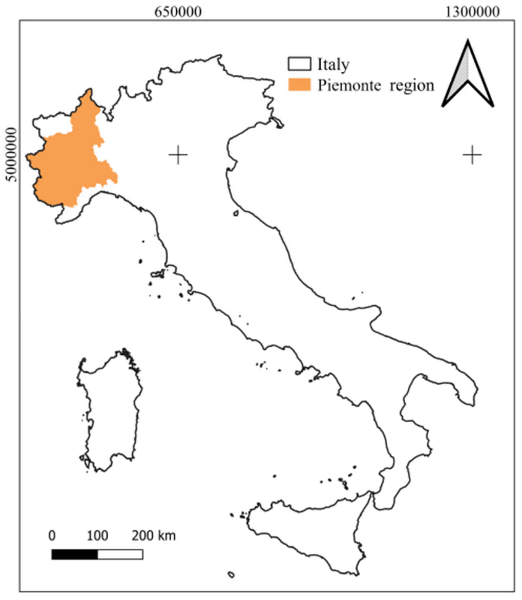
2.1. Study Area

The study area corresponds to the entire Piemonte region (North-West Italy) (Figure 1). It sizes about 25,400 km2. From a climatic point of view, North-Western Alps cause a gradual reduction of temperature while altitude increases making the local climate a typical temperate one with continental character. Average annual precipitation and temperature are 1050 mm and 11.9 °C, respectively. Thermal inversion phenomena, caused by cold air, can often affect the area, especially in the valleys.

2.2. Available Data

The following data were used: (a) MOD13Q1-v6 product from the NASA TERRA MODIS sensor; (b) 2000, 2006, 2012 and 2018 CLC datasets; (c) Digital Terrain Model (DTM) of the Piemonte Region (2011).

2.2.1. Satellite Data

Monitoring of biomass along time requires that uniform and comparable metrics are used. Vegetation Indices (VIs) from multispectral data are often used to describe vegetation cover/status and, consequently, to assess phenology with high temporal resolution [45,46]. For this reason, data form the Moderate-Resolution Imaging Spectroradiometer (MODIS) sensor, operating on TERRA satellite mission since 2000 and having 1-day temporal resolution, was taken into account. The MOD13Q1-v6 NDVI collection product, obtained from NASA’s Land Processes Distributed Active Archive Center (LPDAAC) [47], was specifically used. Data were downloaded from AppEEARS, provided as Tagged image File (TIF) georeferenced in the WGS84 geographic reference system. MOD13Q1-v6 product is a 16 days timely-spaced one, having a spatial resolution of 250 m. It is a composite product containing the “best” available local observations (at pixel level) within a 16 days period. Selection of the best pixel relies on criteria that minimize cloud cover effect and viewing angles and maximize NDVI local value (maximum in the reference period). MOD13Q1-V6 product contains many layers, included the NDVI and the pixel reliability (PR) ones. PR codes are reported in Table 1.
For this work, 437 images (MOD13Q1-v6) were obtained covering a sensing period between 1 January 2001 and 19 December 2019. Available NDVI layers allowed to generate a NDVI Time Series (NTS).

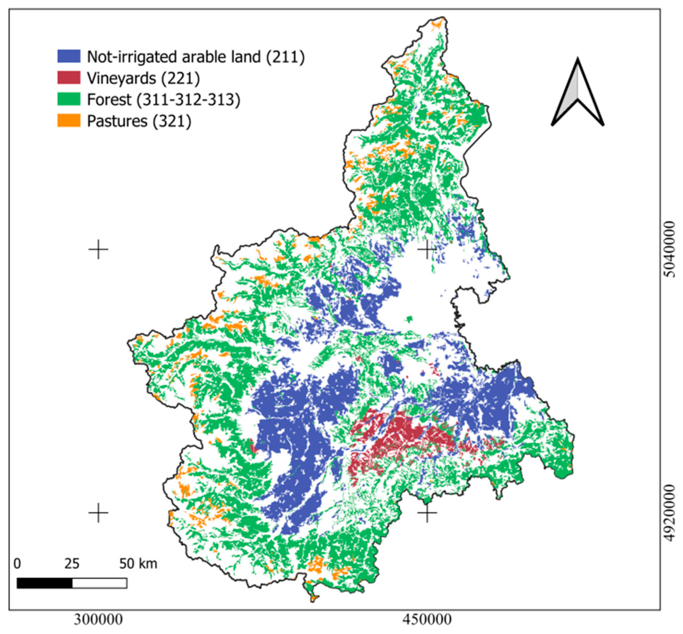
2.2.2. Land Cover Map

CORINE Land Cover—Level 3 datasets were used to map and label vegetated areas of Piemonte. CORINE datasets were obtained, for free, from the Copernicus Land Monitoring Service for the years 2000 (hereinafter CLC2000), 2006 (hereinafter CLC2006), 2012 (hereinafter CLC2012) and 2018 (hereinafter CLC2018). CLC technical features are reported in Table 2. CLC Level 3 is the most detailed one, where each patch presents more than 75% of the characteristics of a given class according to the CLC nomenclature rules [48].
All the available CLC maps were combined by intersection to recognize those patches whose meaning (class) remained the same along the entire explored period (2001–2019). Only agricultural and natural classes were considered (Table 3). Among these classes, only the Forests one includes sub-classes: deciduous forests (311), coniferous forests (312), and mixed deciduous and coniferous forests (313). Consequently, they were preventively merged into a single class (Forests) in order to define a single land cover class representative of natural vegetation conditions (no human activity is generally performed to manage tree growth). All data were finally projected into the WGS84/UTM 32N reference frame. Data processing was achieved by QGIS 3.2.0 and SAGA GIS 7.0. Statistical analysis was performed using Past 4.01.

2.2.3. Digital Terrain Model

A 25 m grid sized raster DTM (Digital Terrain Model) was obtained for free from the geoportal of the Piemonte Region administration [49]. It covers the entire regional territory and was generated from LiDAR (Light Detection and Ranging) point clouds. Native DTM, having a grid size of 5 m and a height accuracy of 0.66 m, was generalized down to a 25 m grid product, and made available for large size areas investigation. In this work, DTM was used to investigate dependence of natural and semi-natural vegetation (Pastures and Forests classes) from altitude; 4 altitudinal zones (hereinafter called AZs) were defined (Table 4) according to Mayr-Pavari bioclimatic zones [50].

2.2.4. Reference Temperature Data

In order to test climate induced trends, some ground-retrieved temperature data were used as reference. A total of 24 meteorological stations (MS) were selected from the Regional meteorological network (www.arpa.piemonte.it, accessed on: 16 January 2021) in order to explore the temperature trends in AOI. In particular daily average temperature was analyzed in the period 2000–2019 defining time series with a time step of 1 day (7671 observations for each MS). The MS selection was achieved by spatial intersection between the CLC and AZs classes previously defined. Specifically 3 MS temperature time series were collected for each CLC and AZs classes (Figure 2).

2.3. Data Processing

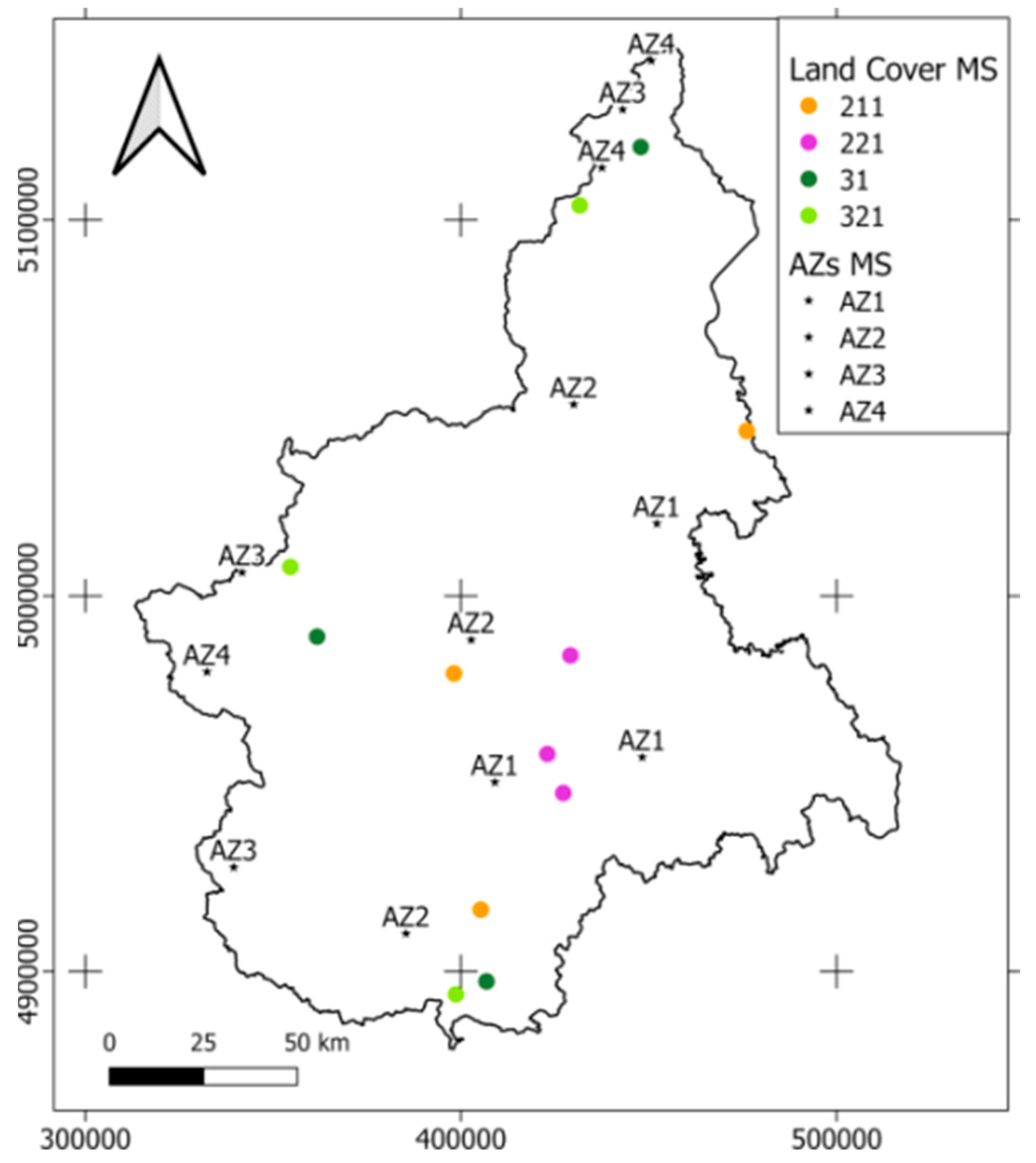
2.3.1. Reference Classes and Patches Selection

Selection of unchanged CLC patches, i.e., maintaining the same class meaning along time, is mandatory while investigating climate trends along time (2001–2019) at class level. This step is basic to avoid misleading deductions that could significantly compromise time trend analysis. For example, NDVI trend of a forest area will certainly change if, in the meantime, it turns to urban. For this reason, a preliminary step was performed to select only those patches (belonging to the above-mentioned classes) whose meaning remained the same in all the available 4 CLC maps. Selection was achieved by polygons intersection by ordinary GIS procedures. Results are reported in Figure 3.
Since natural and semi-natural vegetation is assumed to be more susceptible by climate change [51] in respect of agricultural vegetation, a further level of investigation was carried out for natural classes solely (Forests and Pastures).
For these two classes authors investigated the role of altitude (at AZs level) on time trends of the explored phenological metrics. CLC patches were consequently completed with the correspondent height information derived from DTM by GIS zonal statistics. Forest and Pasture classes were finally analyzed at AZs level determining a total of eight new sub-classes to analyze.
Two analyses were consequently carried out: one testing phenological metrics trend at class level with reference to classes of Table 3; one testing differences between phenological metrics trends of the same class placed at different AZ. For this second analysis Forest and Pasture classes, solely, (natural/semi-natural) were considered.

2.3.2. Temperature Trends Analysis

Starting from the MS data, the average time series was computed for each CLC and AZs classes. Resulting daily average temperature time series were analyzed by first order polynomial regression. In particular the gain values and their significance level were obtained in order to test the presence and quantify the strength of climate induced trends.
The basic assumption was that vegetation phenology is strongly affected by temperature [52,53]. Therefore an increase of temperature trend changes phenological response [54,55]. Nevertheless, human management can mitigate the climate change effects on vegetation [56].

2.3.3. Phenological Metrics (PM)

For each investigated class, the correspondent average NDVI temporal profile was computed from NTS (hereinafter called ANTS). Phenological response is strictly related to many factors as vegetation species, terrain aspect, local nutrients availability, and climate. Only the latter can be assumed homogenous over AOI while other factors are characterized by high variability necessarily affecting phenological metrics estimates. Averaging phenological profiles within the same land cover class mitigates this variability enhancing climate related effects [57,58].
A Savitzky–Golay [59] filtering was run (3rd degree local polynomial; span values = 0.016) to smooth ANTS and minimize outliers’ oscillations.
The following phenological parameters were computed at year level with the aim of summarizing annual growing season (from leaf development to leaf senescence) of vegetated classes: SOS (Start Of Season), EOS (End Of Season), LOS (Length Of Season), MaxNDVI (annual maximum NDVI value), and DOY (Day Of the Year when MaxNDVI occurs). In particular SOS is define as the moment of the year having a consistent upward trend in leaf development. Otherwise the EOS is the moment of the year having a consistent downward trend in leaf senescence. While MaxNDVI is related to maximum biomass development and maximum level of canopy photosynthetic activity [60].
SOS and EOS were calculated by a first derivative approach where SOS and EOS are located at the maximum and minimum of the 1st derivative, respectively. These moments occur where ANTS is positively and negatively steeper [61,62]. LOS was obtained by differencing of EOS and SOS; it measures the vegetative season length in the considered year.
The previously mentioned metrics describe specific moments (in the time-domain) when vegetation expresses a peculiar event (e.g., leaf development or leaf senescence), but are not able to measure the strength of canopy vigor. Many authors reported that yearly maximum NDVI value is a good metric to compare vegetation behavior throughout the years [63,64]. Consequently, yearly MaxNDVI was calculated and the corresponding DOY recorded.

2.3.4. Class Effects on PM Trends

A feasibility analysis was conducted considering the 4 CLC classes of Table 3 to determine if and how phenological metrics showed significant trends, in the reference period, possibly relatable to climate change. All the above mentioned phenological metrics were consequently compared along the explored 19 years and fitted by a first order polynomial regressive model (ordinary least squares). Gain values of the calibrated model and the correspondent significance level (α = 0.05) were assessed to test if any of the considered PM showed climate-induced significant variations [65].

2.3.5. Altitudinal Effects on PM Trends

A further assessment was done to refine deductions about natural (Forests) and semi-natural (Pastures) vegetation. These 2 classes were split in 4 sub-classes each, according to the 4 defined AZs. Investigation concerned only the MaxNDVI metric, that the previous step indicated as the most significant one from the time trend point of view. Again, a first order polynomial linear regression was used to test strength and significance of trends. The approach is coherent with other similar works where NDVI-based vegetation changes and their responses to climate change over mountain system exploring different time range [29,66,67].
The adopted approach is the common slope test that is based on gain significance analysis [68,69] testing the hypothesis that two gain values are statistically different. It is worth to remind that gain value only defines the rate of increase/decrease of metric trends; therefore, to quantify the total variation that the considered PM suffered from in the reference period (2001–2019), the Percent Total Variation of MaxNDVI (TV%) was calculated according to Equation (1).
T V % = G · t 19 t 1 G · t 1 + O · 100
where G is the gain value of MaxNDVI linear regression model, O is the offset value and t1 and t19 are the first and the last observation respectively (2001, 2019). A final comparison to test dependency of TV% from AZs was performed by scatter plot analysis.

3. Results and Discussions

3.1. Reference Classes and Patches Selection

To map unchanged CLC classes during the period 2001–2019 a polygon layer intersection step was achieved with reference to the four CLC available maps. Statistics concerning focus classes (Non-irrigated arable land, Vineyards, Forests, and Pastures) are shown in Table 5.
It can be noted that size of all the considered CLC classes showed a decreasing trend over time. In particular, pastures decreased of 1521 km2 between 2006 and 2012, correspondent to about 70% of its value. Similar results were found by Rusu et al. in Romania for natural/semi natural areas related to deforestation and urbanization processes [70]. Future investigations could be relevant to discover the nature of this significant change in this particular area. Conversely, other classes remained almost unchanged along the entire period as also observed in other works [70]. As previously mentioned, forest and pasture classes were further divided into four sub-classes depending on AZs, whose dimension is reported in Table 6.
Table 6 shows that forests cover prevail at lower altitudes and decreases while altitude increases. More than 88% of forests class is, in fact, located between 0 and 1200 m a.s.l. Pasture class, differently, prevails at the higher altitudes (AZ4 > 2000 m a.s.l.).

3.2. Temperature Trend Assessment

Table 7 shows gain values of linear regression trends according to CLC and AZs classes.
All trends were significantly increased during the 2000–2019 period, suggesting the presence of climate change within AOI. Similar increasing trends were reported in literature [71,72], suggesting a key role of temperature in phenological development. Therefore authors used PM to assess the effects of such temperature increase (see Section 3.3).

3.3. Phenological Trend Assessment

3.3.1. Class Effects on PM Trends

Table 8 shows gain values computed for all PM and CLC classes. In particular, not for all classes, the most significant PM was MaxNDVI. This metric seems to be more sensitive to vegetation changes along time series as proved by some works [61,73] that, similarly, adopted low geometrical resolution satellite imagery. Other PMs did not show significant trends for any CLC class. The same finding was also reported in literature [56,74,75,76], in particular Tao [74] founds that MaxNDVI had a positive trend in croplands, forests and grasslands, more significant than LOS. This phenomenon could be related to two main factors: one related to the adopted product (MOD13Q1); one related to the PM itself. As far as the first one is concerned, it is worth to remind that MOD13Q1 product is a collection made of composited images, where pixel values refer to different dates, within a 16 days period. This, considerably, determines a significant uncertainty in SOS, EOS, and LOS estimation. As far as the second factor is concerned, PMs other than MaxNDVI are estimated looking for a single specific event along the analyzed NTS (e.g., the day of the end of season). Frequent harvests (or mowing) of crops, ordinarily performed in an agriculture context, certainly affect EOS/LOS estimates, especially when moderate resolution images are used, making them particularly uncertain. Among tested trends, only those related to Forests (natural) and Vineyards (agricultural with no water management) resulted significant. This suggests that human practices can mitigate effects of climate changes over vegetation; in fact, irrigated and fertilized agricultural classes did not show significant trend. Pastures is ordinarily considered a semi-natural system, but, unexpectedly, they did not show any significant trend; this is possibly due to their intensive management that is performed in Piemonte, especially in lowland areas. Similar results were obtained by Tang et al. [56] and Menzel et al. [56,71], specifically both studies showed that the effects of climate change on vegetation identified by PM changed in relation to the land cover. In particular, they noted that the agricultural class was poorly affected by climate change, while the forest one was the most susceptible to the climate effects.

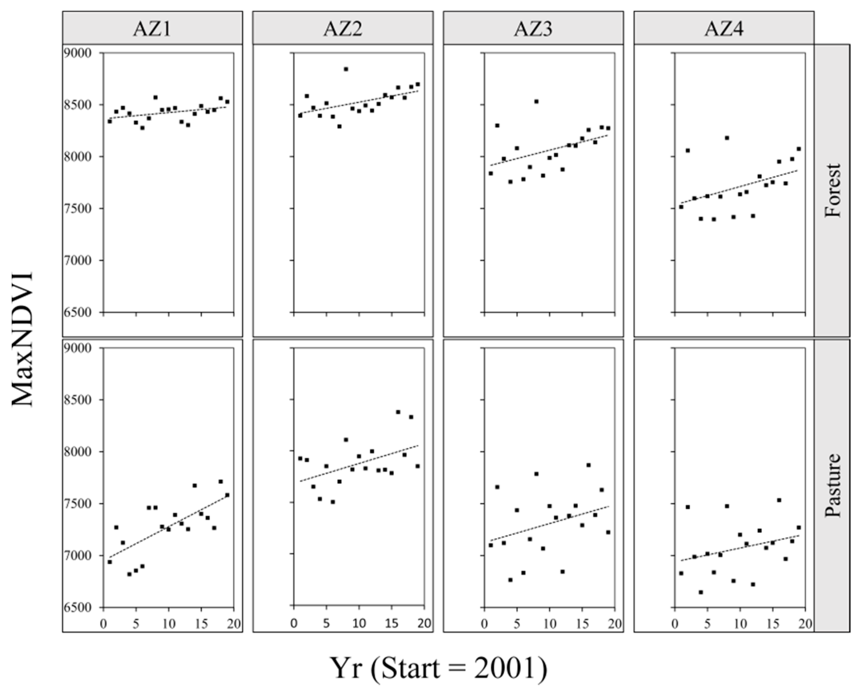
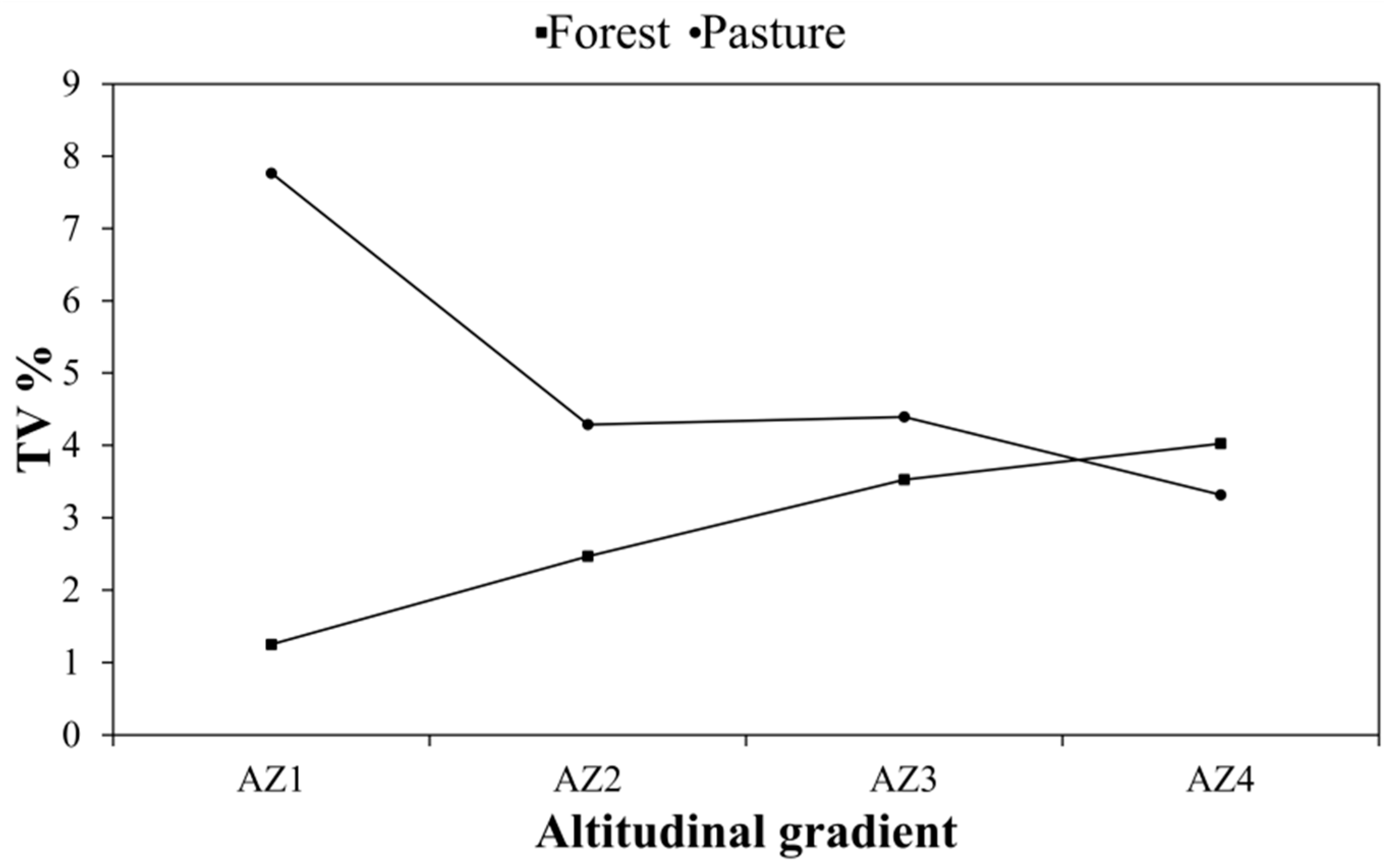
3.3.2. Altitudinal Effects on PM Trends

MaxNDVI resulted the only PM showing a detectable and significant trend along time at the MOD13Q1 temporal and spatial scale. Consequently, a further analysis was performed to explore the dependence of its trends from altitude. Only natural and semi-natural vegetation were considered at this point. Similarly, as previously done, first order polynomial trends were tested with reference to the eight classes of Table 6. Results are reported in Table 9 and Figure 4.
Table 10 reports p-values resulting from the common gain test performed for all the AZs of forest and pasture classes. In general, results indicate that no significant differences exist between gains of AZs trends for both forests and pastures. Nevertheless, according to Table 9, such trends show a positive value. These results suggest that climate change effects on MaxNDVI, i.e., vegetation vigor, is constant and latent in all the altitudinal classes. Nevertheless, this latent climatic-induced trend could vary in terms of relative strength if the vigor total variation (TV%, Equation (1)) is computed and compared with the initial MaxNDVI value.
TV% is reported against AZs in Figure 5 for both forests and pastures. Forests showed an increasing TV% gradient with AZs. Specifically, lower TV% (about 1%) correspond to forests placed at lower altitudes, suggesting that climate change determine stronger effects on forests located at higher altitudes (about 4%). Results seem to be consistent with a recent studies [74,77,78,79] that found that vegetation greening and climate warming effects trends were stronger at higher altitudes, thus supporting the idea that an altitudinal gradient effect operates in determining forests vigor level and changes.
Conversely, pastures showed a negative altitudinal TV% gradient. Pastures located at lower altitudes were more affected by climate changes than high altitude pastures. This probably relies on the fact that pastures, in lowlands, are commonly more intensively managed (irrigations and fertilizations) than in mountain. In this, human management could increase vigor and productivity of low altitude grass systems while grass systems in alpine zone (i.e., high AZs) are generally characterized by low biomass and often alternate with bare soil [80,81]; this factor certainly affects ANTS determining a minor sensitivity of phenology to climate changes. The same phenomenon was reported in Li [82] where a significant NDVI increase was primarily associated with forests, while a weak NDVI increase was observed for pastures at altitudes > 2000 m. Results are also in agreement with [83] findings that proved that main vegetation climate-related changes occur at lower altitudes for alpine pastures.

4. Conclusions

In this work, the increasing trend of temperature probably related to climate change in AOI was proved analyzing regional meteorological stations data. Therefore effects on vegetation phenology was expected. To prove such phenomenon a trend analysis of climate change effects on Piemonte Region vegetation was performed using MOD13Q1 imagery in the period 2001–2019. In particular, agricultural and natural land cover classes (as reported by CLC maps) were explored by analyzing correspondent ANTS. Some PMs were computed with reference to the yearly class ANTS, but only MaxNDVI showed significant trends possibly related to climate change for some classes at regional level. In particular, agriculture classes did not show any significant MaxNDVI trend (G = 11.285, p > 0.05); differently, forests and vineyards presented a significant positive trend (G = 10.500, p < 0.05 and G = 34.333, p < 0.01 respectively). A further analysis was conducted to assess if altitude could condition trends of natural and semi-natural classes. The common gain test proved that no significant difference exists between trends of forests classes placed at different altitudes. Similarly, for pastures. Nevertheless, while relating the absolute difference of MaxNDVI totally occurred along the entire period (2001–2019) with its initial value at 2001 (by TV%), it was observed that high altitude forests presented a higher value of TV% (4%) than low altitude ones (1%). Conversely, pastures showed higher TV% at lower (7.7%) than at higher altitudes (3.3%). In conclusion, MOD13Q1 data proved to be an effective product to monitor vegetation over time and to derived some PMs. Unfortunately, not all of them, at the temporal and spatial scale of MOD13Q1 and at the regional level of class aggregation proved to be sensitive to the ongoing climate change. Only MaxNDVI showed significant trends, at regional level, for forests and vineyards making evident that, absolutely speaking, it operated similarly at different altitude zones within the same class. Nevertheless, we showed that same absolute difference in MaxNDVI meant a different effect (measured by TV%) at different altitudes, depending on its initial value.

Author Contributions

Conceptualization, F.S. and S.D.P.; methodology, F.S., S.D.P., and E.B.-M.; software, S.D.P.; validation, F.S., and S.D.P.; formal analysis, F.S.; investigation, F.S. and S.D.P.; resources, F.S.; data curation, F.S. and S.D.P.; writing—original draft preparation, F.S., and S.D.P.; writing—review and editing, F.S., S.D.P., and E.B.-M.; visualization, F.S.; supervision, E.B.-M.; project administration, E.B.-M. All authors have read and agreed to the published version of the manuscript.

Funding

This research received no external funding.

Institutional Review Board Statement

Not applicable.

Informed Consent Statement

Informed consent was obtained from all subjects involved in the study.

Data Availability Statement

Data sharing not applicable.

Conflicts of Interest

The authors declare no conflict of interest.

References

  1. Reid, W.V.; Mooney, H.A.; Cropper, A.; Capistrano, D.; Carpenter, S.R.; Chopra, K.; Dasgupta, P.; Dietz, T.; Duraiappah, A.K.; Hassan, R.; et al. Ecosystems and Human Well-Being: Synthesis; Island Press: Washington, DC, USA, 2005. [Google Scholar]
  2. Agard, J.; Alcamo, J.; Ash, N.; Arthurton, R.; Barker, S.; Barr, J. Global Environment Outlook: Environment for Development (GEO-4); United Nations Environment Programme (UNEP): Nairobi, Kenya, 2007. [Google Scholar]
  3. Crutzen, P.J. Human Impact on Climate Has Made This the “Anthropocene Age”. New Perspect. Q. 2005, 22, 14–16. [Google Scholar] [CrossRef]
  4. White, P.S. Natural Disturbance and Patch Dynamics: An Introduction. Nat. Disturb. Patch Dyn. 1985, 3–13. [Google Scholar] [CrossRef]
  5. Parmesan, C.; Yohe, G. A Globally Coherent Fingerprint of Climate Change Impacts across Natural Systems. Nature 2003, 421, 37–42. [Google Scholar] [CrossRef]
  6. Becklin, K.M.; Anderson, J.T.; Gerhart, L.M.; Wadgymar, S.M.; Wessinger, C.A.; Ward, J.K. Examining Plant Physiological Responses to Climate Change through an Evolutionary Lens. Plant Physiol. 2016, 172, 635–649. [Google Scholar] [CrossRef] [PubMed]
  7. Parmesan, C.; Hanley, M.E. Plants and Climate Change: Complexities and Surprises. Ann. Bot. 2015, 116, 849–864. [Google Scholar] [CrossRef] [PubMed]
  8. Hawkins, B.; Sharrock, S.; Havens, K. Plants and Climate Change: Which Future? Botanic Gardens Conservation International: Richmond, UK, 2008. [Google Scholar]
  9. Pearson, R.G.; Phillips, S.J.; Loranty, M.M.; Beck, P.S.; Damoulas, T.; Knight, S.J.; Goetz, S.J. Shifts in Arctic Vegetation and Associated Feedbacks under Climate Change. Nat. Clim. Chang. 2013, 3, 673–677. [Google Scholar] [CrossRef]
  10. Blois, J.L.; Williams, J.W.; Fitzpatrick, M.C.; Ferrier, S.; Veloz, S.D.; He, F.; Liu, Z.; Manion, G.; Otto-Bliesner, B. Modeling the Climatic Drivers of Spatial Patterns in Vegetation Composition since the Last Glacial Maximum. Ecography 2013, 36, 460–473. [Google Scholar] [CrossRef]
  11. Chen, S.; Gong, B. Response and Adaptation of Agriculture to Climate Change: Evidence from China. J. Dev. Econ. 2021, 148, 102557. [Google Scholar] [CrossRef]
  12. Anwar, M.R.; Li Liu, D.; Macadam, I.; Kelly, G. Adapting Agriculture to Climate Change: A Review. Theor. Appl. Climatol. 2013, 113, 225–245. [Google Scholar] [CrossRef]
  13. Howden, S.M.; Soussana, J.-F.; Tubiello, F.N.; Chhetri, N.; Dunlop, M.; Meinke, H. Adapting Agriculture to Climate Change. Proc. Natl. Acad. Sci. USA 2007, 104, 19691–19696. [Google Scholar] [CrossRef] [Green Version]
  14. Lauscher, F. Neue Analysen Ältester Und Neuerer Phänologischer Reihen. Arch. Meteorol. Geophys. Bioklimatol. Ser. B 1978, 26, 373–385. [Google Scholar] [CrossRef]
  15. Sparks, T.H.; Carey, P.D. The Responses of Species to Climate over Two Centuries: An Analysis of the Marsham Phenological Record, 1736–1947. J. Ecol. 1995, 83, 321–329. [Google Scholar] [CrossRef]
  16. Myneni, R.B.; Keeling, C.D.; Tucker, C.J.; Asrar, G.; Nemani, R.R. Increased Plant Growth in the Northern High Latitudes from 1981 to 1991. Nature 1997, 386, 698–702. [Google Scholar] [CrossRef]
  17. Chen, Z.-J.; Li, J.-B.; Fang, K.-Y.; Davi, N.K.; He, X.-Y.; Cui, M.-X.; Zhang, X.-L.; Peng, J.-J. Seasonal Dynamics of Vegetation over the Past 100 Years Inferred from Tree Rings and Climate in Hulunbei’er Steppe, Northern China. J. Arid Environ. 2012, 83, 86–93. [Google Scholar] [CrossRef] [Green Version]
  18. Richardson, A.D.; Keenan, T.F.; Migliavacca, M.; Ryu, Y.; Sonnentag, O.; Toomey, M. Climate Change, Phenology, and Phenological Control of Vegetation Feedbacks to the Climate System. Agric. For. Meteorol. 2013, 169, 156–173. [Google Scholar] [CrossRef]
  19. Beaubien, E.G.; Freeland, H.J. Spring Phenology Trends in Alberta, Canada: Links to Ocean Temperature. Int. J. Biometeorol. 2000, 44, 53–59. [Google Scholar] [CrossRef] [PubMed]
  20. Menzel, A.; Fabian, P. Growing Season Extended in Europe. Nature 1999, 397, 659. [Google Scholar] [CrossRef]
  21. Wielgolaski, F.-E. Starting Dates and Basic Temperatures in Phenological Observations of Plants. Int. J. Biometeorol. 1999, 42, 158–168. [Google Scholar] [CrossRef]
  22. Abu-Asab, M.S.; Peterson, P.M.; Shetler, S.G.; Orli, S.S. Earlier Plant Flowering in Spring as a Response to Global Warming in the Washington, DC, Area. Biodivers. Conserv. 2001, 10, 597–612. [Google Scholar] [CrossRef]
  23. Chmielewski, F.-M.; Rötzer, T. Phenological Trends in Europe in Relation to Climatic Changes. Agrometeorol. Schr. 2000, 7, 1–15. [Google Scholar]
  24. Chmielewski, F.-M.; Müller, A.; Bruns, E. Climate Changes and Trends in Phenology of Fruit Trees and Field Crops in Germany, 1961–2000. Agric. For. Meteorol. 2004, 121, 69–78. [Google Scholar] [CrossRef]
  25. Sparks, T.H.; Menzel, A. Observed Changes in Seasons: An Overview. Int. J. Climatol. J. R. Meteorol. Soc. 2002, 22, 1715–1725. [Google Scholar] [CrossRef]
  26. Walther, G.-R.; Post, E.; Convey, P.; Menzel, A.; Parmesan, C.; Beebee, T.J.; Fromentin, J.-M.; Hoegh-Guldberg, O.; Bairlein, F. Ecological Responses to Recent Climate Change. Nature 2002, 416, 389–395. [Google Scholar] [CrossRef] [PubMed]
  27. Overpeck, J.T.; Meehl, G.A.; Bony, S.; Easterling, D.R. Climate Data Challenges in the 21st Century. Science 2011, 331, 700–702. [Google Scholar] [CrossRef] [PubMed]
  28. Yang, J.; Gong, P.; Fu, R.; Zhang, M.; Chen, J.; Liang, S.; Xu, B.; Shi, J.; Dickinson, R. The Role of Satellite Remote Sensing in Climate Change Studies. Nat. Clim. Chang. 2013, 3, 875–883. [Google Scholar] [CrossRef]
  29. Li, J.; Wang, M.-H.; Ho, Y.-S. Trends in Research on Global Climate Change: A Science Citation Index Expanded-Based Analysis. Glob. Planet. Chang. 2011, 77, 13–20. [Google Scholar] [CrossRef]
  30. Bontemps, S.; Herold, M.; Kooistra, L.; van Groenestijn, A.; Hartley, A.; Arino, O.; Moreau, I.; Defourny, P. Revisiting Land Cover Observations to Address the Needs of the Climate Modelling Community. Biogeosci. Discuss. 2011, 8, 7713–7740. [Google Scholar]
  31. Gong, P.; Wang, J.; Yu, L.; Zhao, Y.; Zhao, Y.; Liang, L.; Niu, Z.; Huang, X.; Fu, H.; Liu, S. Finer Resolution Observation and Monitoring of Global Land Cover: First Mapping Results with Landsat TM and ETM+ Data. Int. J. Remote Sens. 2013, 34, 2607–2654. [Google Scholar] [CrossRef] [Green Version]
  32. Ghent, D.; Kaduk, J.; Remedios, J.; Balzter, H. Data Assimilation into Land Surface Models: The Implications for Climate Feedbacks. Int. J. Remote Sens. 2011, 32, 617–632. [Google Scholar] [CrossRef] [Green Version]
  33. World Meteorological Organization (WMO); United Nations Educational, Scientific and Cultural Organization (UNESCO); United Nations Environment Programme (UNEP); International Council for Science (ICSU). GCOS, 154. Systematic Observation Requirements for Satellite-Based Products for Climate Supplemental Details to the Satellite-Based Component of the Implementation Plan for the Global Observing System for Climate in Support of the UNFCCC: 2011 Update; WMO: Geneva, Switerland, 2011. [Google Scholar]
  34. Joyce, K.E.; Belliss, S.E.; Samsonov, S.V.; McNeill, S.J.; Glassey, P.J. A Review of the Status of Satellite Remote Sensing and Image Processing Techniques for Mapping Natural Hazards and Disasters. Prog. Phys. Geogr. 2009, 33, 183–207. [Google Scholar] [CrossRef] [Green Version]
  35. Sarvia, F.; De Petris, S.; Borgogno-Mondino, E. Remotely Sensed Data to Support Insurance Strategies in Agriculture. In Proceedings of the Remote Sensing for Agriculture, Ecosystems, and Hydrology XXI, Strasbourg, France, 9–11 September 2019; Volume 11149, p. 111491. [Google Scholar]
  36. Borgogno-Mondino, E.; Sarvia, F.; Gomarasca, M.A. Supporting Insurance Strategies in Agriculture by Remote Sensing: A Possible Approach at Regional Level. In Proceedings of the International Conference on Computational Science and Its Applications, Saint Petersburg, Russia, 1–4 July 2019; Springer: Berlin/Heidelberg, Germany, 2019; pp. 186–199. [Google Scholar]
  37. Sarvia, F.; De Petris, S.; Borgogno-Mondino, E. A Methodological Proposal to Support Estimation of Damages from Hailstorms Based on Copernicus Sentinel 2 Data Times Series. In Proceedings of the International Conference on Computational Science and Its Applications, Cagliari, Italy, 1–4 July 2020; Springer: Berlin/Heidelberg, Germany, 2020; pp. 737–751. [Google Scholar]
  38. Sarvia, F.; De Petris, S.; Borgogno Mondino, E. Multi-Scale Remote Sensing to Support Insurance Policies in Agriculture: From Mid-Term to Instantaneous Deductions. GISci. Remote Sens. 2020. [Google Scholar] [CrossRef]
  39. Sarvia, F.; Xausa, E.; Petris, S.D.; Cantamessa, G.; Borgogno-Mondino, E. A Possible Role of Copernicus Sentinel-2 Data to Support Common Agricultural Policy Controls in Agriculture. Agronomy 2021, 11, 110. [Google Scholar] [CrossRef]
  40. Orusa, T.; Orusa, R.; Viani, A.; Carella, E.; Borgogno Mondino, E. Geomatics and EO Data to Support Wildlife Diseases Assessment at Landscape Level: A Pilot Experience to Map Infectious Keratoconjunctivitis in Chamois and Phenological Trends in Aosta Valley (NW Italy). Remote Sens. 2020, 12, 3542. [Google Scholar] [CrossRef]
  41. De Petris, S.; Berretti, R.; Sarvia, F.; Borgogno-Mondino, E. Precision Arboriculture: A New Approach to Tree Risk Management Based on Geomatics Tools. In Proceedings of the Remote Sensing for Agriculture, Ecosystems, and Hydrology XXI, Strasbourg, France, 9–11 September 2019; Volume 11149, p. 111491. [Google Scholar]
  42. De Petris, S.; Sarvia, F.; Borgogno-Mondino, E. A New Index for Assessing Tree Vigour Decline Based on Sentinel-2 Mul-Titemporal Data. Appl. Tree Fail. Risk Manag. Remote Sens. Lett. 2020. [Google Scholar] [CrossRef]
  43. Orusa, T.; Mondino, E.B. Landsat 8 Thermal Data to Support Urban Management and Planning in the Climate Change Era: A Case Study in Torino Area, NW Italy. In Proceedings of the Remote Sensing Technologies and Applications in Urban Environments IV, Strasbourg, France, 9–10 September 2019; Volume 11157, p. 111570O. [Google Scholar]
  44. Karl, T.R.; Diamond, H.J.; Bojinski, S.; Butler, J.H.; Dolman, H.; Haeberli, W.; Harrison, D.E.; Nyong, A.; Rösner, S.; Seiz, G. Observation Needs for Climate Information, Prediction and Application: Capabilities of Existing and Future Observing Systems. Procedia Environ. Sci. 2010, 1, 192–205. [Google Scholar] [CrossRef] [Green Version]
  45. Jonsson, P.; Eklundh, L. Seasonality Extraction by Function Fitting to Time-Series of Satellite Sensor Data. IEEE Trans. Geosci. Remote Sens. 2002, 40, 1824–1832. [Google Scholar] [CrossRef]
  46. Beeri, O.; Peled, A. Spectral Indices for Precise Agriculture Monitoring. Int. J. Remote Sens. 2006, 27, 2039–2047. [Google Scholar] [CrossRef]
  47. Didan, K.; Munoz, A.B.; Solano, R.; Huete, A. MODIS Vegetation Index User’s Guide (MOD13 Series); Vegetation Index and Phenology Lab, The University of Arizona: Tucson, AZ, USA, 2015; pp. 1–38. [Google Scholar]
  48. Büttner, G. CORINE land cover and land cover change products. In Land Use and Land Cover Mapping in Europe; Springer: Berlin/Heidelberg, Germany, 2014; pp. 55–74. [Google Scholar]
  49. Borgogno Mondino, E.; Fissore, V.; Lessio, A.; Motta, R. Are the New Gridded DSM/DTMs of the Piemonte Region (Italy) Proper for Forestry? A Fast and Simple Approach for a Posteriori Metric Assessment. iFor. Biogeosci. For. 2016, 9, 901–909. [Google Scholar] [CrossRef] [Green Version]
  50. De Philippis, A. Classificazioni Ed Indici Del Clima, in Rapporto Alla Vegetazione Forestale Italiana. G. Bot. Ital. 1937, 44, 1–169. [Google Scholar] [CrossRef]
  51. Leemans, R. Possible Changes in Natural Vegetation Patterns Due to Global Warming; International Institute for Applied Systems Analysis (IIASA): Laxenburg, Austria, 1990. [Google Scholar]
  52. Liu, Q.; Fu, Y.H.; Zeng, Z.; Huang, M.; Li, X.; Piao, S. Temperature, Precipitation, and Insolation Effects on Autumn Vegetation Phenology in Temperate China. Glob. Chang. Biol. 2016, 22, 644–655. [Google Scholar] [CrossRef]
  53. Zhang, X.; Tarpley, D.; Sullivan, J.T. Diverse Responses of Vegetation Phenology to a Warming Climate. Geophys. Res. Lett. 2007, 34. [Google Scholar] [CrossRef]
  54. Vitasse, Y.; François, C.; Delpierre, N.; Dufrêne, E.; Kremer, A.; Chuine, I.; Delzon, S. Assessing the Effects of Climate Change on the Phenology of European Temperate Trees. Agric. For. Meteorol. 2011, 151, 969–980. [Google Scholar] [CrossRef]
  55. Workie, T.G.; Debella, H.J. Climate Change and Its Effects on Vegetation Phenology across Ecoregions of Ethiopia. Glob. Ecol. Conserv. 2018, 13, e00366. [Google Scholar] [CrossRef]
  56. Tang, H.; Li, Z.; Zhu, Z.; Chen, B.; Zhang, B.; Xin, X. Variability and Climate Change Trend in Vegetation Phenology of Recent Decades in the Greater Khingan Mountain Area, Northeastern China. Remote Sens. 2015, 7, 11914–11932. [Google Scholar] [CrossRef] [Green Version]
  57. Bradley, B.A.; Mustard, J.F. Comparison of Phenology Trends by Land Cover Class: A Case Study in the Great Basin, USA. Glob. Chang. Biol. 2008, 14, 334–346. [Google Scholar] [CrossRef] [Green Version]
  58. Yan, E.; Wang, G.; Lin, H.; Xia, C.; Sun, H. Phenology-Based Classification of Vegetation Cover Types in Northeast China Using MODIS NDVI and EVI Time Series. Int. J. Remote Sens. 2015, 36, 489–512. [Google Scholar] [CrossRef]
  59. Chen, J.; Jönsson, P.; Tamura, M.; Gu, Z.; Matsushita, B.; Eklundh, L. A Simple Method for Reconstructing a High-Quality NDVI Time-Series Data Set Based on the Savitzky–Golay Filter. Remote Sens. Environ. 2004, 91, 332–344. [Google Scholar] [CrossRef]
  60. Schwartz, M.D. Phenology: An Integrative Environmental Science; Springer: Berlin/Heidelberg, Germany, 2003. [Google Scholar]
  61. Reed, B.C.; Brown, J.F.; VanderZee, D.; Loveland, T.R.; Merchant, J.W.; Ohlen, D.O. Measuring Phenological Variability from Satellite Imagery. J. Veg. Sci. 1994, 5, 703–714. [Google Scholar] [CrossRef]
  62. Testa, S.; Soudani, K.; Boschetti, L.; Mondino, E.B. MODIS-Derived EVI, NDVI and WDRVI Time Series to Estimate Phenological Metrics in French Deciduous Forests. Int. J. Appl. Earth Obs. Geoinf. 2018, 64, 132–144. [Google Scholar] [CrossRef]
  63. Wang, Q.; Tenhunen, J.D. Vegetation Mapping with Multitemporal NDVI in North Eastern China Transect (NECT). Int. J. Appl. Earth Obs. Geoinf. 2004, 6, 17–31. [Google Scholar] [CrossRef]
  64. DeFries, R.; Hansen, M.; Townshend, J. Global Discrimination of Land Cover Types from Metrics Derived from AVHRR Pathfinder Data. Remote Sens. Environ. 1995, 54, 209–222. [Google Scholar] [CrossRef]
  65. De Jong, R.; Verbesselt, J.; Schaepman, M.E.; De Bruin, S. Trend Changes in Global Greening and Browning: Contribution of Short-Term Trends to Longer-Term Change. Glob. Chang. Biol. 2012, 18, 642–655. [Google Scholar] [CrossRef]
  66. Fang, J.; Piao, S.; Field, C.B.; Pan, Y.; Guo, Q.; Zhou, L.; Peng, C.; Tao, S. Increasing Net Primary Production in China from 1982 to 1999. Front. Ecol. Environ. 2003, 1, 293–297. [Google Scholar] [CrossRef]
  67. Zhang, Y.; Gao, J.; Liu, L.; Wang, Z.; Ding, M.; Yang, X. NDVI-Based Vegetation Changes and Their Responses to Climate Change from 1982 to 2011: A Case Study in the Koshi River Basin in the Middle Himalayas. Glob. Planet. Chang. 2013, 108, 139–148. [Google Scholar] [CrossRef]
  68. Warton, D.I.; Wright, I.J.; Falster, D.S.; Westoby, M. Bivariate Line-Fitting Methods for Allometry. Biol. Rev. 2006, 81, 259–291. [Google Scholar] [CrossRef] [PubMed]
  69. Warton, D.I.; Weber, N.C. Common Slope Tests for Bivariate Errors-in-Variables Models. Biom. J. J. Math. Methods Biosci. 2002, 44, 161–174. [Google Scholar] [CrossRef]
  70. Rusu, A.; Ursu, A.; Stoleriu, C.C.; Groza, O.; Niacșu, L.; Sfîcă, L.; Minea, I.; Stoleriu, O.M. Structural Changes in the Romanian Economy Reflected through Corine Land Cover Datasets. Remote Sens. 2020, 12, 1323. [Google Scholar] [CrossRef] [Green Version]
  71. Menzel, A.; Yuan, Y.; Matiu, M.; Sparks, T.; Scheifinger, H.; Gehrig, R.; Estrella, N. Climate Change Fingerprints in Recent European Plant Phenology. Glob. Chang. Biol. 2020, 26, 2599–2612. [Google Scholar] [CrossRef] [Green Version]
  72. Kjellström, E.; Bärring, L.; Jacob, D.; Jones, R.; Lenderink, G.; Schär, C. Modelling Daily Temperature Extremes: Recent Climate and Future Changes over Europe. Clim. Chang. 2007, 81, 249–265. [Google Scholar] [CrossRef]
  73. Sehgal, V.K.; Jain, S.; Aggarwal, P.K.; Jha, S. Deriving Crop Phenology Metrics and Their Trends Using Times Series NOAA-AVHRR NDVI Data. J. Indian Soc. Remote Sens. 2011, 39, 373–381. [Google Scholar] [CrossRef]
  74. Tao, J.; Xu, T.; Dong, J.; Yu, X.; Jiang, Y.; Zhang, Y.; Huang, K.; Zhu, J.; Dong, J.; Xu, Y. Elevation-Dependent Effects of Climate Change on Vegetation Greenness in the High Mountains of Southwest China during 1982–2013. Int. J. Climatol. 2018, 38, 2029–2038. [Google Scholar] [CrossRef]
  75. He, Y.; Fan, G.F.; Zhang, X.W.; Li, Z.Q.; Gao, D.W. Vegetation Phenological Variation and Its Response to Climate Changes in Zhejiang Province. J. Nat. Resour. 2013, 2, 220–233. [Google Scholar]
  76. Zu, J.; Zhang, Y.; Huang, K.; Liu, Y.; Chen, N.; Cong, N. Biological and Climate Factors Co-Regulated Spatial-Temporal Dynamics of Vegetation Autumn Phenology on the Tibetan Plateau. Int. J. Appl. Earth Obs. Geoinf. 2018, 69, 198–205. [Google Scholar] [CrossRef]
  77. He, B.; Ding, J.; Li, H.; Liu, B.; Chen, W. Spatiotemporal Variation of Vegetation Phenology in Xinjiang from 2001 to 2016. Acta Ecol. Sin. 2018, 38, 2139–2155. [Google Scholar]
  78. Li, Y.; Qin, Y.; Ma, L.; Pan, Z. Climate Change: Vegetation and Phenological Phase Dynamics. Int. J. Clim. Chang. Strateg. Manag. 2020, 12, 495–509. [Google Scholar] [CrossRef]
  79. Zhang, Q.; Kong, D.; Shi, P.; Singh, V.P.; Sun, P. Vegetation Phenology on the Qinghai-Tibetan Plateau and Its Response to Climate Change (1982–2013). Agric. For. Meteorol. 2018, 248, 408–417. [Google Scholar] [CrossRef]
  80. Elisa, P.; Alessandro, P.; Andrea, A.; Silvia, B.; Mathis, P.; Dominik, P.; Manuela, R.; Francesca, T.; Voglar, G.E.; Tine, G. Environmental and Climate Change Impacts of Eighteen Biomass-Based Plants in the Alpine Region: A Comparative Analysis. J. Clean. Prod. 2020, 242, 118449. [Google Scholar] [CrossRef]
  81. Boschetti, M.; Bocchi, S.; Brivio, P.A. Assessment of Pasture Production in the Italian Alps Using Spectrometric and Remote Sensing Information. Agric. Ecosyst. Environ. 2007, 118, 267–272. [Google Scholar] [CrossRef]
  82. Li, H.; Jiang, J.; Chen, B.; Li, Y.; Xu, Y.; Shen, W. Pattern of NDVI-Based Vegetation Greening along an Altitudinal Gradient in the Eastern Himalayas and Its Response to Global Warming. Environ. Monit. Assess. 2016, 188, 186. [Google Scholar] [CrossRef]
  83. Wehn, S.; Lundemo, S.; Holten, J.I. Alpine Vegetation along Multiple Environmental Gradients and Possible Consequences of Climate Change. Alp. Bot. 2014, 124, 155–164. [Google Scholar] [CrossRef] [Green Version]
Figure 1. The study area corresponds to the entire Piemonte region (North-West Italy) (Reference frame: WGS 84/UTM zone 32N, EPSG: 32632).
Agronomy 11 00555 g001
Figure 2. Land Cover and altitudinal zones (AZs) Meteorological stations (Reference frame: WGS 84/UTM zone 32N, EPSG: 32632).
Agronomy 11 00555 g002
Figure 3. Agricultural and natural classes obtained by intersection of the four CLC maps (Reference frame: WGS 84/UTM zone 32N, EPSG: 32632).
Agronomy 11 00555 g003
Figure 4. Scatter plots relating MaxNDVI (×10,000) to the years (2001–2019) where regression lines for forests and pastures AZs classes are reported as well.
Agronomy 11 00555 g004
Figure 5. TV% along altitudinal gradient in Piemonte region. Forests class shows an increasing trend while Pastures class a decreasing one.
Agronomy 11 00555 g005
Table 1. Codes used in the MOD13Q1/Pixel Reliability (PR) layer.
CodeMeaningDescription
−1Fill/No DataNot Processed
0Good DataUse with confidence
1Marginal dataUseful, but look at other QA information
2Snow/IceTarget covered with snow/ice
3Cloudy Target not visible, cover with cloud
Table 2. Technical features of the Corine Land Cover (CLC) data (2000, 2006, 2012, and 2018).
Technical FeaturesValue CLC 2000Value CLC 2006Value CLC 2012Value CLC 2018
Satellite data sourceLandsat-7 ETM single dateSPOT-4/5 and IRS P6 LISS IIIIRS P6 LISS III and RapidEyeSentinel-2 and Landsat-8 for gap filling
Time consistency (years)2000 +/− 1 year2006+/− 1 year2011–20122017–2018
Geometric accuracy (satellite data)≤25 m≤25 m≤25 m≤10 m
Geometric accuracy (CLC)Better than 100 mBetter than 100 mBetter than 100 mBetter than 100 m
Thematic accuracy≥85%≥85%≥85%≥85%
Minimum mapping unit/width25 ha/100 m25 ha/100 m25 ha/100 m25 ha/100 m
Access to the datafreefreefreefree
Number of countries involved35383939
Table 3. CLC code of classes used in this work.
CLC CodeClass Meaning
211Non-irrigated arable land
221Vineyards
31Forests
321Pastures
Table 4. Altitudinal range used in this work.
CodeAltitudinal Range (m a.s.l.)Description
AZ10–600Basal plane
AZ2600–1200Sub-Mountain plane
AZ31200–2000Mountain plane
AZ4≥2000Alpine plan
Table 5. CLC class area computed for 2000, 2006, 2012, and 2018 years according to the correspondent CLC Land use/Land cover maps.
CLC Class2000 Area
(km2)
2006 Area
(km2)
2012 Area
(km2)
2018 Area
(km2)
Non-irrigated arable land4167.124157.234102.284102.46
Vineyards659.26639.27630.04629.81
Forests7658.597614.787534.967518.00
Pastures2257.602203.15681.90681.69
Table 6. Forests and Pastures CLC classes that did not change between 2001 and 2019, divided into the considered altitudinal zones.
Altitudinal ClassArea (km2)Area (%)
Forests AZ14733.5267.37
Forests AZ21495.4821.29
Forests AZ3710.6610.11
Forests AZ486.231.23
Pastures AZ12.600.39
Pastures AZ241.496.26
Pastures AZ3377.6157.01
Pastures AZ4240.6436.33
Table 7. Gain values of linear regression trends modelling daily average temperature between 2001 and 2019 for CLC and AZs classes used in this work.
Linear Trend’s CoefficientsCLC ClassesAzs
Non-Irrigated Arable LandVineyardsForestsPasturesAZ1AZ2AZ3AZ4
Gain 0.000270.000170.000180.000160.000130.000160.000190.00018
p-value (of G)2.91 × 10−102.94 × 10−51.26 × 10−62.38 × 10−62.33 × 10−34.70 × 10−51.63 × 10−71.47 × 10⁻⁷
Offset1.58455.92372.7023−0.76707.72375.5583−1.1894−5.2374
Table 8. Gain values of linear regression trends modelling PMs between 2001 and 2019 for the CLC classes used in this work. *significance level with p-value < 0.05; ** significance level with p-value < 0.01.
Gain Values for CLC Classes Analyzed
PMNon-Irrigated Arable LandVineyardsForestsPastures
SOS−1.740−0.673−0.7290.252
EOS−1.094−1.038−0.392−0.533
LOS0.645−0.3650.336−0.785
MaxNDVI11.28534.333 **10.500 *16.496
Doy_MaxNDVI0.785−0.8421.122−0.589
Table 9. First order polynomial coefficients of modeled trends computed for different altitudinal classes (AZs, see Table 4) of Forests and Pastures. Maximum Annual Normalized Difference Vegetation Index (MaxNDVI) values are ×10,000.
Forests
AZ1
Forests
AZ2
Forests
AZ3
Forests
AZ4
Pastures
AZ1
Pastures
AZ2
Pastures
AZ3
Pastures
AZ4
r0.3900.5000.4320.4100.7000.4800.3300.290
Gain5.89111.83116.07617.59432.66619.17318.23513.246
p-value
(of G)
0.0900.0200.0600.0800.0010.0300.1700.220
Offset83658406790175366951768671256939
Table 10. F-statistic (blue) and p-value (orange) resulting from common slope test for Forests and Pastures CLC classes.
F (Blue)
p-Value (Orange)
AZ1AZ2AZ3AZ4
ForestsAZ1 0.320.250.25
AZ21.003 0.650.59
AZ31.3480.199 0.9
AZ41.350.2890.014
PasturesAZ1 0.250.340.14
AZ21.358 0.950.66
AZ30.9230.003 0.76
AZ42.1770.1930.091
Publisher’s Note: MDPI stays neutral with regard to jurisdictional claims in published maps and institutional affiliations.

