Predicting the Lime Demand of Arable Soils from pH Value, Soil Texture and Soil Organic Matter Content

Abstract

For more than 40 years, farmers in Germany have used the fertilization recommendation schema provided by the Association of German Agricultural Investigation and Research Institutions (VDLUFA) to quantify the required lime (CaO) demand of arable mineral soils. To be applicable as guidelines in practice, the results of 30 years of fertilization experiments that studied the correlation between crop yields and the actual soil pH, the soil texture, and the soil organic matter (SOM) content were finally condensed into a look-up table system. However, because the original experimental data are no longer accessible, the purpose of this study is to reconstruct the interaction between the three soil parameters and their appropriate lime demands. Therefore, the class-based, stepwise approach of the look-up table system is transferred into a continuous, stepless approach using mathematical models. Under the precondition to preserve the pH-, texture- and SOM-dependent CaO amounts recommended in the look-up system (n = 317) to the greatest extent possible, the algorithm was successful; more than 99% of their variability could be explained by the models. This adaptation helps to meet the accuracy of present-day requirements of precision farming.

1. Introduction

Traditionally, agronomic input and management practices have been uniformly applied in agricultural fields considering the spatial heterogeneity of soil properties and the effects of topography. Uniform agronomic management does not take spatial variability into account. Therefore, it can be economically and environmentally inefficient [1]. Site-specific management, as an intrinsic part of precision agriculture, contributes to increasing yield, reducing inputs, and minimizing environmental impact [2,3,4,5,6,7]. However, the benefits of site-specific management strategies are strongly dependent on the quality of the variability prediction. Basso et al. [8] reported that in many studies in which guidelines for the delineation of management zones were proposed, areas within a field that are homogeneous with respect to yield limiting factors were defined. Compared to traditional uniform-rate application methods, the use of management zone delineation techniques for variable-rate nutrient application increased farm efficiency according to Nawar et al. [9].

Based on the original methods, e.g., to estimate the lime demand of soil [10,11,12,13], look-up table systems were developed as easily applicable tools for farmers to determine the correct amounts of lime [13].

The agricultural liming recommendations for Germany are provided by the “Association of German Agricultural Investigation and Research Institutions” (VDLUFA). They are based on the results of 30 years of fertilization experiments, in which the effect of lime fertilization on soil pH (CaCl₂) and crop yield under consideration of soil texture and SOM content was studied [14,15]. To be applicable as a liming guide in practice, the results were condensed to the VDLUFA look-up table system [14,16]. These tables provide the lime demand of arable soils and grasslands depending on (i) the actual pH (considered in steps of 0.1 pH units), (ii) the present soil texture (divided into five classes of mineral soils and one class for organic soils) and (iii) the SOM content (separated into four classes). Farmers can use these tables without calculations and without special expert knowledge to assess the lime demand for their fields. Over the last 40 years, the VDLUFA look-up table system has served the agricultural needs of lime fertilization very well but has to be considered very rough, especially in relation to new results of soil texture mapping [17,18,19]. As was shown in these studies, soil data can now be determined very accurately and with a high degree of spatial accuracy using on-the-go soil sensors and digital soil mapping techniques. However, when using the conventional VDLUFA look-up table system with these new input data for lime fertilization, much of the input information from the new soil texture and the SOM mapping systems is lost because the classes of this system are rather coarse. Meyer et al. [19] reported a data acquisition strategy to generate digital soil texture and SOM maps in a precision farming context, combining spatially high-resolution soil sensor data and point reference samples for soil texture and SOC. Nevertheless, this information needs to be implemented in a finer lime recommendation system with a continuous scale, rather than a coarse class-based system (see Section 2.1). Unfortunately, the original experimental data that were used to derive the VDLUFA look-up table system are no longer available, which precludes a first-hand investigation.

Accompanied by the development of adequate soil sensor systems to detect the spatial heterogeneity of soil properties [20] and by the progress in agricultural machinery responding to this heterogeneity [21,22], decision-making rules must also be adapted in order to meet the accuracy of these new requirements of precision farming.

The main objective of this paper was therefore to adapt the German VDLUFA approach to the current requirements of precision farming. To achieve this, the relationships between the lime demand (CaO) and the three soil parameters (pH, soil texture, SOM) were reconstructed from the class-based, stepwise look-up table system and transferred to a continuous, stepless approach.

2. Materials and Methods

2.1. Guidelines to Predict the Soil’s Lime Demand as Recommended by VDLUFA

2.1.1. Description of the Guidelines

The prediction of the lime requirement of the soils according to the German VDLUFA guidelines [14,15] is based on pH measurements, which have been obtained from 30 years in fertilization experiments, especially on acidic soils [15]. As a result, the pH ranges for optimum plant growth could be predicted. The factors of soil texture (clay content), SOM content and crop type were identified as particularly relevant for the definition of optimum pH ranges. Furthermore, CaO amounts that need to be fertilized to achieve the optimum range of soil pH were derived. This relates to a four-year crop rotation cycle, where the soil analysis should be repeated every four years. To transfer these experimental results in an appropriate structure that is useful as a guideline to calculate the CaO demand in agricultural practice, three classifications were made:

• Classification according to the lime supply statuses

Five different lime supply levels (A to E) were defined for arable lands (

Table 1. Soil pH and lime requirement classes of the Association of German Agricultural Investigation and Research Institutions (VDLUFA) [23].

pH Class/Lime Supply Status	Description	Lime Requirement
A—very low	Conditions: Significant impairment of soil structure and nutrient availability, very high lime requirement, significant yield losses in almost all crops up to complete yield loss, strongly increased plant availability of heavy metals in the soil. Action: Liming takes precedence over other fertilization measures regardless of the crop.	high
B—low	Conditions: Still sub-optimal conditions for soil structure and nutrient availability, high lime requirement, mostly still significant yield losses in lime-demanding crops, increased plant availability of heavy metals in the soil. Action: Within the crop rotation, preferential liming for lime-demanding crops.	medium
C—optimal	Conditions: Optimal conditions for soil structure and nutrient availability, low lime requirement, hardly or no additional yield through liming. Action: Within the crop rotation, liming for lime-demanding crops.	low
D—high	Conditions: The soil pH status is higher than intended, no lime requirement. Action: Omission of lime application	no liming
E—very high	Conditions: The soil pH status is much higher than intended and can negatively affect nutrient availability as well as crop yield and quality. Action: No liming or use of fertilizers that, as a result of physiochemical or chemical reactions, acidify the soil.	no liming and no use of fertilizers that react to alkaline conditions

). In classes A and B the pH values are below the optimum. Here, both the soil structure and nutrient availability will be negatively influenced, the plant availability of heavy metals is increased and the yield losses range between 20–40% [15]. Therefore, high to medium amounts of CaO fertilizer (class A–B) are recommended. In class C, the optimum pH range related to maximum yields is present. Only the minimum lime amounts are required to maintain the pH in the optimum range. For classes D and E, the pH values are above the optimum and can, for example, also lead to a lower nutrient availability, and crop yields may decline by 5–10% [15]. Thus, liming or any use of fertilizers that might react physio-chemically to alkaline conditions should be omitted [16].

ii.

Classification according to the soil texture

In Germany, two different soil texture classification systems are mainly applied. The classification system of the German Soil Science Society (DBG) distinguishes 31 soil texture classes and is widely used in a scientific context. Rather than being applied in agricultural practice, the soil texture classification system of the VDLUFA is divided into five soil classes of mineral soils (TEX1–5) varying in their ranges of clay content (kg kg⁻¹): TEX1 ≤ 0.05, TEX2 > 0.5–0.12, TEX3 > 0.12–0.17, TEX4 > 0.17–0.25, TEX5 > 0.25.

iii.

Classification according to the SOM

Four SOM classes (SOM1–4) are distinguished by varying in their SOM content [g kg⁻¹]: SOM1 ≤ 40, SOM2 > 40–80, SOM3 > 80–150, and SOM4 > 150–300. Soils with a SOM content > 300 g kg⁻¹ are classified into a separate soil group and excluded from our presented contribution.

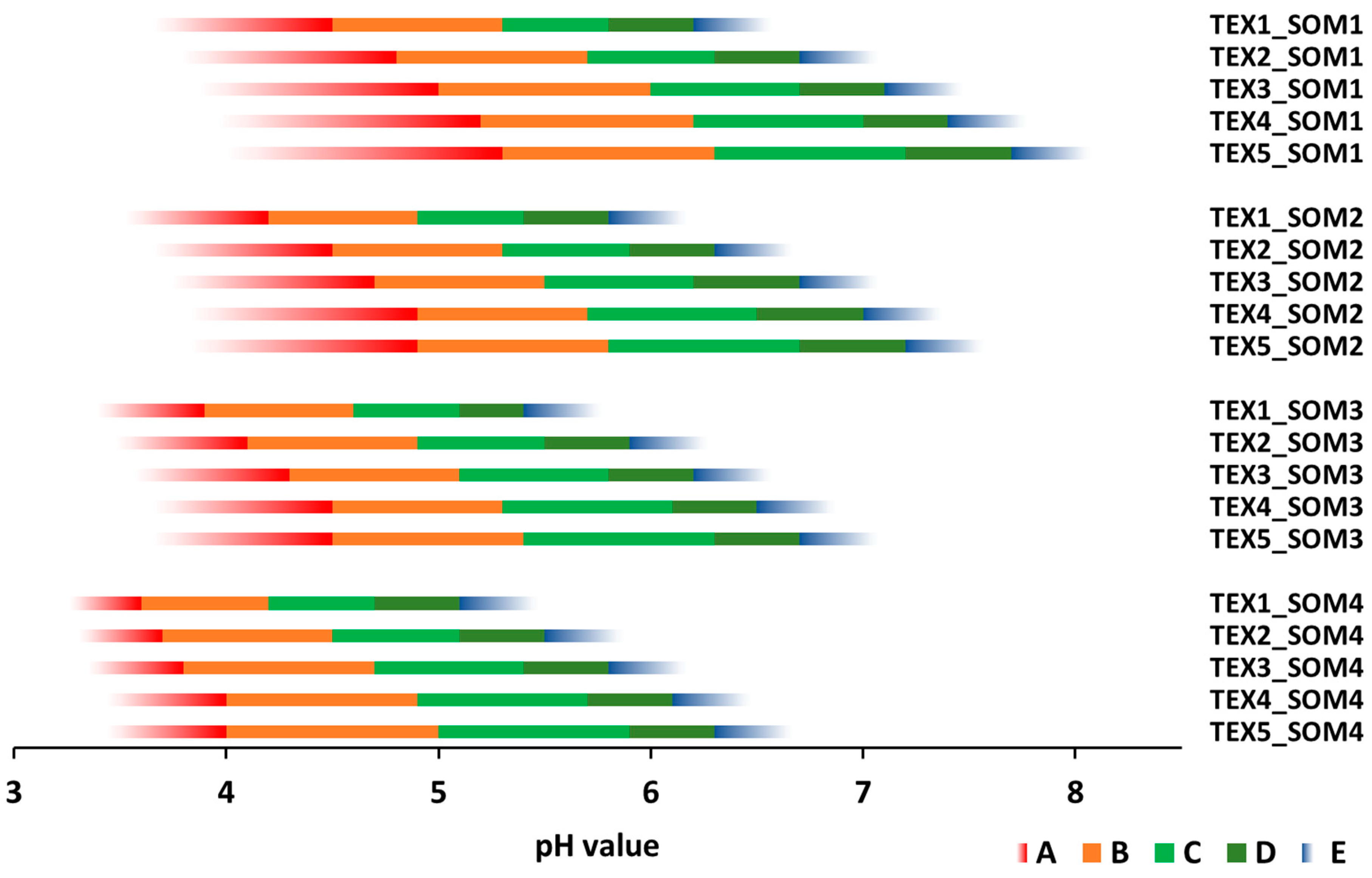
2.1.2. Dependency of the Lime Supply Status and of the Soil Lime Demand on Soil Texture, SOM Content and Soil pH

As mentioned in the description of the VDLUFA guidelines (see Introduction), the factors soil texture and the SOM content were identified as particularly relevant for the definition of optimum pH ranges, as well as of the CaO fertilizer amounts necessary to achieve the optimum soil pH range. The VDLUFA classification of the lime supply statuses (A to E) with pH ranges for the soil texture classes (TEX1 to TEX5) and the SOM classes (SOM1 to SOM4) are shown in Figure 1. The reported CaO application amounts necessary to reach the optimum lime supply as a function of the five soil texture classes, four SOM classes and the determined pH values are shown in Figure 2.

With regard to the lime supply conditions shown in Figure 1, the following dependencies can be derived:

• With an increasing clay content (TEX1 → TEX5), the ranges of the lime supply statuses (A–E) shift towards higher pH values and
• With an increasing SOM content (SOM1 → SOM4), the ranges of the lime supply statuses (A–E) shift towards lower pH values.

The relationships between the soil pH value and the recommended amount of CaO differ for the following three situations:

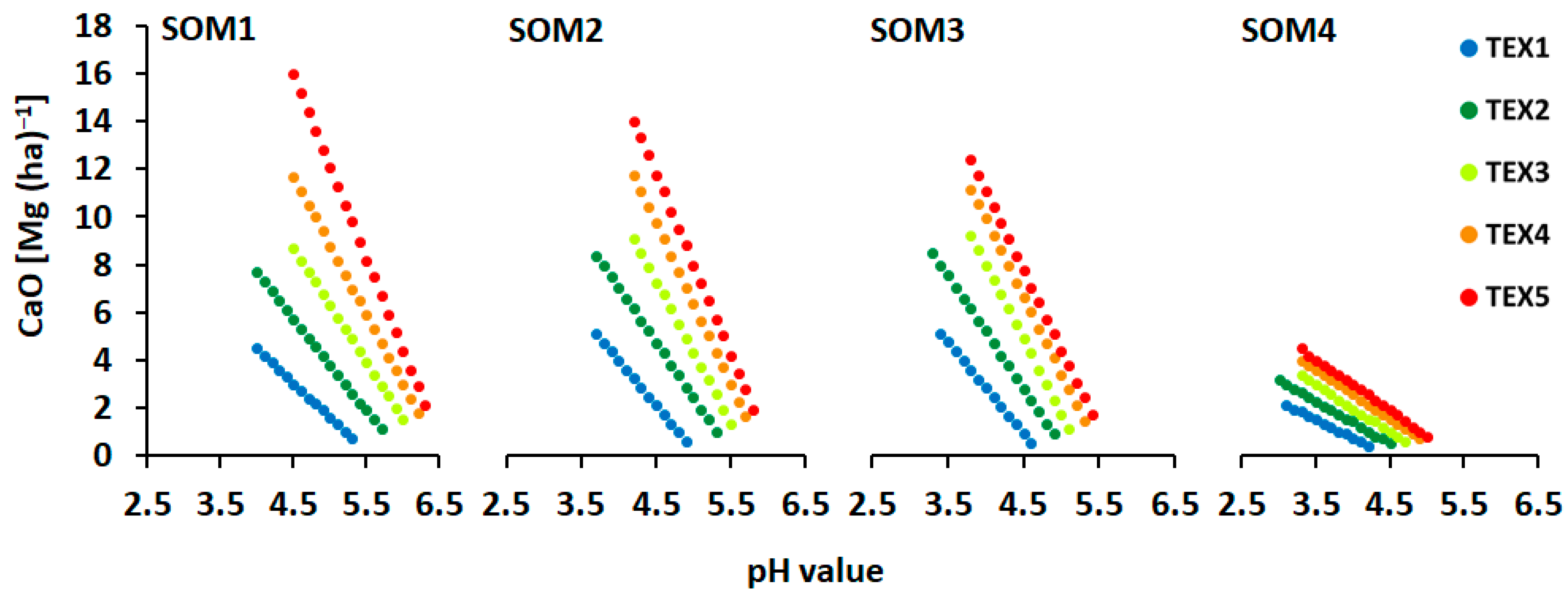
• Lime supply statuses A and B: the linear relationships between pH and the CaO demand as per each soil texture and SOM combination (Figure 2),
• Lime supply status C: fixed lime recommendations subdivided for the 20 soil texture and SOM combinations as shown in Figure 1 (Figure 3), and
• Lime supply statuses D and E: no lime demand

Under supply level statuses A and B, the pH is suboptimal. Therefore, the recommended amount of lime should increase the soil pH up to the optimum lime supply status C. As shown in Figure 2, the slopes of the linear functions decline more strongly with an increasing clay content (TEX1 → TEX5), while the intercepts increase. Under increasing SOM contents (SOM1 → SOM4), the mentioned behavior of the slopes and intercepts is opposed. Therefore, the task was to substitute the five soil texture classes and the four SOM classes with continuous scaled measures.

Within lime supply level C, the optimum pH range is already present. The recommended lime supplies preserve this level within a four-year crop rotation (Figure 1). However, the recommended CaO amounts by the VDLUFA approach are not further differentiated regarding the soil’s pH but are for each of the 20 combinations of soil texture and SOM class (Figure 3). The CaO amounts shown in Figure 3 are always lower than the lowest CaO amounts recommended for lime supply status B for each of the 20 combinations, but always higher than zero.

To avoid excessive application rates, the recommended maximum CaO amounts [Mg ha⁻¹] of a single application rate are merely soil texture dependent and vary as follows: TEX1 = 2.8, TEX2 = 4.2, TEX3 = 5.6, TEX4 = 7.0 and TEX5 = 8.4. When the recommended CaO amounts exceed these maxima, fertilization should be split into two rates and applied separately in time.

Under lime supply levels D and E, the pH values exceed the optimum pH range, and no liming is recommended to change the pH and achieve lime supply status C.

2.2. From the Stepwise, Class-Based VDLUFA Approach to a Stepless, Continuously Scaled Approach

Since the abovementioned VDLUFA approach is based on classified factors (five soil texture classes and four soil organic matter classes), transformation into continuously scaled soil textures and SOM contents is required.

The soil texture classification systems applied in Germany are mainly those of the German Soil Science Society (DBG) (31 soil texture classes) and the VDLUFA classification system (five soil texture classes). While the former is mainly used in a scientific context considering the three particle size fractions: clay (0–0.002 × 10⁻³ m), silt (0.002–0.063 × 10⁻³ m) and sand (0.063–2 × 10⁻³ m), the latter is solely based on the clay (or clay + fine silt) content and instead used in a practical background. However, to apply a continuously scaled soil texture measure under equal consideration of the clay, silt and sand fractions, this study refers to the geometric mean particle size diameter (MPD) according to Shiozawa and Campbell [24] as follows:

$$\mathrm{MPD}=exp{\displaystyle \sum }{m}_i \ln (d_i)$$

(1)

where MPD is given in [10⁻³ m], $m_i$ is the mass fraction of the particle size class i [kg kg⁻¹], and $d_i$ is the associated geometric mean diameter [10⁻³ m]. As suggested by Shirazi et al. [25], the lower limit of the clay size fraction was set to 1 × 10⁻⁸ m. The geometric means that correspond to the particle size class ranges of the clay, silt and sand fractions were 1.41 × 10⁻⁷ m, 1.12 × 10⁻⁵ and 3.55 × 10⁻⁴ m, respectively.

In the next step, the MPDs are calculated for the corresponding centroids of the polygons, as they represent the sand, silt and clay contents of the 31 DBG soil texture classes (

Table 2. Clay, silt, and sand contents [kg kg⁻¹] and the corresponding mean particle diameters (MPDs) [10⁻³ m] of the 31 DBG soil texture classes.

Soil Texture	Coordinate Centers of the Polygons
Classes	Clay	Silt	Sand	MPD
Tt	0.766	0.117	0.117	0.0006
Tu2	0.550	0.375	0.075	0.0013
Tl	0.550	0.225	0.225	0.0022
Tu3	0.363	0.563	0.074	0.0030
Tu4	0.284	0.683	0.033	0.0036
Ts2	0.550	0.075	0.375	0.0037
Lt3	0.400	0.400	0.200	0.0039
Ut4	0.210	0.720	0.070	0.0057
Lu	0.235	0.575	0.190	0.0077
Ut3	0.144	0.753	0.103	0.0085
Lt2	0.300	0.400	0.300	0.0085
Lts	0.350	0.225	0.425	0.0105
Ut2	0.100	0.775	0.125	0.0112
Uu	0.040	0.880	0.080	0.0124
Ts3	0.400	0.075	0.525	0.0120
Ls2	0.210	0.450	0.340	0.0145
Uls	0.125	0.575	0.300	0.0183
Ls3	0.210	0.350	0.440	0.0205
Ts4	0.300	0.075	0.625	0.0262
Us	0.040	0.650	0.310	0.0275
Slu	0.125	0.450	0.425	0.0282
Ls4	0.210	0.225	0.565	0.0315
Sl4	0.145	0.250	0.605	0.0481
St3	0.210	0.075	0.715	0.0529
Su4	0.040	0.450	0.510	0.0549
Sl3	0.100	0.250	0.650	0.0684
Su3	0.040	0.325	0.635	0.0845
Sl2	0.065	0.175	0.760	0.1166
St2	0.110	0.050	0.840	0.1262
Su2	0.025	0.175	0.800	0.1595
Ss	0.025	0.050	0.925	0.2456

). The classes of both the VDLUFA and DBG systems are shown in Figure 4.

Finally, the MPDs of the five VDLUFA soil groups are calculated from the corresponding arithmetic means of the DBG MPDs that lie within the uniform-colored areas of the respective VDLUFA soil groups (Figure 4). The five VDLUFA MPDs [10⁻³ m] are TEX1 = 0.203, TEX2 = 0.091, TEX3 = 0.042, TEX4 = 0.017 and TEX5 = 0.005.

Regarding the SOM classification, SOM classes 1–4 needed to be transferred into a continuously scaled measure as well. To calculate the corresponding continuous function, the arithmetic means of the abovementioned class ranges [g kg⁻¹]: SOM1 = 20, SOM2 = 60, SOM3 = 115, and SOM4 = 225 were used.

Applying this procedure allows us to characterize the five VDLUFA soil texture groups by their MPD and the four SOM groups by their mean SOM content. Based on these measures, the effects of the soil texture and the SOM could be calculated continuously for the lime supply statuses and the soil lime demand.

Aiming at the optimal lime supply status and going along with the stepless principles mentioned above, the task was to generate a continuously differentiated CaO determination that depends on the pH values within the lime supply levels A and B and that considers the pH range of lime supply status C. The latter was intended to the following manner: the lime recommendation should decrease linearly, beginning with the lowest CaO amount recommended in lime supply status B (CaOminB), down to zero where lime supply status D is reached.

2.3. Models and Statistics

Mathematical models were used to describe the lime supply statuses and the lime demand of the soil in relation to the MPD and mean SOM contents. The models were fitted with the software TableCurve 3D version 4.0 (SYSTAT). This surface fitting software package fits and ranks numerous equations automatically and finds the “ideal model” for any 3D data. The independent variables of our models were the MPD of the five texture classes and the mean SOM content of the four SOM classes, as mentioned above.

To determine the boundaries between the lime supply levels (A/B, B/C, C/D and D/E), the upper limits of the pH ranges of each lime supply level (pHmax_A–D) were chosen to fit the multidimensional mathematical models (Figure 1). The lime supply level E is >pHmax_D.

As described in Figure 2, 20 combinations between the five textures and the four SOM classes can be obtained to determine the lime demand according to VDLUFA. For each combination, the relationship between the observed pH (pH_obs) and the required lime demand (CaO) can be described with a simple linear function:

$$\mathrm{CaO}=m-n {\mathrm{pH}}_{\mathrm{obs}}$$

(2)

where m is the intercept and n the slope. Both m and n were assumed to be dependent on the soil texture and SOM. Therefore, first the 20 intercepts and then the 20 slopes were fitted in relation to the mean particle diameter MPD and the mean SOM content according to the respective classes.

The criterion for selecting the “ideal model” was that the function must be continuous—without local minima and maxima within the data range. Among these functions, the function with the best fit (highest R²) was selected. The aim of this procedure was to predict the lime supply statuses and the soil lime demand as exact and as close as possible to the class-based VDLUFA approach. Hence, the best model results should provide almost identical values compared to the original VDLUFA approach in order to avoid discrepancies, e.g., when agricultural service providers or farmers compare the outputs of our stepless approach with the VDLUFA look-up table system. Therefore, reducing the number of fitted model parameters and testing their level of significance were not criteria for selecting the respective model.

The algorithm to determine CaO amounts as stepless approach is provided as R-script of the free software environment for statistical computing and graphics R (version 4.0.2) [26] in the Supplementary Material.

3. Results

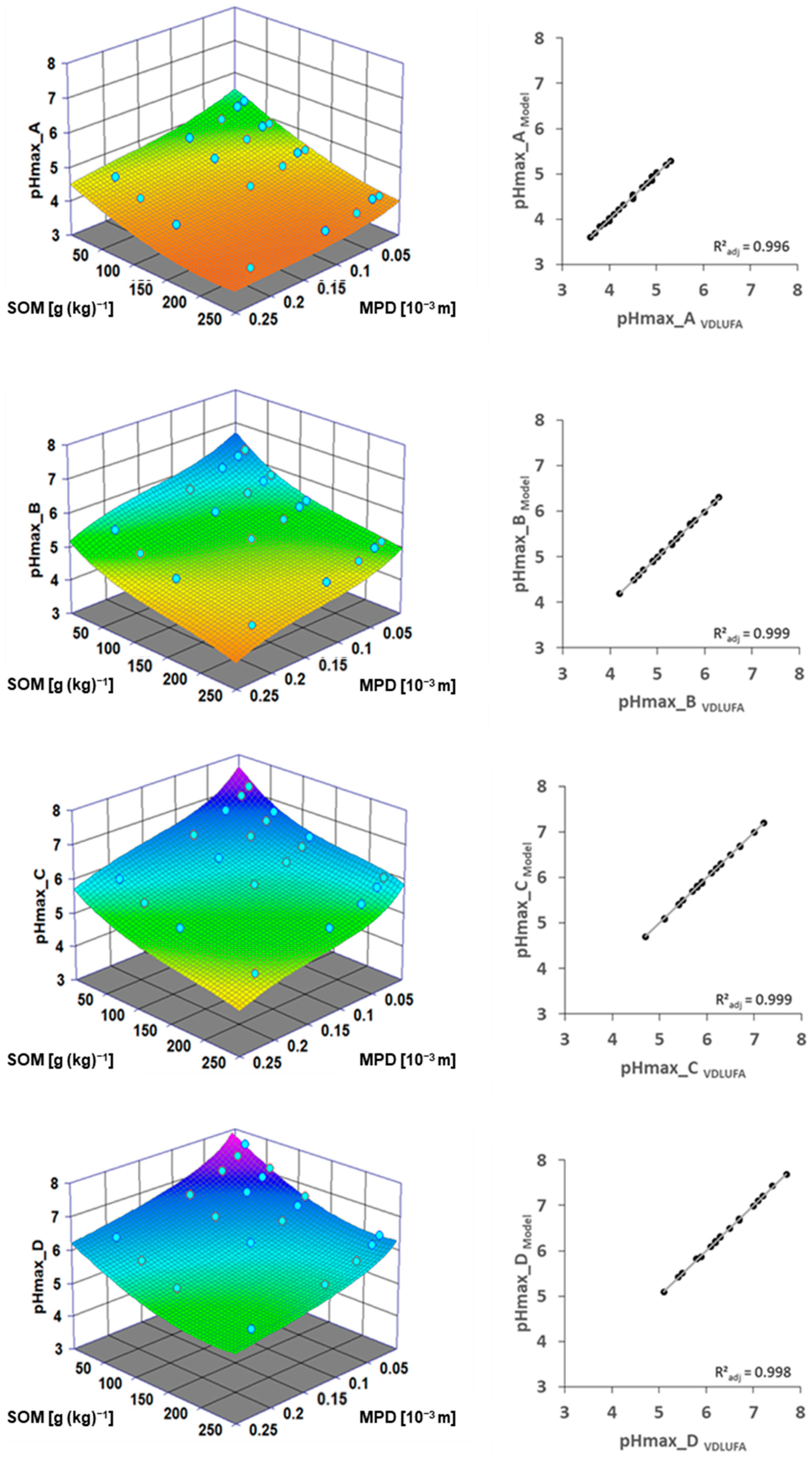
3.1. Predicting the Lime Supply Status of Soil

As mentioned in Section 2.1, the relationships between the soil pH and the recommended amount of CaO may differ if the present lime supply status is suboptimal (A or B), optimal (C) or exceeded (D or E). Therefore, the lime supply status as related to the MPDs and mean SOM contents (Figure 5) must be predicted first. The three-dimensional surfaces shown represent the boundaries of the lime supply levels (A/B, B/C, C/D and D/E) based on the maximum pH values of the lime supply levels A–D. The mathematical models that describe the three-dimensional relationships between the upper pH limits, the MPDs (x) and mean SOM contents (y) are given in Equations (3)–(6).

$$\begin{array}{c}\mathrm{pHmax\_A}=a+b\ast \ln \left(x\right)+c\ast y+d\ast {\left(\ln \left(x\right)\right)}^2+e\ast y^2+f\ast y\ast \ln \left(x\right)+g\\ \ast {\left(\ln \left(x\right)\right)}^3+h\ast y^3+i\ast y^2\ast \ln \left(x\right)+j\ast y\end{array}$$

(3)

$$\begin{array}{c}\mathrm{pHmax\_B}=a+b\ast x+c\ast y+d\ast x^2+e\ast y^2+f\ast x\ast y+g\ast x^3+h\ast y^3+i\\ \ast x\ast y^2+j\ast x^2\ast y\end{array}$$

(4)

$$\mathrm{pHmax\_C}=\frac{\left(a+b\ast x+c\ast x^2+d\ast y+e\ast y^2+f\ast y^3\right)}{\left(1+g\ast x+h\ast x^2+i\ast x^3+j\ast y\right)}$$

(5)

$$\begin{array}{c}\mathrm{pHmax\_D}=a+b\ast \ln \left(x\right)+c\ast y+d\ast {\left(\ln \left(x\right)\right)}^2+e\ast y^2+f\ast y\ast \ln \left(x\right)+g\\ \ast {\left(\ln \left(x\right)\right)}^3+h\ast y^3+i\ast y^2\ast \ln \left(x\right)+j\ast y\end{array}$$

(6)

where pHmax_(A–D) are the upper limits of the pH range for each lime supply status A–D, a–j are fitting coefficients.

The adjusted coefficients corresponding to the models are then listed in

Table 3. Fitted coefficients and their standard errors (in parentheses) of the mathematical models, as shown in Equations (3)–(6).

Fitted	Dependent Variable
Coefficient	pHmax_A 1	pHmax_B 1	pHmax_C 1	pHmax_D 1
a	4.13	6.69	7.64	4.87
	(1.85 × 10−1)	(2.19 × 10−2)	(2.22 × 10−2)	(1.38 × 10−1)
b	−2.37 × 10−1	−1.17 × 10	1.08 × 10	−1.15
	(1.75 × 10−1)	(7.19 × 10−1)	(5.58)	(1.30 × 10−1)
c	−5.17 × 10−3	−1.81 × 10−2	−1.03 × 10	−8.26 × 10−3
	(1.90 × 10−3)	(8.02 × 10−4)	(1.66 × 10)	(1.41 × 10−3)
d	7.34 × 10−2	6.31 × 10	−3.04 × 10−2	−1.33 × 10−1
	(5.32 × 10−2)	(9.56)	(3.28 × 10−3)	(3.96 × 10−2)
e	5.31 × 10−6	7.94 × 10−5	1.05 × 10−4	9.51 × 10−6
	(1.69 × 10−5)	(8.53 × 10−6)	(1.02 × 10−5)	(1.26 × 10−5)
f	1.72 × 10−3	1.74 × 10−2	−1.95 × 10−7	1.46 × 10−3
	(5.06 × 10−4)	(3.77 × 10−3)	(2.55 × 10−8)	(3.77 × 10−4)
g	1.34 × 10−2	−1.63 × 10−2	4.28	−4.79 × 10−3
	(5.09 × 10−3)	(3.22 × 10)	(7.76 × 10−1)	(3.79 × 10−3)
h	3.00 × 10−8	−1.39 × 10−7	−1.49 × 10	3.54 × 10−8
	(4.66 × 10−8)	(2.41 × 10−8)	(1.97)	(3.47 × 10−8)
i	−9.94 × 10−8	−5.60 × 10−5	3.62 × 10	−1.83 × 10−6
	(1.15 × 10−6)	(1.08 × 10−5)	(7.56)	(8.60 × 10−7)
j	1.78 × 10−4	7.68 × 10−3	−1.55 × 10−3	9.13 × 10−5
	(5.87 × 10−5)	(1.20 × 10−2)	(4.00 × 10−4)	(4.38 × 10−5)

¹ pHmax_A–D = upper limits of the pH range for each lime supply status A–D.

. The models were able to describe these continuous relationships almost perfectly (R² > 0.99 in each case) when the predicted values were compared with those of the VDLUFA approach.

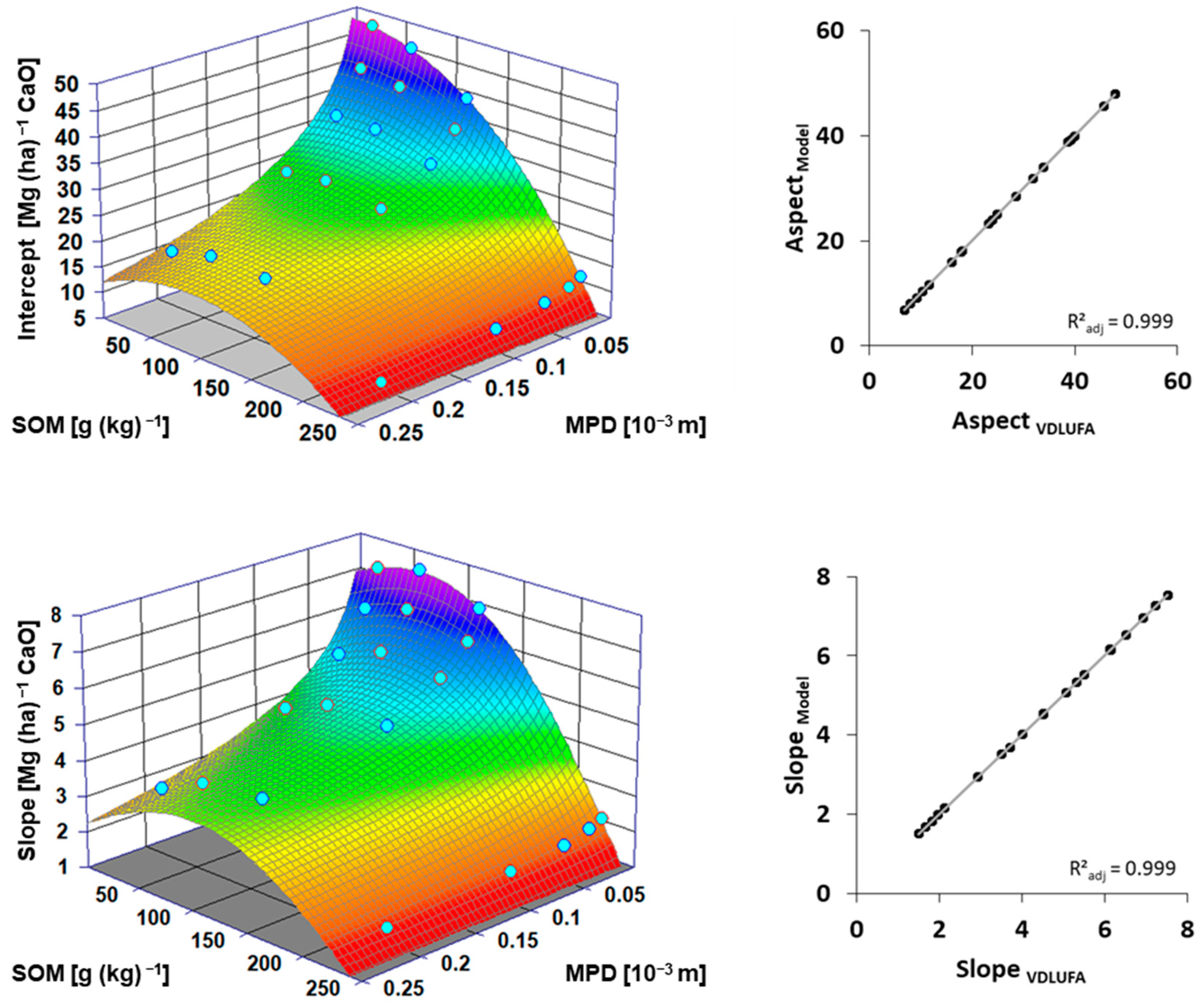
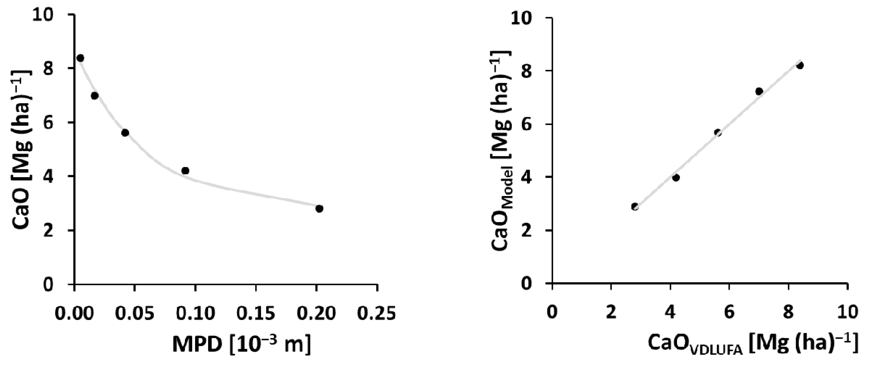
3.2. Predicting the Lime Demand of Soils for Different Lime Supply Statuses

Regarding lime supply statuses A and B, the 20 linear relationships between the soil pH and the lime demand are dependent on soil texture and SOM, as shown in Figure 2. Here, both the intercepts and the slopes of the corresponding linear relationships are related to the MPDs of the five VDLUFA soil texture classes and to the mean SOM contents of the four VDLUFA SOM classes (Figure 6).

The mathematical models that describe the three-dimensional relationships between the intercepts or slopes, the MPDs (x) and mean SOM contents (y) are given in Equations (7)–(8).

$$\mathrm{intercept}=\frac{(a+c\ast \ln \left(x\right)+e\ast y+g\ast {\left(\ln \left(x\right)\right)}^2+i\ast y^2+k\ast y\ast \ln \left(x\right)}{(1+b\ast \ln \left(x\right)+d\ast y+f\ast {\left(\ln \left(x\right)\right)}^2+h\ast y^2+j\ast y\ast \ln \left(x\right)}$$

(7)

$$\mathrm{slop}=\frac{(a+c\ast \ln \left(x\right)+e\ast y+g\ast {\left(\ln \left(x\right)\right)}^2+i\ast y^2+k\ast y\ast \ln \left(x\right)}{(1+b\ast \ln \left(x\right)+d\ast y+f\ast {\left(\ln \left(x\right)\right)}^2+h\ast y^2+j\ast y\ast \ln \left(x\right)}$$

(8)

where a–j fitting coefficients.

The adjusted coefficients corresponding to these models are then listed in

Table 4. Fitted coefficients and their standard errors (in parentheses) of the mathematical models, as shown in Equations (7) and (8).

Fitted	Dependent Variable
Coefficient	Intercept 1	Slope 1
a	−1.32	4.69 × 10−1
	(8.96 × 10−2)	(2.93 × 10−2)
b	1.01 × 10−1	8.20 × 10−2
	(1.80 × 10−3)	(4.64 × 10−3)
c	−8.64	−1.12
	(7.29 × 10−2)	(2.72 × 10−2)
d	4.39 × 10−4	−1.75 × 10−3
	(5.96 × 10−5)	(1.57 × 10−4)
e	1.45 × 10−1	2.24 × 10−2
	(1.50 × 10−3)	(6.35 × 10−4)
f	1.70 × 10−2	1.44 × 10−2
	(1.50 × 10−4)	(3.83 × 10−4)
g	3.71 × 10−2	1.28 × 10−2
	(4.79 × 10−3)	(1.59 × 10−3)
h	−7.33 × 10−7	7.71 × 10−6
	(1.47 × 10−7)	(5.18 × 10−7)
i	−5.18 × 10−4	−8.45 × 10−5
	(5.22 × 10−6)	(2.40 × 10−6)
j	2.22 × 10−4	2.08 × 10−4
	(5.89 × 10−6)	(1.20 × 10−5)
k	3.64 × 10−2	5.02 × 10−3
	(2.73 × 10−4)	(9.57 × 10−5)

¹ Intercept and slope of the relationship between the pH and lime demand.

. The models were able to describe these continuous relationships almost perfectly (R² > 0.99 in each case) when the predicted values were compared with those of the VDLUFA approach (Figure 6, right).

To avoid excessive CaO applications, very high recommended CaO amounts should be split into two application rates. As recommended by the VDLUFA approach and mentioned in Section 2.1, the maximum amounts of a single CaO application (CaOmax) are merely soil texture dependent. By considering the soil texture classes by their corresponding MPDs, the relationship can be expressed by an exponential function that reads as follows (Figure 7):

$$\mathrm{CaO}max=\left(r-s\right)\ast \left(exp\left(-t\ast \mathrm{MPD}\right)\right)+s$$

(9)

where CaOmax is the maximum CaO application rate [Mg ha⁻¹], MPD = mean particle diameter [10⁻³ m] and r, s and t are dimensionless coefficients that have the following values (standard deviations): 8.7 (0.4), 2.7 (0.4) and 16.8 (3.2), respectively.

Regarding the lime supply status C, the task was to relate the lime recommendation linearly to the pH, decreasing from the lowest CaO amount recommended in lime supply status B to zero as recommended if the pH achieves lime supply status D. Therefore, the upper pH limits of the lime supply statuses B (pHmax_B) and C (pHmax_C) were applied according to Equations (4) and (5). The minimum CaO demand (CaOmin_B) of lime supply level B, which refers to its maximum pH (pHmax_B), can be calculated from Equations (2), (7) and (8). The CaO demand, which refers to the maximum pH of supply level C (pHmax_C), was set to 0 Mg CaO/ha. Consequently, the CaO demand (CaO_C) for any given pH (pHobs_C) will be calculated in our approach as follows:

$$\mathrm{CaO\_C}=\mathrm{CaOmin\_B}\ast \left(\left(\mathrm{pHmax\_C}-\mathrm{pHobs\_C}\right)\right)/\left(\left(\mathrm{pHmax\_C}-\mathrm{pHmax\_B}\right)\right)$$

(10)

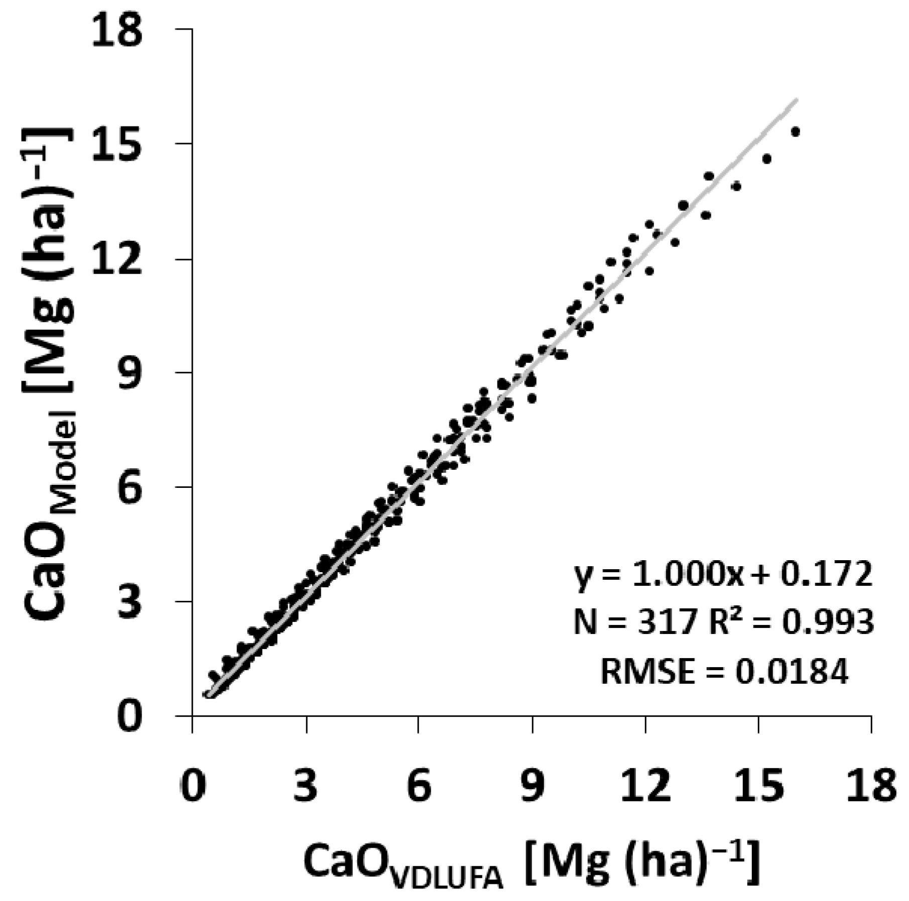
3.3. Model Validation

Equation (2) can be used to describe the intercept and the slopes of the linear relationships between the soil’s pH and lime demand for each of the 20 combinations of the soil texture and SOM classes. The dependencies of the intercepts (Equation (7)) and the slopes (Equation (8)) of these 20 linear functions from the MPD and SOM content are shown in Figure 6. Based on these dependencies, intercepts and slopes can be calculated steplessly for each combination between the pH value, soil texture (expressed as MPD, which is based on the clay, silt and sand content) and the SOM content within the data ranges given in Section 2.1.

To validate the stepless approach, the results were compared with the CaO recommendations provided by the VDLUFA look-up table system (n = 317) for pH values that correspond to lime supply statuses A and B (Figure 8).

The calculation of the soil lime demand based on the results shown in Figure 6 resulted in excellent model performance. Less than 0.01% of the variability in the CaO amount which is recommended by the VDLUFA approach cannot be explained by the stepless approach.

4. Discussion

The VDLUFA look-up table system [16] predicts the lime demand of soils as class-based, dependent on soil texture and the SOM. It is advantageous for farmers because they can apply it without calculations or special expert knowledge. On the other hand, the subdivision of the soil texture and the SOM into classes is a limitation if applied in a precision farming context. Using modern sensor-based soil mapping techniques, which can provide detailed, highly spatially resolved soil texture and SOM maps, a transformation from the class-based system into a continuous, stepless approach is necessary. As shown in our approach, the transformation from the class-based look-up table system to a continuous, stepless approach succeeded. In the results, we could explain more than 99% of the variability of the 317 recommended CaO amounts for lime supply statuses A and B, differentiating into five soil texture classes and four organic matter classes. Regarding the chosen mathematical models, our focus was to predict these 317 recommended CaO amounts as exactly as possible by the models allying to the continuous approach—without local minima and maxima and within the data range. Neither reducing the number of fitted model parameters nor testing for their level of significance were criteria for selecting the respective model.

Compared to other international approaches [13,27,28], the German VDLUFA agricultural liming recommendation is the most detailed and considers not only the influence of pH but also the effects of soil texture and SOM. Therefore, the applied methodology may be of broader interest, especially because algorithms that are needed in the context of present-day requirements of precision farming should be continuous and stepless. However, to derive the maximum benefit from the continuous liming approach, the following problems that are obvious within the chain-from the primary data acquisition (pH, soil texture, SOM) to the final lime spreading-need to be considered:

• The finger texturing method is usually applied for agricultural purposes because the exact estimation of the soil texture by sieving and sedimentation analyses is time- and cost-intensive. However, Stocker and Walthert [29] reported that solely 68%, 31% and 56% of clay, silt and sand variability, respectively, could be explained by the finger texturing method (predicted by sieving and sedimentation analyses). They took more than 11,000 soil samples from approximately 90 Swiss forest sites from six depth levels down to 1.5 m. This rather imprecise soil texture determination can lead to unrealistic and severe differences in the lime application recommendations of management units [19].
• In the past, management zones of 3 to 5 ha with assumed homogenous soil were chosen, since equal zones generally require the same liming rates and provide reasonable sizes in terms of the application equipment and sampling rates [30]. However, the creation of those management zones neglects the variation in the soil texture, SOM and the actual pH within the management units. To provide reliable soil parameters for lime management at a higher spatial resolution and low costs, on-the-go soil sensor systems, such as the Geophilus [31] and the Veris pH manager [32], are appropriate solutions. Meyer et al. [19] used the mentioned sensor systems in combination with targeted soil samples that were taken for sensor calibrations by analyzing the soil pH, SOM and soil texture with standardized laboratory methods. Finally, they produced 2 × 2 m maps of the actual soil acidity (pH), SOM and soil texture (clay, silt, and sand). Bönecke et al. [17] used these generated soil maps and the stepless algorithm to successfully produce variable rate lime application maps. They compared the variable liming rates with a standard uniform liming approach and found that 63% of the field would be over-fertilized by approximately 12 Mg of lime, 6% would receive approximately 6 Mg too little lime and 31% would still be adequately limed under the uniform liming approach.
• As mentioned above, reference or targeted soil sampling is necessary to calibrate sensor data that are not causally related to the agronomic parameters used to make management decisions. In practice, the determination of sampling locations is almost subjective. According to Adamchuk et al. [33], three criteria should be considered: (a) targeted samples have to cover the entire range of the sensor data, (b) within a radius of 30 m around the reference sampling point, the soil should be spatially homogeneous and (c) the targeted sampling locations should be well distributed throughout the area of investigation. To the best of our knowledge, a reliable automated approach to determine the targeted sampling locations built up on these three criteria is still missing.
• Regarding fertilizer applicators, Lawrence [21,34,35] reported that, although variable rate technologies have been demonstrated to satisfactorily operate the actual performance of the fertilizer, spreading machinery is often shown to be inadequate. A similar assessment was given by Holmes and Jiang [36] who argued that the current fertilizer spreading equipment does not provide the accuracy needed to undertake variable rate liming trials. This problem is further aggravated because the two main variable rate fertilizer application techniques are the application of liquid and granulose products. Granular lime fertilizers are available, but are more expensive and therefore usually less applied.

Regardless of the presented problems, increasing attention is being paid to small-scale site-adapted liming by farmers, not least because it is associated with three kinds of benefits: agronomical, economic and environmental.

References

1. Pierce, F.J.; Nowak, P. Aspects of Precision Agriculture. In Advances in Agronomy; Elsevier: Amsterdam, The Netherlands, 1999; Volume 67, pp. 1–85. [Google Scholar]
2. Basso, B.; Cammarano, D.; Fiorentino, C.; Ritchie, J.T. Wheat yield response to spatially variable nitrogen fertilizer in Mediterranean environment. Eur. J. Agron. 2013, 51, 65–70. [Google Scholar] [CrossRef]
3. Robertson, M.J.; Llewellyn, R.S.; Mandel, R.; Lawes, R.; Bramley, R.G.V.; Swift, L.; Metz, N.; O’Callaghan, C. Adoption of variable rate fertiliser application in the Australian grains industry: Status, issues and prospects. Precis. Agric. 2012, 13, 181–199. [Google Scholar] [CrossRef]
4. Robert, P.C. Precision agriculture: A challenge for crop nutrition management. In Progress in Plant Nutrition: Plenary Lec-Tures of the XIV International Plant Nutrition Colloquium: Food Security and Sustainability of Agro-ecosystems through Basic and Applied Research; Horst, W.J., Ed.; Kluwer Academic Publishers: Dordrecht, The Netherlands, 2010; pp. 143–149. ISBN 978-90-481-6191-1. [Google Scholar]
5. Moharana, P.C.; Jena, R.K.; Pradhan, U.K.; Nogiya, M.; Tailor, B.L.; Singh, R.S.; Singh, S.K. Geostatistical and fuzzy clustering approach for delineation of site-specific management zones and yield-limiting factors in irrigated hot arid environment of India. Precis. Agric. 2019, 21, 426–448. [Google Scholar] [CrossRef]
6. Moral, F.J.; Rebollo, F.J.; Serrano, J.M. Delineating site-specific management zones on pasture soil using a probabilistic and objective model and geostatistical techniques. Precis. Agric. 2019, 21, 620–636. [Google Scholar] [CrossRef]
7. Wang, X.; Miao, Y.; Dong, R.; Chen, Z.; Kusnierek, K.; Mi, G.; Mulla, D.J. Economic Optimal Nitrogen Rate Variability of Maize in Response to Soil and Weather Conditions: Implications for Site-Specific Nitrogen Management. Agronomy 2020, 10, 1237. [Google Scholar] [CrossRef]
8. Basso, B.; Dumont, B.; Cammarano, D.; Pezzuolo, A.; Marinello, F.; Sartori, L. Environmental and economic benefits of variable rate nitrogen fertilization in a nitrate vulnerable zone. Sci. Total Environ. 2016, 545–546, 227–235. [Google Scholar] [CrossRef] [Green Version]
9. Nawar, S.; Corstanje, R.; Halcro, G.; Mulla, D.; Mouazen, A.M. Delineation of Soil Management Zones for Variable-Rate Fertilization. In Advances in Agronomy; Elsevier: Amsterdam, The Netherlands, 2017; pp. 175–245. [Google Scholar]
10. Vogel, S.; Bönecke, E.; Kling, C.; Kramer, E.; Lück, K.; Nagel, A.; Philipp, G.; Rühlmann, J.; Schröter, I.; Gebbers, R. Base Neutralizing Capacity of Agricultural Soils in a Quaternary Landscape of North-East Germany and Its Relationship to Best Management Practices in Lime Requirement Determination. Agronomy 2020, 10, 877. [Google Scholar] [CrossRef]
11. Schilling, G.; Ansorge, H. Pflanzenernährung und Düngung: 164 Tabellen (Plant Nutrition and Fertilization: 164 Tables); VEB Deutscher Landwirtschaftsverlag: Berlin, Germany, 1982. (In German) [Google Scholar]
12. Blume, H.-P.; Brümmer, G.W.; Horn, R.; Kandeler, E.; Kögel-Knabner, I.; Kretzschmar, R.; Stahr, K.; Wilke, B.-M.; Thiele-Bruhn, S.; Welp, G. Scheffer/Schachtschabel: Lehrbuch der Bodenkunde (Scheffer/Schachtschabel: Textbook of Soil Science); Springer: Berlin/Heidelberg, Germany, 2010. [Google Scholar]
13. Goulding, K.W.T. Soil acidification and the importance of liming agricultural soils with particular reference to the United Kingdom. Soil Use Manag. 2016, 32, 390–399. [Google Scholar] [CrossRef]
14. Kerschberger, M.; Deller, B.; Hege, U.; Heyn, J.; Kape, H.E.; Krause, O.; Pollehn, J.; Rex, M.J.; Severin, K. Bestimmung des Kalkbedarfs von Acker-Und Grünlandböden (Determination of the Lime Requirement of Arable and Grassland Soils); VDLUFA-Verlag: Speyer, Germany, 2000. [Google Scholar]
15. Kerschberger, M.; Marks, G. Einstellung und Erhaltung eines standorttypischen optimalen pH-Wertes im Boden-Grundvoraussetzung fur eine effektive und umweltvertragliche Pflanzenproduktion (Setting and maintaining a site-specific optimum pH value in the soil-a basic requirement for effective and environmentally compatible plant production). Berichte über Landwirtschaft 2007, 85, 56–77. [Google Scholar]
16. Von Wulffen, U.; Roschke, M.; Kape, H.-E. Richtwerte für die Untersuchung und Beratung Sowie zur Fachlichen Umsetzung der Düngeverordnung (DüV): Gemeinsame Hinweise der Länder Brandenburg, Mecklenburg-Vorpommern und Sachsen-Anhalt (Guide values for the Examination and Advice as Well as for the Professional Implementation of the Fertilizer Ordinance (DüV): Joint Information from the States of Brandenburg, Mecklenburg-Western Pomerania and Saxony-Anhalt); LLFG: Güterfelde, Germany, 2008. [Google Scholar]
17. Bönecke, E.; Meyer, S.; Vogel, S.; Schröter, I.; Gebbers, R.; Kling, C.; Kramer, E.; Lück, K.; Nagel, A.; Philipp, G.; et al. Guidelines for precise lime management based on high-resolution soil pH, texture and SOM maps generated from proximal soil sensing data. Precis. Agric. 2020, 1–31. [Google Scholar] [CrossRef]
18. Boenecke, E.; Lueck, E.; Ruehlmann, J.; Gruendling, R.; Franko, U. Determining the within-field yield variability from seasonally changing soil conditions. Precis. Agric. 2018, 19, 750–769. [Google Scholar] [CrossRef]
19. Meyer, S.; Kling, C.; Vogel, S.; Schröter, I.; Nagel, A.; Kramer, E.; Gebbers, R.; Philipp, G.; Lück, K.; Gerlach, F.; et al. Creating soil texture maps for precision liming using electrical resistivity and gamma ray mapping. In Precision Agriculture’19; Wageningen Academic Publishers: Wageningen, The Netherlands, 2019. [Google Scholar]
20. Haynes, R.; Naidu, R. Influence of lime, fertilizer and manure applications on soil organic matter content and soil physical conditions: A review. Nutr. Cycl. Agroecosyst. 1998, 51, 123–137. [Google Scholar] [CrossRef]
21. Lawrence, H.G. Adoption of Precision Agriculture Technologies for Fertiliser Placement in New Zealand. Ph.D. Thesis, Massey University, Palmerston North, New Zealand, 2007. [Google Scholar]
22. Fulton, J.P.; Shearer, S.A.; Chabra, G.; Higgins, S.F. Performance Assessment and Model Development of A Variable–Rate, Spinner–Disc Fertilizer Applicator. Trans. ASAE 2001, 44, 1071. [Google Scholar] [CrossRef]
23. Voon Wulffen, H.-U.; Horn, D.; Lorenz, F.; Müller, R.; Müller, T.; Münchhoff, K.; Pihl, U.; Weber, A. DLG-Merkblatt 456—Hinweise zur Kalkdüngung (DLG-Leaflet 456—Notes on Lime Fertilization), 1st ed.; DLG e. V.: Frankfurt am Main, Germany, 2020. [Google Scholar]
24. Shiozawa, S.; Campbell, G.S. On The Calculation of Mean Particle Diameter and Standard Deviation from Sand, Silt, and Clay Fractions. Soil Sci. 1991, 152, 427–431. [Google Scholar] [CrossRef]
25. Shirazi, M.A.; Boersma, L.; Hart, J.W. A Unifying Quantitative Analysis of Soil Texture: Improvement of Precision and Extension of Scale. Soil Sci. Soc. Am. J. 1988, 52, 181–190. [Google Scholar] [CrossRef]
26. R Core Team. R: A Language and Environment for Statistical Computing; R Foundation for Statistical Computing: Vienna, Austria, 2018; Available online: https://www.R-project.org (accessed on 17 August 2020).
27. Baumgarten, A.; Berthold, H.; Buchgraber, K.; Dersch, G.; Egger, H.; Egger, R.; Eigner, H.; Frank, P.; Gerzabek, M.; Hölzl, F.X. Richtlinie für die Sachgerechte Düngung im Ackerbau und Grünland (Guideline for Appropriate Fertilization in Arable Farming and Grassland); BMLFUW: Wien, Austria, 2017. [Google Scholar]
28. Vitosh, M.L.; Johnson, J.W.; Mengel, D.B. Tri-State Fertilizer Recommendations for Corn, Soybean, Wheat and Alfalfa; Extension Bulletin; Ohio State University: Columbus, OH, USA, 1995; E-2567; Available online: http://ohioline.osu.edu/e2567/ (accessed on 23 January 2021).
29. Stocker, N.; Walthert, L. Böden und Wasserhaushalt von Wäldern und Waldstandorten der Schweiz unter heutigem und zukünftigem Klima (BOWA-CH)—Datengrundlage und Datenharmonisierung. (Soils and Water Balance of Forests and Forest Locations in Switzerland under Current and Future Climates—Data Basis and Data Harmonization) Projektinterner Bericht (Internal Project Report); ETH-Zurich: Zurich, Switzerland, 2013. [Google Scholar]
30. Borgelt, S.C.; Searcy, S.; Stout, B.A.; Mulla, D.J. Spatially Variable Liming Rates: A Method for Determination. Trans. ASAE 1994, 37, 1499–1507. [Google Scholar] [CrossRef]
31. Lueck, E.; Ruehlmann, J. Resistivity mapping with GEOPHILUS ELECTRICUS—Information about lateral and vertical soil heterogeneity. Geoderma 2013, 199, 2–11. [Google Scholar] [CrossRef]
32. Schirrmann, M.; Gebbers, R.; Kramer, E.; Seidel, J. Soil pH Mapping with an On-The-Go Sensor. Sensors 2011, 11, 573–598. [Google Scholar] [CrossRef]
33. Adamchuk, V.I.; Rossel, R.A.V.; Marx, D.B.; Samal, A.K. Using targeted sampling to process multivariate soil sensing data. Geoderma 2011, 163, 63–73. [Google Scholar] [CrossRef]
34. Lawrence, H.G.; Yule, I.J. A GIS Methodology to Calculate In-Field Dispersion of Fertilizer from a Spinning-Disc Spreader. Trans. ASABE 2007, 50, 379–387. [Google Scholar] [CrossRef]
35. Lawrence, H.G.; Yule, I.J.; Coetzee, M.G. Development of an Image-Processing Method to Assess Spreader Performance. Trans. ASABE 2007, 50, 397–407. [Google Scholar] [CrossRef]
36. Holmes, A.W.; Jiang, G. Effect of variable rate lime application on autumn sown barley performance. Agron. N. Z. 2017, 47, 37–45. [Google Scholar]
Figure 1. pH ranges of the lime supply statuses A–E (compare Table 1) in relation to the soil texture classes (TEX1–5) and the soil organic matter (SOM) classes (SOM1–4).
Agronomy 11 00785 g001
Figure 2. CaO amounts recommended by VDLUFA to increase the pH value from suboptimal statuses to the optimum pH ranges, depending on the SOM and soil texture classes. The given pH ranges correspond to the lime supply statuses A and B (compare Table 1 and Figure 1). The recommendation is usually related to a period of 4 years (one crop rotation).
Agronomy 11 00785 g002
Figure 3. CaO amounts to maintain the optimum pH range (lime supply status C) depending on the soil texture classes and soil organic matter classes. These VDLUFA recommendations refer to a crop rotation of 4 years.
Agronomy 11 00785 g003
Figure 4. Soil texture classes of VDLUFA (TEX1 = yellow, TEX2 = ochre yellow, TEX3 = brown, TEX4 = green, TEX5 = blue) and 31 German Soil Science Society (DBG) soil texture classes (polygons with labeled centroid points (black dots)) as related to the clay and silt contents.
Agronomy 11 00785 g004
Figure 5. Left: Upper pH limits of the lime supply statuses (pHmax_A–D) as used by the VDLUFA approach (dots) and calculated according to Equations (3)–(6) (surfaces), always in relation to the soil organic matter (SOM) content and the mean particle diameter (MPD). Right: maximum pH values as predicted by Equations (3)–(6) (pHmax_A–D Model) vs. the observed pH values by the VDLUFA approach (pHmax_A–D VDLUFA).
Agronomy 11 00785 g005
Figure 6. Left: Intercepts (top) and slopes (bottom) of the dependency of the CaO demand of soils on the soil pH, mean particle diameter (MPD) and soil organic matter (SOM) content as calculated based on the linear relationships given by the VDLUFA approach and shown in Figure 2 (dots) and calculated according to Equations (7) and (8) (surfaces). Right: Intercepts (top) and slopes (bottom) calculated by Equations (7) and (8), respectively, predicted (Model) vs. observed (VDLUFA) approach.
Agronomy 11 00785 g006
Figure 7. (Left): Maximum amount of a single CaO application [Mg ha−1] as recommended by the VDLUFA approach (dots) and calculated according to Equation (9) (line) always in relation to the mean particle diameter (MPD) [10−3 m]. (Right): CaO amounts predicted by Equation (9) (CaOModel) vs. observed VDLUFA (CaOVDLUFA); R2 = 0.992.
Agronomy 11 00785 g007
Figure 8. CaO amounts necessary to increase the pH value from a suboptimal range (lime supply statuses A and B) to the optimum pH range (lime supply status C), as recommended by the VDLUFA approach (CaOVDLUFA, see Figure 3), in comparison to the CaO amounts predicted by the stepless approach (CaOModel).
Agronomy 11 00785 g008