
A Control Method Based on a Simple Dynamic Optimizer: An Application to Micromachines with Friction

Department of Mathematics, ESEIAAT-Universitat Politècnica de Catalunya, 08222 Terrassa, Spain
Micromachines 2023, 14(2), 387; https://doi.org/10.3390/mi14020387
Submission received: 15 November 2022
/
Revised: 2 February 2023
/
Accepted: 2 February 2023
/
Published: 4 February 2023
(This article belongs to the Special Issue Controls of Micromachines)
Abstract
:In Micromachines, like any mechanical system, friction compensation is an important topic for control design application. In real applications, a nonlinear control scheme has proven to be an efficient method to mitigate the effects of friction. Therefore, a new regulation control method based on a simple dynamic optimizer is proposed. The used optimizer has a finite-time convergence to the optimal value of a given performance index. This dynamic process is then modified to produce a new control scheme to resolve the regulation control statement. A stability test is also provided along with numerical simulations to support our approach. We used the Lyapunov theory to confirm the stability, in finite-time, of the obtained closed-loop system. Furthermore, we tested this controller in a scenario where the reference signal was a time-varying function applied to a micromachine with friction. Numerical experiments showed acceptable performance in mitigating the effects of friction in the mechanism. In the simulations, the well-known LuGre friction model was invoked.
1. Introduction
Micromachines for micro-position control using piezoelectric actuators have been an important technology in some precision engineering applications [1,2,3]. Piezoelectric actuators are commonly used in micromachine control due to their infinite displacement resolution and low heat generation, among other factors [1,3]. However, these actuators exhibit hysteretic friction, which plays an important role in control design [1,3,4]. Regarding this point, many control strategies have been proposed. Among these, we have those based on PID schemes [3], modern control theory [2], robust analysis [5,6], neuronal theory together with terminal sliding mode control [7], and so on. Here, we propose a new control scheme based on a kind of dynamic optimizer [8].
For several years, control design using optimal mathematical tools has been a well-known control theory approach [9,10,11]. Even so, among the different methods, the extremum seeking technique remains a current control methodology in some engineering applications [12,13,14]. This control approach has gained considerable popularity after the publication cited in [15]. Essentially, the extremum seeking control scheme was proposed as a tool for model-less stable dynamical systems [16]. It is well known that real-time optimization integrated into a control scheme can improve closed-loop system performance. Furthermore, it can also help stabilize an unstable system [17]. A disadvantage of this technique is that it requires a disturbance signal [13]. This limits the convergence of the system and complicates the adjustment of the control system parameters [13]. On the other hand, a dynamic optimizer with convergence in finite-time was given in [8]. This optimizer did not require any disturbance signal. Therefore, the main objective of this article was to adapt this scheme to a dynamic system and satisfy the regulation control problem statement. We used Lyapunov theory for the finite-time stability test. In addition, numerical experiments were carried out to support our main contribution. For the numerical experimentation we used the application of the software. Both regulation and tracking control issues were numerically analyzed. This includes the application of a micromachine with the phenomenon of hysteretical friction captured by the LuGre micromachine friction model, reported in [1]. According to numerical experimentation, our control approach presented an acceptable performance. In summary, the control design challenges are shown in Table 1.
Even though the technology is rapidly increasing in micronized devices, the phenomenon of friction is still present [18]. This happens because friction is highly dependent on the operating conditions of the system under control [18,19]. Furthermore, mitigating the effects of friction in microelectromechanical systems (MEMS) is still a great challenge [19]. On a small scale, friction is far from being represented mathematically. This is due, for example, to the fact that the normal force represented as a constant proportional to the ground reaction force is no longer fully fulfilled for micro devices [19,20]. In fact, at low microscales, friction is represented mathematically using an empirical law and also including an aging algorithm [21]. Furthermore, in some micromachines, the friction phenomenon exhibits hysteresis in a rate-dependent nonlinear behavior [22]. Therefore, a friction compensator that does not fully depend on friction modeling is a great challenge for micromachine control.
We report on contributions in regard to friction compensation for micromachines. Among the different control techniques, non-singular terminal sliding mode control represents an important control design for friction micromachines [23]. However, this technique is based on a well-identified friction model [23]. Techniques based on data training require many stages of experimentation for friction compensation design [6]. Other techniques require a pre-digital filter design, based on fitting system parameter data through experimentation [24]. Our control technique approach is not based on the mathematical model of friction or prolonged experimentation, and the simplicity of the obtained controller goes beyond that given by the sliding mode control theory. Therefore, our main contribution is a simple discontinuous control algorithm, based on an optimizing method, and applied to micromachine devices, capable of mitigating friction effects.
The organization of the rest of the document is as follows. Section two provides the description of the dynamic optimizer set in [8]. Section three presents our main contribution by adapting this optimizer to a regulation control scheme, together with numerical experiments. Mathematical proof of the closed-loop system is also provided by using Lyapunov’s theory. The application of our control scheme to a frictional micromachine device, along with numerical experiments, is given in Section four. Finally, sections five and six present the conclusions and future work, respectively.
2. The Benchmark Dynamic Optimizer
The goal of this section is to show the dynamic optimizer described in [8]. It is described in the following theorem:
Theorem 1
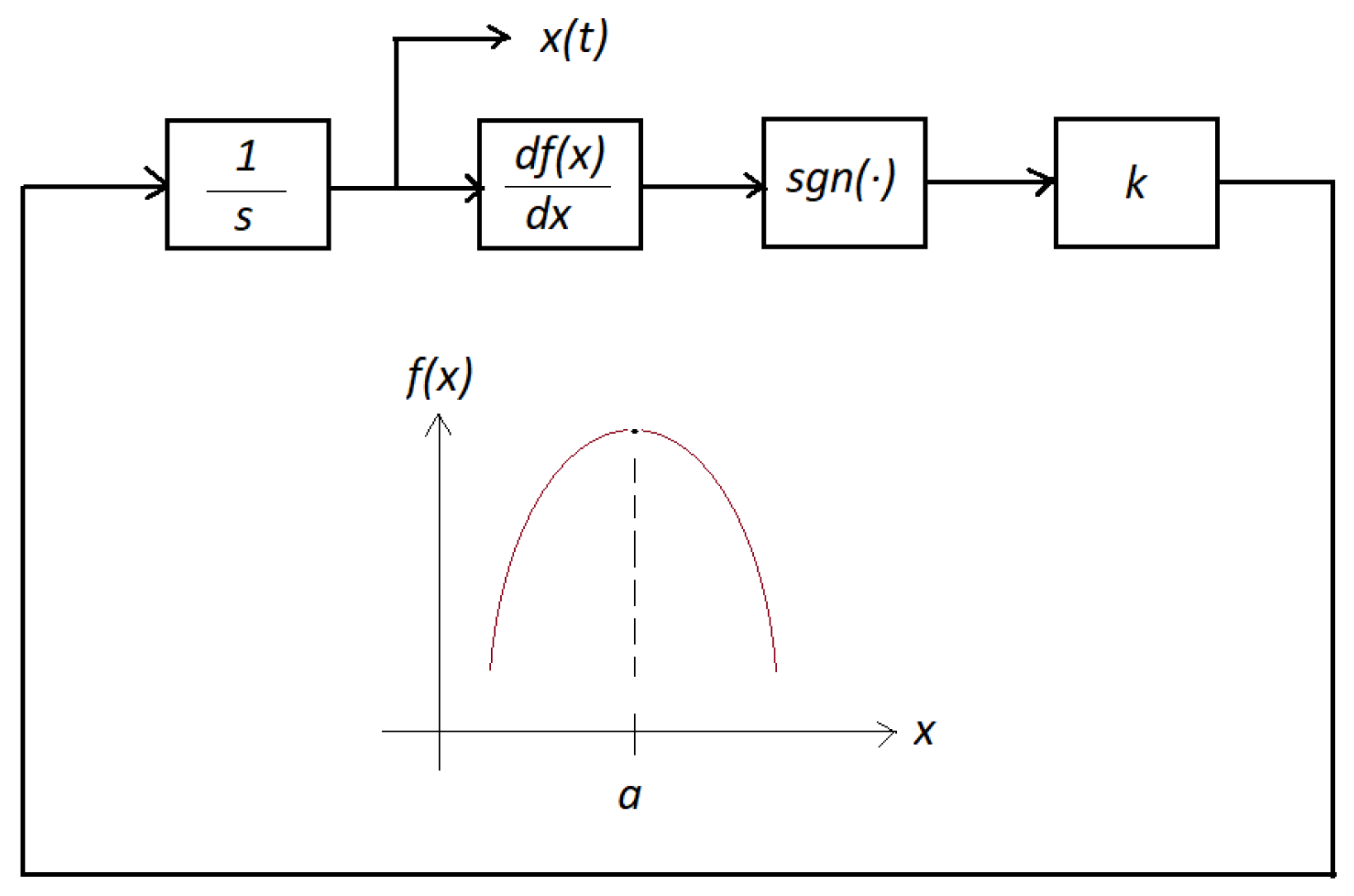
(Dynamical optimizer). Given a smooth concave function with a single maximum point at , and k being a given positive constant value, the dynamic optimizer given in Figure 1 produces a finite-time convergence of to a. That is, there exists value , such that:
Proof.
See [8]. □
Obviously, the following assumptions are inherent:
- There is only one maximum point of the function.
- The function is concave.
Moreover, the parameter k controls the speed of convergence of the optimizer output response. Finally, a numerical example is shown in Figure 2 with , where the extremum of the function is located at .
3. The Recent Control Scheme
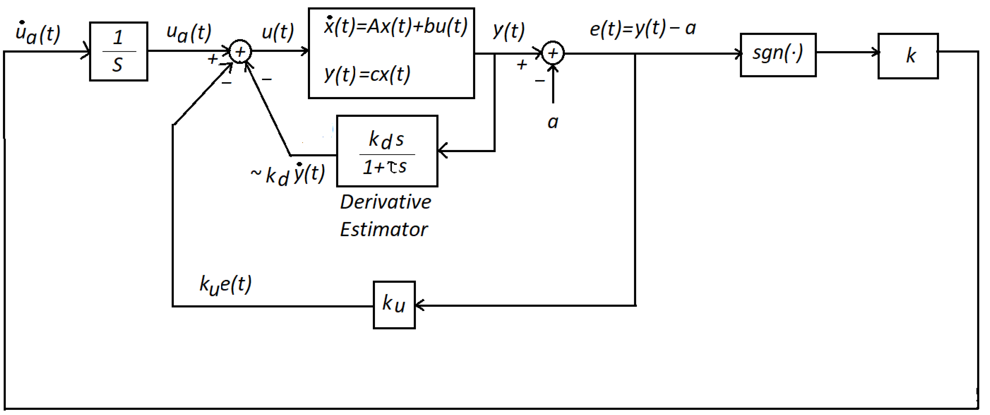
The main objective of this section is to introduce our new approach to the regulation control statement using our dynamic optimizer, as seen in Figure 3. Finite-time convergence was also a goal. We considered the system to be stabilized was linear with an input and an output, and of a second order, given by:
where is the state vector of the system, and and are the input and output of the system, respectively. Additionally, the proposed model (2) and (3) is expressed in its canonical format:
and
Therefore, , , and are the system parameters, and all are assumed to be constant values. On the other hand, we considered that the performance index was, instead, a convex function, and given by . The parameter a was a given constant value. Hence, , as seen in Figure 3.
Next, is our main result.
Theorem 2
(Control scheme). The closed-loop system, shown in Figure 3, was globally-stable having finite-time convergence of to a bounded set. That is, there existed a constant , such that:
where , and is a constant value representing the reference command signal, if the following conditions are satisfied:
- There is a real constant value such that , with ,
- There is a real constant value such that , with ,
- There is a real constant value k such that , with .
The next closed-loop system parameters setting was as follows:
- The parameter was sufficiently large with respect to (),
- The relation was sufficiently small ().
Proof.
From the block diagram shown in Figure 3, we could obtain:
Its time derivative, using the system model (2) and (3), yielded:
Once again, the time derivative of the above equation, using the system data (2) and (3), resulted in:
From Figure 3, we obtained:
Next, by taking into account that , , and , the equations are reduced to:
Thereupon, if:
- ; ,
- ; ,
then Equation (12) gives:
In the next place, the time-derivative of (13) shows:
Later on, taking into account that , we have:
Let us define:
Then, the system (15) yields:
Double time integration of (17) results in:
Now, if is large enough, the system (18) has a fast dynamic converging to:
where , the slow dynamic, is the solution to (16) by using (18) and (19):
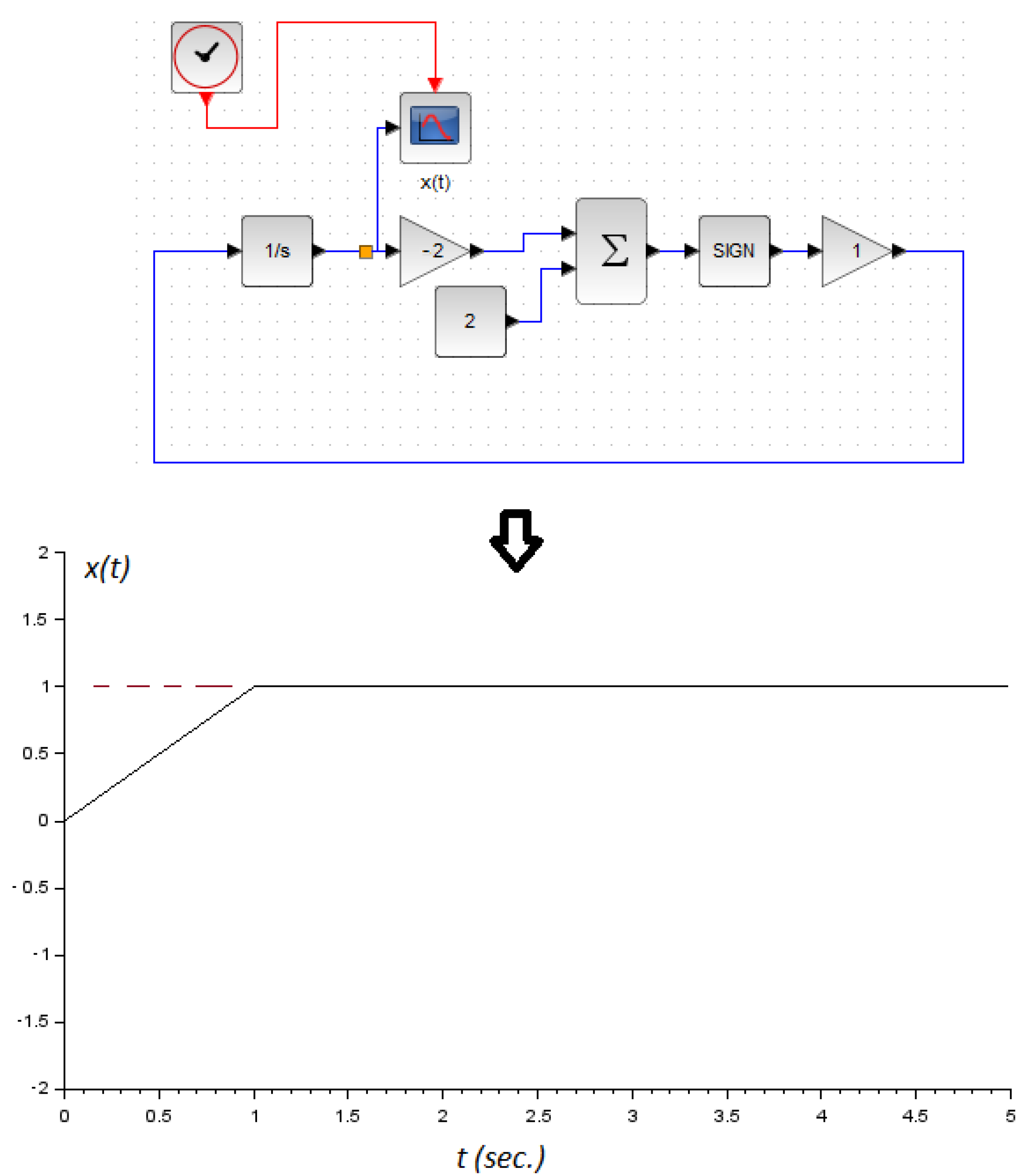
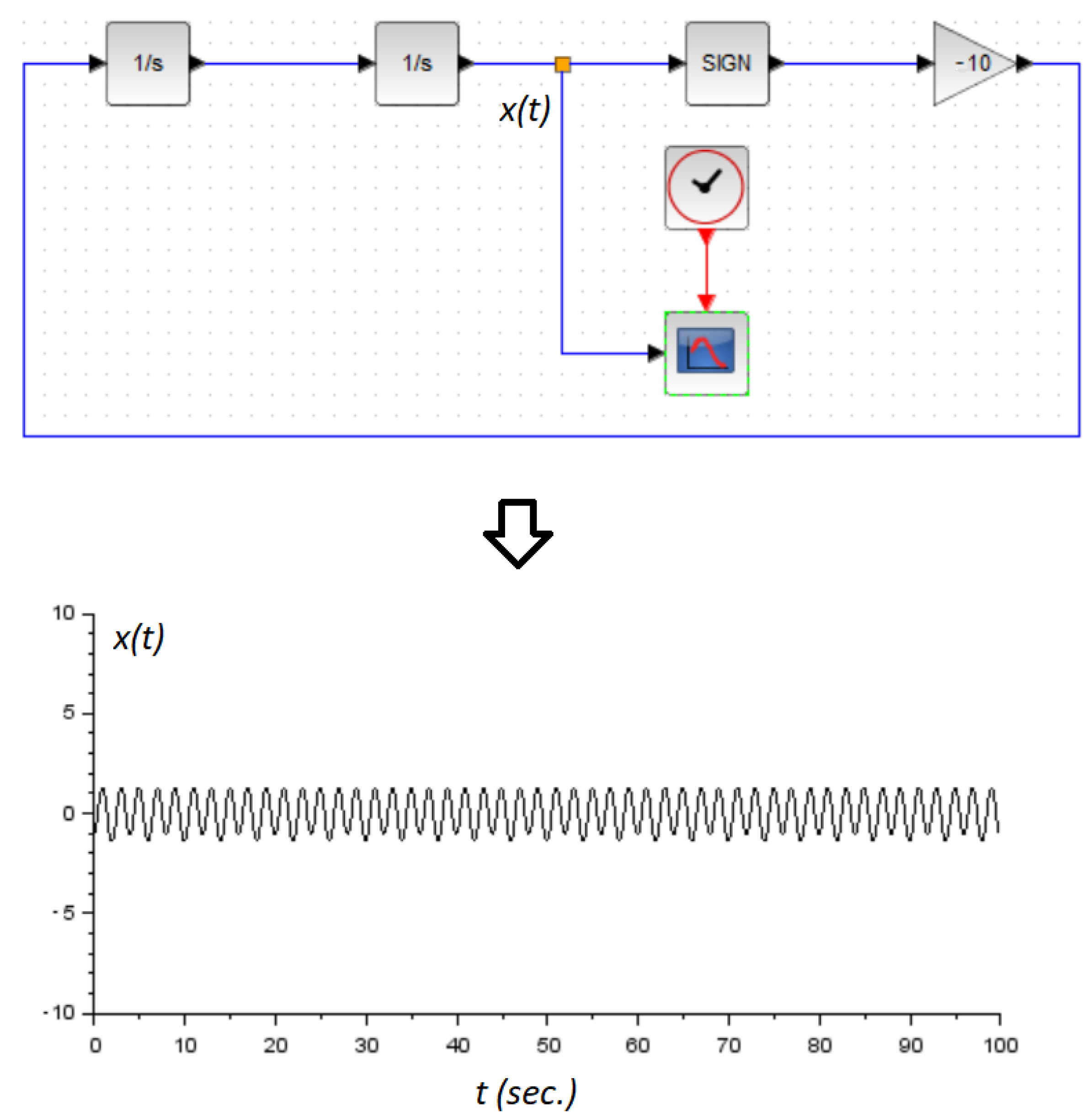
System (20) represents a stable oscillator (See chapter 2 in [26]) with its amplitude proportional to the initial conditions of the system, and its oscillating frequency related to . A numerical example is displayed in Figure 4 with . The stability of this system (20) can be verified by invoking the next Lyapunov function:
where its time derivative along the system trajectory (20) yields:
implying stability of the cited system. This also concludes that all signals in the closed-loop system are bounded. Finite-time stability is assured, due to the convergence of the closed-loop system to its internal oscillator dynamic, and related to (19). □
Regarding proof development, it was assumed that the signum function is given by:
To give numerical examples, let us use the following system related to (2) and (3):
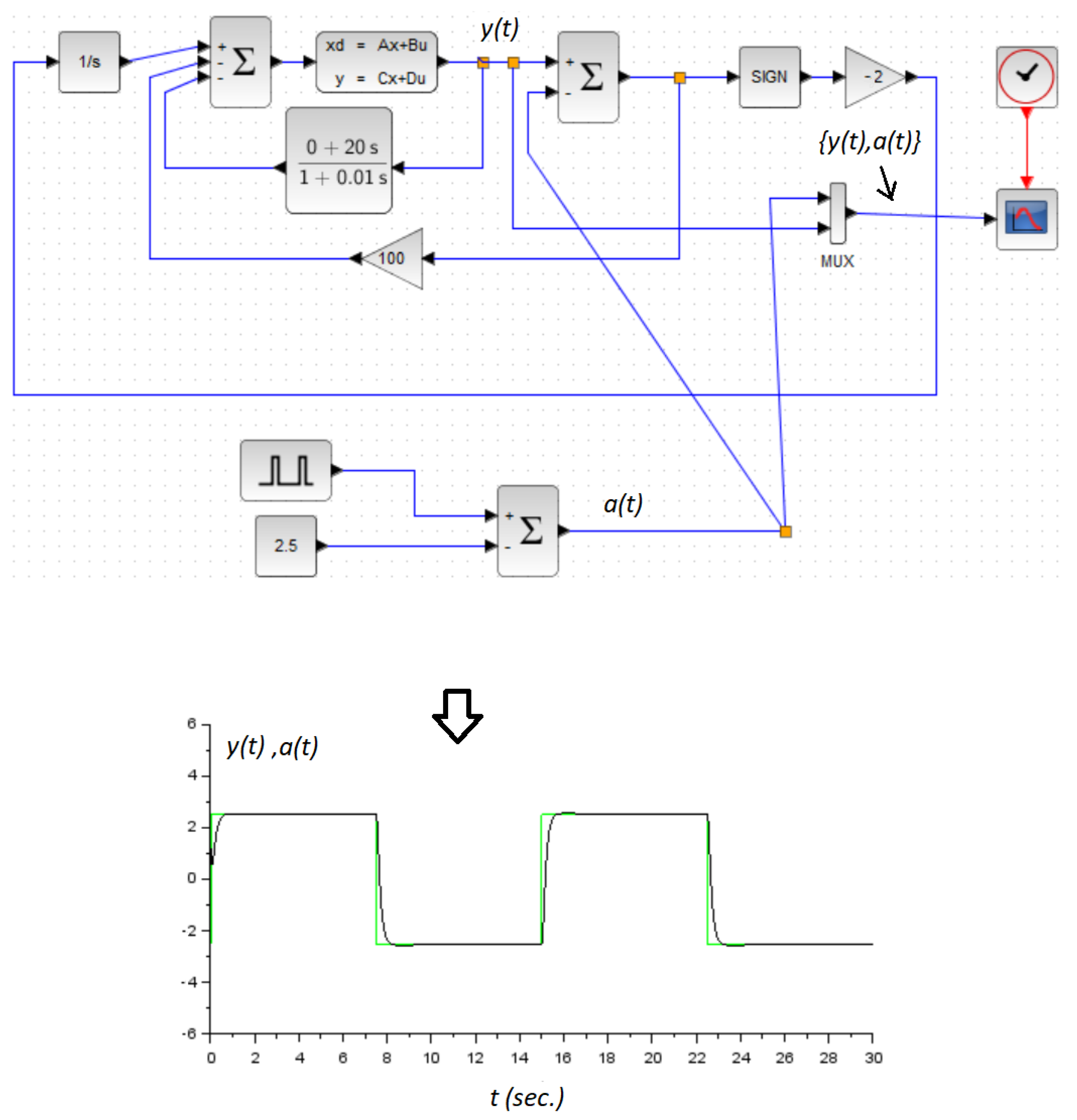
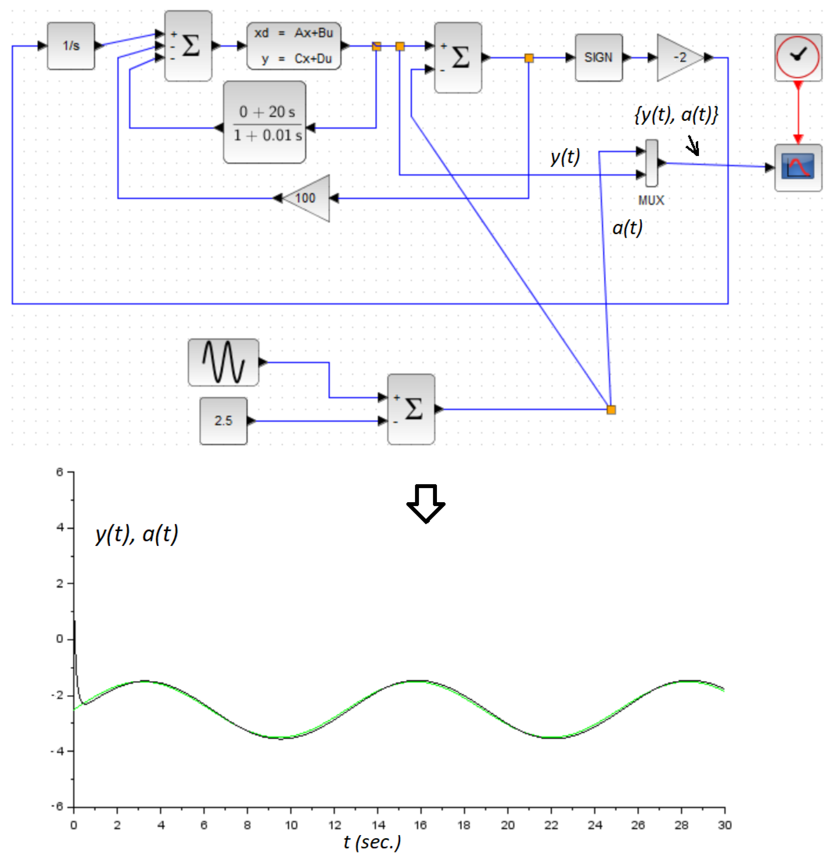
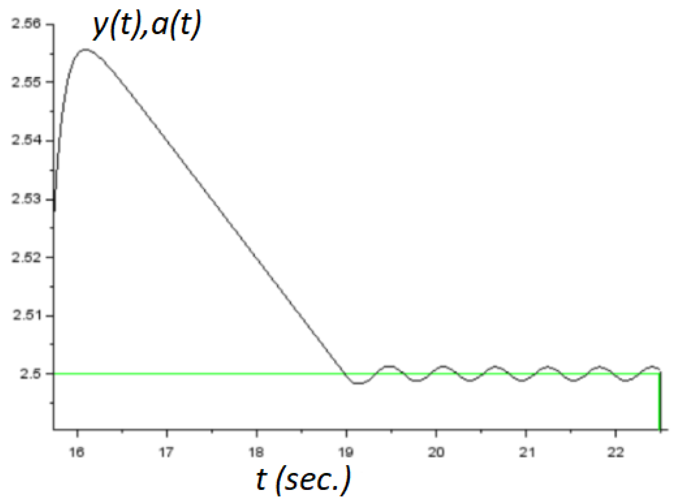
It was clear that this system was unstable. It could be verified that the conditions demanded by Theorem 2 were satisfied with , , and . On the other hand, in the derivative estimator, we set the time-constant . Figure 5 and Figure 6 showed the obtained numerical results. In both numerical experiments, the initial conditions were and . The simulations were carried out using the application from the open source platform. Additionally, in this application, we used the integration method called . Obviously, the parameter a was used here as the command signal. It was assumed constant for control design only, and we demonstrated the performance of the controller by allowing it to be a time-varying signal. Additionally, a zoom in version of the Figure 5 is shown in Figure 7.
4. Application to a Micromachine Device
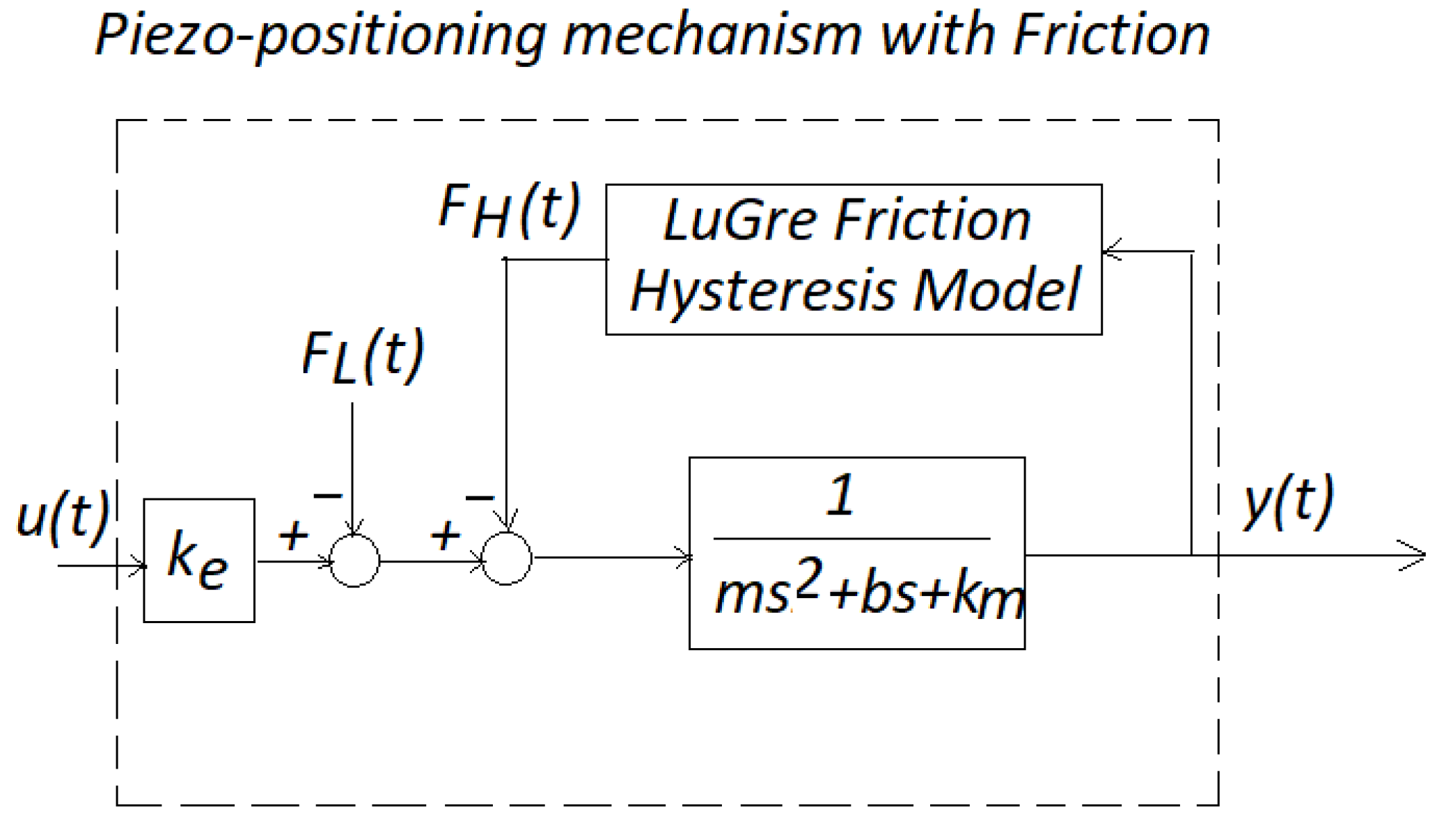
A schematic model of a piezoelectric positioning mechanism with friction is shown in Figure 8, where Kg, Ns/m, and N/m. See details in [1]. With these data, the system had the following information related to (2) and (3):
Additionally, the LuGre friction model (see Figure 8), was experimentally verified in [1], given by
and
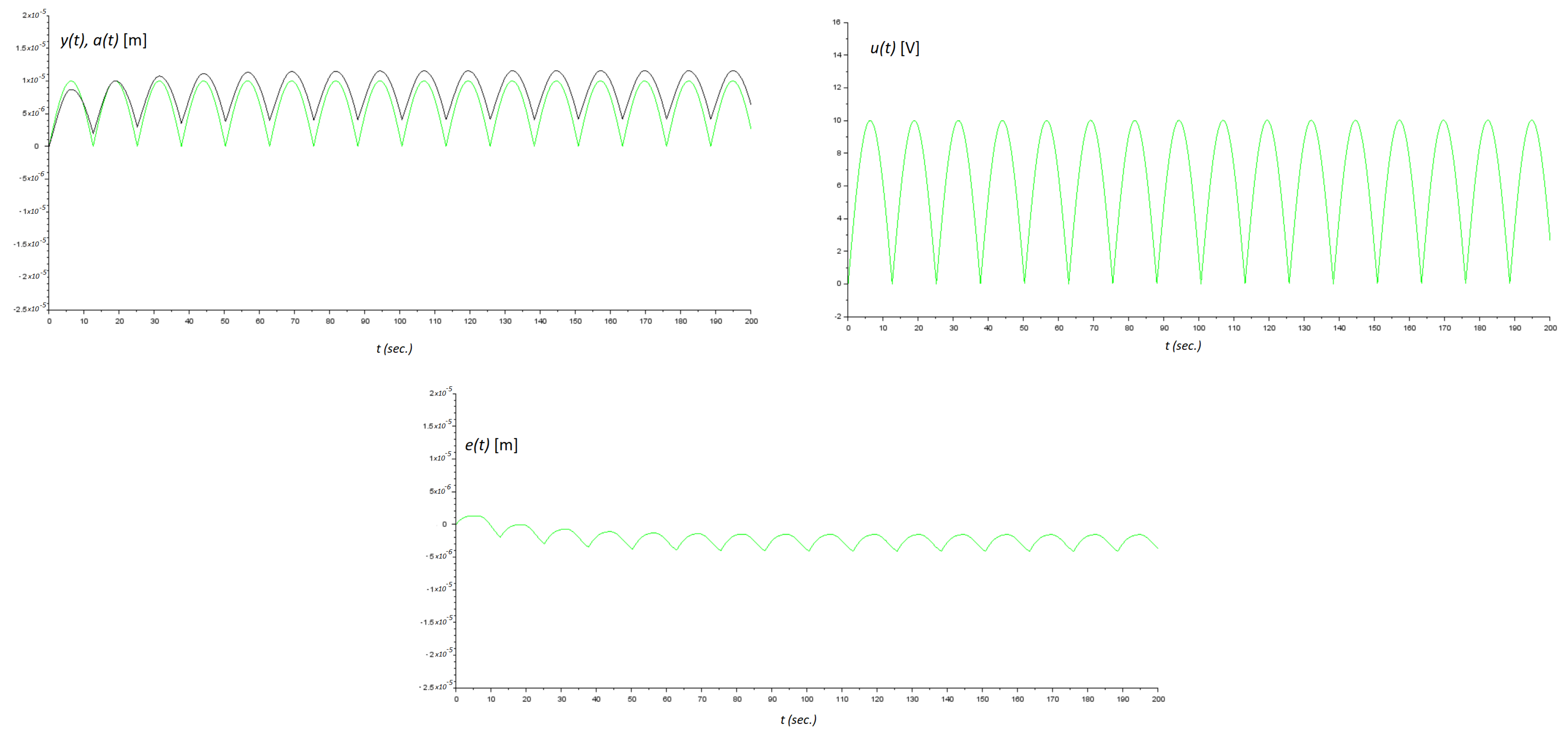
On the other hand, represented load variations and uncertainties due to modeling and external perturbations [1]. Here, in realizing our friction model, we used the estimation of the velocity information of the mechanism. Therefore, there existed model uncertainty, such that was indirectly induced in our numerical experimentation. was the gain converting the applied voltage to the piezo-positioning micromachine to Newton force. Figure 9 shows the implementation of our controller for this friction micromachine using , as was previously invoked. Zero initial conditions on the plant was realized. Figure 10 shows the numerical experimental results. In Figure 9, notice that we used a gain block of to scale for the readout. This same gain block for data acquisition is also called in [3]. Finally, to measure the performance of the control action, we performed the following time-error calculation in s:
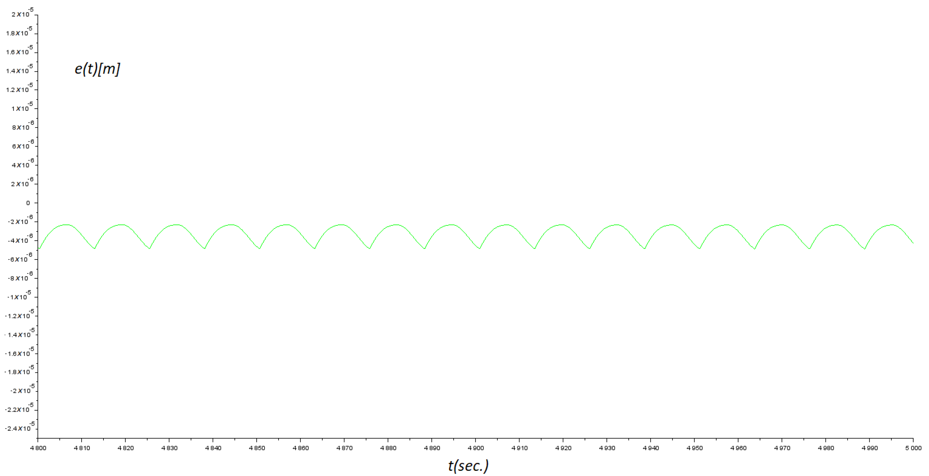
yielding μm. Obviously, this value was in the micros-scale of micromachine devices. The maximum absolute error in the steady-state response was μm. Compared to [1], the maximum absolute error obtained was approximately μm for the tracking control case. Additionally, the control parameter affected the damping closed-loop dynamic behaviour, and k regulated the amplitude and the settling-time of the oscillating steady-state error signal. See Table 2 for a particular discussion. Finally, Figure 11 shows the final part of a long-term simulation.
Some additional comments. Mathematical modeling of piezo-positioning micromachines is not unique. First, because there are many friction models [7]. Second, the parametric identification is not unique for a given system [2]. Finally, a tracking error is observed in our numerical experiments, as well as in [3].
5. Future Work
Our control approach was based on the self-generation of a high frequency signal of small amplitude but without chattering. For some time, designing a sliding mode controller without chattering has been, amd still is, an important issue [27,28,29]. Our control scheme can be classified as a switching controller, because of the signum function where chattering is absent. Therefore, one option to improve our control performance is to incorporate more complex switching signals, as evidenced, for instance, in [30]. On the other hand, our control method implicitly generates the dynamics of an oscillator but its amplitude depends on its initial conditions. However, another option is to use an oscillating system with an asymptotically stable limit cycle, for example, as the one shown in [31,32]. Finally, another way to improve control performance is to add a friction compensator to the control law [33,34,35].
As future work, we aime to develop our control scheme by means of low cost electronics. This is because our control scheme can be fully assembled using only operational amplifiers (op-amps). Even the derivative estimator block in Figure 3 can be realized using op-amps. Op-amps are low-cost electronic units. Therefore, we have in mind to do this in our laboratory.
6. Conclusions
Based on a dynamic optimizer scheme with finite-time stability, a recent control approach was developed. In this approach, a self-oscillating signal was generated to meet the control statement objective. The control structure obtained seemed simple, and was even achievable through the use of analog electronics, such as operational amplifiers. In addition, the stability of the closed-loop system followed a recent point of view. Finally, controller performance was numerically evaluated by using a realistic LuGre friction model for micromachines.
Funding
This research received no external funding.
Data Availability Statement
Data sharing not applicable.
Conflicts of Interest
The author declares no conflict of interest.
References
- Wang, G.; Xu, Q. LuGre model based hysteresis compensation of a piezo-actuated mechanism. In Proceedings of the International Conference on Intelligent Autonomous Systems, Shanghai, China, 3–7 July 2016; pp. 645–657. [Google Scholar]
- Liu, Y.T.; Chang, K.M.; Li, W.Z. Model reference adaptive control for a piezo-positioning system. Precis. Eng. 2010, 34, 62–69. [Google Scholar] [CrossRef]
- Lin, J.; Chiang, H.; Lin, C. Tuning PID control parameters for micro-piezo-stage by using grey relational analysis. Expert Syst. Appl. 2011, 38, 13924–13932. [Google Scholar] [CrossRef]
- Edeler, C.; Meyer, I.; Fatikow, S. Modeling of stick-slip micro-drives. J. Micro-Nano Mechatron. 2011, 6, 65–87. [Google Scholar] [CrossRef]
- Ounissi, A.; Yakoub, K.; Kaddouri, A.; Abdessemed, R. Robust adaptive displacement tracking control of a piezo-actuated stage. In Proceedings of the 2017 6th International Conference on Systems and Control (ICSC), Batna, Algeria, 7–9 May 2017; pp. 297–302. [Google Scholar]
- Fan, S.X.; Fan, D.P.; Hong, H.J.; Zhang, Z.Y. Robust tracking control for micro machine tools with load uncertainties. J. Cent. South Univ. 2012, 19, 117–127. [Google Scholar] [CrossRef]
- Dinh, T.X.; Ahn, K.K. Radial basis function neural network based adaptive fast nonsingular terminal sliding mode controller for piezo positioning stage. Int. J. Control Autom. Syst. 2017, 15, 2892–2905. [Google Scholar] [CrossRef]
- Acho, L. An educational example to the maximum power transfer objective in electric circuits using a PD-controlled DC—Driver. IFAC-PapersOnLine 2016, 49, 344–347. [Google Scholar] [CrossRef]
- Bryson, A.E. Optimal control-1950 to 1985. IEEE Control Syst. Mag. 1996, 16, 26–33. [Google Scholar] [CrossRef]
- Polak, E. An historical survey of computational methods in optimal control. SIAM Rev. 1973, 15, 553–584. [Google Scholar] [CrossRef]
- Zhang, Y.; Li, S.; Liao, L. Near-optimal control of nonlinear dynamical systems: A brief survey. Annu. Rev. Control 2019, 47, 71–80. [Google Scholar] [CrossRef]
- Nešić, D. Extremum seeking control: Convergence analysis. Eur. J. Control 2009, 15, 331–347. [Google Scholar] [CrossRef]
- Salsbury, T.I.; House, J.M.; Alcala, C.F. Self-perturbing extremum-seeking controller with adaptive gain. Control Eng. Pract. 2020, 101, 104456. [Google Scholar] [CrossRef]
- Torres-Zúñiga, I.; Lopez-Caamal, F.; Hernandez-Escoto, H.; Alcaraz-Gonzalez, V. Extremum seeking control and gradient estimation based on the Super-Twisting algorithm. J. Process Control 2021, 105, 223–235. [Google Scholar] [CrossRef]
- Zhang, C.; Ordóñez, R. Extremum-Seeking Control and Applications: A Numerical Optimization-Based Approach; Springer Science & Business Media: Berlin/Heidelberg, Germany, 2011. [Google Scholar]
- Scheinker, A.; Krstić, M. Model-Free Stabilization by Extremum Seeking; Springer: Berlin/Heidelberg, Germany, 2017. [Google Scholar]
- Tan, Y.; Moase, W.H.; Manzie, C.; Nešić, D.; Mareels, I.M. Extremum seeking from 1922 to 2010. In Proceedings of the 29th Chinese Control Conference, Beijing, China, 29–31 July 2010; pp. 14–26. [Google Scholar]
- Kim, D.; Cha, K.; Sung, I.; Bryan, J. Design of surface micro-structures for friction control in micro-systems applications. CIRP Ann. 2002, 51, 495–498. [Google Scholar] [CrossRef]
- Lumbantobing, A.; Komvopoulos, K. Static friction in polysilicon surface micromachines. J. Microelectromech. Syst. 2005, 14, 651–663. [Google Scholar] [CrossRef]
- Xiang, H.; Komvopoulos, K. Effect of fluorocarbon self-assembled monolayer films on sidewall adhesion and friction of surface micromachines with impacting and sliding contact interfaces. J. Appl. Phys. 2013, 113, 224505. [Google Scholar] [CrossRef]
- Shroff, S.S.; de Boer, M.P. Full Assessment of Micromachine Friction Within the Rate–State Framework: Experiments. Tribol. Lett. 2016, 63, 1–15. [Google Scholar] [CrossRef]
- Shroff, S.S.; de Boer, M.P. Direct observation of the velocity contribution to friction in monolayer-coated micromachines. Extrem. Mech. Lett. 2016, 8, 184–190. [Google Scholar] [CrossRef]
- Lu, Y.; Lu, J.; Tan, C.; Tian, M.; Dong, G. Adaptive Non-Singular Terminal Sliding Mode Control Method for Electromagnetic Linear Actuator. Micromachines 2022, 13, 1294. [Google Scholar] [CrossRef]
- Dumanli, A.; Sencer, B. Pre-compensation of servo tracking errors through data-based reference trajectory modification. CIRP Ann. 2019, 68, 397–400. [Google Scholar] [CrossRef]
- Khalil, H. Nonlinear Systems; Pearson Education, Prentice Hall: Englewood Cliffs, NJ, USA, 2002. [Google Scholar]
- Slotine, J.J.E.; Li, W. Applied Nonlinear Control; Prentice Hall: Englewood Cliffs, NJ, USA, 1991; Volume 199. [Google Scholar]
- Ho, H.; Wong, Y.K.; Rad, A.B. Adaptive fuzzy sliding mode control with chattering elimination for nonlinear SISO systems. Simul. Model. Pract. Theory 2009, 17, 1199–1210. [Google Scholar] [CrossRef]
- Bartolini, G.; Punta, E. Chattering elimination with second-order sliding modes robust to coulomb friction. J. Dyn. Syst. Meas. Control 2000, 122, 679–686. [Google Scholar] [CrossRef]
- Al-Hadithi, B.M.; Barragan, A.J.; Andújar, J.M.; Jimenez, A. Variable Structure Control with chattering elimination and guaranteed stability for a generalized TS model. Appl. Soft Comput. 2013, 13, 4802–4812. [Google Scholar] [CrossRef]
- Levant, A. Homogeneity approach to high-order sliding mode design. Automatica 2005, 41, 823–830. [Google Scholar] [CrossRef]
- Orlov, Y.; Aguilar, L.T.; Acho, L.; Ortiz, A. Asymptotic harmonic generator and its application to finite time orbital stabilization of a friction pendulum with experimental verification. Int. J. Control 2008, 81, 227–234. [Google Scholar] [CrossRef]
- Shtessel, Y.; Kaveh, P.; Ashrafi, A. Harmonic oscillator utilizing double-fold integral, traditional and second-order sliding mode control. J. Frankl. Inst. 2009, 346, 872–888. [Google Scholar] [CrossRef]
- Olsson, H.; Åström, K.J.; De Wit, C.C.; Gäfvert, M.; Lischinsky, P. Friction models and friction compensation. Eur. J. Control 1998, 4, 176–195. [Google Scholar] [CrossRef]
- Guerra, R.; Acho, L.; Aguilar, L. Adaptive friction compensation for mechanisms: A new perspective. Int. J. Robot. Autom. 2007, 22, 155–159. [Google Scholar] [CrossRef]
- Guerra, R.; Acho, L. Adaptive friction compensation for tracking control of mechanisms. Asian J. Control 2007, 9, 422–425. [Google Scholar] [CrossRef]
Figure 1.
Dynamical optimizer.

Figure 2.
A numerical example using from application, where the numerical integration method used was . The concave function is . Note that the notation for the signum function in the environment is .
Figure 2.
A numerical example using from application, where the numerical integration method used was . The concave function is . Note that the notation for the signum function in the environment is .

Figure 3.
A recent control scheme using a dynamic optimizer. The parameter in the derivative estimator block was assumed to be small. This is a well-known derivative block (see, for instance, reference [25], p. 495).
Figure 3.
A recent control scheme using a dynamic optimizer. The parameter in the derivative estimator block was assumed to be small. This is a well-known derivative block (see, for instance, reference [25], p. 495).

Figure 4.
Numerical example of the oscillator dynamic (20). (Top): the Xcos block diagram of the system. (Bottom): the system response versus time. We use and .
Figure 4.
Numerical example of the oscillator dynamic (20). (Top): the Xcos block diagram of the system. (Bottom): the system response versus time. We use and .

Figure 5.
Numerical example: A pulse reference signal case. The green line is the reference signal , and the black line is the system response .
Figure 5.
Numerical example: A pulse reference signal case. The green line is the reference signal , and the black line is the system response .

Figure 6.
Numerical example: A sinusoidal reference signal case. The green line is the reference signal , and the black line is the system response .
Figure 6.
Numerical example: A sinusoidal reference signal case. The green line is the reference signal , and the black line is the system response .

Figure 7.
An enlarged view of the Figure 5.
Figure 7.
An enlarged view of the Figure 5.

Figure 8.
Model of a piezo-positioning mechanism with friction.

Figure 9.
A control scheme for the positioning micromachine system using .

Figure 10.
Results of numerical experiments. Top left: the green line is the reference signal and the black line is the position response of the micromachine . Top right: control signal . At the bottom: Error signal between system output and reference command .
Figure 10.
Results of numerical experiments. Top left: the green line is the reference signal and the black line is the position response of the micromachine . Top right: control signal . At the bottom: Error signal between system output and reference command .

Figure 11.
Results of numerical experiments. Error signal between system output and reference command . The final part of a long-term simulation.
Figure 11.
Results of numerical experiments. Error signal between system output and reference command . The final part of a long-term simulation.


Table 1.
Main challenges for control design.
| Challenge | Strategy | Evidence |
|---|---|---|
| Incorporate a dynamic optimizer in a closed-loop system | Search for a structure where the control signal is integrated to reduce the vibration that the optimizer and the plant could produce | Through numerical experiments |
| Closed-loop stability test | Invoke the theory of stability in the sense of Lyapunov | Verifying that the conditions of Lyapunov’s theory are met |
| To test control performance in a frictional micromachine using an experimentally validated system model | Use of numerical experiments | From numerical data, observe acceptable performance |
Table 2.
Effects of the controller parameters on the dynamics of the closed-loop system (data obtained from numerical experimentation by independently increasing each control parameter).
Table 2.
Effects of the controller parameters on the dynamics of the closed-loop system (data obtained from numerical experimentation by independently increasing each control parameter).
| Control Parameter | Steady-State Error | Transient Time Duration |
|---|---|---|
| k | – | ↓ |
| ↑ | ↓ | |
| ↑ | – |
Disclaimer/Publisher’s Note: The statements, opinions and data contained in all publications are solely those of the individual author(s) and contributor(s) and not of MDPI and/or the editor(s). MDPI and/or the editor(s) disclaim responsibility for any injury to people or property resulting from any ideas, methods, instructions or products referred to in the content. |
© 2023 by the author. Licensee MDPI, Basel, Switzerland. This article is an open access article distributed under the terms and conditions of the Creative Commons Attribution (CC BY) license (https://creativecommons.org/licenses/by/4.0/).
Share and Cite
MDPI and ACS Style
Acho, L. A Control Method Based on a Simple Dynamic Optimizer: An Application to Micromachines with Friction. Micromachines 2023, 14, 387. https://doi.org/10.3390/mi14020387
AMA Style
Acho L. A Control Method Based on a Simple Dynamic Optimizer: An Application to Micromachines with Friction. Micromachines. 2023; 14(2):387. https://doi.org/10.3390/mi14020387
Chicago/Turabian StyleAcho, Leonardo. 2023. "A Control Method Based on a Simple Dynamic Optimizer: An Application to Micromachines with Friction" Micromachines 14, no. 2: 387. https://doi.org/10.3390/mi14020387
Note that from the first issue of 2016, this journal uses article numbers instead of page numbers. See further details here.