Article

A Space Target Detection Method Based on Spatial–Temporal Local Registration in Complicated Backgrounds

1
Shanghai Institute of Technical Physics, Chinese Academy of Sciences, Shanghai 200083, China
2
Key Laboratory of Intelligent Infrared Perception, Chinese Academy of Sciences, Shanghai 200083, China
3
University of Chinese Academy of Sciences, Beijing 100049, China
*
Author to whom correspondence should be addressed.
Remote Sens. 2024, 16(4), 669; https://doi.org/10.3390/rs16040669
Submission received: 7 January 2024 / Revised: 7 February 2024 / Accepted: 8 February 2024 / Published: 13 February 2024
(This article belongs to the Special Issue Laser and Optical Remote Sensing for Planetary Exploration)

Abstract

:
Human space exploration has brought a growing crowded operating environment for in-orbit spacecraft. Monitoring the space environment and detecting space targets with photoelectric equipment has extensive and realistic significance in space safety. In this study, a local spatial–temporal registration (LSTR) method is proposed to detect moving small targets in space. Firstly, we applied the local region registration to estimate the neighbor background motion model. Secondly, we analyzed the temporal local grayscale difference between the strong clutter and target region and measured the temporal local–central region difference to enhance the target. Then, the temporal pixel contrast map was calculated, which further retains the target signal and suppresses the residue clutter. Finally, a simple adaptive threshold segmentation algorithm was applied to the saliency map to segment the targets. Comparative experiments were conducted on four groups of image sequences to validate the efficiency and robustness of the algorithm. The experimental findings indicate that the proposed method performs well in target enhancement and clutter suppression under different scenarios.

1. Introduction

1.1. Background

Space targets refer to all objects in outer space, including space debris, spacecraft, meteorites, and comets. With the deepening of space exploration, the increasing number of space targets is bringing an ongoing crowded space environment and interfering with space exploration tasks [1]. Space situational awareness (SSA) refers to observing, understanding, and predicting the physical location of organic and artificial objects in orbit around the Earth [2]. Investigating the detection and tracking of space targets using image data surrounding spacecraft acquired from space-based optical detection equipment is beneficial to advancing SSA technology and ensuring space environment safety [3,4].
As the main task of SSA, spaceborne space-target-monitoring technology has received much attention. Under the space-based monitoring scenario, it is common to use wide-field view optical detection equipment to obtain comprehensive space environment information [5]. Moreover, the space target appears as a dim point in the image due to the long distance between the target and the focal plane of photoelectric equipment [6]. Most previous research efforts have concentrated on space-based space target detection in deep-space backgrounds [7]. These studies have been dedicated to addressing various challenges, including star map matching [8], stellar target suppression [9], and the enhancement of low signal-to-noise ratio space targets [10]. However, the clutter interference derived from the ground surface, moving clouds, and atmospheric turbulence will invariably enter the field of view, increasing the complexity of the space target image background and the difficulty of target detection. Therefore, this work aims to provide a reliable moving-space-target detection algorithm under a complex background that can achieve the accurate detection of weak and small space targets under the space-based monitoring scenario.

1.2. Motivation

The challenges of space moving-target detection in the complex space-based background can be summarized as the following two points: Firstly, with a broad detection range, the distance between the target and the imaging plane may reach hundreds of kilometers. The detection distance and the target size often lead to a reduction in the pixel number and a relatively weak grayscale response of the space target on the image. It means that the detector fails to use the morphological information of the target with a limited number of pixels, leading to primary demands for optimizing the target enhancement capability of the detector. Secondly, the clutter interference derived from the ground surface, moving clouds, and atmospheric turbulence will invariably enter the field of view, increasing the complexity of the space target image background. Strong background clutter is often imaged in blocks or dots with a high grayscale intensity on the focal plane. In particular, the distribution pattern of point clutter may be similar to the target, affecting the detection accuracy. Strong non-stationary background interferences must be rejected to obtain better detection and false alarm rates.
Some existing dim and weak target detection algorithms are often applied to the ground scene with a simple and stable background. The existing detection methods that utilize spatial and temporal grayscale feature information can effectively detect targets in simple backgrounds of sequence images. However, they fail to extract targets accurately when the image background changes under space-based platforms. There is still limited research on space target detection algorithms in the space-based scenario.
In this study, we propose a local spatial–temporal registration (LSTR) method to enhance weak targets and alleviate background interference for the space moving-target detection of sequence images. This method is suitable for small-moving-target detection under space-based complicated scenes. Specifically, the contributions of the proposed LSTR method are mainly in four aspects:
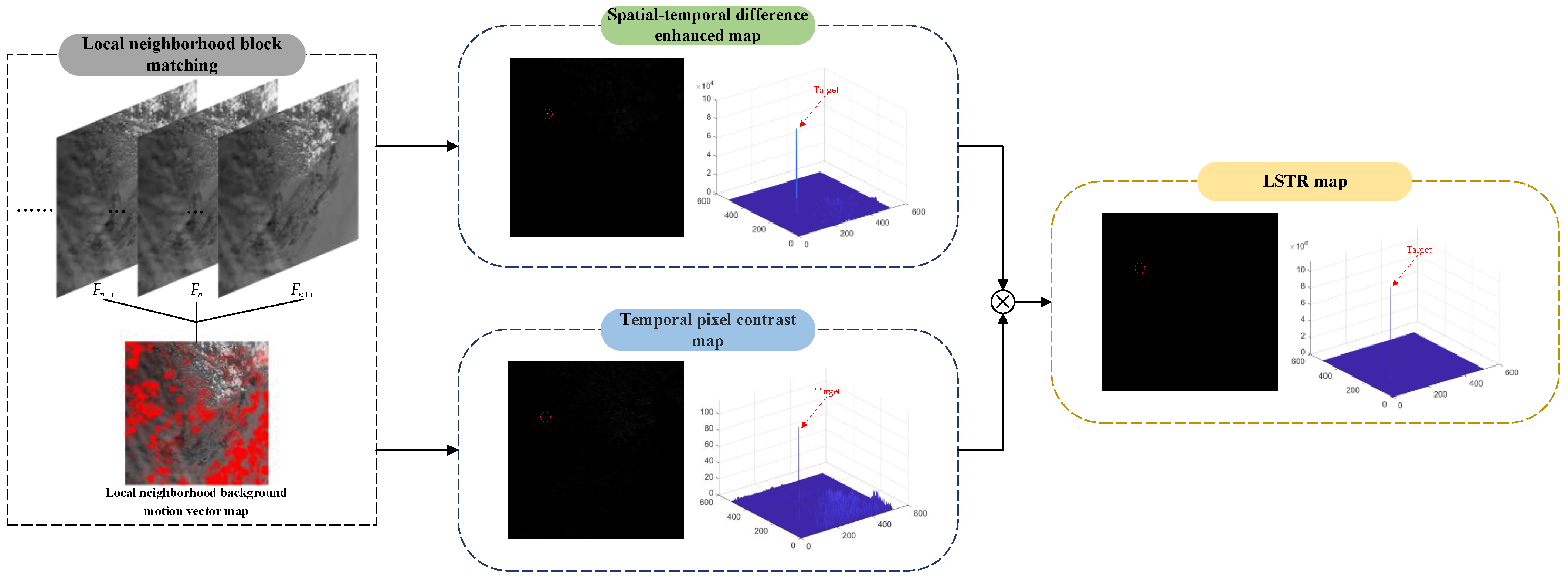
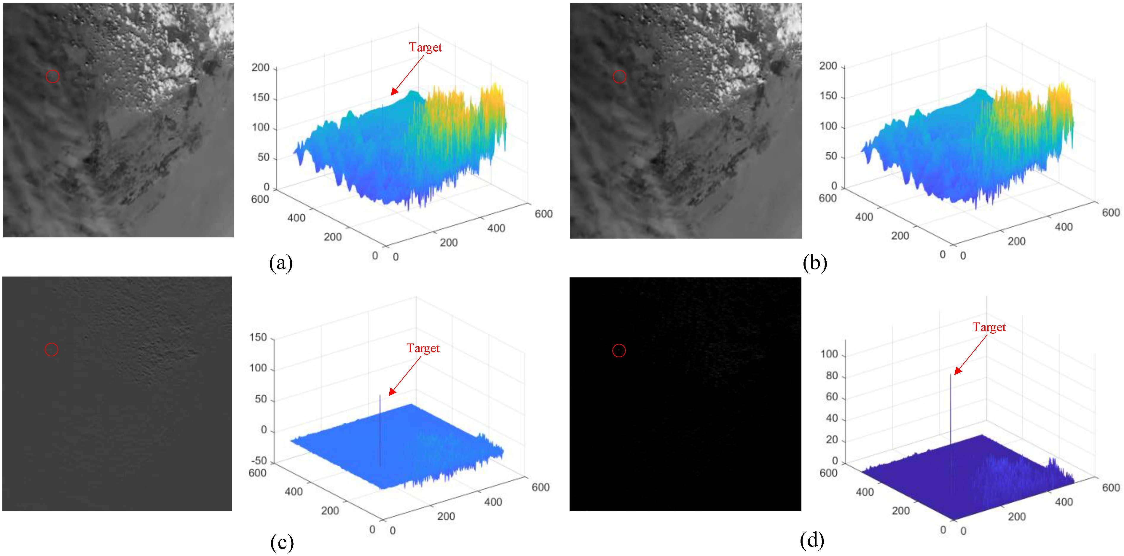
  • A method for space moving-target detection under complex backgrounds is proposed. It uses the motion difference between the target and its local surrounding background region to highlight the target and reduce strong background clutter. A spatial–temporal difference enhancement map and A temporal pixel contrast map are calculated to enhance the target signal.
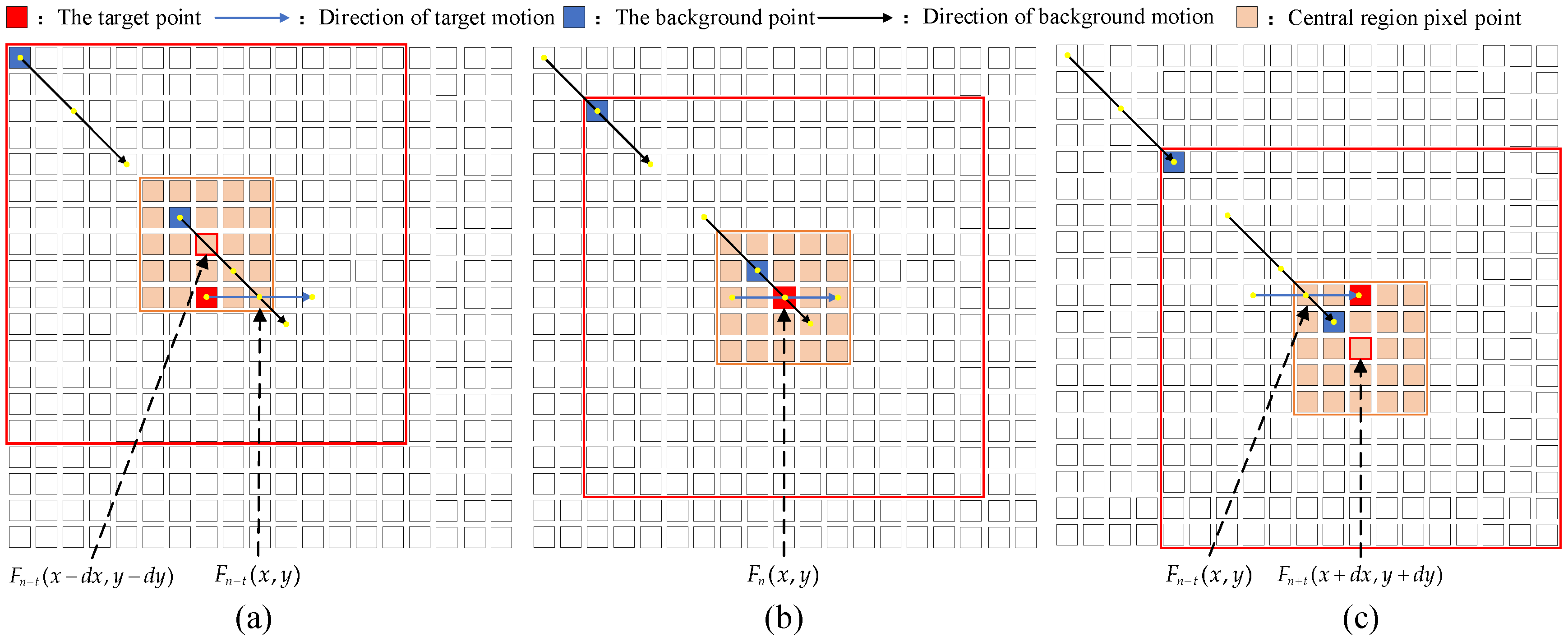
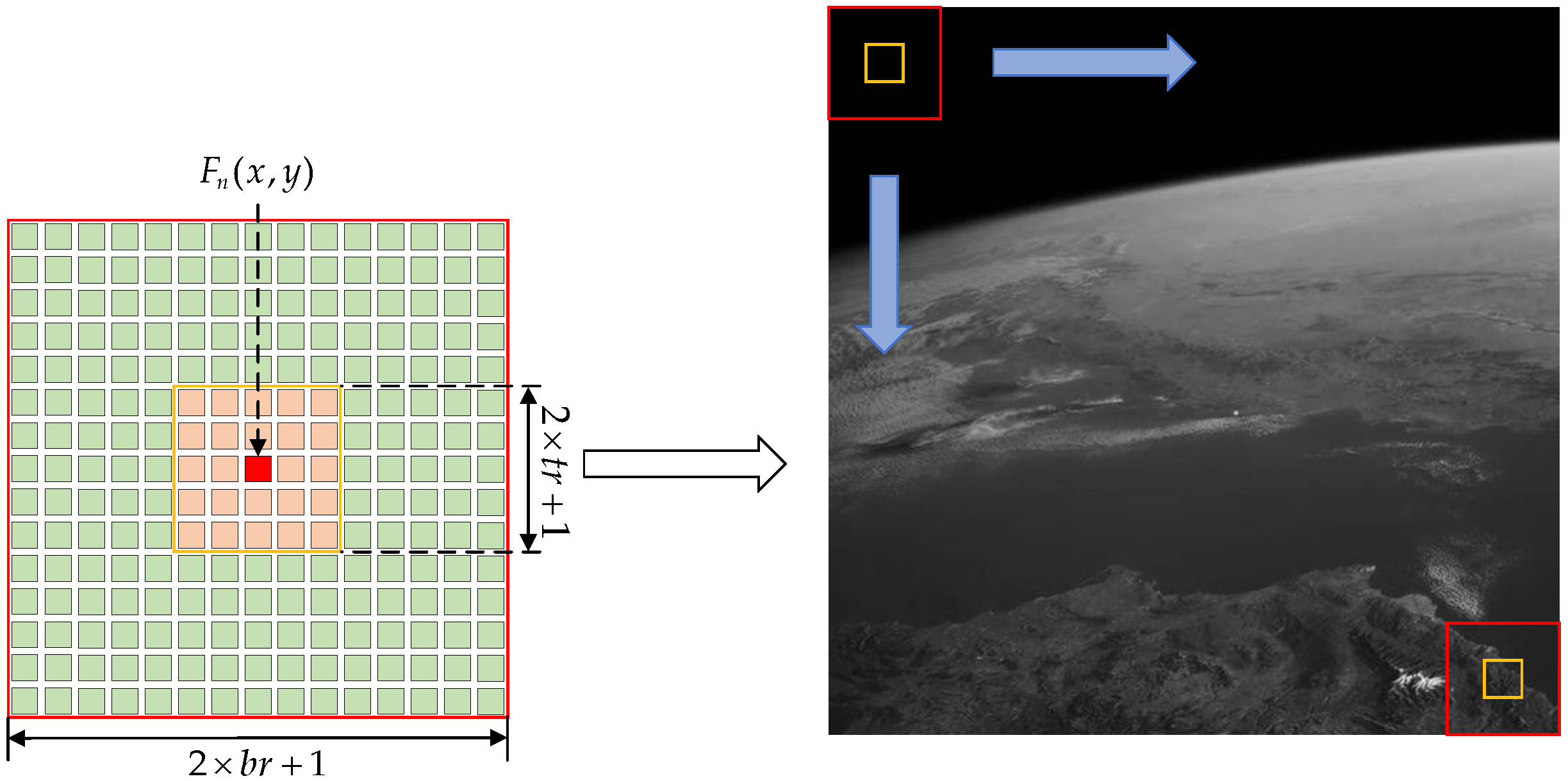
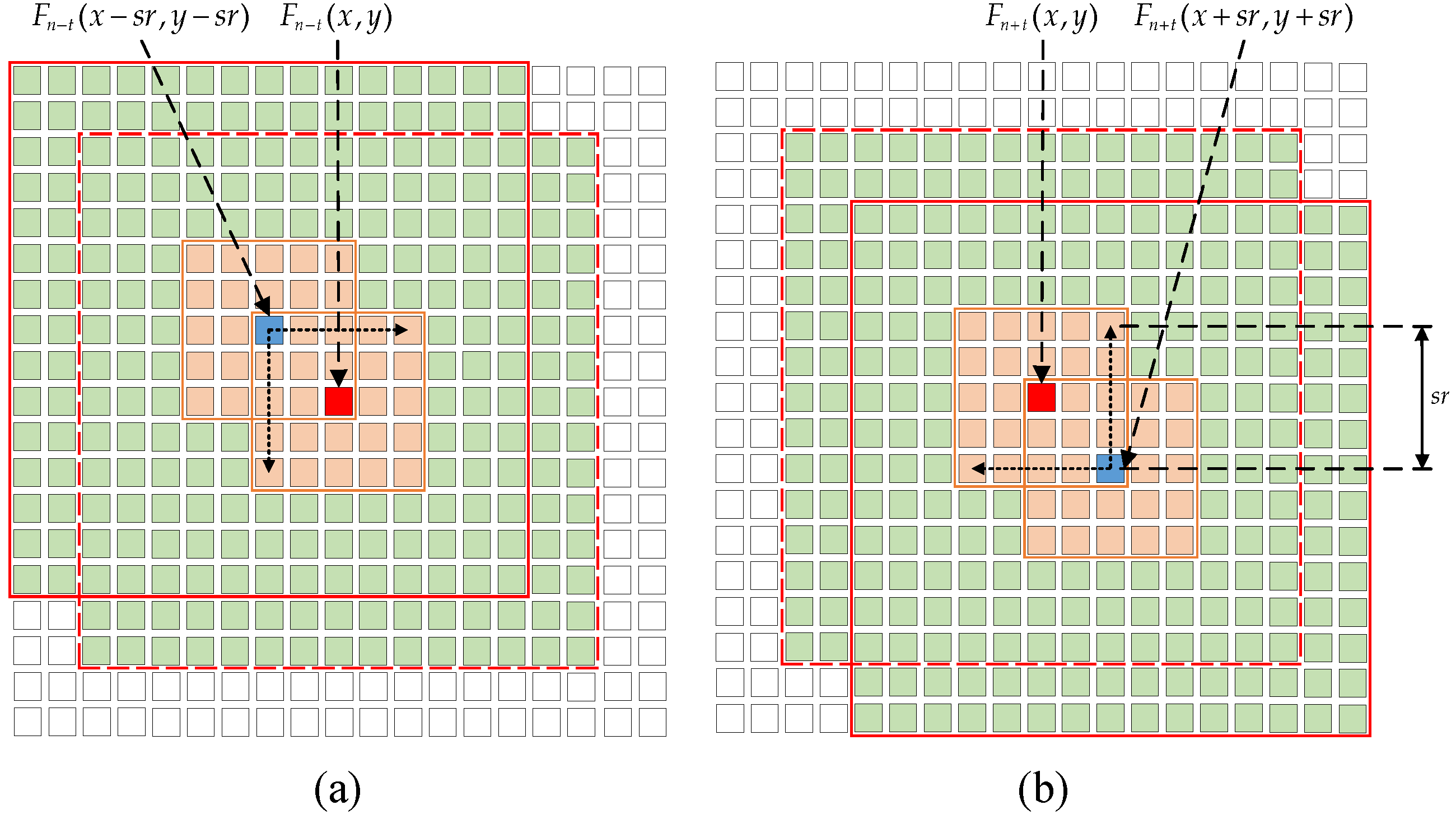
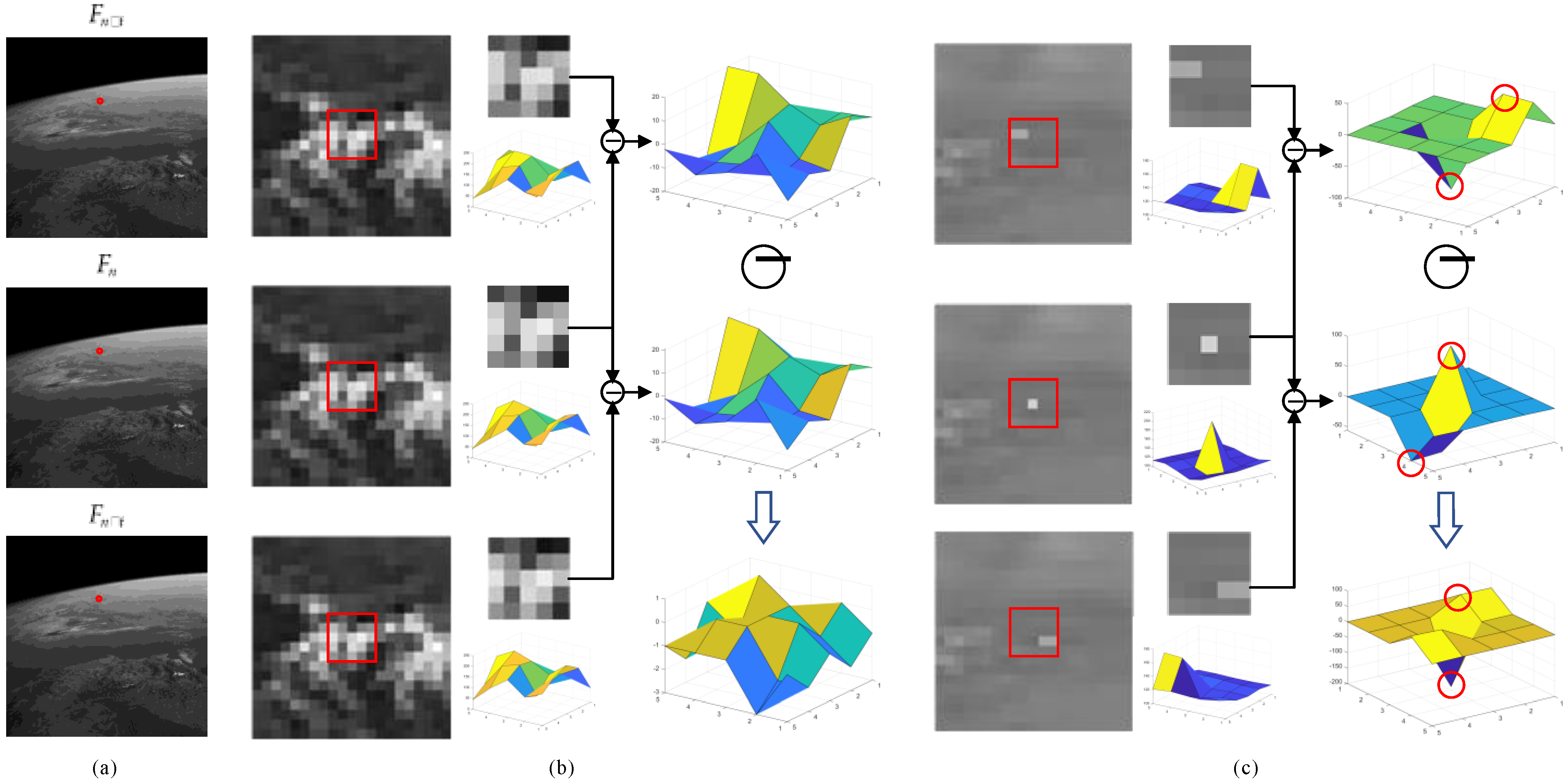
  • A local neighborhood spatial–temporal matching strategy is proposed, which estimates the local surrounding background motion model by registering local slices with a shielded center region.
  • A spatial–temporal difference enhancement map (STDEM) target enhancement factor is designed based on the spatial–temporal registration results. By analyzing the grayscale difference of the central matching blocks between the target and clutter, the STDEM extracts the positive and negative grayscale peaks of the difference results to strengthen the target energy.
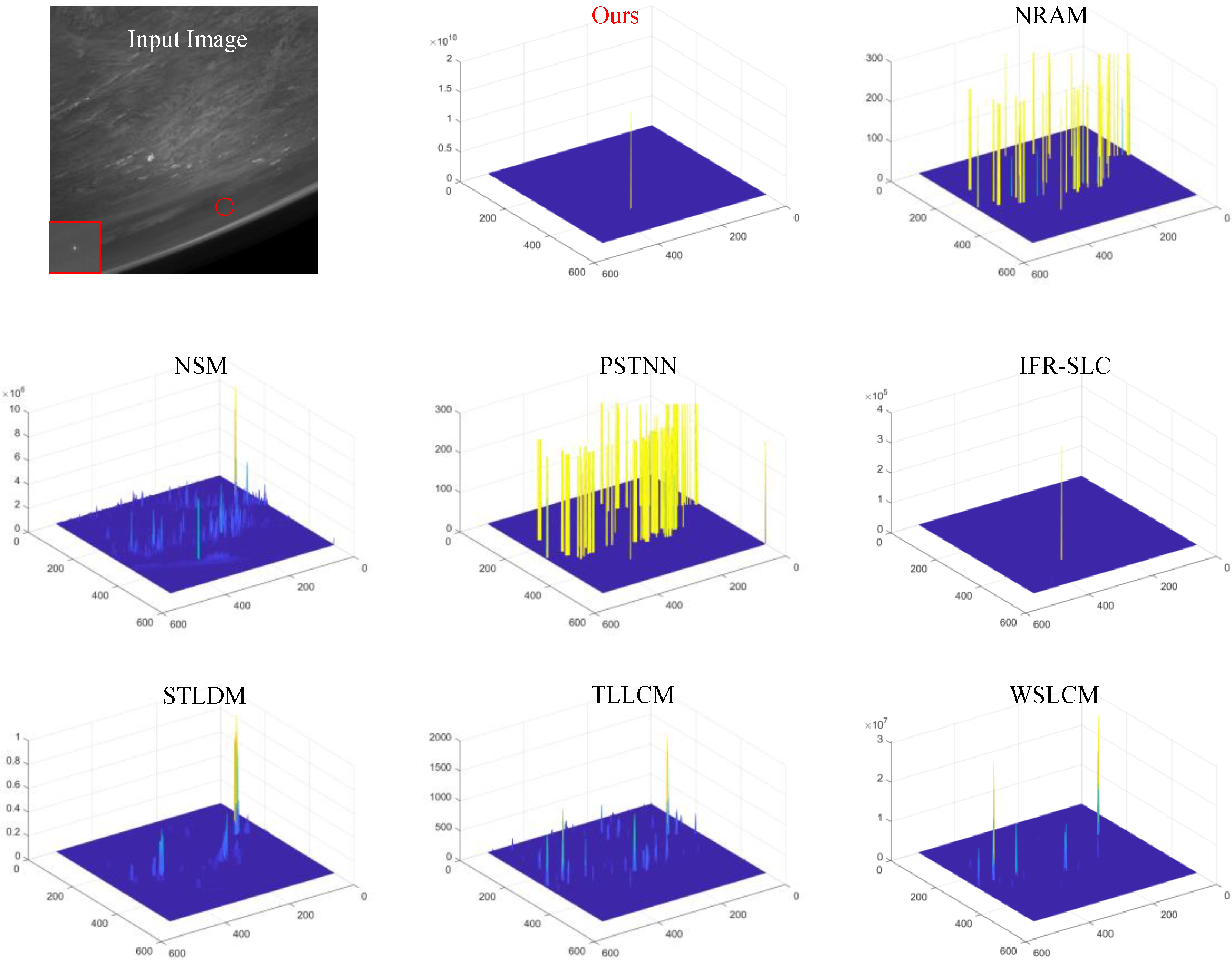
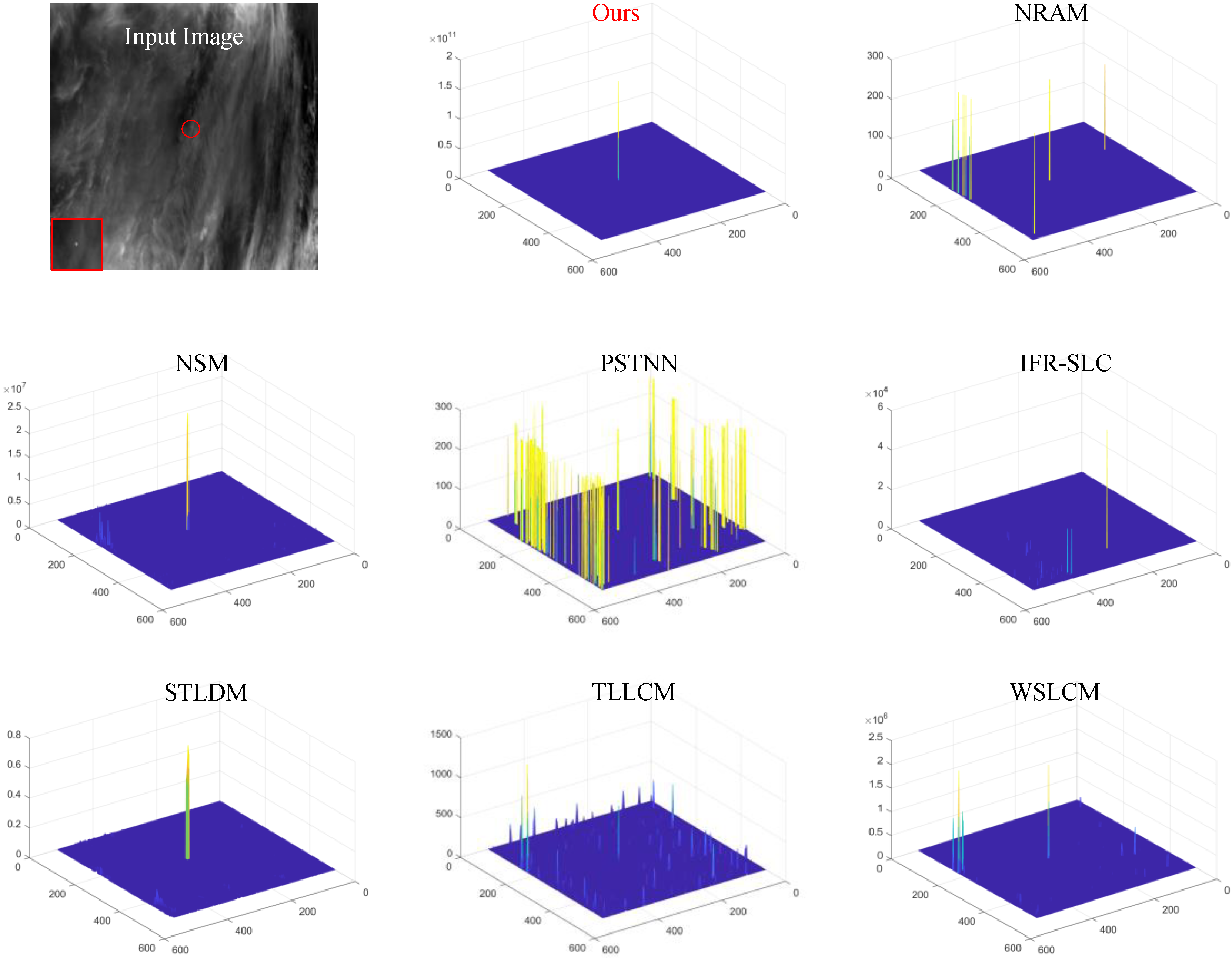
  • Extensive experiments are conducted on the simulated datasets synthesized by the actual optical image background. The experimental results show that the proposed method can filter most of the strong background clutter composed of ground surface and complicated clouds and has an excellent target detection performance in complex backgrounds.
The rest of this article is structured as follows: In Section 2, the proposed method is introduced in detail. Section 3 provides the results and analysis of the comparison experiments. The discussion and conclusion of this article are presented in Section 4 and Section 5, respectively.

2. Related Works

As a research hotspot in computer vision, numerous solutions have been developed for the weak- and dim-target detection problem, which can be broadly categorized into four types: image filtering-based, human visual contrast-based, optimization-based, and deep learning methods, as shown in Table 1.
The traditional research direction is the single-frame detection algorithm based on image filtering [11,12,13,14,15], which generally uses image filters to estimate and suppress the background. These algorithms utilize the grayscale information of pixels in the filtering window to estimate the image background and suppress background noise and clutter, but they may fail for strong background clutter points.
The mainstream small-target detection method is derived from the human visual system (HVS), which relies on target pattern characteristics of the ratio and difference types. The local contrast measure (LCM) [16] provides a basic target enhancement model. Various improved HVS algorithms [17,18,19,20,21,22,23,24] have been proposed, which usually involve weighted enhancement functions [19] or multi-layer filtering windows [20] or incorporate preprocessing operations [22] to increase detection accuracy, leading to a more intricate detector structure. Motivated by the temporal domain correlation, studies [25,26,27,28] have combined the spatial and temporal contrast features and proposed a spatial–temporal local contrast filter (STLCF) [25], interframe registration, and spatial local contrast (IFR-SLC) [27] and spatial–temporal local difference measure (STLDM) [28]. However, these algorithms cannot deal with the suppression of clutter that is similar to the target.
The optimization algorithm [29,30,31] has also been focused on, based on the data structure that segments targets based on the sparsity of small targets and the low-rank characteristics of the image background, such as the non-convex rank approximation minimization joint l2, 1-norm (NRAM) [30] and the partial sum of the tensor nuclear norm (PSTNN) [31]. Motivated by the temporal domain correlation, some improved optimization algorithms [32,33,34,35] incorporate temporal information into the tensor model to further separate the target from the background strong clutter. However, most optimized separation algorithms often perform iterative calculations, which requires considerable computing time and resources to achieve a better detection performance.
Furthermore, some deep learning algorithms [36,37,38,39] are also used to detect small targets. Qi et al. provided a fusion network of Transformer and a CNN (FTC-Net) [37], which extracts local detail features and global contextual features. Du et al. [38] proposed a spatial–temporal feature-based detection framework based on the interframe energy accumulation enhancement mechanism and used the small intersection over union (IOU) strategy to suppress the strong spatially non-stationary clutter. It is difficult for the deep learning method to learn features from small and weak targets with a sensitive size. Moreover, these methods often require a large amount of data, making them impractical for space-based applications.
By investigating the above literature, most existing algorithms focus on the ground scene, and there is little research on space moving-target detection in a space-based complex background. Detecting space moving targets submerged in complex backgrounds remains a critical challenge.

3. Methodology

The framework of the proposed local spatial–temporal registration method is illustrated in Figure 1. First, local neighborhood spatial–temporal matching is conducted on the selected three-frame images to estimate the motion vector of the local neighborhood. Then, we extract the spatial–temporal matching center block based on the background motion vector and conduct the difference operation to obtain the STDEM. Further, to acquire the TPCM, we calculate the background image using the matching results and the reference frame image and analyze the residual image after removing the background from the base frame. Finally, the classical threshold segmentation algorithm is applied to the LSTR map generated by combining the above two enhancement factors to extract the target.

3.1. Local Neighborhood Spatial–Temporal Matching

Let F 1 , , F n l , , F n , , F n + l , , F m be a space target image sequence, in which F n denotes the currently processed frame image in the sequence and F n + l represents the currently processed frame image with a backward interval of l frames. To create an image group,   { F n t , F n , F n + t } , we select the reference frame according to the frame interval ( t ) for the currently processed base frame ( F n ). The local neighborhood block matching will be conducted on this image group.
Under the space-based surveillance platform, space images usually contain the ground surface and the deep space background. Hot spots on the Earth and cloud clutter are the primary background interference influencing the target detection. In a single-frame image, distinguishing between space targets and ground targets can be challenging. However, in sequence images, ground targets move with the surrounding ground background, while space targets move according to their orbits, resulting in differences in motion speed and direction in the images. Meanwhile, the reflected light from space targets is relatively consistent, and the bright cloud reflection point and ground clutter point may change dramatically from a temporal perspective.
In this study, we utilize spatial–temporal correlation and motion model differences between the space target and the background clutters on Earth caused by the different orbital altitudes to suppress clutter and enhance targets. In brief, the motion model of the background and target remains stable in a short time for continuous images but slightly differ due to their respective trajectories.
According to the characteristics above, we simulated the simplified motion diagram of the target and surrounding clutter, as illustrated in Figure 2. The red square representing the target moves as the blue arrow indicates, and the blue squares denoting the background clutter move as the black arrow indicates. The proposed algorithm first estimates the neighbor background motion model by the spatial–temporal matching of the surrounding neighborhood. Then, we extract the temporal matching center block group according to the registration results and analyze the difference in the block group in grayscale intensity. As shown in the central region with orange pixels in Figure 2, the blue background clutter point position is consistent in the matched central block group, while the red target point position varies. Subsequently, we use this difference characteristic to enhance the target and suppress the background noise.
For the pixel ( x , y ) in the base frame ( F n ), we segment the registration slice around the pixel and set the center region as zero, where the target may exist. The specific matching operation is as follows:
First, an image patch ( B l ) is split for the pixel ( x , y ) in the base frame ( F n ), as shown in Figure 3. The formula of the image patch B l , n is defined as follows:
B l , n = { ( i , j ) | max i x , j y b r }
where ( i , j ) is the pixel coordinate in F n , b r means the half-size of the image patch ( B l , n ) with a recommended range of 5~10.
To shield the central region that may contain the target and accurately estimate the motion model of the neighborhood background, we multiply the image patch ( B l , n ) by the slice mask ( B m ) to form a neighborhood matching block ( B n ), and the formula is as follows:
B n = B l , n × B m
B m p , q = 0 ,   max p b r , q b r t r 1 ,   otherwise
where p , q is the pixel coordinate in the slice mask ( B m ), b r denotes the half-size of the slice mask ( B m ), and t r indicates the half-size of the center region with the recommended range of 1~3. After that, the grayscale intensity of pixels in the central region of the slice is set to 0, and the other pixels are retained.
Then, centered around the pixel ( x , y ) in the reference frame, a neighborhood matching block group of the same size as the matching block ( B n ) is segmented within the search step size ( s r ), and the pixel of the central region is set to zero. The similarity between the neighborhood matching block group and block B n is calculated to confirm the most similar matched block with block B n and estimate the neighborhood background motion model.
The search direction of the matching block for the reference frames F n t and F n + t , is shown in Figure 4.
As shown in Figure 4a, we extract the local surrounding background matching block ( B n t k 1 , k 2 ) of F n t . The formula is as follows:
B n t k 1 , k 2 = B l , n t k 1 , k 2 × B m , k 1 = k 2 = s r , , s r
B l , n t k 1 , k 2 = { ( i , j ) | max i ( x + k 1 ) , j ( y + k 2 ) b r }
where ( i , j ) is the pixel coordinate in the reference frame ( F n t ), b r is the half-size of the slice ( B n t k 1 , k 2 ), s r is the half-size of the search matching range, and ( k 1 , k 2 ) is the displacement of slice ( B l , n t k 1 , k 2 ) center coordinate relative to ( x , y ) , ranging from s r to s r . The search starting point of the local neighborhood background matching block ( B l , n t k 1 , k 2 ) for F n t is ( x s r , y s r ) .
Meanwhile, the similarity coefficient ( r n t k 1 , k 2 ) between the background matching blocks of the base frame and the reference frame is calculated. The formula is as follows:
r n t k 1 , k 2 = i , j B n i , j × i , j B n t k 1 , k 2 i , j i , j B n i , j 2 i , j B n t k 1 , k 2 i , j 2 , k 1 = k 2 = s r , , s r
Furthermore, as shown in Figure 4b, we extract the local neighbor background matching block ( B n + t k 1 , k 2 ) for F n + t by referring to Formulas (4) and (5). The similarity coefficient ( r n + t k 1 , k 2 ) of the neighboring matching block ( B n ) and B n + t k 1 , k 2 is calculated using Formula (6). The search starting point position of the local neighborhood background matching block in the reference frame ( F n + t ) is ( x + s r , y + s r ) , which is different from the F n t .
Finally, we integrate the matching results of the reference frame and calculate the enhanced similarity matrix ( r n k 1 , k 2 ) to estimate the motion model of the local background accurately. The formula is as follows:
r n k 1 , k 2 = r n t k 1 , k 2 + r n + t k 1 , k 2
Based on the enhanced similarity matrix ( r n k 1 , k 2 ), we identify the search number with the maximum similarity coefficient value as the direction and displacement of the local neighborhood background motion at the pixel. The formula is as follows:
d x , d y = a r g m a x r n k 1 , k 2 , k 1 = k 2 = s r , , s r
where d x , d y represent the local neighborhood background motion vector in the X-axis and Y-axis direction, respectively. The registration operation is applied to each pixel in F n , calculating the neighbor background motion model for the entire image.

3.2. Spatial–Temporal Difference Enhancement Map Calculation

In this step, the analysis of spatial–temporal difference is conducted on the temporal matching center blocks based on the local neighborhood motion model. By analyzing the temporal grayscale difference between the strong clutter and the target, it can be seen that the strong clutter moves with the overall Earth background in the image sequences, and the grayscale distribution of the background clutter matched by the estimated neighbor background motion model is similar. However, the target area will move relative to the background, and the grayscale distribution of the target region matched by the estimated neighbor background motion model will differ. The difference operation is as follows:
First, the center block ( T n ) of the pixel x , y is extracted from the base frame ( F n ). The T n is defined as
T n = { ( i , j ) | max i x , j y t r }
where ( i , j ) is the pixel coordinate in the base frame ( F n ); t r is the half-size of the center block T n .
Then, based on the local neighborhood motion vector d x , d y , we separate the center blocks T n t and T n + t from the reference frames F n t and F n + t , respectively. The formulas of T n t and T n + t are defined as follows:
T n t = { ( i , j ) | max i ( x + d x ) , j ( y + d y ) t r }
where ( i , j ) is the pixel coordinate in the reference frame F n t .
T n + t = { ( i , j ) | max i ( x d x ) , j ( y d y ) t r }
where ( i , j ) is the pixel coordinate in frame F n + t . We call these three extracted blocks the temporal matching center block group.
According to the previous analysis, when there is clutter interference in the central region block with the same motion vector as its neighbor background, the temporal matching center block group will show the same distribution of grayscale intensity, as shown in Figure 5b. The maximum grayscale location of this temporal matching center block group is different when it contains a target in the center region, as illustrated in Figure 5c. After the center block difference operation, the difference result of the clutter region will be low and close to zero. There will be a positive and negative peak pair with an enormous difference in the result of the target region. The STDEM extracts the positive and negative grayscale peaks of the difference results to shorten the strong clutter and highlight the target. The specific calculation is as follows:
We first perform a frame difference operation for the center block ( T n ) to obtain the difference block ( d 1 , d 2 ) . The formula is defined as follows:
d 1 = T n t T n
d 2 = T n T n + t
After the difference operation, the signal energy of the target region is retained, and a group of positive and negative peak pairs is generated in the target region difference block, as shown in Figure 5c. As shown in Figure 5b, the strong background clutter can be suppressed since the pixel grayscale intensity of the difference result is lower in the clutter region.
Further, difference block d 3 between d 1 and d 2 is calculated to restrain the residual interference of highlighted clutter. The formula of d 3 is defined as follows:
d 3 = d 1 d 2
As shown in Figure 5b,c, after the enhanced difference operation, the grayscale intensity of the pixel is closer to 0, and the signal energy of the target is further enhanced.
We calculate the STDEM by extracting the positive and negative peak pairs for the spatial–temporal local difference results ( d 3 ). The formula of STDEM is as follows:
S T D E M x , y = ( max d 3 min ( d 3 ) ) 2
After the above enhancement calculation of grayscale intensity difference, if the background clutter appears at the pixel x , y , the value of S T D E M x , y is lower. In contrast, the grayscale intensity difference extraction operation can obtain a higher value of S T D E M x , y when a target exists at the pixel x , y .

3.3. Temporal Pixel Contrast Map Calculation

In this step, the pixel-level temporal contrast map is calculated to suppress background clutter further. Although the background clutter of continuous image sequences has a temporal correlation, the long detection distance inevitably leads to slight changes in the shape of the background clutter between continuous image frames, which may lead to a strong energy signal in the STDEM. The temporal pixel contrast map is a more accurate pixel difference operation based on the estimation results of the local background motion model to suppress the background clutter with interframe morphological changes.
Specifically, we use the matching results of the neighborhood background to conduct temporal differential calculations for each pixel. Then, a matching residual image is generated, suppressing the residual clutter generated by the above phenomenon.
First, we use the local neighborhood motion vector ( d x , d y ) to obtain a residual image. The specific formula is as follows:
P e x , y = F n x , y F n b x , y
F n b x , y = [ F n t x + d x , y + d y + F n + t x d x , y d y ] / 2
where P e x , y is the value of the pixel coordinate x , y in the matching residual image ( P e ), F n denotes the base frame, F n t and F n + t denote the reference frame, and ( d x , d y ) mean the local neighborhood motion vector of the pixel coordinate x , y .
From the formula above, the pixel-level time-domain difference of the image frame may be understood as the difference between the base frame ( F n ) and the predicted background image ( F n b ) estimated by the reference frame and the local neighbor motion vector. The high-brightness clutter points can be suppressed by matching the corresponding background pixels in the reference frame. In contrast, the target center energy is retained by matching to the neighbor background points. The residual image is displayed in Figure 6c. It can be seen from the 3D view of the residual image that the grayscale intensity of the target region is retained and positive. The residual image in the clutter region may give a negative value due to the temporal grayscale intensity change. However, the residual grayscale value in the clutter region is distributed close to 0. To avoid negative values in subsequent calculations, we set the negative value in the residual image to 0 to obtain the temporal pixel contrast map, as shown in Figure 6d. The formula of the temporal pixel contrast map (TPCM) is shown as follows:
T P C M x , y = P e x , y , P e x , y > 0 0 ,   otherwise
where T P C M x , y is the value of the pixel coordinate x , y in the TPCM.

3.4. Local Spatial–Temporal Registration Map Calculation

Finally, we combine the spatial–temporal difference enhanced map (STDEM) and temporal pixel contrast map (TPCM) to calculate the LSTR map to separate the target from the surrounding background noise. The formula is as follows:
L S T R ( x , y ) = S T D E M ( x , y ) × T P C M ( x , y )
where L S T R ( x , y ) is the value of the pixel coordinate ( x , y ) in the LSTR map. The target saliency map shows a high target signal and low background energy. The adaptive threshold segmentation algorithm, which uses the image average and standard deviation to calculate a specific threshold for target segmentation, can boost the precision of target detection of the image sequences. The threshold is calculated as follows.
T h = μ + k × σ
where μ denotes the average value of the LSTR map, σ represents the standard deviation value of the LSTR map, and k is the adaptive segmentation threshold. The range of this threshold parameter, which ranges from 200 to 300, is effective in this study.

4. Experiment and Analysis

This section first discusses the experimental datasets used in this study. Then, a group of 3D receiver operating characteristic (ROC) curve-derived detection metrics are presented to assess the effectiveness of the proposed method. Finally, a comprehensive analysis is provided based on the qualitative and quantitative results. We conducted all of the experiments on a computer with 16 GB of RAM and an Inter Core i7-10750H CPU 2.60 GHz processor.

4.1. Experimental Datasets

In this study, we conducted tests on four image sequences sized 512 × 512 with different backgrounds to evaluate the effectiveness and robustness of the proposed method. The experimental datasets were synthesized by actual space-based short-wave infrared and visible-light background image sequences and simulated space moving targets. The background image data used in this test were derived by decomposing a public video of the Earth from a space perspective. Seq.1 and Seq.2 were simulated based on the motion trajectories and grayscale changes of the targets in the real space target image sequences. The details of the experimental datasets are listed in Table 2. There is a space moving target in each group of image sequences. In detail, Seq.1 and Seq.4 have a similar background that contains the high-contrast edge of the Earth and bright-point ground clutter. Seq.2 simulates the space-based tracking mode where the target remains motionless and the background image is a stationary cloudy landscape. Seq.3 has a background comprising complex ground clusters, cloud clutter, and bright pixel-sized noise. The signal-to-clutter ratio (SCR) evaluates the background clutter intensity by calculating the ratio of the target signal to its neighboring noise distribution level. The lower the signal-to-clutter ratio, the more it challenges the target enhancement and clutter suppression capabilities of the proposed algorithm. The S C R is defined as follows:
S C R = ( μ t μ b ) / σ b
where μ t denotes the average of the target region; μ b and σ b are the average and standard deviation of the neighboring background, respectively.

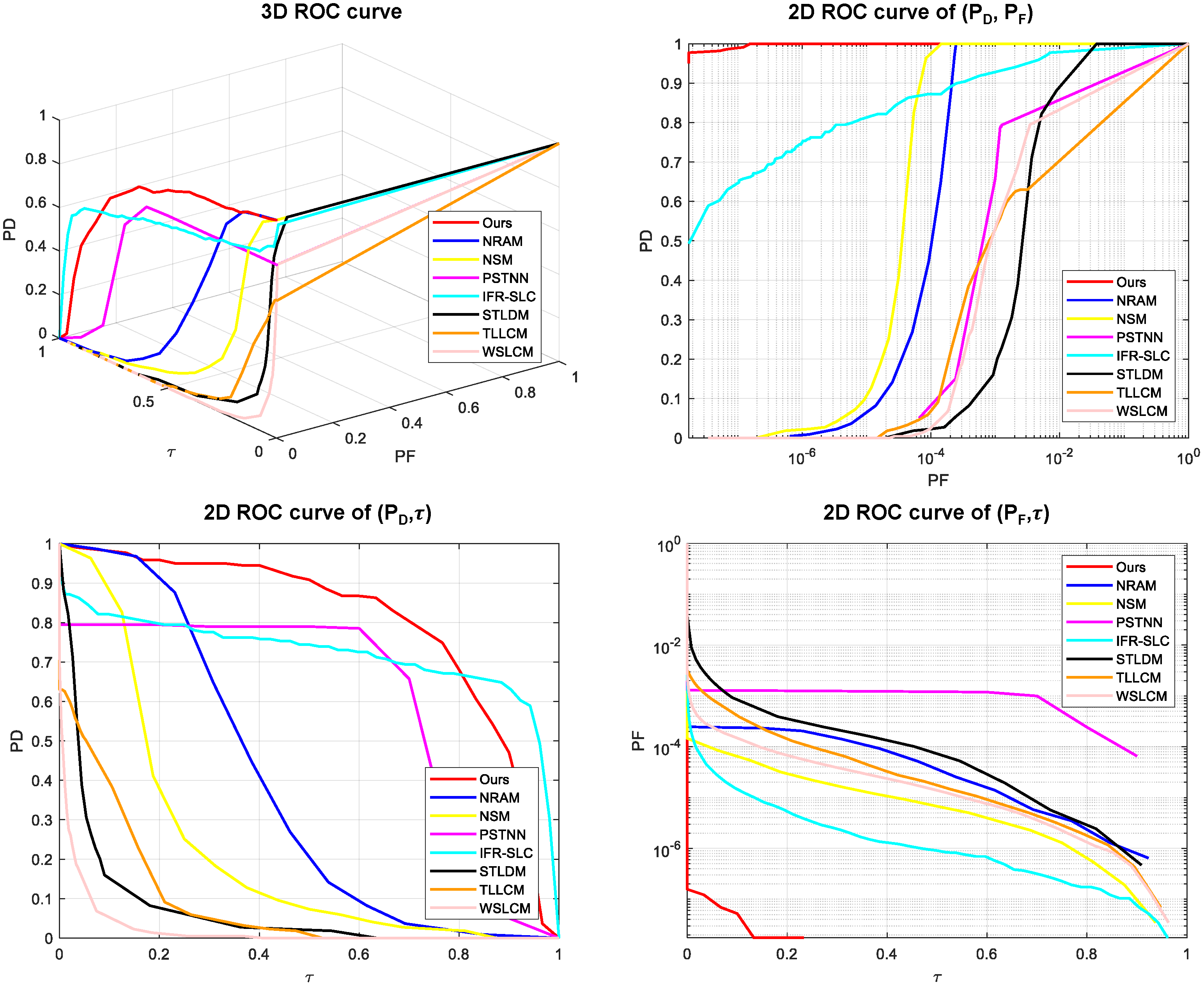
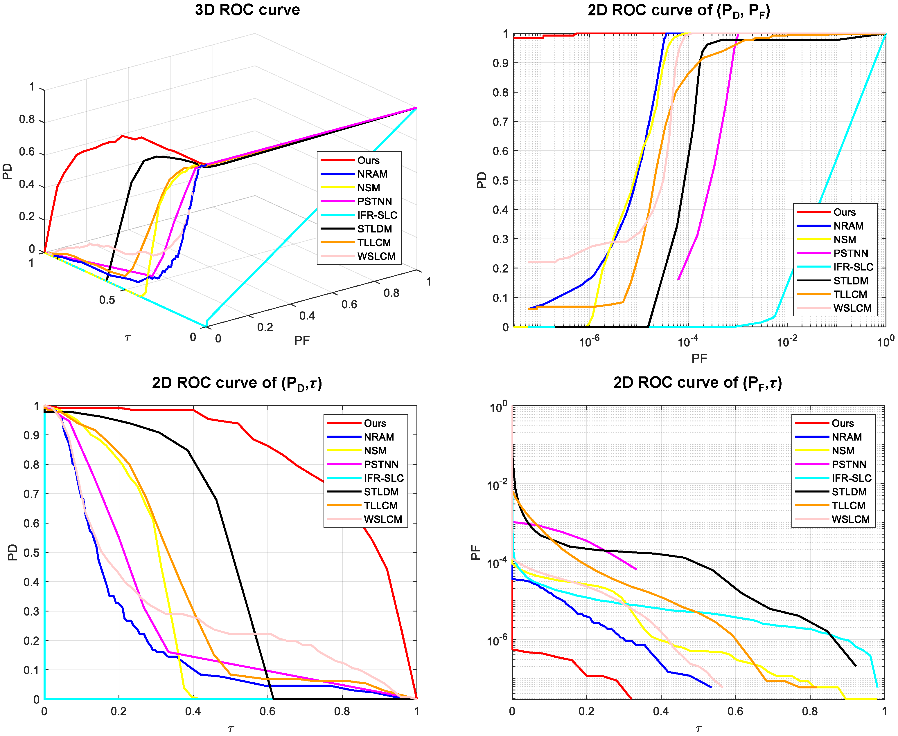
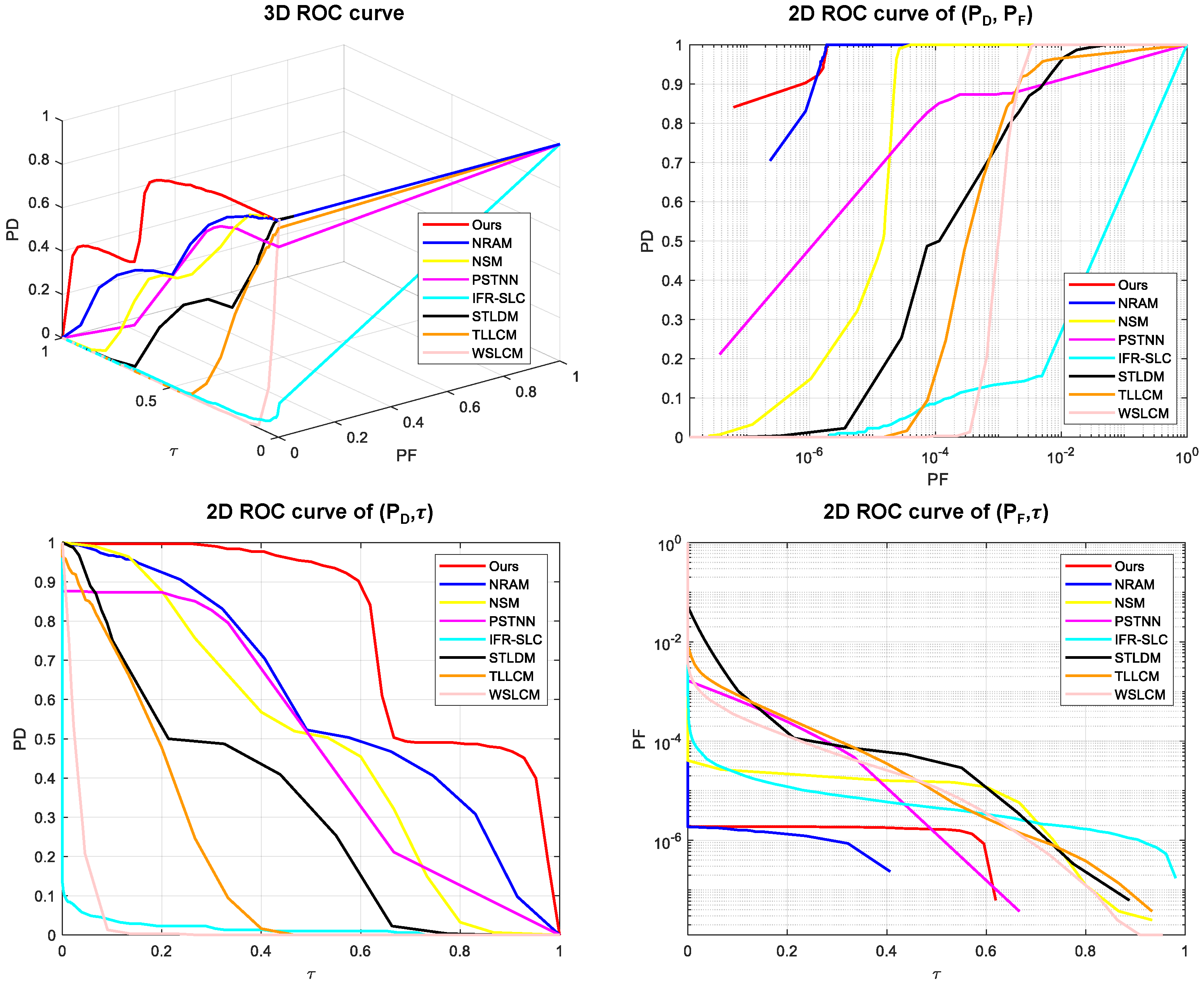
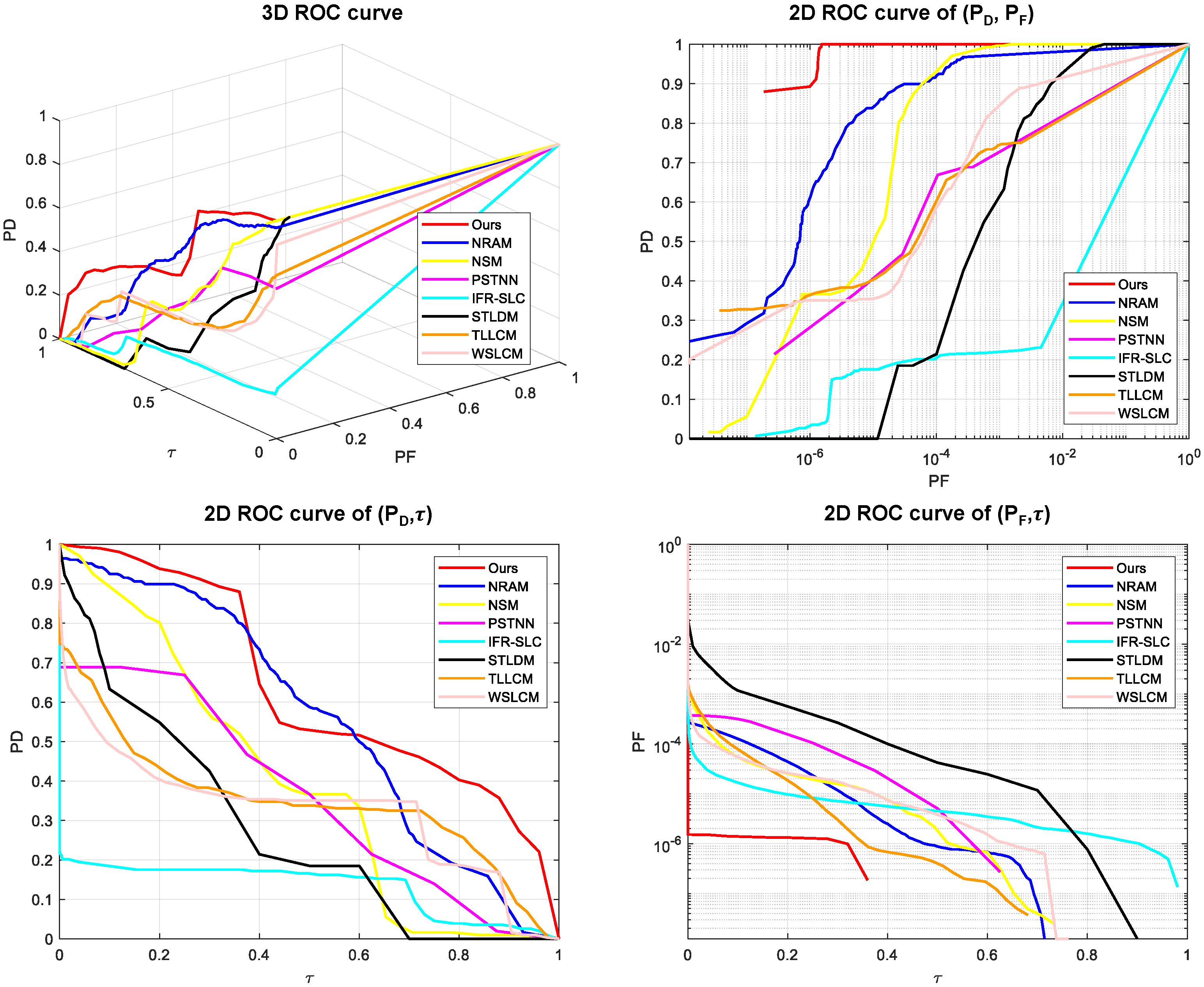
4.2. Evaluation Metrics

The detection probability ( P D ) and false alarm rate ( P F ) are the primary evaluation indicators that can accurately quantify the detection performance. The formulas of P D and P F are given as follows:
P D = N d / N t
P F = N f / N p
where N d is the number of detected targets, N t is the number of real targets, N f is the number of false detected targets, and N p is the total pixel number of the image. In addition, the target enhancement and background suppression abilities are the commonly used evaluation indicators to measure the effectiveness of the detector, since boosting the target signal increases the target detection probability. Existing research employs the signal–noise ratio gain (SNRG), the background suppression factor (BSF), the ROC curve of P D and P F , and the area under the ROC curve (AUC) to assess the detector. However, the calculation of SNRG and the BSF relies on the statistics of the local standard deviation of the detection results, which may produce misleading statistics caused by ambiguous values. The ROC curve ( P D , P F ) may produce the same result when calculating the AUC value that cannot provide persuasive comparison results.
Chang et al. [40] proposed a three-dimensional ROC (3D-ROC) analysis tool and a group of related detection indicators to address the abovementioned issues, extending the conventional 2D ROC curve ( P D , P F ) by introducing the threshold, τ . Three 2D ROC curves ( P D , P F ) , ( P D , τ ) , and P F , τ , can be separated from the 3D-ROC curve ( P D , P F , τ ) using the threshold τ . The closer the ROC curve ( P D , P F ) is to the upper left corner, the better the detection effect of the detector; the closer the ROC curve ( P D , τ ) is to the upper right corner, the better the detection effect of the detector; the closer the ROC curve P F , τ is to the lower left corner, the better the background suppression effect of the detector. Simultaneously, the three 2D ROC curves can be utilized to conduct the calculation of extended eight AUC metrics, including A U C ( D , F ) , A U C ( D , τ ) , A U C ( F , τ ) , A U C T D , A U C B S , A U C T D B S , A U C O D P , and A U C S N P R . A U C ( D , F ) is the AUC value of the ( P D , P F ) ROC curve. A U C ( D , τ ) is the AUC value of the ( P D , τ ) ROC curve. A U C ( F , τ ) is the AUC value of the P F , τ ROC curve. A U C T D , A U C B S , A U C T D B S , A U C O D P , and A U C S N P R are, respectively, the evaluation index of target detection (TD), background suppression (BS), joint evaluation, overall detection probability (ODP), and signal-to-noise probability ratio (SNPR). They are defined as follows:
A U C T D = A U C ( D , F ) + A U C ( D , τ )
A U C B S = A U C ( D , F ) A U C ( F , τ )
A U C T D B S = A U C ( D , τ ) A U C ( F , τ )
A U C O D P = A U C ( D , F ) + A U C ( D , τ ) A U C ( F , τ )
A U C S N P R = A U C ( D , τ ) / A U C ( F , τ )

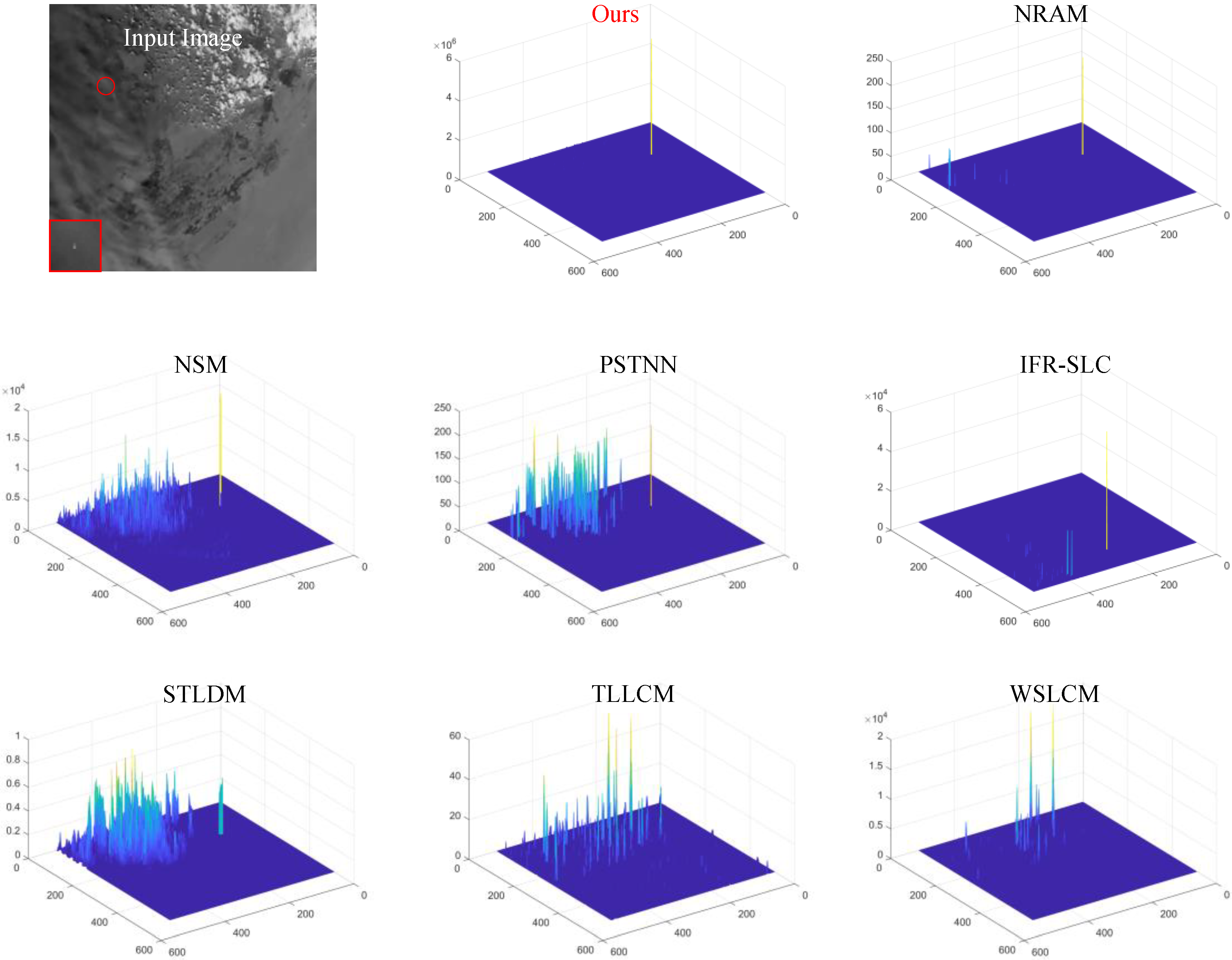
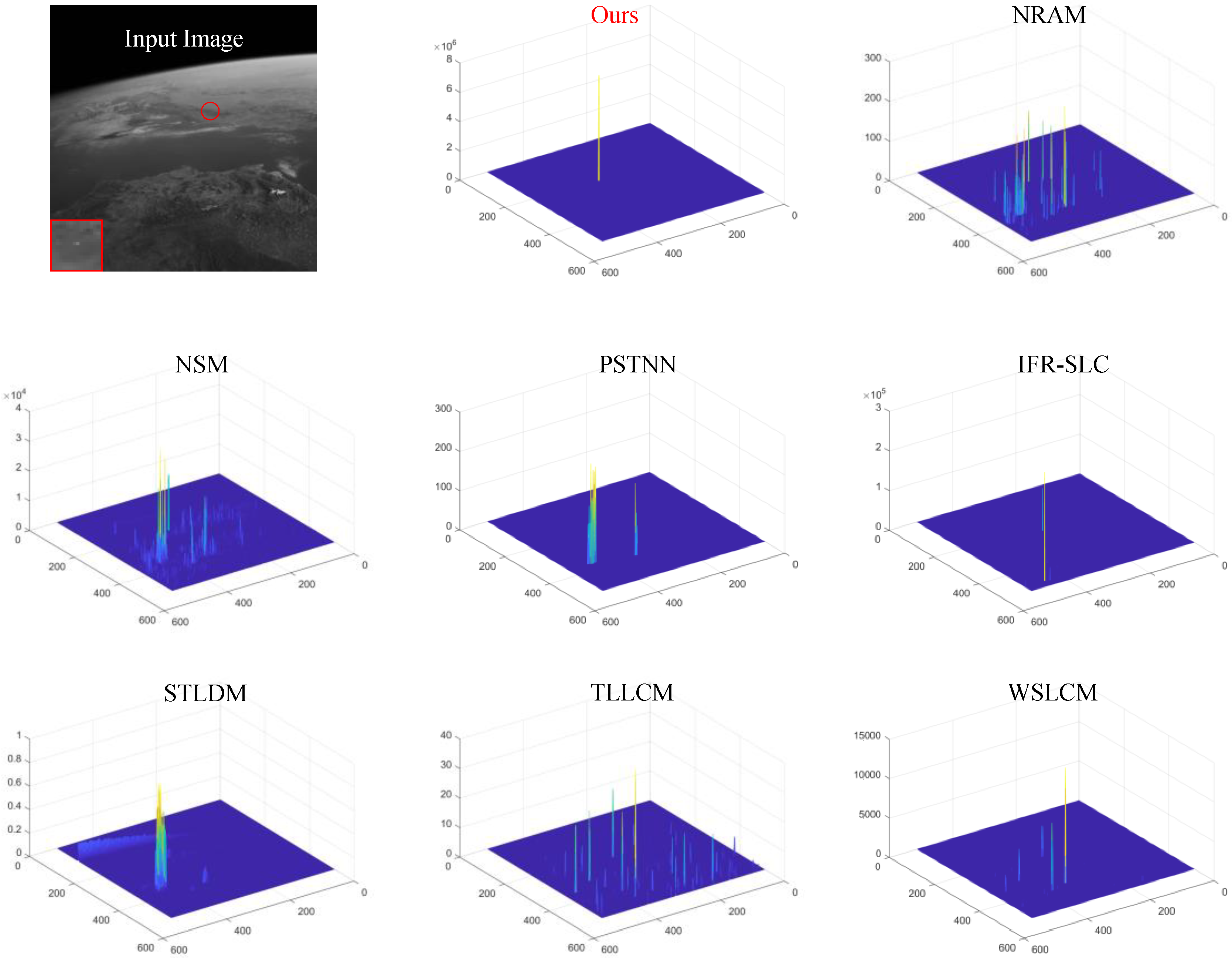
4.3. Comparative Experiments

This research compares seven state-of-the-art detection methods to verify the detection performance of the proposed algorithm. Three HVS-based single-frame detection algorithms are included in the comparison methods: WSLCM, NSM, and TLLCM. We also compare two HVS-based methods combining spatial and temporal feature information, IFR-SLC and STLDM. Furthermore, two optimization algorithms based on data structure, NRAM and PSNN, are also used for comparison as they have solid background suppression capabilities. Table 3 provides the parameter settings for the comparison algorithms.
A saliency map of four datasets processed by the comparative methods is shown in Figure 7, Figure 8, Figure 9 and Figure 10. The red circles indicate the target’s position in the input image. The detection results of the image in Seq.1 are shown in Figure 7. The target cannot be recognized since the NRAM and PSTNN algorithms boost the clutter and the target to the same degree. NSM, STLDM, TLLCM, and WSLCM can enhance the target, but they are much more sensitive to clutter. Only the proposed method and IFR-SLC achieve a better target enhancement and clutter suppression performance. The background clutter distribution in Seq.4 is similar to Seq.1, and only the proposed algorithm showed a convincing performance, while other algorithms failed to separate the target from the clutter. In Seq.2, as shown in Figure 8, the cloud clutter distribution in the background appears smooth and uniform. In the detection results of NSM, STLDM, NARM, and WSLCM, the target signal energy is accurately enhanced, but some point-sized clutter noise remains. Cloud clutter interference influenced PSTNN, IFR-SLC, and TLLCM. The proposed method can suppress cluttered backgrounds and highlight targets more effectively. The background of Seq.3 is a non-stationary intense clutter scenario, as shown in Figure 9. All comparative methods failed to suppress the fragmented cloud clutter besides the proposed method and NRAM. The experimental results demonstrated that the proposed method performs satisfactorily in target enhancement and strong clutter suppression.
After conducting a qualitative analysis of the detection results, a quantitative analysis is also provided to evaluate the proposed algorithm further. The 3D ROC curve and three 2D ROC curves ( P D , P F ) , ( P D , τ ) , and P F , τ , for the experimental results are shown in Figure 11, Figure 12, Figure 13 and Figure 14. The evaluation indicators for the experimental datasets are listed in Table 4, and bolded and underlined data are the best and sub-best AUC results, respectively.
The image of the Seq.1 dataset contains a large number of bright ground hot-spot clutter with a shape distribution that closely resembles the target. In Table 4, the A U C ( D , F ) values of NRAM and NSM both reach 0.999. Although the A U C ( D , F ) value of IFR-SLC is not high, its joint evaluation index and overall detection probability are better than other algorithms. All indices of the proposed algorithm are superior to those of other algorithms, indicating that the algorithm can guarantee the detection rate of the target under heavy clutter interference.
For the Seq.2 dataset, the images are contaminated by the fluent cloud background clutter. It can be seen in Table 4 that the A U C B S values for the NRAM, NSM, and WSLCM algorithms reach 0.999, but they are not dominant in target detection, indicating that they have a better suppression effect on stable background clutter. The A U C O D P and A U C S N P R values of STLDM are higher than those of other comparative algorithms, demonstrating its ability to balance target detection and background suppression. The proposed approach demonstrates superior performance in all indices compared to comparative algorithms, exhibiting its ability to detect the target while accurately reducing stationary cloud background interference.
The images in Seq.3 are generated in a background containing many patches and spots of high-brightness cloud clutter and an uneven ground scene. Table 4 shows that the NSM has significantly higher values in the background suppression evaluation parameters than other algorithms and performs better in other comprehensive evaluation indicators. In addition, the evaluation of NRAM and our proposed algorithm are close, and the target detection index ( A U C T D ) of the proposed algorithm is slightly higher than that of the NRAM algorithm, indicating that both of them are suitable for small spatial target detection in scenes with non-stationary strong clutter and noise.
The image of Seq.4 contains a high-contrast Earth edge background and non-uniform background clutter points. In Table 4, both the NSM and STLDM obtain high background suppression effects. There are no significant differences between NARM and the proposed algorithm except for the background suppression evaluation index, A U C B S . As a result, the proposed algorithm can detect targets accurately in scenes with large grayscale fluctuations in the background. The NSM single-frame detection algorithm did not effectively utilize the temporal information of the target. However, with the preprocessing step of TDLMS, it can more efficiently suppress clutter noise in the image and reduce the occurrence of false alarms. While the IFR-SLC algorithm uses a frame registration strategy for target enhancement, it cannot solve the target detection problem in this research due to the limited application scenario. Additionally, NRAM and STLDM, which use spatial–temporal features, can effectively suppress most stationary background clutter. With high robustness and good detection performance, the proposed algorithm can adapt to detecting targets under different dynamic backgrounds.

5. Discussion

The comparative experiment proves the capacity to detect moving targets in complex backgrounds of the proposed algorithm from both a quantitative and qualitative perspective. This section provides an analysis of the parameter settings which influence the performance of proposed algorithms. Firstly, the frame interval ( t ) and search step size ( s r ) during the local neighborhood spatial–temporal matching stage affect the registration accuracy. The search step size in this research is set to three, meaning that the matching result may fail when the background motion speed of the image exceeds three pixels/frame. Thus, it is critical to set a suitable frame interval parameter to avoid a large displacement of the image background during neighboring region motion estimation. For example, when the background velocity is one pixel/frame, we recommend that the frame interval ( t ) does not exceed three.
Secondly, it is worth noting that the setting of the registration block size may affect the matching results. The recommended range of the registration block’s outer half-size ( b r ) is 5~10. If b r is less than the recommended range, the match operation in Section 3.1 may fail without enough background features. If b r is too high, the algorithm execution time in the registration stage may increase. The recommended range of the registration block’s inner half-size ( t r ) is one~three, depending on the target size. A smaller t r  may affect the prediction of the background motion state, whereas a larger  may interfere with the background matching. It also means that the proposed algorithm performs well in detecting small targets with a half-size of one~three. When the target is too large, the center pixel in the base frame may match the target edge pixel in the reference frame, which will weaken the target energy.
Furthermore, the extraction of the candidate target is affected by the adaptive segmentation threshold k for the saliency map. It is essential to analyze the impact of parameter k values on P D and P F . Figure 15 exhibits the variation trend of the P D and P F under different k values. It can be seen from Figure 15 that both the P D and P F increase as the k value decreases. The P D obtained from the four experimental datasets can reach 95% when k is less than 300. When the value of k decreases from 200 to 0, P F will be greater than 10−5 and produce exponential growth. Thus, the value of k is recommended to be [200, 300] to reach a P D > 95% with P F < 10−5.

6. Conclusions

This study proposes a local spatial–temporal registration method for space small-moving-target detection under complex scenes. A local neighborhood temporal matching strategy is introduced to calculate local surrounding background motion vectors based on the temporal correlation of the background features. Then, we analyze the temporal grayscale difference of the center region and calculate the spatial–temporal difference enhanced map using the motion model of the neighborhood background. After the background prediction and difference, the time-domain pixel contrast map that preserves the target signal and suppresses clutter energy is also obtained. Finally, the LSTR map is constructed by synthesizing the two enhancement factors. Qualitative and quantitative analyses of the experimental results prove that our proposed algorithm has better target enhancement and background suppression capabilities than other methods.
However, the proposed method is still limited, as it does not apply to scenes where the background clutter undergoes rapid changes, and it is also time-consuming. When the background grayscale distribution around the target changes dramatically in the time domain, the algorithm cannot use the neighborhood feature information to conduct the spatial–temporal match, which may fail detection. In future work, we will verify the detection performance of the proposed method in other complex scenes and conduct algorithm optimization to solve the mismatch problem caused by the sudden change in the interframe background. We will also try to deploy the proposed algorithm on onboard processing platforms to realize real-time space target detection and provide decision support for in-orbit evasion.

Author Contributions

Conceptualization, P.R. and Y.S.; methodology, Y.S. and X.C.; software, Y.S.; validation, Y.S., X.C. and F.L.; formal analysis, Y.S.; investigation, C.C.; resources, Y.S.; data curation, X.C.; writing—original draft preparation, Y.S.; writing—review and editing, X.C.; visualization, C.C.; supervision, P.R.; project administration, X.C.; funding acquisition, P.R. All authors have read and agreed to the published version of the manuscript.

Funding

This research received no external funding.

Data Availability Statement

Data are contained within the article.

Conflicts of Interest

The authors declare no conflicts of interest.

References

  1. Maclay, T.; Mcknight, D. Space environment management: Framing the objective and setting priorities for controlling orbital debris risk. J. Space Saf. Eng. 2021, 8, 93–97. [Google Scholar] [CrossRef]
  2. Kennewell, J.; Vo, B.-N. An overview of space situational awareness. In Proceedings of the 2013 16th International Conference on Information Fusion, Istanbul, Turkey, 9–12 July 2013; pp. 1029–1036. [Google Scholar]
  3. Wang, X.; Li, F.; Xin, L.; Ma, J.; Yang, X.; Chang, X. Moving targets detection for satellite-based surveillance video. In Proceedings of the IGARSS 2019-2019 IEEE International Geoscience and Remote Sensing Symposium, Yokohama, Japan, 28 July–2 August 2019; pp. 5492–5495. [Google Scholar]
  4. Su, Y.; Chen, X.; Liu, G.; Cang, C.; Rao, P. Implementation of Real-Time Space Target Detection and Tracking Algorithm for Space-Based Surveillance. Remote Sens. 2023, 15, 3156. [Google Scholar] [CrossRef]
  5. Zhou, D.; Wang, X. Stray Light Suppression of Wide-Field Surveillance in Complicated Situations. IEEE Access 2023, 11, 2424–2432. [Google Scholar] [CrossRef]
  6. Guo, X.; Chen, T.; Liu, J.; Liu, Y.; An, Q. Dim Space Target Detection via Convolutional Neural Network in Single Optical Image. IEEE Access 2022, 10, 52306–52318. [Google Scholar] [CrossRef]
  7. Xue, D.; Sun, J.; Hu, Y.; Zheng, Y.; Zhu, Y.; Zhang, Y. Dim small target detection based on convolutinal neural network in star image. Multimed. Tools Appl. 2020, 79, 4681–4698. [Google Scholar] [CrossRef]
  8. Lin, B.; Yang, X.; Wang, J.; Wang, Y.; Wang, K.; Zhang, X. A robust space target detection algorithm based on target characteristics. IEEE Geosci. Remote Sens. Lett. 2021, 19, 3080319. [Google Scholar] [CrossRef]
  9. Zhang, L.; Rao, P.; Hong, Y.; Chen, X.; Jia, L. Infrared Dim Star Background Suppression Method Based on Recursive Moving Target Indication. Remote Sens. 2023, 15, 4152. [Google Scholar] [CrossRef]
  10. Zhang, Y.; Chen, X.; Rao, P.; Jia, L. Dim Moving Multi-Target Enhancement with Strong Robustness for False Enhancement. Remote Sens. 2023, 15, 4892. [Google Scholar] [CrossRef]
  11. Bai, X.; Zhou, F. Analysis of new top-hat transformation and the application for infrared dim small target detection. Pattern Recognit. 2010, 43, 2145–2156. [Google Scholar] [CrossRef]
  12. Drummond, O.E.; Deshpande, S.D.; Er, M.H.; Venkateswarlu, R.; Chan, P. Max-mean and max-median filters for detection of small targets. In Proceedings of the Signal and Data Processing of Small Targets 1999, Orlando, FL, USA, 27–29 March 1999; pp. 74–83. [Google Scholar]
  13. Cao, Y.; Liu, R.; Yang, J. Small target detection using two-dimensional least mean square (TDLMS) filter based on neighborhood analysis. Int. J. Infrared Millim. Waves 2008, 29, 188–200. [Google Scholar] [CrossRef]
  14. Wang, C.; Wang, L. Multidirectional ring top-hat transformation for infrared small target detection. IEEE J. Sel. Topics Appl. Earth Observ. Remote Sens. 2021, 14, 8077–8088. [Google Scholar] [CrossRef]
  15. Li, Y.; Li, Z.; Zhang, C.; Luo, Z.; Zhu, Y.; Ding, Z.; Qin, T. Infrared maritime dim small target detection based on spatiotemporal cues and directional morphological filtering. Infrared Phys. Technol. 2021, 115, 103657. [Google Scholar] [CrossRef]
  16. Chen, C.P.; Li, H.; Wei, Y.; Xia, T.; Tang, Y.Y. A local contrast method for small infrared target detection. IEEE Geosci. Remote Sens. Lett. 2013, 52, 574–581. [Google Scholar] [CrossRef]
  17. Han, J.; Ma, Y.; Zhou, B.; Fan, F.; Liang, K.; Fang, Y. A robust infrared small target detection algorithm based on human visual system. IEEE Geosci. Remote Sens. Lett. 2014, 11, 2168–2172. [Google Scholar]
  18. Han, J.; Liang, K.; Zhou, B.; Zhu, X.; Zhao, J.; Zhao, L. Infrared small target detection utilizing the multiscale relative local contrast measure. IEEE Geosci. Remote Sens. Lett. 2018, 15, 612–616. [Google Scholar] [CrossRef]
  19. Deng, H.; Sun, X.; Liu, M.; Ye, C.; Zhou, X. Small infrared target detection based on weighted local difference measure. IEEE Geosci. Remote Sens. Lett. 2016, 54, 4204–4214. [Google Scholar] [CrossRef]
  20. Lu, X.; Bai, X.; Li, S.; Hei, X. Infrared Small Target Detection Based on the Weighted Double Local Contrast Measure Utilizing a Novel Window. IEEE Geosci. Remote Sens. Lett. 2022, 19, 3194602. [Google Scholar] [CrossRef]
  21. Wei, H.; Ma, P.; Pang, D.; Li, W.; Qian, J.; Guo, X. Weighted Local Ratio-Difference Contrast Method for Detecting an Infrared Small Target against Ground–Sky Background. Remote Sens. 2022, 14, 5636. [Google Scholar] [CrossRef]
  22. Lv, P.; Sun, S.; Lin, C.; Liu, G. A Method for Weak Target Detection Based on Human Visual Contrast Mechanism. IEEE Geosci. Remote Sens. Lett. 2019, 16, 261–265. [Google Scholar] [CrossRef]
  23. Han, J.; Moradi, S.; Faramarzi, I.; Liu, C.; Zhang, H.; Zhao, Q. A Local Contrast Method for Infrared Small-Target Detection Utilizing a Tri-Layer Window. IEEE Geosci. Remote Sens. Lett. 2020, 17, 1822–1826. [Google Scholar] [CrossRef]
  24. Han, J.; Moradi, S.; Faramarzi, I.; Zhang, H.; Zhao, Q.; Zhang, X.; Li, N. Infrared Small Target Detection Based on the Weighted Strengthened Local Contrast Measure. IEEE Geosci. Remote Sens. Lett. 2021, 18, 1670–1674. [Google Scholar] [CrossRef]
  25. Deng, L.; Zhu, H.; Tao, C.; Wei, Y. Infrared moving point target detection based on spatial–temporal local contrast filter. Infrared Phys. Technol. 2016, 76, 168–173. [Google Scholar] [CrossRef]
  26. Zhao, B.; Xiao, S.; Lu, H.; Wu, D. Spatial-temporal local contrast for moving point target detection in space-based infrared imaging system. Infrared Phys. Technol. 2018, 95, 53–60. [Google Scholar] [CrossRef]
  27. Chen, L.; Chen, X.; Rao, P.; Guo, L.; Huang, M. Space-based infrared aerial target detection method via interframe registration and spatial local contrast. Opt. Lasers Eng. 2022, 158, 107131. [Google Scholar] [CrossRef]
  28. Du, P.; Hamdulla, A. Infrared Moving Small-Target Detection Using Spatial–Temporal Local Difference Measure. IEEE Geosci. Remote Sens. Lett. 2020, 17, 1817–1821. [Google Scholar] [CrossRef]
  29. Gao, C.; Meng, D.; Yang, Y.; Wang, Y.; Zhou, X.; Hauptmann, A.G. Infrared patch-image model for small target detection in a single image. IEEE Trans. Image Process. 2013, 22, 4996–5009. [Google Scholar] [CrossRef]
  30. Zhang, L.; Peng, L.; Zhang, T.; Cao, S.; Peng, Z. Infrared Small Target Detection via Non-Convex Rank Approximation Minimization Joint l2,1 Norm. Remote Sens. 2018, 10, 1821. [Google Scholar] [CrossRef]
  31. Zhang, L.; Peng, Z. Infrared Small Target Detection Based on Partial Sum of the Tensor Nuclear Norm. Remote Sens. 2019, 11, 382. [Google Scholar] [CrossRef]
  32. Yi, H.; Yang, C.; Qie, R.; Liao, J.; Wu, F.; Pu, T.; Peng, Z. Spatial-Temporal Tensor Ring Norm Regularization for Infrared Small Target Detection. IEEE Geosci. Remote Sens. Lett. 2023, 20, 3236030. [Google Scholar] [CrossRef]
  33. Hu, Y.; Ma, Y.; Pan, Z.; Liu, Y. Infrared Dim and Small Target Detection from Complex Scenes via Multi-Frame Spatial–Temporal Patch-Tensor Model. Remote Sens. 2022, 14, 2234. [Google Scholar] [CrossRef]
  34. Zhang, P.; Zhang, L.; Wang, X.; Shen, F.; Pu, T.; Fei, C. Edge and Corner Awareness-Based Spatial–Temporal Tensor Model for Infrared Small-Target Detection. IEEE Geosci. Remote Sens. Lett. 2021, 59, 10708–10724. [Google Scholar] [CrossRef]
  35. Wu, F.; Yu, H.; Liu, A.; Luo, J.; Peng, Z. Infrared Small Target Detection Using Spatiotemporal 4-D Tensor Train and Ring Unfolding. IEEE Geosci. Remote Sens. Lett. 2023, 61, 3288024. [Google Scholar] [CrossRef]
  36. Chen, Y.; Li, L.; Liu, X.; Su, X. A Multi-Task Framework for Infrared Small Target Detection and Segmentation. IEEE Geosci. Remote Sens. Lett. 2022, 60, 3195740. [Google Scholar] [CrossRef]
  37. Qi, M.; Liu, L.; Zhuang, S.; Liu, Y.; Li, K.; Yang, Y.; Li, X. FTC-net: Fusion of transformer and CNN features for infrared small target detection. IEEE J. Sel. Topics Appl. Earth Observ. Remote Sens. 2022, 15, 8613–8623. [Google Scholar] [CrossRef]
  38. Du, J.; Lu, H.; Zhang, L.; Hu, M.; Chen, S.; Deng, Y.; Shen, X.; Zhang, Y. A Spatial-Temporal Feature-Based Detection Framework for Infrared Dim Small Target. IEEE Geosci. Remote Sens. Lett. 2022, 60, 3117131. [Google Scholar] [CrossRef]
  39. Wang, P.; Niu, W.; Gao, W.; Guo, Y.; Peng, X. Dim Moving Point Target Detection in Cloud Clutter Scenes Based on Temporal Profile Learning. IEEE Geosci. Remote Sens. Lett. 2023, 20, 3281353. [Google Scholar] [CrossRef]
  40. Chang, C.-I. An effective evaluation tool for hyperspectral target detection: 3D receiver operating characteristic curve analysis. IEEE Geosci. Remote Sens. Lett. 2020, 59, 5131–5153. [Google Scholar] [CrossRef]
Figure 1. Flowchart of the proposed algorithm.
Remotesensing 16 00669 g001
Figure 2. The moving model of the target point and background clutters. (a) Image F n t . (b) Image F n . (c) Image F n + t .
Remotesensing 16 00669 g002
Figure 3. The local neighborhood region segmentation diagram.
Remotesensing 16 00669 g003
Figure 4. The matching block segmentation diagram of the reference frames. (a) The matching block search direction of reference frame F n t . (b) The matching block search direction of reference frame F n + t .
Remotesensing 16 00669 g004
Figure 5. The difference operation diagram of the local temporal central region at background clutter and target. (a) The base frame image and the reference frame image. (b) The differencing process and results of the clutter central region. (c) The differencing process and results of the target central region.
Remotesensing 16 00669 g005
Figure 6. The TPCM calculation process diagram. (a) The raw image and 3D view of the base frame F n . (b) The image and 3D view of the predicted background image. (c) The image and 3D view of the residual image after background suppression. (d) The image and 3D view of the temporal pixel contrast map.
Remotesensing 16 00669 g006
Figure 7. The input image and detection results of the competitive methods on Seq.1.
Remotesensing 16 00669 g007
Figure 8. The input image and detection results of the competitive methods on Seq.2.
Remotesensing 16 00669 g008
Figure 9. The input image and detection results of the competitive methods on Seq.3.
Remotesensing 16 00669 g009
Figure 10. The input image and detection results of the competitive methods on Seq.4.
Remotesensing 16 00669 g010
Figure 11. Three-dimensional ROC curve and three 2D ROC curves on Seq.1.
Remotesensing 16 00669 g011
Figure 12. Three-dimensional ROC curve and three 2D ROC curves on Seq.2.
Remotesensing 16 00669 g012
Figure 13. Three-dimensional ROC curve and three 2D ROC curves on Seq.3.
Remotesensing 16 00669 g013
Figure 14. Three-dimensional ROC curve and three 2D ROC curves on Seq.4.
Remotesensing 16 00669 g014
Figure 15. Influence of k . (a) Relationship between k and P D . (b) Relationship between k and P F .
Remotesensing 16 00669 g015
Table 1. Summary of small-target detection algorithms.
The Method CategoryThe Detection Method
Image filtering-basedTop-Hat [11], Max–Mean and Max–Median [12], 2D Least Mean Square (TDLMS) filter [13], multi-directional ring top-hat (MDRTH) [14], and Multi-directional Improved Top-Hat Filter (MITHF) [15].
Single-frame Human visual system-basedLCM [16], Improved LCM (ILCM) [17], Relative LCM (RLCM) [18], Weighted LCM (WLDM) [19], Weighted Double LCM (WDLCM) [20], Weighted Local Ratio-Difference Contrast Method (WLRDCM) [21], Neighborhood Saliency Map (NSM) [22], multi-scale Tri-Layer LCM (TLLCM) [23], and Weighted Strengthened LCM (WSLCM) [24].
Temporal human visual system-basedSpatial–Temporal Local Contrast Filter (STLCF) [25], Spatial–Temporal LCM (STLCM) [26], Interframe Registration and Spatial Local Contrast (IFR-SLC)-based method [27], Spatial–Temporal Local Difference Measure (STLDM) [28].
Single-frame optimization-basedInfrared Patch-Image (IPI) [29], NRAM [30], PSTNN [31].
Temporal optimization-basedSpatial–Temporal Tensor Ring Norm Regularization (STT-TRNR) [32], Multi-Frame Spatial–Temporal Patch-Tensor Model (MFSTPT) [33], Edge and Corner Awareness-Based Spatial–Temporal Tensor (ECA-STT) Model [34], Spatiotemporal 4D Tensor Train and Ring Unfolding (4-DTTRU) [35].
The deep learning methodMulti-task UNet (MTUNet) framework [36], FTC-Net [37], Region Proposal Network and Regions of Interest (RPN-ROI) network [38], ConvBlock-1-D framework [39].
Table 2. Details of the experimental datasets.
DatasetsFrameImage ResolutionAverage SCRScene Description
Seq.1210512 × 5122.78Bright ground; strong clutter; background speed is 1 pixel/frame; the target speed is 2 pixels/frame.
Seq.2130512 × 5123.61Heavy cloud; non-uniform stripe; background speed is 1 pixel/frame; the target speed is 0.7 pixels/frame.
Seq.3300512 × 5122.58Fragmented cloud; bright-spot noise; background speed is 0.24 pixel/frame; the target speed is 1.4 pixels/frame.
Seq.4300512 × 5122.79Bright ground; strong clutter; background speed is 0.3 pixel/frame; the target speed is 1.4 pixels/frame.
Table 3. Parameter settings for comparative methods.
MethodsParameter Settings
NRAM [30]Path size: 40 × 40 , sliding step: 40 , λ = 1 / min ( M , N ) , μ 0 = 3 min ( M , N ) , γ = 0.002 , ε = 10 7
NSM [22]Window size: R = 7 × 7 .
PSTNN [31]Path size: 40 × 40 , sliding step: 40 , λ = 0.6 / min ( M , N ) , ε = 10 7
IFR-SLC [27]Window size: R = 7 × 7 , l = 3
STLDM [28]Subblock size: 3 × 3 , l = 3
TLLCM [23]Cell size: 9 × 9 , 7 × 7 , and 5 × 5
WSLCM [24]Cell size: 11 × 11 , 9 × 9 , and 7 × 7
OursMatching block size: b r = 7 , t r = 2 , frame interval: l = 1
Table 4. AUC values calculated from the 3D ROC of Seq.1–4.
MethodSeq.1
A U C ( D , F ) A U C ( D , τ ) A U C ( F , τ ) A U C T D A U C B S A U C T D B S A U C O D P A U C S N P R
NRAM0.99940.38418.73 × 10−51.38350.99940.38401.38354.39 × 103
NSM0.99980.22502.01 × 10−51.22480.99980.22501.22481.11 × 104
PSTNN0.89420.60009.35 × 10−41.49420.89330.59911.49336.41 × 102
IFR-SLC0.98710.72121.08 × 10−51.70830.98710.72121.70836.64 × 104
STLDM0.97480.06995.44 × 10−41.04470.97430.06941.04421.28 × 102
TLLCM0.81050.08991.54 × 10−40.90040.81040.08970.90025.80 × 102
WSLCM0.89160.02225.74 × 10−50.91380.89150.02210.91373.86 × 102
Ours1.00000.80301.30 × 10−81.80301.00000.80301.80306.14 × 107
MethodSeq.2
A U C ( D , F ) A U C ( D , τ ) A U C ( F , τ ) A U C T D A U C B S A U C T D B S A U C O D P A U C S N P R
NRAM0.99990.20073.88 × 10−61.20060.99990.20071.20065.17 × 104
NSM0.99990.27901.06 × 10−51.27900.99990.27901.27892.62 × 104
PSTNN0.99820.26311.84 × 10−41.26130.99800.26291.26111.42 × 103
IFR-SLC0.50470.00001.07 × 10−50.50470.50470.00000.50470.1665
STLDM0.98260.47274.44 × 10−41.45530.98220.47231.45491.06 × 103
TLLCM0.99540.35002.13 × 10−41.34550.99520.34981.34531.64 × 103
WSLCM0.99990.30281.21 × 10−51.30260.99980.30281.30262.49 × 104
Ours1.00000.82498.67 × 10−81.82491.00000.82491.82499.50 × 106
MethodSeq.3
A U C ( D , F ) A U C ( D , τ ) A U C ( F , τ ) A U C T D A U C B S A U C T D B S A U C O D P A U C S N P R
NRAM1.00000.59145.19 × 10−71.59141.00000.59141.59141.13 × 106
NSM0.99990.48721.30 × 10−51.48720.99990.48721.48723.74 × 104
PSTNN0.93770.49021.77 × 10−41.42790.93750.49001.42772.75 × 103
IFR-SLC0.56710.01551.11 × 10−50.58260.56710.01550.58261.38 × 103
STLDM0.99140.32181.24 × 10−31.31310.99010.32051.3119259.452
TLLCM0.97810.18682.97 × 10−41.16490.97780.18651.1646627.105
WSLCM0.99410.03181.21 × 10−41.02600.99400.03171.0258262.502
Ours1.00000.77991.07 × 10−61.77991.00000.77991.77997.26 × 105
MethodSeq.4
A U C ( D , F ) A U C ( D , τ ) A U C ( F , τ ) A U C T D A U C B S A U C T D B S A U C O D P A U C S N P R
NRAM0.98370.55593.07 × 10−51.53960.98370.55581.53951.80 × 104
NSM0.99980.39043.47 × 10−51.39020.99980.39031.39021.12 × 104
PSTNN0.84380.36367.77 × 10−51.20740.84370.36361.20734.67 × 103
IFR-SLC0.60640.13198.71 × 10−60.73830.60640.13190.73831.51 × 104
STLDM0.98670.26916.65 × 10−41.25580.98610.26841.2552404.262
TLLCM0.87330.34703.88 × 10−51.22030.87330.34691.22038.94 × 103
WSLCM0.94330.32402.30 × 10−51.26730.94330.32401.26731.40 × 104
Ours1.00000.63124.57 × 10−71.63121.00000.63121.63121.37 × 106
Disclaimer/Publisher’s Note: The statements, opinions and data contained in all publications are solely those of the individual author(s) and contributor(s) and not of MDPI and/or the editor(s). MDPI and/or the editor(s) disclaim responsibility for any injury to people or property resulting from any ideas, methods, instructions or products referred to in the content.

