Mapping Pluvial Flood-Induced Damages with Multi-Sensor Optical Remote Sensing: A Transferable Approach

Abstract

Pluvial floods caused by extreme overland flow inland account for half of all flood damage claims each year along with fluvial floods. In order to increase confidence in pluvial flood susceptibility mapping, overland flow models need to be intensively evaluated using observations from past events. However, most remote-sensing-based flood detection techniques only focus on the identification of degradations and/or water pixels in the close vicinity of overflowing streams after heavy rainfall. Many occurrences of pluvial-flood-induced damages such as soil erosion, gullies, landslides and mudflows located further away from the stream are thus often unrevealed. To fill this gap, a transferable remote sensing fusion method called FuSVIPR, for Fusion of Sentinel-2 & Very high resolution Imagery for Pluvial Runoff, is developed to produce damage-detection maps. Based on very high spatial resolution optical imagery (from Pléiades satellites or airborne sensors) combined with 10 m change images from Sentinel-2 satellites, the Random Forest and U-net machine/deep learning techniques are separately trained and compared to locate pluvial flood footprints on the ground at 0.5 m spatial resolution following heavy weather events. In this work, three flash flood events in the Aude and Alpes-Maritimes departments in the South of France are investigated, covering over more than 160 km² of rural and periurban areas between 2018 and 2020. Pluvial-flood-detection accuracies hover around 75% (with a minimum area detection ratio for annotated ground truths of 25%), and false-positive rates mostly below 2% are achieved on all three distinct events using a cross-site validation framework. FuSVIPR is then further evaluated on the latest devastating flash floods of April 2022 in the Durban area (South Africa), without additional training. Very good agreement with the impact maps produced in the context of the International Charter “Space and Major Disasters” are reached with similar performance figures. These results emphasize the high generalization capability of this method to locate pluvial floods at any time of the year and over diverse regions worldwide using a very high spatial resolution visible product and two Sentinel-2 images. The resulting impact maps have high potential for helping thorough evaluation and improvement of surface water inundation models and boosting extreme precipitation downscaling at a very high spatial resolution.

1. Introduction

The way most of humanity will start enduring climate change will likely be through water. Modifications in the water cycle have already begun with increasing extremes through both droughts, leading to wildfires, and floods (IPCC, [1]). Impacts on populations and properties have recently deepened all around the world and will only grow more severe in the next decades [2,3]. The role of externally forced climate change has indeed already been revealed as a driver of recent trends in both mean and extreme river flow at the global scale [4]. Long-duration (1 day or more) heavy precipitations should intensify close to 6–7% K⁻¹ with climate warming [5]. Additionally, singular events could escalate at higher rates, and regional short-duration (hourly magnitude) storm intensities could emerge even twice as strong (>10% K⁻¹). Short-duration intense precipitations are of utmost interest mainly due to the ensuing flash floods causing landslides, mud deposits, debris flows and an overall soil-loss effect. As opposed to fluvial floods (FFs, i.e., river overflowing), pluvial floods (PFs or surface water floods, SWFs, see [6]) are defined as floods occurring independently of an overflowing water body. They are mostly induced by short-term high-intensity rainfall events and are characterized by intense overland flow of rainwater. In France and Switzerland, PFs and FFs have been estimated to be equally accountable for flood damage claims in the past few years [7,8]. However, the former type of flood has been studied much less than the latter. Indeed, contrary to FFs, which can be carefully studied using stream gauge data, intense surface runoff can potentially occur anywhere, over very short time periods and take many different forms. Still, some hydro-meteorological models and frameworks have been developed to estimate extreme overland flow susceptibility, including physically based, conceptual and hybrid approaches [6,9]. For instance, Li et al. [10] recently augmented the Weather Research and Forecasting Hydrological modeling system (WRF-Hydro) to simulate debris flow susceptibility in burn scars in California. Geomatics models such as IRIP© (French acronym for Indicator of Intense Pluvial Runoff [11]) have also been successfully used for PF hazard mapping. These models usually consist of raster-based static approaches using digital elevation models (DEM), soil type and land cover information and sometimes remote sensing data. They generally define broad susceptibility levels that can serve for risk mapping against SWFs. In particular, Kim et al. [12], Costache et al. [13,14] and Ouma et al. [15] derived susceptibility maps for flash floods, landslides and soil erosion using empirical formulas and/or multicriteria statistical approaches including machine learning (ML). Other physically based models were also implemented for the space-time prediction of rainfall-induced shallow landslides [16,17]. The IRIP method was specifically developed more than ten years ago to provide distributed information on the processes associated with PFs such as transfer, erosion and accumulation of rainwater.

In any case, susceptibility mapping models need to be confronted with observational data for proper evaluation. Yet, as intense surface runoff is dependent on local rainfall distribution and timing, it can appear anywhere in a given area and spread over multiple spatial and temporal scales. Comprehensive in situ data of PF impacts are thus very hard to come by [6,18]. In order to complement missing ground data, scientists all over the globe are progressively using remote sensing from space, such as in the fields of atmospheric sciences, oceanography, hydrology, agriculture or forestry. With both very high spatial resolution (VHR, <1 m) from dedicated satellites and worldwide frequent revisits from others (~5 days with Sentinel-2), natural disasters can now be quickly and closely assessed using satellite instruments [19,20]. Both radar and optical remote sensing in particular enable the detection of inundated areas [21,22,23,24,25,26] (see Cerbelaud et al. [27] for a more detailed literature). Yet the large-scale identification of PF-induced deteriorations occurring outside the vicinity of waterways has been poorly investigated from the remote sensing perspective, even though some authors have initiated studies on this topic [28,29] or related ones [30]. Yokoya et al. [31] studied flash floods and debris flows by combining (i) a numerical simulation to generate large training datasets and (ii) deep learning with Convolutional Neural Networks (CNNs) to link the synthetic binarized information to actual change images from bi-temporal remote sensing data. Most of these works, however, only dealt with single sites, impeding wider practical use. Cerbelaud et al. [27,32] developed the Sentinel Plot-based Change Detection (SPCD) method for exhaustive, automatic and repeatable identification of land surface damages caused by PFs in the days following an extreme weather event. Featuring limited false-positive rates (~10%), SPCD consists of a Gaussian Process (GP) object-based classifier and works very quickly at large scales (thousands of km²) even on a standard local computer. The resulting damage maps were successfully used to evaluate and suggest improvements to the IRIP© runoff model [6]. Although very promising, SPCD has a difficult time detecting small damages (with Sentinel-2′s 10 m spatial resolution) and only identifies PFs at plot scale. Hence, the algorithm does not provide the exact location of runoff pathways. Its performance depends entirely on national land cadastre distribution for plot delineation, which can occasionally be inadequate. It additionally uses land cover information, which is sometimes difficult to obtain, untrustworthy or even unavailable at a decametric resolution. Consequently, when VHR products are available, finer detection methods at the pixel scale can be implemented.

In connection with surface water floods, Heleno et al. [30] presented a semi-automated object-based classification technique using VHR GeoEye-1 satellite post event data (0.5 m panchromatic band). A support vector machine (SVM) classifier was able to detect rain-induced shallow landslides triggered by heavy precipitations on Madeira Island from band statistics computed on segmented areas. VHR products such as Quickbird, Worldview, GeoEye, Pléiades, Kompsat (optical) or TerraSAR- and TanDEM-X (radar) have been broadly used for natural disaster analysis for years, particularly in the framework of the International Charter “Space and Major Disasters” (ICSMD [33,34]) and the Copernicus Emergency Management Service (EMS). Yésou et al. [35] specifically displayed the efficiency and performance of Pléiades images at 0.7 m spatial resolution to identify the presence of inundated surfaces and post-flood residual marks such as mudslides following major storms. In another related work, Chen et al. [36] examined the potential of high resolution DEMs obtained from stereo pairs of Pléiades images to simulate water runoff, stream incision, hill slope evolution and sedimentation, which provides indications on flash flood susceptibility. Landslides have also been vastly studied using VHR imagery based on object-oriented change detection [37] and more recently CNNs [38,39] (with an emphasis on transferability between different case study areas). Together with VHR data either from aerial images or satellite remote sensing, deep learning (DL) methods have indeed become highly popular in image analysis and change detection (e.g., [40,41,42] for CNN-based methods; [43] for Long Short-Term Memory ANNs and [44] for bi-temporal image transformers). The U-net semantic segmentation architecture again based on CNNs [45] has become quite famous for damage mapping in geosciences, for example, to detect burn scars [46] or urban floods using street cameras [47]. Beyond imagery, social media texts and photos also provide sources for DL frameworks to geolocate PFs in densely populated areas [48]. Nevertheless, none of these works truly developed a fully automatic and transferable method to specifically recognize the diverse footprints left by PFs on the ground outside the vicinity of major rivers at very high spatial resolution.

This paper thus presents a novel automatic remote sensing method called FuSVIPR for Fusion of Sentinel-2 & Very high resolution Imagery for Pluvial Runoff. This method is meant to fill the gap in the identification of flood-related deteriorations, specifically for PFs outside the vicinity of active streams. It is not meant for FFs, which are often studied through the detection of water and are partly governed by different dynamics. FuSVIPR enriches change images derived from bi-temporal Sentinel-2 (S-2) satellites with post event VHR optical imagery to identify land cover changes induced by PFs following short-duration intense rainfall events. The method thus makes the most of some of the best spatial resolution (0.5 m from Pléiades satellites or airborne sensors) and high revisit frequency (~5 days with 10–20 m spatial resolution of S-2) accessible today in satellite imagery to provide accurate, comprehensive and transferable detection through ML/DL techniques. For this, a U-net framework is trained and cross-validated on four flash flood events in the South of France and in South Africa over more than 190 km² of rural and periurban areas between 2018 and 2022. A classical ML algorithm, the high-performing Random Forest (RF) classifier [49], is also separately implemented to challenge the U-net’s performance. The novelty of this study does not lie in the use of these two methods (which are common in ML/DL classification of remote sensing data) but in their application to specifically identify PF-induced deteriorations. This study’s major strength and originality lie in its aiming at high generalizability of the method, i.e., fine performance of classifiers on events and sites over which they were not trained. Transferability to other types of VHR sensors (e.g., from planes or drones) is also sought so that FuSVIPR can function anywhere and all year round using only a VHR product in the visible range and two S-2 images. Lastly, building on the conclusions of Cerbelaud et al. [27] over Sentinel-1’s (S-1) inefficiency to enhance detection capacity beyond what visible and infrared data can already bring, no Synthetic Aperture Radar (SAR) data were tested in this study.

This paper is organized as follows. The study areas, remote sensing products and ground truth reference data are described in Section 2 together with a breakdown of the FuSVIPR detection method (Figure 1). Results are outlined in Section 3 with a detailed analysis of the performance and repeatability of the approach. A discussion is provided in Section 4. Section 5 concludes by discussing the value and benefits of FuSVIPR in the context of surface hydrology and natural hazard mitigation.

2. Materials and Methods

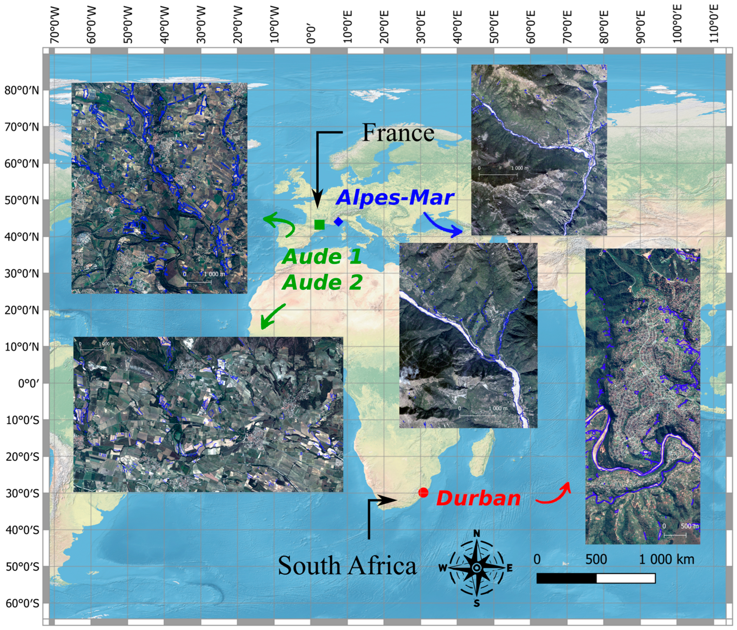
2.1. Study Areas

Four extreme weather events over three study areas were investigated in this paper. All of them were characterized by heavy precipitations within short time periods (1 or 2 days) and featured high intensities (~30 to 40 mm.h⁻¹ and more) resulting in flash flooding. Three of them occurred in the South of France between 2018 and 2020 and were already examined by Cerbelaud et al. [27] using the SPCD method. The fourth event was selected among recent activations of the ICSMD in South Africa to further illustrate the generalizability of the detection method over a completely different landscape. Description and reference for these four events are as follows:

• Aude 1: Intense precipitations affected the Aude French department on 15 October 2018, with close to 300 mm of rainfall measured around the city of Carcassonne within a day. Up to 250 mm fell locally in only 6 h in this mostly agricultural region [50];
• Aude 2: A weaker event occurred in the same area on 11 May 2020, with up to 175 mm cumulative rainfall measured in two days around the town of Montolieu [51];
• Alpes-Mar: The “Alex” massive storm hit the Alpes-Maritimes French department on 2 October and 3 October 2020. Around 500 mm of rainfall was recorded at Saint-Martin-Vésubie in only a day, and up to 90 mm in just an hour was recorded at the Coursegoules rainfall station. Countless landslides and debris flows were reported in this mountainous region [52];
• Durban: Torrential downpours (~300 mm in 24 h) triggered landslides and mudflows on 11 April and 12 April 2022 on the eastern coast of South Africa near Durban in the KwaZulu-Natal province. The death toll in the surrounding areas exceeded 400 [53].

For this work, the areas of interest (AOI) extended over roughly 53 km² for Aude 1, 72 km² for Aude 2, 36 km² for Alpes-Mar (including 20 km² for the Vésubie valley and 16 km² for the Roya) and 31 km² for Durban. Regions were selected based on the availability of VHR images and overall relevance in the occurrence of PFs. All VHR products were acquired in the context of major disaster activations from either the ICSMD or the Copernicus EMS. Aude 1 and Alpes-Mar events were indeed covered by EMS under the activation numbers EMSR324 and EMSR467. However, grading maps distributed within days after the events mostly focused on overflowing streams and mudslides around major rivers, neglecting surface water floods inland where economic stakes were low. In the Durban region, flash floods and resulting landslides were much more thoroughly investigated by ICube-SERTIT through ICSMD charter activation 755. A map describing the precise location of all four study sites is provided in Figure 2.

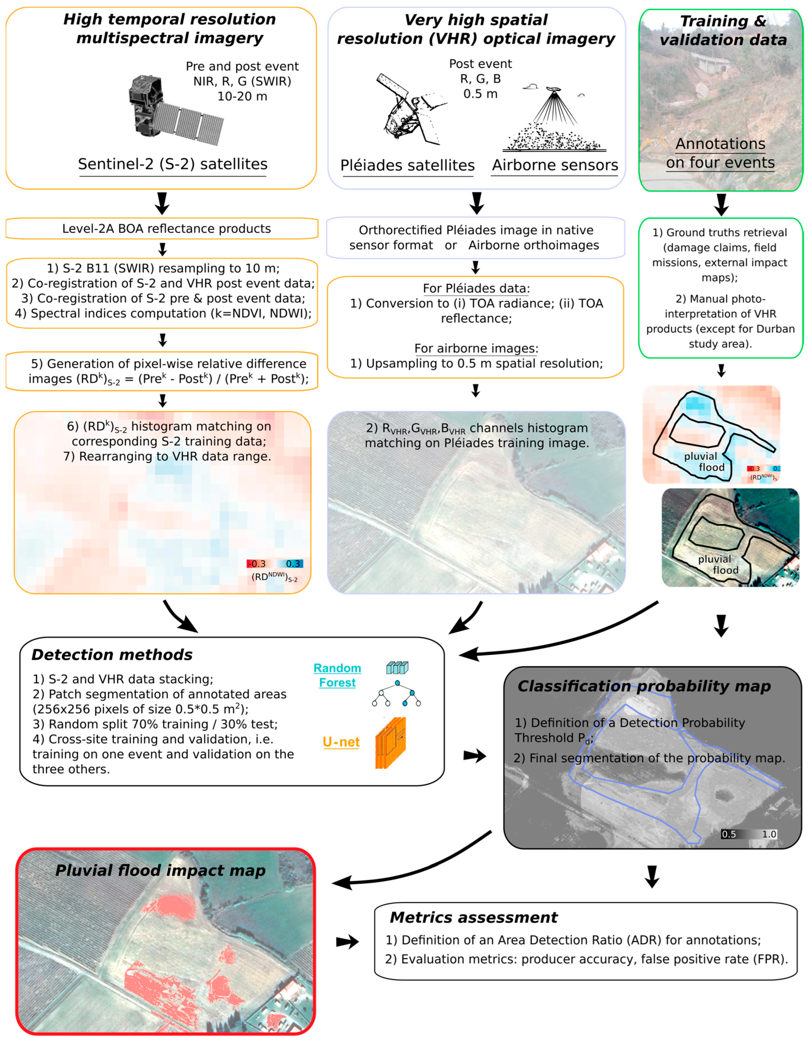
2.2. Remote Sensing Data and Pre-Processing Steps

Building on the works of Cerbelaud et al. [27] in which S-1 and S-2 bi-temporal data were combined to establish the plot-based SPCD method, a new pixel-based approach was developed involving the fusion of S-2 change images with VHR post event imagery (see Figure 1).

2.2.1. Post Event Very High Spatial Resolution (VHR) Products

For this purpose, the earliest available post event VHR Pléiades satellite images were retrieved from ICSMD or EMS activations. The panchromatic spatial resolution of the Pléiades’ optical instrument is 0.7 m, along with four spectral bands in the visible and near-infrared (NIR) ranges at 2.8 m resolution (see

Table 1. Acquisition dates and imaging capabilities of Pléiades, IGN airborne and Sentinel-2 (non-exhaustive) optical instruments.

Satellite or Airborne Product	Acquisition Dates Event X: Date t				Wavelength Range (nm)	Spatial Resolution
	Aude 1: 15 October 2018	Aude 2: 11 May 2020	Alpes-Mar: 3 October 2020	Durban: 12 April 2022
Pléiades TOA reflectance (VHR)	Post event 2018/11/03	Post event 2020/05/22		Post event 2022/04/14	Panchromatic 480–820 Blue (B0) 450–530 Green (B1) 510–590 Red (B2) 620–700 NIR (B3) 775–915	0.7 m (panchromatic) 2.8 m (multispectral) Pan-sharpened to 0.5 m (all bands)
IGN orthophotos (VHR)			Post event Multiple tiles starting 2020/10/05		Visible (blue, green and red)	~0.1 m
Sentinel-2 Level-2A BOA reflectance (High revisit)	Pre event 2018/10/05 (S-2A) Post event 2018/10/25 (S-2A)	Pre event 2020/05/07 (S-2A) Post event 2020/05/20 (S-2A)	Pre event 2020/09/28 (S-2A) Post event 2020/10/08 (S-2A)	Pre event 2022/03/29 (S-2B) Post event 2022/04/28 (S-2B)	Blue (B2) 460–525 Green (B3) 542–578 Red (B4) 650–680 NIR (B8) 780–886 SWIR (B11) 1565–1660	10 m for bands B2, B3, B4 and B8 20 m for band B11

for information). Multispectral images are eventually provided at 0.5 m pan-sharpened and resampled spatial resolution with orthorectification and in sensor native basic radiometric format. Digital numbers were then converted to top-of-atmosphere (TOA) radiance using gain and bias values provided with the products and ultimately to TOA reflectance by controlling for band-specific solar irradiance and solar zenith angle at acquisition time. Reflectance indeed provides a standardized measure that is directly comparable between images. There was no need for atmospheric correction here because acquisitions were monotemporal (post event only) and all made in clear sky conditions. TOA reflectance products already bear consistent spectral capability that statistical learning methods can exploit. Together with 6.5 m location accuracy (Circular Error with a confidence level of 90% at nadir), sub-metric spatial resolution of Pléiades allowed for precise identification of multiple types of rainwater runoff deteriorations through photo-interpretation: landslides and mud/debris flows, gullies, erosion, sediment deposit and vegetation uprooting. In order to allow for generalizability of the ML and DL methods (see Section 2.4) between study sites, normalization was performed on all Pléiades images with Aude 1 as reference data. For this, several approaches were tested (unit normal global normalization, by-patch normalization). However, flattening the data was not a viable option as spectral variability was key for detecting land-cover irregularities caused by PFs. Global histogram matching was eventually the only conclusive method (not shown here) through the “match_histograms” function from the exposure module of the scikit-image Python package. It consists of searching (for each color level of a reference image channel) the level in the target image channel for which cumulative distribution functions of the two images equalize. This technique is particularly helpful to balance detector responses depending on illumination or calibration techniques.

For Alpes-Mar, the French National Institute of Geographic and Forest Information (IGN) acquired airborne orthoimages with ~0.1 m spatial resolution and a geometric accuracy ≤1 m. These images were taken only a few days after the “Alex” storm and were thus even more effective for accurate visual interpretation of damages. However, they did not include a NIR channel, thus hindering the generation of vegetation indices. In order to evaluate the capacity of ML/DL classifiers to be trained on Pléiades data and later function with other types of VHR sensors, orthophotos of the Vésubie and Roya valleys were upsampled to 0.5 m spatial resolution and histogram matched with Aude 1 Pléiades’ final processed image. In particular, the three red/green/blue channels of the orthoimages were converted from [0:255] to the targeted reflectance range through simple linear transformation.

Emphasis was particularly placed on assessing whether the FuSVIPR method could be fed with various kinds of VHR visible data though they may originate from different sensors with contrasting wavelength ranges, optics structures, calibrations and radiometric processing techniques. Because most VHR airborne instruments do not include an NIR channel, the NIR band of Pléiades was left out in the training process to ensure transferability to other VHR products (loss in accuracy was assessed beforehand).

2.2.2. Multispectral Optical Change Images

Furthermore, just as in Cerbelaud et al. [27], precise change images were generated for all 4 study events from Sentinel-2’s closest pre-event and post-event satellite data (Table 1). S-2 change information was vital to confirm actual recent modifications induced via intense surface runoff on post event VHR data. Corresponding S-2 tiles for each event were T31TDH for Aude 1 and Aude 2, T32TLP for Alpes-Mar and T36JTN for Durban. Satellite products were retrieved from the French THEIA platform for Aude 1, Aude 2 and Alpes-Mar with level-2A processing [54]. For Durban, level-2A products were later downloaded directly from the Copernicus Open Access Hub. All of them consisted in orthorectified bottom-of-atmosphere (BOA, i.e., corrected for atmospheric effects) flat reflectance data with sub-pixel multispectral registration. They were acquired either from S-2A or S-2B satellites (see Table 1). Pre and post event images were co-registered with post event images as master images using the ENVI^® software. Each resulting pair of S-2 acquisitions presented values of average sum-of-squared intensity differences (SSD) lower than 0.005 on all four study events. Change images simply consisted in pixel-by-pixel relative difference of vegetation-specific indices based on red (B4), green (B3) and NIR (B8) bands of S-2 (see the formula in item 5 in the left boxes of Figure 1). Indeed, field observations have shown that intense overland water flow is essentially characterized by the presence of eroded soils, mud or sediment deposits and deteriorations in the vegetation cover. It can thus be tracked down through vegetation- and water-based spectral variations in time and space. In particular, NDVI [55] and NDWI [56] have proven very relevant in previous works to detect PF-induced deteriorations [27]. The change images will be hereafter referenced to as (RD^k)_S-2, with k representing the corresponding index. With a 12 m location accuracy and a medium spatial resolution of 10 m for visible and NIR channels (Table 1), S-2′s revisit frequency (~5 days) was fundamental to characterize recent land cover changes that could appear ambiguous on post event images. After cubic resampling from 20 m to 10 m, the B11 SWIR band of S-2 was also considered for identification of post PF traces [27,57]. Indeed, it has been shown to be related to soil moisture [58], which is indicative of floods and a known driver of landslide occurrence [59].

Additionally, in order to fuse VHR post event data with S-2 change images for use as predictors in pixel-based classifiers, co-registration between S-2 post event images and VHR images was also performed using the GeFolki software [60] prior to the generation of the S-2 change images. All S-2 final processed change images were also histogram matched with Aude 1 S-2 data for reference using the same Python exposure module as was used for VHR images. (RD^k)_S-2 values (k = NDVI, NDWI and SWIR) were finally re-mapped to the same reflectance interval as Pléiades ([0,1]*10,000 for integer storage) to avoid feeding the U-net with negative values and in order for it to account for all predictors (VHR and S-2 changes) in a rather balanced way.

All products were used (and projected to, if necessary) in the native reference coordinate system of Sentinel images, World Geodetic System (WGS) 84, either Universal Transverse Mercator (UTM) zone 31N for Aude 1 and Aude 2, UTM zone 32N for Alpes-Mar and UTM zone 36S for Durban.

2.3. Ground Truths Reference Data for Training and Validation

Reference data for flood damages were gathered from various field sources and from VHR imagery photo-interpretation. For the Aude 1 event, previous works [32] already assembled a training/validation dataset from geo-referenced agricultural disaster claims at the plot scale (more than 300 plots on the official land cadastre, source: Aude’s Direction Départementale des Territoires et de la Mer, i.e., DDTM 11). In Cerbelaud et al. [27], information on closed-off road segments was used for Aude 2 (around 180 plots, source: DDTM 11), and field mission ground truths (observations of shallow landslides and debris flows) were acquired for Alpes-Mar (435 plots in the Tinée, Vésubie and Roya valleys). From these affected plots, vector-based annotations were performed manually on VHR post event images to assemble a training/validation dataset. In the Durban case, no photo-interpretation was carried out. The vector impact map resulting from the semi-automatic detection of floods and landslides achieved by ICube-SERTIT for Charter Call 868 (ID 755) was downloaded and directly used as ground truths (Durban Pinetown West, https://sertit.unistra.fr/en/rms/?action=748&product=01 (accessed on 21 April 2023)) even with no guarantee that the inventory was exhaustive. All vectors (polygon shapes) were eventually converted to 0.5 m raster format (=1 for annotated damages, 0 otherwise) for training and/or validation of the FuSVIPR method. Examples of tagged observations from all four events can be seen in Figure 3.

The number and total area of PF annotated shapes are also displayed in Figure 3: 460 shapes for Aude 1, 223 for Aude 2, 205 for Alpes-Mar and 127 for Durban. A great effort to tag deteriorations as exhaustively as possible was made over the entire extent of VHR images (except for Durban) in order to compute false-positive rates on the overall remaining areas. Because this study is entirely focused on PFs, FF-related damages were not accounted for (though they were recorded). Annotated shapes undeniably corresponding to river overflowing were thus removed from damage detection accuracy assessment. However, false-positive rates were computed outside of all types of flood damages, FFs and PFs (see Section 2.5 for details about validation metrics).

2.4. FuSVIPR: Application and Comparison of Two Concurrent Detection Algorithms for PFs

Two supervised learning pixel-based approaches were tested for the FuSVIPR method (Figure 1): (i) the Random Forest (RF) ML classifier and (ii) the U-net CNN DL method for image segmentation. On the one hand, RF has been proven to be highly effective for many classification tasks, it works on any kind of tabular data, is less computationally expensive and does not require as much data to train. CNNs, on the other hand, have been shown to outperform a number of ML algorithms in image segmentation even with small amounts of training data and can still work quite quickly once properly trained.

The two classifiers exposed here were set to perform a binary classification wherein the output was simply a probability map for the detection of a PF-related deterioration. Hence, in this work, the developed classifiers were not designed to distinguish the different types of deteriorations associated with intense overland flow (landslides, mud deposits, debris flows, eroded soils, gullies, etc.) in a multi-class framework. They only indicated the presence or absence of one of these PF-induced damages.

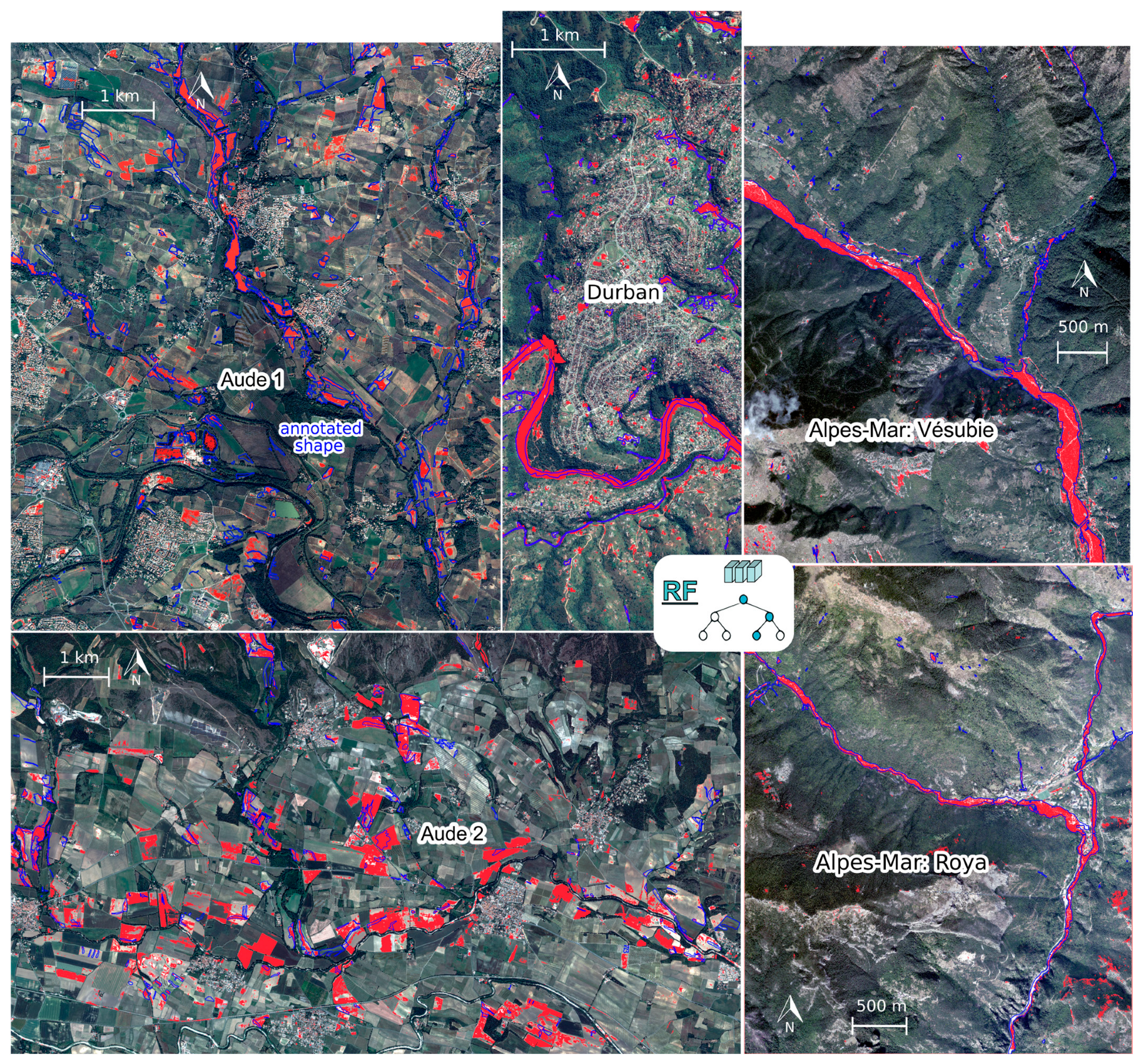
2.4.1. Random Forest (RF)

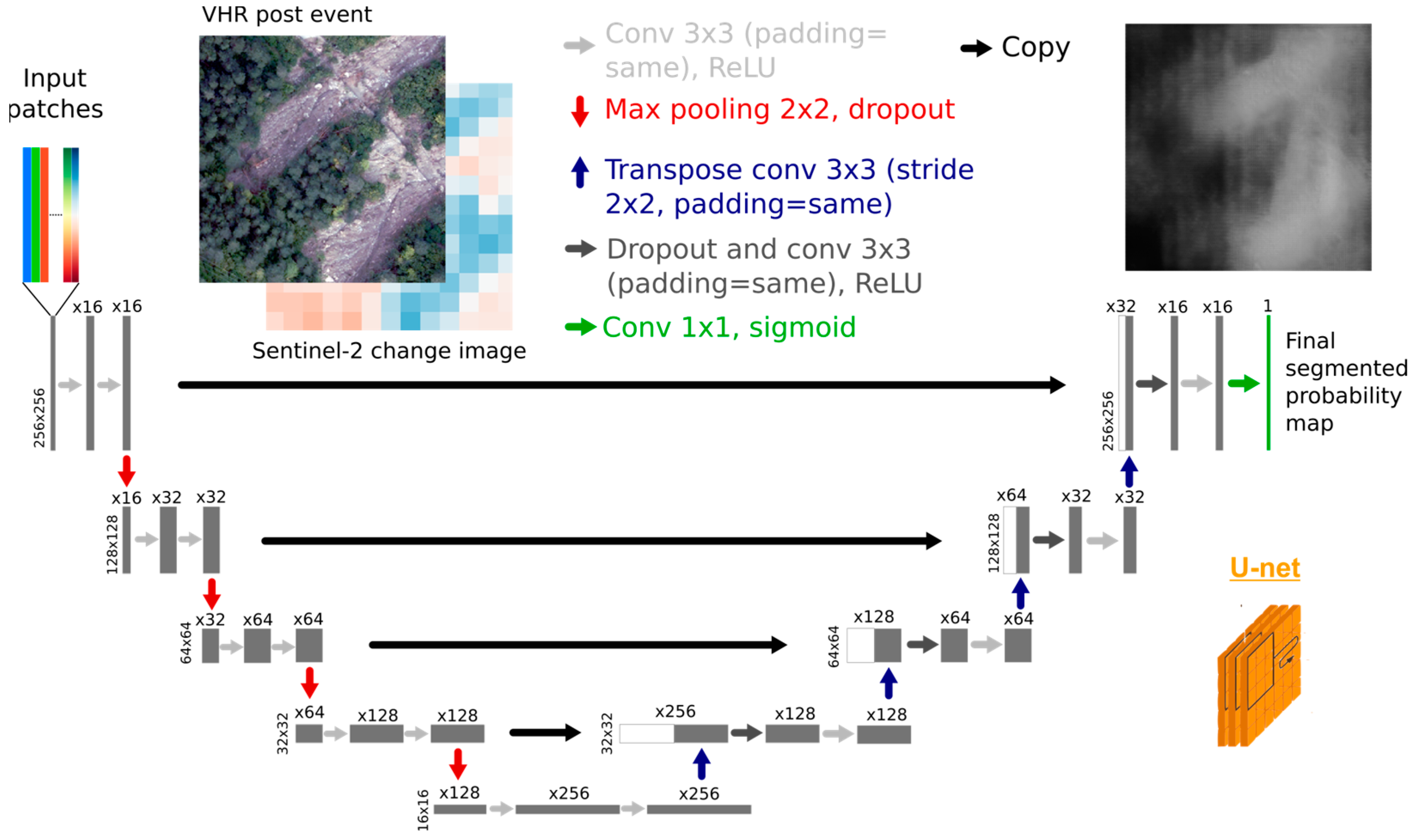
The RF algorithm is a machine learning method used for the classification or regression of tabular data. For classification, it is based on majority voting from a collection of decision trees [61]. Trees are fitted using subsets of training samples to control for overfitting. The core method was first proposed by Ho [49]. Here, the tabular data comprising the pool of predictors for the classification consisted in the spectral characteristics of each 0.25 m² pixel derived from both the VHR post event visible bands (Red, Green and Blue, referenced as R_VHR, G_VHR and B_VHR) and the S-2 change images ((RD^NDVI)_S-2, (RD^NDWI)_S-2 and (RD^SWIR)_S-2).

The 460, 223 and 205 annotated shapes in Aude 1, Aude 2 and Alpes-Mar, respectively, led to a breakdown in images with 800, 513 and 414 patches (256 × 256 pixels of size 0.25 m²), with each patch containing at least one annotation, for learning/validation purposes. This segmentation of images in patches was required for the application of the U-net approach (see Section 2.4.2) and was kept as the basis for RF as well. The learning and validation phases for RF made use of 10⁶ pixels (size determined empirically to limit computational time while reaching good sample representability) selected equally among the N training/test patches for each study event. Hence, 10⁶/N pixels were selected randomly in each patch, half of them within annotations for the “damaged” class, the other half in the rest of the patch for the “non affected” class. These balanced samples of pixels were then randomly split, with 70% data used for training and 30% for testing.

Prior testing was carried out to tune the two hyperparameters of the RF algorithm in order to avoid overfitting (increase in training score but decrease in test score) and unnecessary computational time. Eventually, the maximum depth of trees was set to 10, and the number of trees was set to 5 (see justification in Figure 4). Such a small number of trees proved that the choice of predictors was highly relevant, as opposed to many studies wherein hundreds or even thousands of trees need to be set for RF classification. As shown in Pelletier et al. [62], the gain in overall accuracy with more trees and/or higher depth is often weak in remote sensing classification (a few %) compared to the increase in the computational cost.

Finally, a minimum size threshold segmentation was added as post processing on the output probability maps to better control for false alarms in the detection of PF-type objects (only in RF, not for U-net). Hence, every cluster containing fewer than 200 pixels (optimal size of 50 m²—i.e., half a S-2 pixel—, not shown here) classified as “damaged” by the RF algorithm was considered a noisy, small object and removed. This type of post processing for pixel-based tabular data classification is well known to avoid outliers in image segmentation (e.g., [63]). However, this could also imply the removal of linear shapes such as is found in road damages, which was detrimental to the identification of some PF-related damages.

2.4.2. U-Net

U-net is a type of DL method based on convolutional neural networks. The common framework is comprised of a contracting path and an expansive path, thus taking the shape of a U (Figure 5). It was initially designed for medical imagery segmentation [45]. In recent years, U-nets have become massively used for diverse segmentation applications in remote sensing. Here, a standard architecture was adapted from the literature and tested. Fed with reference semantic data, it iteratively learns the band pattern, shape and content of each desired class within a given set of images in order to later be able to easily classify others.

Predictors at the pixel level were exactly the same as in the RF algorithm, i.e., VHR post event visible bands (R_VHR, G_VHR and B_VHR) and Sentinel-2 change image indices ((RD^NDVI)_S-2, (RD^NDWI)_S-2 and (RD^SWIR)_S-2). Starting from a given initial number of input bands over 256 × 256 pixel patches, the following pattern was repeated four times: (i) two 3 × 3 convolutions with conservation of dimensions (“padding = same”), each followed by a rectified linear unit (ReLU); (ii) a 2 × 2 max pooling operation leading to a halving of dimensions followed by a dropout (p = 0.1, i.e., each neuron has a 10% chance of being deactivated) to control for overfitting. The final dimension of outputs in the contracting path was thus 16 × 16 pixels. The number of filters (i.e., the number of channels, or feature maps, in the outputs) was initially set to 16 for the first two convolutions. It was then multiplied by 2 at each of the three other steps. A fifth and final convolutional block without max pooling/dropout enabled a number of 256 channels to be reached before starting the upsampling path (bottom of Figure 5). The purpose of this contracting path is to capture as much information as possible in the input image to perform the most accurate segmentation.

In the expansive pathway, a “reverse” pattern was iterated four times: (i) a transpose (or up) convolution with a stride of 2 leading to a doubling of dimensions; (ii) a concatenation with the corresponding feature map from the contracting path; (iii) a dropout (p = 0.1 as well) and two 3 × 3 convolutions with conservation of dimensions (“padding = same”), each followed by a rectified linear unit (ReLU). At each step, the number of channels obtained from the transposed convolution and from the following two convolutions is divided by two (thus starting at 128) in order to progressively recover the initial number of 16 filters. Lastly, a 1 × 1 convolution layer is applied with one filter and a sigmoid activation function to produce the final output segmented probability map.

The same 800, 513 and 414 patches (256 × 256 pixels of size 0.25 m²) for Aude 1, Aude 2 and Alpes-Mar containing the annotated shapes were used for learning purposes. These samples were then randomly split, just as for the RF method, with 70% of patches used for training and 30% used for testing. The number of epochs was limited to 50 for each training run. The batch size, i.e., the number of randomly chosen patches used for each iteration inside an epoch, was set to 32 for Aude 1 and 16 for Aude 2 and Alpes-Mar. Data augmentation was implemented on all training patches at each iteration with horizontal flips, width and height shifts and zooms and rotations. Such a process enables the creation of “new” images at each iteration run so as to prevent excessive fitting to the original training data. The optimizer was the Adam algorithm (a stochastic gradient descent method), and cross-entropy was chosen as the loss function between true labels and predicted labels. Design and implementations were carried out under Python 3 using TensorFlow and Keras.

2.5. Validation Approach and Metrics

Evaluation metrics were computed based on detection probability thresholds (P_d) and Area Detection Ratios (ADR, see Figure 6). Indeed, there was first a need to define a probability level on RF and U-net output probability maps from which pixels could be considered affected by a PF, or “damaged”. Then, a classical naive approach would have consisted in using pixel-wise validation metrics. For both RF and U-net methods, overall accuracies (OAs), precision (user accuracy) and recall (producer accuracy) were systematically provided on the test samples following learning runs. However, in our case, as the purpose of the approach was to identify runoff-related impacts, which are represented in an image as a cluster of pixels, an ADR was also defined. The ADR basically represents the minimum percentage of pixels within an annotated damage shape that needs to be classified as damaged (a pixel is classified as “damaged” when its probability P is greater than P_d) for the entire shape to be considered detected. Indeed, man-made annotations are sometimes inaccurate and even frequently erroneous at the boundaries. There was thus no need for part of the pixels inside some shapes to be correctly classified.

False-positive rates (FPRs) were computed from the final classification maps as the ratio of pixels with probability P ≥ P_d among all pixels standing outside 25 m buffers around the annotated damages (optimal buffer size, not shown here). Such buffer was implemented to account for imprecise annotations by avoiding counting pixels above P_d that stood slightly outside annotated shapes as false positives. As a great effort was made to reference all the deteriorations in the study events, the FPRs were calculated over the entire areas excluding annotated floods (and not only over a few selected unaffected areas). Despite all efforts, the annotations were however never completely exhaustive. It is thus very important to mention that all FPRs given here consist in upper bound values. Indeed, some PFs may have been absent from the ground truth sources or may have been missed during the photo-interpretation process. Yet, they can still end up rightfully flagged by the detection method, resulting in an incorrect addition to the FPR (see Section 4.1 for more details). The incomprehensiveness of observational data is an inevitable limitation found in many remote sensing classification studies, which has to be acknowledged. It is not detrimental to the training/test process nor to the validation metrics, as long as the number of untagged reference areas is limited in the training/test patches.

ADR-based detection rates and above-mentioned FPRs were thus chosen as more appropriate for interpretation purposes in this work instead of the pixel-based OA, precision, recall and F1-score commonly used in classification studies. These ad hoc metrics indeed contributed to setting more stringent detection probability thresholds so that false positives could be as infrequent as possible while still accounting for satisfactory detection capacity when PF-induced damages were not necessarily entirely flagged (see Figure 6).

Once again, damages induced by river overflowing were not accounted for in this study. Annotated shapes undeniably corresponding to FFs were thus removed from accuracy assessment. However, FPRs were computed based on the % of pixels featuring a probability of “damage” P ≥ P_d outside all recorded flood damages, i.e., both FFs and PFs.

3. Results

3.1. Detection Probability Threshold (P_d) and Area Detection Ratio (ADR)

In this section, both the RF and U-net classifiers were trained only on the Aude 1 learning sample (800 patches). This dataset was first used as reference for training because it has the highest number of annotated shapes and the most trustworthy sources of PFs (agricultural damage claims from regional authorities).

Detection rates were computed depending on different values for P_d and ADR and are provided on all annotated shapes of each case study. Results related to Aude 2 and Alpes-Mar bore significant values to showcase the method’s generalizability as the classifiers were not trained on these events. Alpes-Mar’s performance was even more meaningful as IGN airborne orthophotos (instead of Pléiades images) acted as VHR data to test the usability of the method on other types of VHR images.

PF-induced damage detection capacity is illustrated in Figure 7 using the red, green and blue channels of the VHR products, i.e., R_VHR, G_VHR and B_VHR, and both (RD^NDVI)_S-2 and (RD^NDWI)_S-2 as predictors (no SWIR). The goal of Figure 7 was not to illustrate final detection capacity nor to thoroughly compare the two methods, but rather to enable the tuning of values for P_d and ADR in order to obtain the best configuration to identify PFs with minimal false positives.

With PF detection rates around 0.90/0.75/0.55 with a 5%/25%/50% ADR and FPRs below 5%, the 0.75 probability threshold P_d seemed like a good compromise for the RF classifier on all three events (black contour bubbles, Figure 7a). Indeed, P_d = 0.85 provided detection rates that were too low (~0.40 and less for 25% ADR), and P_d = 0.65 led to FPRs that were too high to be acceptable (~7% and more). The U-net performed less in this configuration. With P_d = 0.35, for instance, lower detection rates were met for ADR < 50%, yet with similar FPRs for Aude 1 and Aude 2. For Alpes-Mar, the U-net was particularly unsuccessful regardless of the P_d (Figure 7b). This could be explained in two ways. First, Aude 1 annotated shapes (the training data) usually concerned large agricultural damages, whereas Alpes-Mar annotated PF damages had smaller sizes on average. As a convolution-based method, the U-net was not trained to capture some of the scales of changes observed in Alpes-Mar, even with data augmentation. Secondly, similar to what was observed in Cerbelaud et al. [27], S-2 spectral variability was higher in Aude 1 with multiple types of land coverage compared to Alpes-Mar, which featured mostly forest, grasslands and mineral surfaces. Even after histogram matching, spectral signatures might not be sufficiently similar between the two datasets. However, good results from the RF algorithm on Alpes-Mar essentially ruled out this second explanation. As with the SPCD method [27], greater uncertainty in change detection was also observed over the spring season landscape, with Aude 2′s FPR being the largest based on the RF classifier (5.2% against 2.6% for Aude 1 and 1.3% for Alpes-Mar, see

Table 2. Detection rates and FPR results, depending on the use of S-2 change image predictors. Detection is given on all annotated shapes, depending on ADR (25%-5%). False-positive rates outline the entire remaining areas outside damage buffers. OA, precision and recall in the first column are computed on the Aude 1 test patches, which represent 30% of the overall annotated patches.

Models Are Trained Only on Aude 1	RVHR, GVHR and BVHR + (RDk)S-2 Indices/Bands k Used for S-2	OA-Precision-Recall On Test Patches Aude 1 At Pixel Level	Aude 1		Aude 2		Alpes-Mar
			Detection Rates with ADR 25%-5%	FPR	Detection Rates with ADR 25%-5%	FPR	Detection Rates with ADR 25%-5%	FPR
Random Forest (Pd = 0.75)	(a)	84%-49%-32%	48%-77%	5.4%	67%-84%	6.2%	77%-100%	6.6%
	(b) NDVI, NDWI	88%-66%-52%	75%-89%	2.6%	73%-87%	5.2%	79%-93%	1.3%
	(c) I NDVI, NDWI, SWIR	89%-68%-54%	76%-91%	2.4%	72%-88%	5.3%	79%-95%	1.7%
U-net CNN (Pd = 0.35)	(a)	85%-56%-46%	65%-77%	3.9%	65%-86%	15.1%	55%-61%	13.4%
	(b) NDVI, NDWI	87%-59%-56%	67%-77%	2.0%	63%-79%	4.8%	60%-65%	8.8%
	(c) I NDVI, NDWI, SWIR	88%-65%-53%	63%-70%	1.3%	76%-88%	6.8%	57%-61%	2.3%

). With blooming and rapidly developing crops, it is understandably more difficult to distinguish land cover changes in mid-May due to surface runoff from those due to natural evolutions solely from multispectral data.

Setting P_d to 0.75 for RF and 0.35 for U-net, classification performances were then assessed depending on the choice of input predictors. Several forests and networks were trained on Aude 1 data (a) using only VHR visible bands R_VHR, G_VHR and B_VHR; (b) adding (RD^NDVI)_S-2 and (RD^NDWI)_S-2 and (c) adding (RD^NDVI)_S-2, (RD^NDWI)_S-2 and (RD^SWIR)_S-2. The essential role of S-2 change information in conjunction with VHR data was consequently revealed for both detection methods. Full results are displayed in Table 2.

Indeed, when S-2 change information was omitted and only post event VHR data were used for model training (Table 2 row (a)), performances were lower for both methods. In the case of RF, pixel-based Oas computed on the test sample (Aude 1) were only 4 to 5% lower (84% vs. ~88% when S-2 was used), but ADR-based detection rates on all annotated shapes of Aude 1 were much worse (48–77% vs. ~75–90% when S-2 was used), as were FPRs (5.4% vs. ~2.5% when S-2 was used). When transferring the trained RF to the other study cases, detection rates were good, but only because FPRs were too high (e.g., 6.6% vs. ~1.5% for Alpes-Mar when S-2 was used). For U-net, the network obtained through and adjusted to the Aude 1 dataset regardless of the combination of predictors (~65–77% detection rates). However, the CNN trained only on VHR data (Table 2 row (a) for U-net) was not generalizable at all (~15% FPRs in Aude 2 and Alpes-Mar), which pointed to systematic overfitting of the U-net to the Aude 1 training data. Only the addition of S-2 change predictors allowed for good transferability with lower FPRs, but with still rather low detection rates (~60–70% in Table 2 rows (b) and (c) for U-net).

For combinations (b) and (c) in Table 2 (i.e., fusion with S-2 change indices), RF eventually performed better than U-net in terms of ADR-based detection rates (10% to 20% higher) on all study cases with similar FPRs (except on Alpes-Mar, wherein U-net struggled more). Eventually, the addition of SWIR change information did not seem to significantly improve the performance of either RF or U-net. Improved (degraded) detection rates only occurred in conjunction with higher (lower) FPRs. This result was in line with the findings of Cerbelaud et al. [27] from the SPCD method, wherein SWIR did not add significant prediction capability for PF-induced deteriorations when visible/NIR-based indices were already used. Two reasons could explain this inadequacy: (i) the spatial resolution of 20 m for the SWIR bands of S-2 is too coarse or (ii) as S-2 post event images were not acquired soon enough after the floods (i.e., a few days [57]), SWIR spectral signatures could not indicate residual moisture.

This analysis shows that it is important to look at potentially more appropriate metrics and try to transfer classifiers to other case studies. Indeed, if only pixel-based metrics given by the programmed algorithm on the test patches (which were independent from the training one, but still part of the same scene from Aude 1) were considered here, one would not find S-2 to be vital for accurate detection, and U-net would be found to perform equally as RF.

Finally, dropping out the NIR_VHR band of Pléiades images was quantified on Aude events. It resulted in a mean modification of OA, precision, recall, 25% ADR-based detection rate and FPR of, respectively, +1%, +3%, −1%, +2% and −0.1% for U-net in the (b) configuration (i.e., weak modifications). Hence, R_VHR, G_VHR and B_VHR were ruled as sufficient for classification here, confirming that FuSVIPR could also potentially be relevant with other visible-only VHR products.

3.2. Cross Validation Results

Poor results transferring U-net from Aude 1 to Alpes-Mar could stem from differences in the structures and sizes of PF-induced deteriorations between the two areas. Indeed, Alpes-Mar annotations were mostly smaller in size and showed a greater variety in shape. As a strictly pixel-based tabular approach, RF should not be influenced by such contrasts compared to U-net. This was confirmed through the performance of the ML algorithm on Alpes-Mar (Table 2). A cross-site validation approach was thus used as a robustness check and for further comparison of RF and U-net methods in FuSVIPR (

Table 3. Cross-validation results. Detection is given on all annotated shapes depending on ADR (25%-5%). False-positive rates outline the entire remaining areas outside damage buffers. OA, precision and recall in the first column are computed on the test patches (from the same site as training), which represent 30% of the overall annotated patches.

RVHR, GVHR, BVHR + (RDNDVI)S-2, (RDNDWI)S-2	Training Site	OA-Precision-Recall On Test Patches Same Site as Training At Pixel Level	Aude 1		Aude 2		Alpes-Mar
			Detection Rates with ADR 25%-5%	FPR	Detection Rates with ADR 25%-5%	FPR	Detection Rates with ADR 25%-5%	FPR
Random Forest	Aude 1 (Pd = 0.75) 460 shapes 800 patches	88%-66%-52%	75%-89%	2.6%	73%-87%	5.2%	79%-93%	1.3%
	Aude 2 (Pd = 0.70) 223 shapes/513 patches	82%-42%-54%	62%-87%	2.9%	76%-91%	4.3%	56%-96%	1.8%
	Alpes-Mar (Pd = 0.70) 205 shapes/414 patches	94%-79%-89%	66%-87%	2.6%	62%-80%	4.1%	91%-98%	1.4%
U-net CNN	Aude 1 (Pd = 0.35) 460 shapes/800 patches	87%-59%-56%	67%-77%	2.0%	63%-79%	4.8%	60%-65%	8.8%
	Aude 2 (Pd = 0.20) 223 shapes/513 patches	76%-35%-67%	73%-91%	5.7%	82%-91%	6.5%	35%-67%	1.0%
	Alpes-Mar (Pd = 0.10) 205 shapes/414 patches	85%-53%-94%	66%-77%	1.9%	64%-79%	5.3%	77%-88%	2.0%

). The 5-predictor combination (Table 2, row (b)) was finally chosen: R_VHR, G_VHR, B_VHR, (RD^NDVI)_S-2 and (RD^NDWI)_S-2.

With different training data, additional tests (comparable to those displayed in Figure 7) were performed to set the optimal values of the detection probability threshold P_d. Obviously, the best results were obtained for each study event when training was conducted on the site itself (diagonals in Table 3). Better Oas on test samples were obtained with RF compared to U-net, in line with RF’s overall better behavior concerning detecting damages with reasonable ADR and low FPR. Aude 2 trained classifiers yielded the worst results, echoing previous findings on the complexity of the spectral and spatial data for this event. FPRs on that same event were still rather high for both RF and U-net. On the contrary, with the Alpes-Mar training dataset, outstanding results were obtained on Alpes-Mar (which was to be expected), but also on the two other study cases. Looking at U-net, the CNN performed on Aude 1 and Aude 2 similarly to when Aude 1 was used for training. Hence, training the U-net on Alpes-Mar wherein annotated shapes were smaller in size enabled better identification of damages in this same site while still performing well on the Aude events. Hence, when using U-net for object identification, one should rather train on smaller-sized annotations for better transferability to larger ones, not the opposite. For RF, much less difference in performance was observed between Aude 1 and Alpes-Mar training, as expected from the architecture of the method.

Final optimal results for RF (Aude 1 training) and U-net (Alpes-Mar training) are displayed in

Table 4. Final performance (detection rates and FPRs) for all four study events.

RVHR, GVHR, BVHR + (RDNDVI)S-2, (RDNDWI)S-2	OA-Precision-Recall On Test Patches Same Site as Training At Pixel Level	Aude 1		Aude 2		Alpes-Mar		Durban
		Detection Rates with ADR 25%-5%	FPR	Detection Rates with ADR 25%-5%	FPR	Detection Rates with ADR 25%-5%	FPR	Detection Rates with ADR 25%-5%	FPR
RF * Aude 1 training (Pd = 0.75)	88%-66%-52%	75%-85%	1.9%	73%-86%	4.9%	77%-86%	0.6%	70%-91%	1.2%
U-net Alpes-Mar training (Pd = 0.10)	85%-53%-94%	66%-77%	1.9%	64%-79%	5.3%	77%-88%	2.0%	77%-92%	1.8%

* After minimum-size-threshold segmentation.

after post processing according to minimum size threshold segmentation to remove small noisy objects (only in RF, which does not have a convolution-based structure). Additional validation was finally conducted on the Durban case study. Similar performances were reached with FPRs below 2% and 70–91% (77–92%) of photo-interpreted shapes (with 25%-5% ADR) correctly detected by RF (respectively, U-net) from the landslide impact map produced by Icube-SERTIT. This result additionally proved the operational potential of FuSVIPR to automatically provide future impact maps of PFs without requiring further training. Moreover, this exhibits fine capacity to derive damage maps in lightly populated periurban areas where interpretation of remote sensing images still poses major challenges. Optimal detection capacity of FuSVIPR is illustrated with close-up examples in Figure 8, in the video provided as part of the Supplementary Data and over all the study sites in Figure 9.

4. Discussion

4.1. Detection Extent and False Alarms

In order to further discuss the detection capacity of both classifiers in the FuSVIPR method, the distributions of ADRs among all annotated shapes in the final detection maps (metrics exposed in Table 4) are displayed in the violin plots in Figure 10.

In the RF case, half of all annotated shapes were detected with an ADR greater or equal to 53%, 66%, 45% and 35% (=ADR_med) in Aude 1, Aude 2, Alpes-Mar and Durban, respectively. Looking at the first quartile of ADR, 75% of ground truths were detected with an ADR of at least 24%, 20%, 26% and 15% in the study events. The two classifiers can easily be distinguished. For U-net, median ADRs were higher, and overall distributions were more dichotomous (Figure 10b). Indeed, the CNN-based method mostly either recognized the shapes (with ADR ≥ 60%) or did very little (ADR < 10%). For the RF approach, the distribution was much more scattered, with shapes being detected at various ADRs. This main difference was the result of RF being a pixel-based tabular approach as opposed to U-net operating with convolution layers that are meant to recognize overall shapes and structures. For Aude 1, Aude 2 and Alpes-Mar, the bottom bump in the distributions corresponded to ~0% ADR for RF and even more so for U-net, meaning that a certain number of shapes were not seen at all with the two methods. In the Durban case, SERTIT annotations were detected with smaller ADRs globally (larger bumps in the bottom of the distribution), but a non-negligible number of shapes were still detected at the bottom of the distribution (for instance, at around 12% ADR in the RF case). Distribution statistics revealed that U-net seemed like the most appropriate method for Durban if one was looking for higher average ADRs with still reasonably low FPRs (<2%). RF, on the other hand, allowed for better identification of PFs on the other study sites, even if only smaller portions were tagged on average. Section 4.3 provides some additional insights on the violin plots displayed in Figure 10.

As already mentioned, PF damage annotations can never be completely thorough (which is one of the reasons why FuSVIPR was developed). This had no effect on the PF detection rates as they were calculated on the basis of producer accuracies (also called recall, i.e., how many ground truths were positively detected). However, as FPRs were computed over the overall remaining areas (i.e., how many pixels were classified as “damaged” everywhere outside annotations), it is important to insist that all FPRs given in this work constitute maximum values. Indeed, some areas that were missed during the photo-interpretation process were sometimes rightfully detected with the method (see Figure 11), inducing spurious rises in the FPR. This also demonstrates the performance of the FuSVIPR method to automatically identify relevant PF-induced damages that operators can miss while photo-interpreting post event imagery. Either way, FPRs below 2% were found in all study events, except in Aude 2 (<5%, Table 4). Such accuracy is mostly unprecedented in the detection of post-flood traces of intense pluvial runoff, especially with supervised classifiers that were not trained on parts of the reference data. Indeed, Cerbelaud et al. [27] reached optimal FPRs of 10% in Aude study sites using the SPCD method, and those were computed on a limited number of photo-interpreted unaffected plots only, not on the overall remaining unaffected areas.

4.2. Comparison with the SPCD Method from Cerbelaud et al. [27] and Other Related Approaches

Final performances from either ML or DL classifiers roughly exceeded 75% detection rates with 25% ADR in conjunction with low FPRs (<2% mostly) for all four study events. By comparison, Dhakal et al. [29] reached 88% OA using Landsat TM data (which have 30 m resolution, i.e., not VHR) to identify flash flood damages, but only on one study area in Nepal and with limited annotated ground truths (<50).

Using an object-based support vector machine (SVM) landslide classifier on a GeoEye-1 multispectral image, Heleno et al. [30] obtained 95% producer accuracy and a false-discovery rate below 26% in Madeira Island, but once again with no transferability assessment to other areas/events. With U-net and ResU-net DL networks, Ghorbanzadeh et al. [38] implemented an S-2-based landslide detection method and reached precisions mostly under 70%. However, they tested their networks on three different areas of interest with cross-validation and site-specific training datasets as well. Interestingly, they found no improved generalized performance when collectively merging all their case studies into one global training dataset. Meena et al. [39] compared several ML methods to U-net for landslide inventory using Rapid-Eye satellite imagery (5 m resolution) and found U-net performed slightly better with precisions around 70% as well. Cerbelaud et al. [27] evaluated the SPCD repeatable method on extended datasets of Aude 1, Aude 2 and Alpes-Mar events with S-2 change images (no VHR data) and found similar accuracies at plot scale, but with globally higher FPRs (see

Table 5. Comparative performances of the FuSVIPR and SPCD [27] methods regarding pluvial floods.

Pluvial Flood Deteriorations Types of Detection Method	Method’s Characteristics	Aude 1		Aude 2		Alpes-Mar
		Detection Rates	FPR	Detection Rates	FPR	Detection Rates	FPR
FuSVIPR-RF Aude 1 trained (Pd = 0.75)	(i) Pixel-based (ii) VHR + S-2 (iii) 0.5 m resolution (iv) U-net or RF	75%-85% (ADR 25%-5%)	2%	73%-86%	5%	77%-86%	1%
SPCD Aude 1 trained (Pd = 0.50, Table 5a from [27])	(i) Plot-based (ii) S-2 (+S-1) + land cadastre + land cover (iii) 10 m resolution (iv) GP classifier	84% (at plot level)	12%	74%	4%	70%	1%

for a comparison between SPCD and FuSVIPR). They also showed that their method was quite robust regarding the use of distant S-2 images, should stable ground conditions be observed before the event. With a 30-day interval between the two Durban images (the largest gap in our four study sites, see Table 1) because of persistent cloud cover, FuSVIPR was also proven in this study to be able to work well with moderately distant S-2 images. All things considered, SPCD is an easy, fast and large-scale method for broad mapping of PFs (and FFs, for that matter) when only S-2 open-source images are available. However, SPCD does not provide the exact location of deteriorations within the detected plots and is not meant to work in periurban or urban areas. When a VHR post event product is available (≤0.5 m here), FuSVIPR enables actual detection of PF shapes at a finer resolution and potentially allows for complex damage identifications in lightly populated areas (Figure 8 and Figure 9).

The PF damage detection rates reached with FuSVIPR (~75%) turned out to be lower than what other related studies on flood damages and rainfall-induced landslides have found (~85% to 90%, [29,30]). This, however, has to be alleviated, considering that our results are valid with four different events with a classifier trained on only one of the events. Indeed, most classification methods featuring higher detection rates (85% and more) are usually tested on the same event (and thus the same remote sensing images) that they were trained on. In particular, for instance, the SPCD method had also been found to reach up to 90% detection rates when trained and validated on only one event [32] before these accuracies were updated and lowered to ~70% after performing a transferability assessment over two additional events [27].

4.3. Random Forest Classifier or U-Net Semantic Segmentation?

FuSVIPR was developed to function with two famous methods for classification of remote sensing images. If training was significantly longer for U-net (~2.5 h for 800 256 × 256 patches and 50 epochs on a 16 GB 11th Gen. Intel Core i7 @ 3.00 GHz processor, vs. a few seconds for RF), both are fast when applied on large-scale VHR data and S-2 change images (a few minutes) once trained and provide accurate pattern detection of PF-induced damages (Table 4).

In the literature, Du et al. [64] found that, for dynamic classification of paddy rice, U-nets outperformed RF when relying solely on pixel-based OA and F1-Score for their unique case study test sample. Yoo et al. [65] compared CNN to RF for local climate zone (LCZ) classification using bi-temporal Landsat 8 data of four urban areas with a transferability assessment study. By training the model on three cities and evaluating the results on the remaining one, they concluded that the DL classifier systematically resulted in 7–18% higher OAs. In two subtropical forest fragments of Southern Brazil, tree species were classified using hyperspectral data from unmanned aerial vehicles, with the CNN approach being 22–26% more accurate than the SVM and RF [66]. ML methods were faster but less stable to changes in datasets and depended on prior segmentation and hand-engineered features to reach similar accuracies to those of the CNN. In other works related to earth observation and geosciences, Taghizadeh-Mehrjardi et al. [67] analyzed the spatial distribution of soil particle size fractions (PSF) in digital soil mapping. They found that CNN consistently outperformed RF with, for example, around 20% lower RMSE values for clay, sand, and silt contents at the top layer when using CNN compared to RF. In our study, pixel-based OA, precision and recall displayed in Table 4 did not unequivocally show that U-net outperformed RF. However, globally, U-net better mapped the full extent of damages, as shown in the violin plots in Figure 10. Yet, when considering an ADR approach (i.e., detecting only certain parts of the damages), RF demonstrated a better capacity to detect at least small portions of some shapes that U-net did not see at all. This is very consistent with the works of Ge et al. [68], who already determined for transferability of crop mapping that U-net performed better overall, while RF was better in target areas where plots were smaller. In addition, here, FPRs were systematically lower in the RF case after minimum size thresholding. A noteworthy observation is that in the Durban additional validation case, the DL method performed better at detecting a greater portion of the extent of annotated shapes while not missing as much damages as in the other study events (no bottom bump in the distribution) and featuring similar FPR compared with RF. For instance, 50% ADR corresponded roughly to the 4th decile for U-net, while it was above the third quartile for RF (Figure 10). This meant that roughly 60% of all shapes were at least half detected with U-net, compared to only around 20% for RF. In addition, RF tended to wrongly tag complex building structures, on occasion, in the Durban case (Figure 12). U-net globally appeared to be the best method to deal with lightly populated urban areas, wherein interpretation of patterns among complex landscapes is even more crucial.

Overall, if many research activities recently stated the superiority of U-net for segmentation tasks over ML techniques such as RF, our study does not unquestionably conclude in the same direction. Both methods can indeed provide good detection capacity, depending on user-defined objectives such as computational cost and speed, comprehensive segmentation, irregular pattern recognition or false-alarm minimization.

5. Conclusions

Pluvial or surface water floods have been estimated as being accountable for half of all flood damage claims in the past years, equally with fluvial floods. With the expected intensification of regional extreme short-duration precipitation events in the coming years, flash floods are highly likely to escalate further. Comprehensive detection of runoff-related impacts following heavy weather events is therefore critical to allow for thorough evaluation and improvement of PF susceptibility mapping models. With ground truths being very hard to collect and rarely exhaustive, remote sensing stands as a very promising tool to specifically identify pluvial flood footprints on the ground after extreme rainfall events. In this context, a novel automatic remote sensing method called FuSVIPR for Fusion of Sentinel-2 & Very high resolution Imagery for Pluvial Runoff was developed. Making the most of some of the best spatial resolution (0.5 m) and freely accessible frequent revisit (5 days) today in satellite optical imagery, FuSVIPR can generate unprecedented large-scale pixel-based observational data on pluvial floods with satisfactory detection rates (~75%) and low false positive rates (mostly < 2%). Its major contribution lies in the great transferability of the trained U-net and Random Forest classifiers, which was displayed across four diversified events and landscapes, making FuSVIPR potentially operational in various regions and all year round. Both classifiers presented good detection capacity, and neither of them stood out as the best one. RF is recommended for more comprehensive segmentation, especially for small, isolated deteriorations, but U-net does a better job dealing with complex shapes in periurban landscapes. Further tests should be carried out to confirm high generalizability in other environments. Once two cloudless and closely timed Sentinel-2 images are retrievable before and after a flood event, the FuSVIPR method can be applied with different types of VHR post event visible data, i.e., from satellites, airborne sensors or even probably UAVs (unmanned Aerial Vehicles). Final segmented maps of PF-induced damages provide valuable, reliable and unbiased observational data for evaluation and improvement of intense surface runoff susceptibility models at very high spatial resolution. Applications to natural hazard mapping in alpine environments for instance could also be conceived for the study of mountain torrents and rapid mass movements. Furthermore, this method shows great potential for helping extreme precipitation downscaling from radar ground measurements using stochastic simulators or geostatistical techniques such as kriging through informing on the distribution of PF-affected areas in similar ways rain gauge networks inform on local precipitation.

References

1. IPCC. 2022: Summary for Policymakers. In Climate Change 2022: Impacts, Adaptation and Vulnerability; Contribution of Working Group II to the Sixth Assessment Report of the Intergovernmental Panel on Climate Change; Pörtner, H.-O., Roberts, D.C., Tignor, M., Poloczanska, E.S., Mintenbeck, K., Alegría, A., Craig, M., Langsdorf, S., Löschke, S., Möller, V., et al., Eds.; Cambridge University Press: Cambridge, UK; New York, NY, USA, 2022; pp. 3–33. [Google Scholar] [CrossRef]
2. Jenkins, K.; Surminski, S.; Hall, J.; Crick, F. Assessing surface water flood risk and management strategies under future climate change: Insights from an Agent-Based Model. Sci. Total Environ. 2017, 595, 159–168. [Google Scholar] [CrossRef]
3. Ebi, K.L.; Vanos, J.; Baldwin, J.W.; Bell, J.E.; Hondula, D.M.; Errett, N.A.; Hayes, K.; Reid, C.E.; Saha, S.; Spector, J.; et al. Extreme Weather and Climate Change: Population Health and Health System Implications. Annu. Rev. Public Health 2021, 42, 293–315. [Google Scholar] [CrossRef]
4. Gudmundsson, L.; Boulange, J.; Do, H.X.; Gosling, S.N.; Grillakis, M.G.; Koutroulis, A.G.; Leonard, M.; Liu, J.; Schmied, H.M.; Papadimitriou, L.; et al. Globally observed trends in mean and extreme river flow attributed to climate change. Science 2021, 371, 1159–1162. [Google Scholar] [CrossRef] [PubMed]
5. Fowler, H.J.; Ali, H.; Allan, R.P.; Ban, N.; Barbero, R.; Berg, P.; Blenkinsop, S.; Cabi, N.S.; Chan, S.; Dale, M.; et al. Towards advancing scientific knowledge of climate change impacts on short-duration rainfall extremes. Phil. Trans. R. Soc. A 2021, 379, 20190542. [Google Scholar] [CrossRef] [PubMed]
6. Cerbelaud, A.; Breil, P.; Blanchet, G.; Roupioz, L.; Briottet, X. Proxy data of surface water floods in rural areas: Application to the evaluation of the IRIP intense runoff mapping method based on satellite remote sensing and rainfall radar. Water 2022, 14, 393. [Google Scholar] [CrossRef]
7. Moncoulon, D.; Labat, D.; Ardon, J.; Leblois, E.; Onfroy, T.; Poulard, C.; Aji, S.; Rémy, A.; Quantin, A. Analysis of the French insurance market exposure to floods: A stochastic model combining river overflow and surface runoff. Nat. Hazards Earth Syst. Sci. 2014, 14, 2469–2485. [Google Scholar] [CrossRef]
8. Bernet, D.B.; Prasuhn, V.; Weingartner, R. Surface water floods in Switzerland: What insurance claim records tell us about the damage in space and time. Nat. Hazards Earth Syst. Sci. 2017, 17, 1659–1682. [Google Scholar] [CrossRef]
9. Speight, L.J.; Cranston, M.D.; White, C.J.; Kelly, L. Operational and emerging capabilities for surface water flood forecasting. WIREs Water 2021, 8, e1517. [Google Scholar] [CrossRef]
10. Li, C.; Handwerger, A.L.; Wang, J.; Yu, W.; Li, X.; Finnegan, N.J.; Xie, Y.; Buscarnera, G.; Horton, D.E. Augmentation of WRF-Hydro to simulate overland-flow- and streamflow-generated debris flow susceptibility in burn scars. Nat. Hazards Earth Syst. Sci. 2022, 22, 2317–2345. [Google Scholar] [CrossRef]
11. Dehotin, J.; Breil, P. Technical Report of the IRIP Project: Surface Runoff Flood Hazard Mapping; Technical Report; IRSTEA Hydrology-Hydraulic Research Unit: Lyon, France, 2011. [Google Scholar]
12. Kim, J.-C.; Lee, S.; Jung, H.-S.; Lee, S. Landslide susceptibility mapping using random forest and boosted tree models in Pyeong-Chang, Korea. Geocarto Int. 2018, 33, 1000–1015. [Google Scholar] [CrossRef]
13. Costache, R.; Barbulescu, A.; Pham, Q.B. Integrated Framework for Detecting the Areas Prone to Flooding Generated by Flash-Floods in Small River Catchments. Water 2021, 13, 758. [Google Scholar] [CrossRef]
14. Costache, R.; Tin, T.T.; Arabameri, A.; Crăciun, A.; Ajin, R.S.; Costache, I.; Islam, A.R.; Abba, S.I.; Sahana, M.; Avand, M.; et al. Flash-flood hazard using deep learning based on H2O R package and fuzzy-multicriteria decision-making analysis. J. Hydrol. 2022, 609, 127747. [Google Scholar] [CrossRef]
15. Ouma, Y.O.; Lottering, L.; Tateishi, R. Soil Erosion Susceptibility Prediction in Railway Corridors Using RUSLE, Soil Degradation Index and the New Normalized Difference Railway Erosivity Index (NDReLI). Remote Sens. 2022, 14, 348. [Google Scholar] [CrossRef]
16. Gatto, M.P.A.; Montrasio, L. X-SLIP: A SLIP-based multi-approach algorithm to predict the spatial–temporal triggering of rainfall-induced shallow landslides over large areas. Comput. Geotech. 2023, 105175. [Google Scholar] [CrossRef]
17. Salvatici, T.; Tofani, V.; Rossi, G.; D’Ambrosio, M.; Tacconi Stefanelli, C.; Masi, E.B.; Rosi, A.; Pazzi, V.; Vannocci, P.; Petrolo, M.; et al. Application of a physically based model to forecast shallow landslides at a regional scale. Nat. Hazards Earth Syst. Sci. 2018, 18, 1919–1935. [Google Scholar] [CrossRef]
18. Yu, D.; Coulthard, T.J. Evaluating the importance of catchment hydrological parameters for urban surface water flood modelling using a simple hydro-inundation model. J. Hydrol. 2015, 524, 385–400. [Google Scholar] [CrossRef]
19. Rahman, M.S.; Di, L. The state of the art of spaceborne remote sensing in flood management. Nat. Hazards 2017, 85, 1223–1248. [Google Scholar] [CrossRef]
20. Munawar, H.S.; Hammad, A.W.A.; Waller, S.T. Remote Sensing Methods for Flood Prediction: A Review. Sensors 2022, 22, 960. [Google Scholar] [CrossRef] [PubMed]
21. Byun, Y.; Han, Y.; Chae, T. Image Fusion-Based Change Detection for Flood Extent Extraction Using Bi-Temporal Very High-Resolution Satellite Images. Remote Sens. 2015, 7, 10347–10363. [Google Scholar] [CrossRef]
22. Li, Y.; Martinis, S.; Wieland, M. Urban flood mapping with an active self-learning convolutional neural network based on TerraSAR-X intensity and interferometric coherence. ISPRS J. Photogramm. Remote Sens. 2019, 152, 178–191. [Google Scholar] [CrossRef]
23. Goffi, A.; Stroppiana, D.; Brivio, P.A.; Bordogna, G.; Boschetti, M. Towards an automated approach to map flooded areas from Sentinel-2 MSI data and soft integration of water spectral features. Int. J. Appl. Earth Obs. Geoinf. 2020, 84, 101951. [Google Scholar] [CrossRef]
24. Kocaman, S.; Tavus, B.; Nefeslioglu, H.A.; Karakas, G.; Gokceoglu, C. Evaluation of Floods and Landslides Triggered by a Meteorological Catastrophe (Ordu, Turkey, August 2018) Using Optical and Radar Data. Geofluids 2020, 8830661, 18. [Google Scholar] [CrossRef]
25. Shahabi, H.; Shirzadi, A.; Ghaderi, K.; Omidvar, E.; Al-Ansari, N.; Clague, J.J.; Geertsema, M.; Khosravi, K.; Amini, A.; Bahrami, S.; et al. Flood Detection and Susceptibility Mapping Using Sentinel-1 Remote Sensing Data and a Machine Learning Approach: Hybrid Intelligence of Bagging Ensemble Based on K-Nearest Neighbor Classifier. Remote Sens. 2020, 12, 266. [Google Scholar] [CrossRef]
26. Tavus, B.; Kocaman, S.; Gokceoglu, C. Flood damage assessment with Sentinel-1 and Sentinel-2 data after Sardoba dam break with GLCM features and Random Forest method. Sci. Total Environ. 2022, 816, 151585. [Google Scholar] [CrossRef]
27. Cerbelaud, A.; Roupioz, L.; Blanchet, G.; Breil, P.; Briottet, X. A repeatable change detection approach to map extreme storm-related damages caused by intense surface runoff based on optical and SAR remote sensing: Evidence from three case studies in the South of France. ISPRS J. Photogramm. Remote Sens. 2021, 182, 153–175. [Google Scholar] [CrossRef]
28. Cerbelaud, A.; Favro, A.; Roupioz, L.; Blanchet, G.; Briottet, X.; Delvit, J.-M.; Breil, P. Potential of high resolution satellite optical imagery to detect damages following extreme rainfall events. La Houille Blanche 2020, 6, 66–74. [Google Scholar] [CrossRef]
29. Dhakal, A.S.; Amada, T.; Aniya, M.; Sharma, R.R. Detection of areas associated with flood and erosion caused by a heavy rainfall using multitemporal Landsat TM data. Photogramm. Eng. Remote Sens. 2002, 68, 233–239. [Google Scholar]
30. Heleno, S.; Matias, M.; Pina, P.; Sousa, A.J. Semiautomated object-based classification of rain-induced landslides with VHR multispectral images on Madeira Island. Nat. Hazards Earth Syst. Sci. 2016, 16, 1035–1048. [Google Scholar] [CrossRef]
31. Yokoya, N.; Yamanoi, K.; He, W.; Baier, G.; Adriano, B.; Miura, H.; Oishi, S. Breaking Limits of Remote Sensing by Deep Learning from Simulated Data for Flood and Debris-Flow Mapping. IEEE Trans. Geosci. Remote Sens. 2020, 60, 4400115. [Google Scholar] [CrossRef]
32. Cerbelaud, A.; Roupioz, L.; Blanchet, G.; Breil, P.; Briottet, X. Supervised classification methods for automatic damage detection caused by heavy rainfall using multitemporal high resolution optical imagery and auxiliary data. Int. Arch. Photogramm. Remote Sens. Spat. Inf. Sci. 2021, XLIII-B3-2021, 693–700. [Google Scholar] [CrossRef]
33. Proy, C.; Tinel, C.; Fontannaz, D. Pleiades in the context of the International Charter “Space and Major Disasters”. In Proceedings of the 2013 IEEE International Geoscience and Remote Sensing Symposium—IGARSS, Melbourne, VIC, Australia, 21–26 July 2013; pp. 4530–4533. [Google Scholar] [CrossRef]
34. Yésou, H.; Chastanet, P.; Maxant, J.; Huber, C.; Clandillon, S.; Battiston, S.; Proy, C.; de Fraipont, P. Contribution de l’imagerie Pléiades à la cartographie rapide des dégâts suite à des catastrophes majeures: Retours d’expériences après deux ans d’actions de cartographie rapide localisées en Asie, en Afrique, en Europe et aux Caraïbes. Rev. Fr. Photogramm. Télédétection 2015, 209, 81–87. [Google Scholar] [CrossRef]
35. Yésou, H.; Escudier, A.; Battiston, S.; Dardillac, J.-Y.; Clandillon, S.; Uribe, C.; Caspard, M.; Giraud, H.; Maxant, J.; Durand, A.; et al. Exploitation de l’imagerie Pléiades-THR en cartographie réactive suite à des catastrophes naturelles ayant affecté le territoire français en 2013. Rev. Fr. Photogramm. Télédétection 2015, 209, 39–45. [Google Scholar] [CrossRef]
36. Chen, A.; Darbon, J.; De Franchis, C.; Facciolo, G.; Meinhardt, E.; Michel, J.; Morel, J.-M. Numerical simulation of landscape evolution and water runoff on digital elevation models obtained from Pleiades. Rev. Fr. Photogramm. Télédétection 2015, 209, 117–123. [Google Scholar] [CrossRef]
37. Huang, F.; Chen, L.; Yin, K.; Huang, J.; Gui, L. Object-oriented change detection and damage assessment using high-resolution remote sensing images, Tangjiao Landslide, Three Gorges Reservoir, China. Environ. Earth Sci. 2018, 77, 183. [Google Scholar] [CrossRef]
38. Ghorbanzadeh, O.; Crivellari, A.; Ghamisi, P.; Shahabi, H.; Blaschke, T. A comprehensive transferability evaluation of U-Net and ResU-Net for landslide detection from Sentinel-2 data (case study areas from Taiwan, China, and Japan). Sci. Rep. 2021, 11, 14629. [Google Scholar] [CrossRef] [PubMed]
39. Meena, S.R.; Soares, L.P.; Grohmann, C.H.; van Westen, C.; Bhuyan, K.; Singh, R.P.; Floris, M.; Catani, F. Landslide detection in the Himalayas using machine learning algorithms and U-Net. Landslides 2022, 19, 1209–1229. [Google Scholar] [CrossRef]
40. Saha, S.; Bovolo, F.; Bruzzone, L. Unsupervised Deep Change Vector Analysis for Multiple-Change Detection in VHR Images. IEEE Trans. Geosci. Remote Sens. 2019, 57, 3677–3693. [Google Scholar] [CrossRef]
41. Zhang, C.; Wei, S.; Ji, S.; Lu, M. Detecting Large-Scale Urban Land Cover Changes from Very High Resolution Remote Sensing Images Using CNN-Based Classification. ISPRS Int. J. Geo-Inf. 2019, 8, 189. [Google Scholar] [CrossRef]
42. Peng, X.; Zhong, R.; Li, Z.; Li, Q. Optical Remote Sensing Image Change Detection Based on Attention Mechanism and Image Difference. IEEE Trans. Geosci. Remote Sens. 2021, 59, 7296–7307. [Google Scholar] [CrossRef]
43. Sun, S.; Mu, L.; Wang, L.; Liu, P. L-UNet: An LSTM Network for Remote Sensing Image Change Detection. IEEE Geosci. Remote Sens. Lett. 2022, 19, 8004505. [Google Scholar] [CrossRef]
44. Chen, H.; Qi, Z.; Shi, Z. Remote Sensing Image Change Detection with Transformers. IEEE Trans. Geosci. Remote Sens. 2022, 60, 5607514. [Google Scholar] [CrossRef]
45. Ronneberger, O.; Fischer, P.; Brox, T. U-Net: Convolutional Networks for Biomedical Image Segmentation. In Medical Image Computing and Computer-Assisted Intervention—MICCAI 2015. MICCAI 2015. Lecture Notes in Computer Science; Navab, N., Hornegger, J., Wells, W., Frangi, A., Eds.; Springer: Cham, Switzerland, 2015; Volume 9351. [Google Scholar] [CrossRef]
46. Brand, A.K.; Manandhar, A. Semantic segmentation of burned areas in satellite images using a U-net-based convolutional neural network. Int. Arch. Photogramm. Remote Sens. Spat. Inf. Sci. 2021, XLIII-B3-2021, 47–53. [Google Scholar] [CrossRef]
47. Basnyat, B.; Roy, N.; Gangopadhyay, A. Flood Detection using Semantic Segmentation and Multimodal Data Fusion. In Proceedings of the 2021 IEEE International Conference on Pervasive Computing and Communications Workshops and other Affiliated Events, Kassel, Germany, 22–26 March 2021; pp. 135–140. [Google Scholar] [CrossRef]
48. Feng, Y.; Sester, M. Extraction of Pluvial Flood Relevant Volunteered Geographic Information (VGI) by Deep Learning from User Generated Texts and Photos. ISPRS Int. J. Geo Inf. 2018, 7, 39. [Google Scholar] [CrossRef]
49. Ho, T.K. Random Decision Forest. In Proceedings of the 3rd International Conference on Document Analysis and Recognition 1995, Montreal, QC, Canada, 14–16 August 1995; pp. 278–282. [Google Scholar]
50. Lebouc, L.; Payrastre, O.; Bourgin, F. Reconstitution des Débits de Pointe des Crues du 15 Octobre 2018 Dans le Bassin de L'Aude. Convention DGPR-IFSTTAR 2018 n° 2201132931 du 22 mai 2018—Action 7 Appui au SCHAPI; Rapport de Recherche; IFSTTAR: Versailles, France, 2019; 14p. [Google Scholar]
51. Météo-France. Available online: http://pluiesextremes.meteo.fr/france-metropole/Fortes-pluies-sur-le-sud-de-la-France (accessed on 21 April 2023).
52. Carrega, P.; Michelot, N. Une catastrophe hors norme d'origine météorologique le 2 octobre 2020 dans les montagnes des Alpes-Maritimes. Physio Géo 2021, 16, 1–70. [Google Scholar] [CrossRef]
53. Pinto, I.; Zachariah, M.; Wolski, P.; Landman, S.; Phakula, V.; Maluleke, W.; Bopape, M.-J.; Engelbrecht, C.; Jack, C.; McClure, A.; et al. Climate Change Exacerbated Rainfall Causing Devastating Flooding in Eastern South Africa. World Weather Attribution Science Report. 2022. Available online: https://www.worldweatherattribution.org/wp-content/uploads/WWA-KZN-floods-scientific-report.pdf (accessed on 21 April 2023).
54. Hagolle, O.; Huc, M.; Descardins, C.; Auer, S.; Richter, R. MAJA Algorithm Theoretical Basis Document; CERN: Meyrin, Switzerland, 2017. [Google Scholar] [CrossRef]
55. Tucker, C.J. Red and photographic infrared linear combinations for monitoring vegetation. Remote Sens. Environ. 1979, 8, 127–150. [Google Scholar] [CrossRef]
56. McFeeters, S.K. The use of the Normalized Difference Water Index (NDWI) in the delineation of open water features. Int. J. Remote Sens. 1996, 17, 1425–1432. [Google Scholar] [CrossRef]
57. Yésou, H.; Clandillon, S.; Allenbach, B.; Bestault, C.; de Fraipont, P.; Inglada, J.; Favard, J.C. A constellation of advantages with SPOT SWIR and VHR SPOT 5 data for flood extent mapping during the September 2002 Gard event (France). In Proceedings of the IGARSS 2003 IEEE International Geoscience and Remote Sensing Symposium, (IEEE Cat. No.03CH37477), Toulouse, France, 21–25 July 2003; pp. 567–569. [Google Scholar] [CrossRef]
58. Gao, B.C. NDWI—A normalized difference water index for remote sensing of vegetation liquid water from space. Remote Sens. Environ. 1996, 58, 257–266. [Google Scholar] [CrossRef]
59. Wicki, A.; Lehmann, P.; Hauck, C.; Seneviratne, S.I.; Waldner, P.; Stähli, M. Assessing the potential of soil moisture measurements for regional landslide early warning. Landslides 2020, 17, 1881–1896. [Google Scholar] [CrossRef]
60. Brigot, G.; Colin-Koeniguer, E.; Plyer, A.; Janez, F. Adaptation and Evaluation of an Optical Flow Method Applied to Coregistration of Forest Remote Sensing Images. IEEE J. Sel. Top. Appl. Earth Obs. Remote Sens. 2016, 9, 2923–2939. [Google Scholar] [CrossRef]
61. Breiman, L.; Friedman, J.H.; Olshen, R.A.; Stone, C.J. Classification and Regression Trees, 1st ed.; Routledge: Oxfordshire, UK, 1984. [Google Scholar] [CrossRef]
62. Pelletier, C.; Valero, S.; Inglada, J.; Champion, N.; Dedieu, G. Assessing the robustness of Random Forests to map land cover with high resolution satellite image time series over large areas. Remote Sens. Environ. 2016, 187, 156–168. [Google Scholar] [CrossRef]
63. Rüetschi, M.; Small, D.; Waser, L.T. Rapid Detection of Windthrows Using Sentinel-1 C-Band SAR Data. Remote Sens. 2019, 11, 115. [Google Scholar] [CrossRef]
64. Du, M.; Huang, J.; Wei, P.; Yang, L.; Chai, D.; Peng, D.; Sha, J.; Sun, W.; Huang, R. Dynamic Mapping of Paddy Rice Using Multi-Temporal Landsat Data Based on a Deep Semantic Segmentation Model. Agronomy 2022, 12, 1583. [Google Scholar] [CrossRef]
65. Yoo, C.; Han, D.; Im, J.; Bechtel, B. Comparison between convolutional neural networks and random forest for local climate zone classification in mega urban areas using Landsat images. ISPRS J. Photogramm. Remote Sens. 2019, 157, 155–170. [Google Scholar] [CrossRef]
66. Sothe, C.; De Almeida, C.M.; Schimalski, M.B.; La Rosa, L.E.C.; Castro, J.D.B.; Feitosa, R.Q.; Dalponte, M.; Lima, C.L.; Liesenberg, V.; Miyoshi, G.T.; et al. Comparative performance of convolutional neural network, weighted and conventional support vector machine and random forest for classifying tree species using hyperspectral and photogrammetric data. GISci. Remote Sens. 2020, 57, 369–394. [Google Scholar] [CrossRef]
67. Taghizadeh-Mehrjardi, R.; Mahdianpari, M.; Mohammadimanesh, F.; Behrens, T.; Toomanian, N.; Scholten, T.; Schmidt, K. Multi-task convolutional neural networks outperformed random forest for mapping soil particle size fractions in central Iran. Geoderma 2020, 376, 114552. [Google Scholar] [CrossRef]
68. Ge, S.; Zhang, J.; Pan, Y.; Yang, Z.; Zhu, S. Transferable deep learning model based on the phenological matching principle for mapping crop extent. Int. J. Appl. Earth Obs. Geoinf. 2021, 102, 102451. [Google Scholar] [CrossRef]
Figure 1. Methodological workflow of the FuSVIPR method for pluvial flood-induced damage detection.
Remotesensing 15 02361 g001
Figure 2. Regions of interest in the Aude and Alpes-Maritimes departments, France, and in the province of KwaZulu-Natal, South Africa (Natural Earth I shaded relief and water basemap). Post event Pléiades images and IGN orthophotos of the study sites are provided. Ground truths delineation of flood damages (both FFs and PFs) are outlined in blue.
Remotesensing 15 02361 g002
Figure 3. Ground truth sources and photo-interpreted PF-induced damages in the various study events. Information about the total number of annotated shapes is given in the top-right panel. Durban shapes were downloaded from ICube-SERTIT website for Charter Call 868 (ID 755) (https://sertit.unistra.fr/ (accessed on 21 April 2023)).
Remotesensing 15 02361 g003
Figure 4. Training and test scores on Aude 1 sample for different maximum depths of trees (left) and numbers of trees (right) used in the RF algorithm. Setting a number of 5 trees along with a maximum depth of 10 provided a good compromise between performance and computational speed while avoiding overfitting (increasing training score but decreasing test score).
Remotesensing 15 02361 g004
Figure 5. U-net convolutional neural network (CNN) architecture. Grey boxes represent patches of input rasters or processed features. The number of channels and dimensions are indicated above and on the left of each box, respectively. The input patches correspond to 256 × 256 pixels sampled from the VHR post event image bands and Sentinel-2 change image indices. The final output of the CNN consists of a segmented map providing the probability of detecting a damaged pixel. Arrows represent operations as labelled in the legend.
Remotesensing 15 02361 g005
Figure 6. Area Detection Ratio (ADR) as a function of Pd in Alpes-Mar (Roya). Annotations are delineated in blue, and detected pixels are in red (higher probabilities are darker). Here, Pd = 0.75 (bottom left) appears as a good compromise between sufficient detection (70% of the annotated shape is flagged) and a low FPR (~0.05%) in the rest of the patch. Corresponding ADR-based detection rates (up to 70% ratio) then enable consideration of the shape as 100% detected in the evaluation metrics.
Remotesensing 15 02361 g006
Figure 7. PF detection rates as a function of the Area Detection Ratio (ADR) and detection probability threshold (Pd) over Aude 1, Aude 2 and Alpes-Mar. Training was only performed here on Aude 1 data. The sizes of the bubbles correspond to the labels inside them and refer to the detection rates computed on all annotated shapes. Bubble colors refer to the FPR (depending only on Pd). Black contoured bubbles represent good performance compromise with detection rates around 0.75 for a 25% ADR and FPR below 5% (RF case). (a) Random Forest. (b) U-net.
Remotesensing 15 02361 g007
Figure 8. Close-up of FuSVIPR results on all study events using a unique training sample (Aude 1 for RF and Alpes-Mar for U-net) based on 5 predictors: RVHR, GVHR, BVHR, (RDNDVI)S-2 and (RDNDWI)S-2. Overflowing damages are also detected, but were not accounted for in accuracy assessments. Blue lines and red pixels depict the ground truths and PFs detected with FuSVIPR, respectively.
Remotesensing 15 02361 g008
Figure 9. Detection capability of the FuSVIPR method (RF only) on all four study events using a unique training sample from the Aude 1 event based on 5 predictors: RVHR, GVHR, BVHR, (RDNDVI)S-2 and (RDNDWI)S-2. Overflowing damages are also detected, but were not accounted for in accuracy assessments. Blue lines and red pixels depict the ground truths and PFs detected with FuSVIPR, respectively.
Remotesensing 15 02361 g009
Figure 10. Violin plots of ADR for the 460 (Aude 1), 223 (Aude 2), 205 (Alpes-Mar) and 127 (Durban) annotated shapes in the final (a) RF and (b) U-net post-processed detection maps (Table 4). ADRmed and ADR25th correspond to the median and first quartile value of ADR. Violin plots represent the distribution of values among a dataset similarly to boxplots, with the addition of a rotated smoothed density plot on each side of the boxplot.
Remotesensing 15 02361 g010
Figure 11. Illustrations of missing annotated shapes (red ovals in the left images) that were correctly detected using the FuSVIPR method (either U-net or RF in the right images) in Aude 1, Aude 2 and Durban. Such configurations induced spurious rises in the FPRs. Hence, all FPRs given in this study systematically constituted upper limit values. In this figure, blue lines and red pixels depict the ground truths and PFs detected through FuSVIPR, respectively.
Remotesensing 15 02361 g011
Figure 12. Complexity of detection in lightly populated periurban areas in Durban. RF tended to flag many pixel clusters with akin spectral signatures such as buildings and houses, while the convolution-based U-net managed to rule out these specific shapes to only capture part of the landslide. Results here are both based on Aude 1 training for binding comparison (RF and U-net).
Remotesensing 15 02361 g012