
Geospatial Modeling Based-Multi-Criteria Decision-Making for Flash Flood Susceptibility Zonation in an Arid Area


Abstract
:1. Introduction
2. Materials and Methods
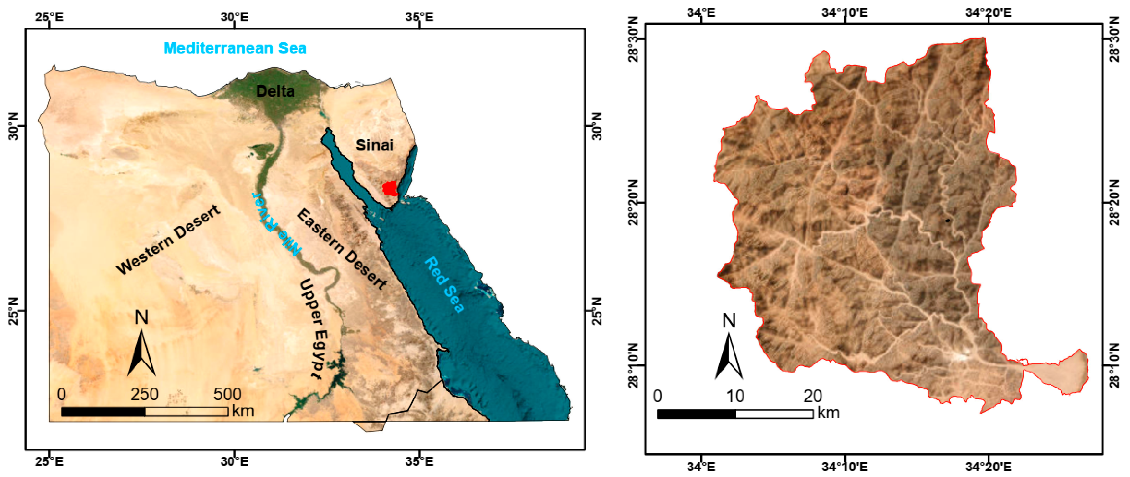
2.1. Area of Study
2.2. Data
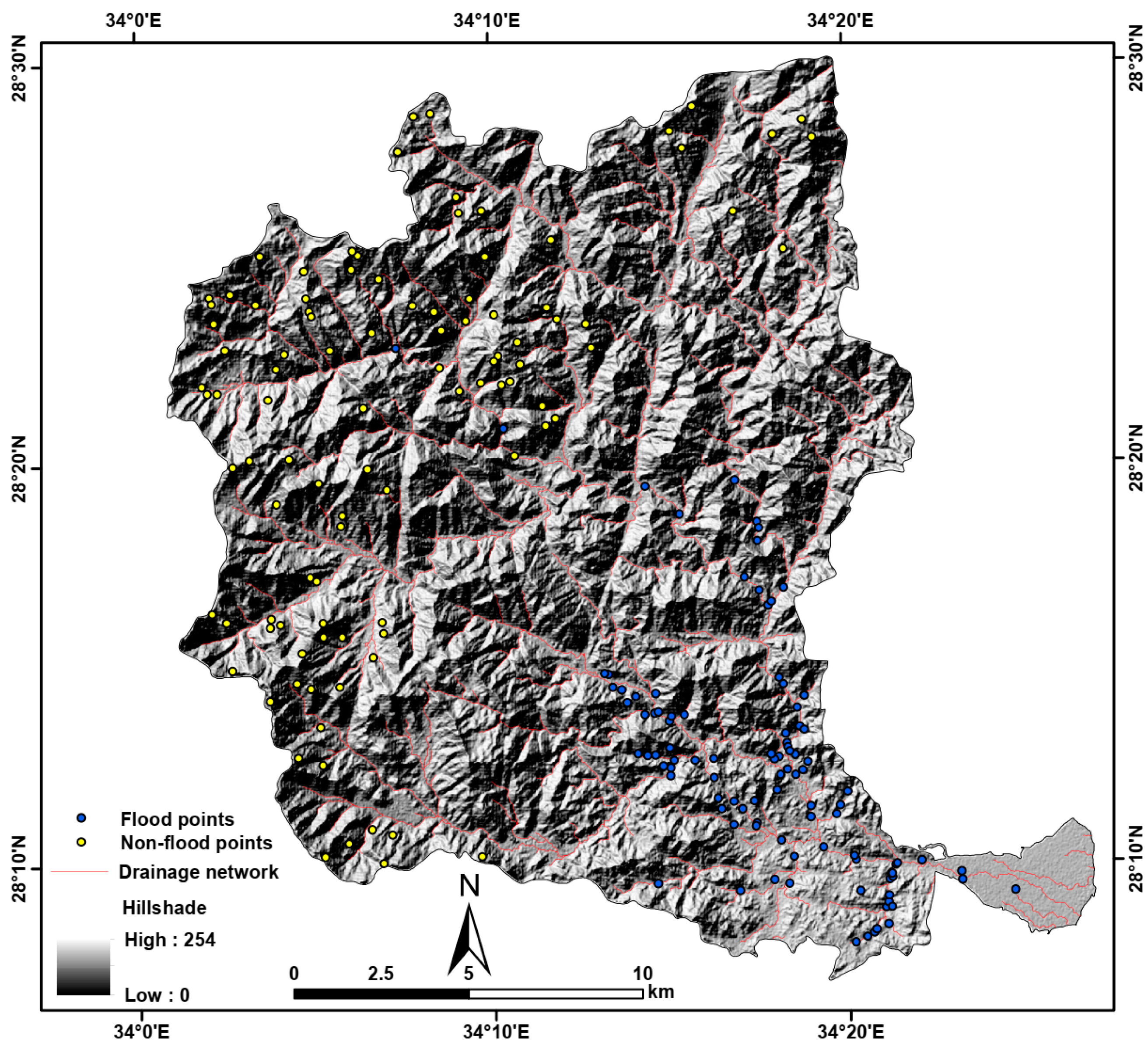
2.2.1. Flash Flood Inventory Map
2.2.2. Description of the Digital Elevation Model (DEM) Used in the Current Study
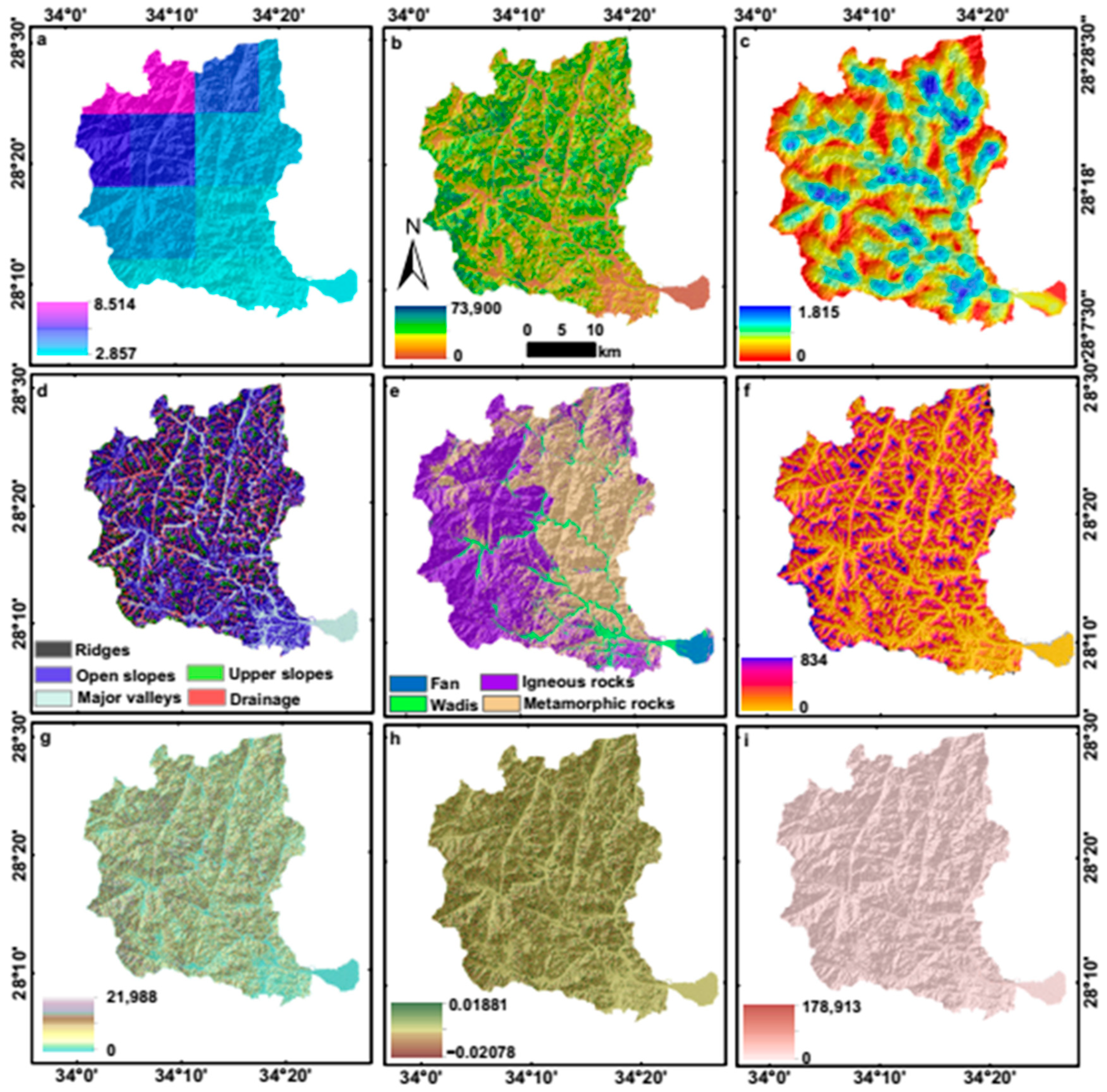
2.2.3. Definition of the Flash Flood Triggering Factors
2.2.4. Preparation of the Satellite Precipitation Data Using NASA Giovanni Web Tool

| Variables’ Definitions | |
|---|---|
| E |
|
| VFD |
|
| HFD |
|
| TWI |
|
| DfW |
|
| FL_UP |
|
| RSP |
|
| CI | |
| PfC |
|
| STI |
|
| Variables’ Definitions | |
|---|---|
| RF |
|
| S |
|
| DD |
|
| LF |
|
| G |
|
| HAND |
|
| MRN |
|
| PnC |
|
| SPI | |
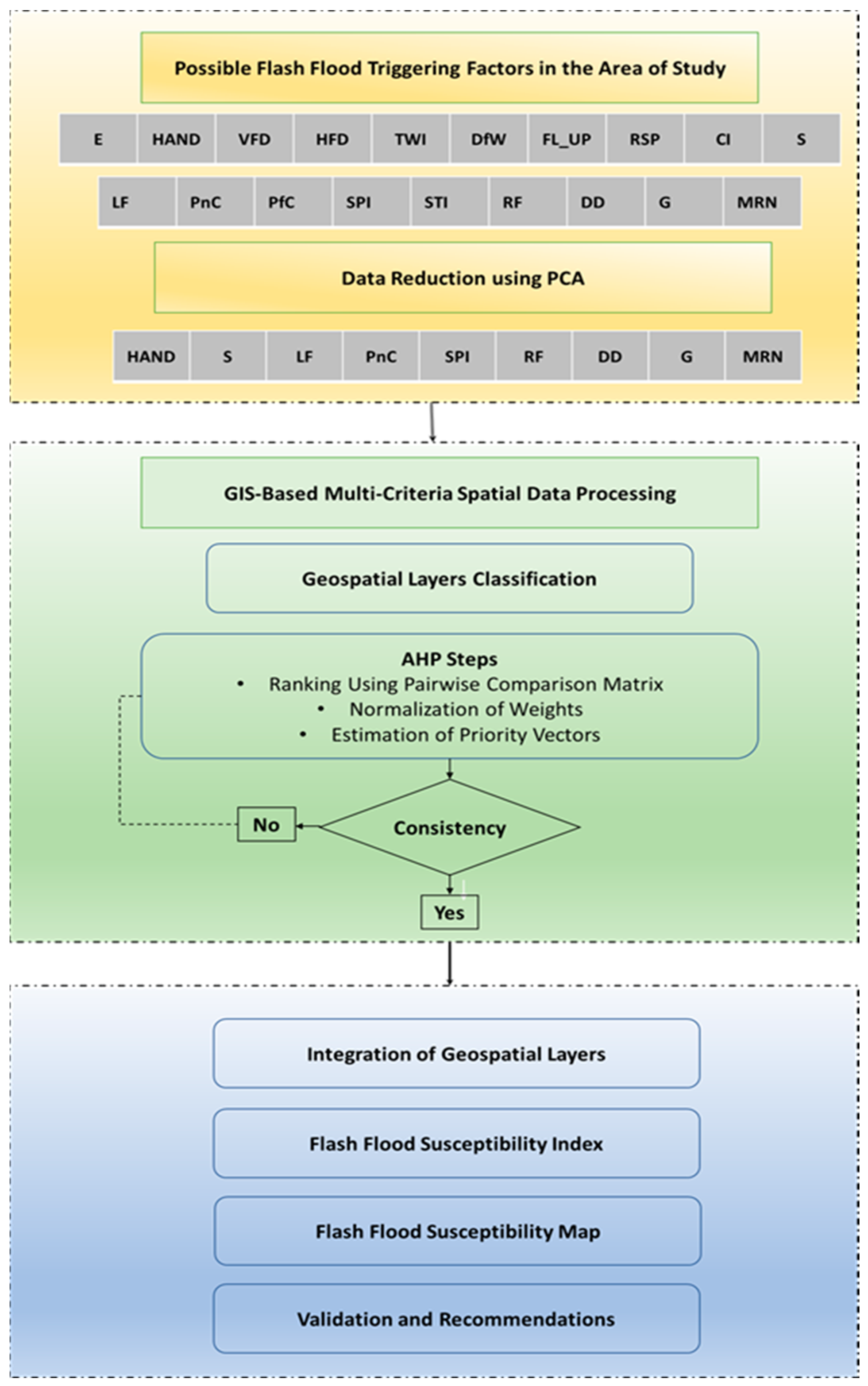
2.3. Methods
2.3.1. Principle Component Analysis (PCA)
2.3.2. Analytical Hierarchy Process (AHP)
2.3.3. Flood Susceptibility Zonation
2.3.4. Accuracy Assessment of the Susceptibility Model
3. Results
3.1. Principal Component Analysis (PCA)
3.2. Assignment of Weight and Rank to Each Flash Flood Triggering Factor
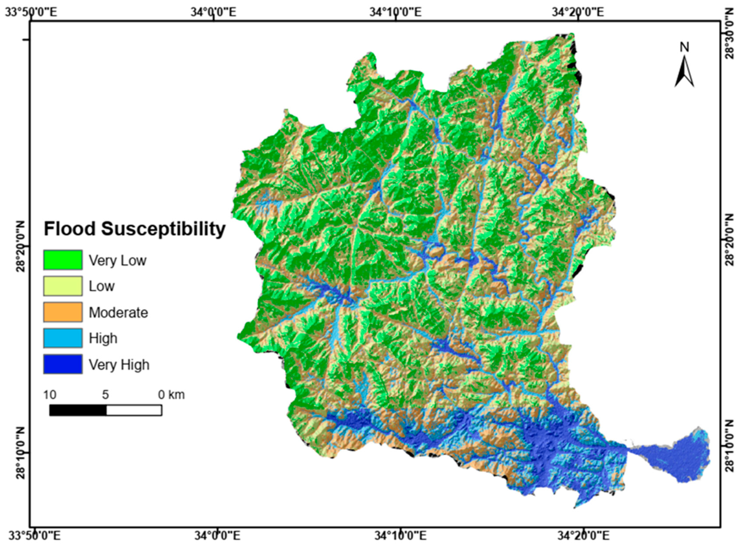
3.3. Mapping of Flash Flood Susceptibility Zonation Using AHP Model Outputs
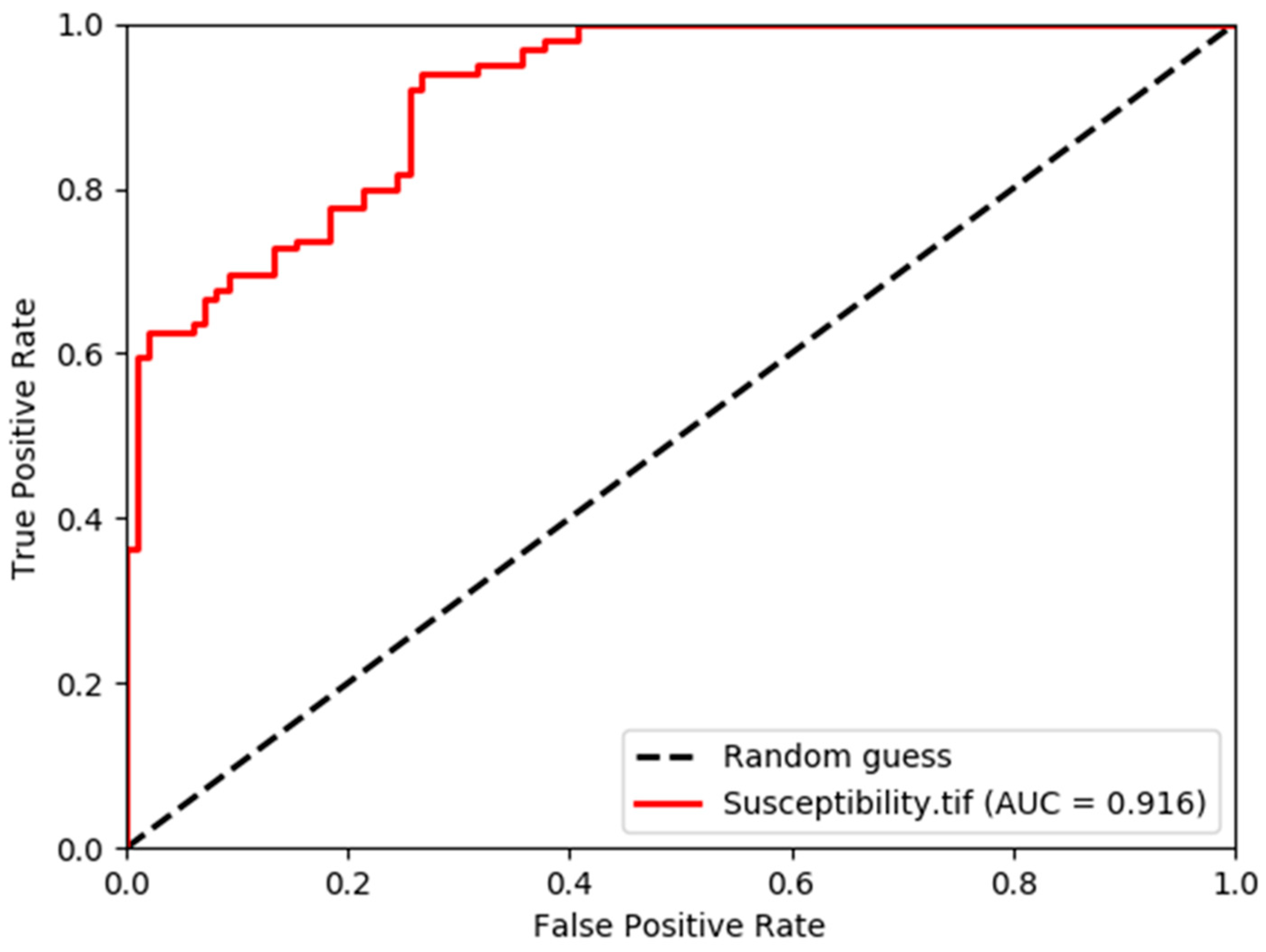
3.4. Accuracy Assessment of the GIS-Based AHP Flash Flood Susceptibility Model
4. Discussion
4.1. Comparison of the Current Findings with the Prior Studies
4.2. Significance of the Selected Flash Flood Triggering Factors in the Current Study
4.3. Pros and Cons of the Developed AHP-Based Flash Flood Susceptibility Model
4.4. Mitigation of Flash Floods’ Impact
4.5. Potential Applications of the Introduced Model
5. Conclusions
Author Contributions
Funding
Data Availability Statement
Acknowledgments
Conflicts of Interest
References
- Wheater, H. Modeling Hydrological Processes in Arid and Semi Arid Areas. Wheater, H. Modelling hydrological processes in arid and semi-arid areas: An introduction. In Hydrological Modelling in Arid and Semi-Arid Areas; Wheater, H., Sorooshian, K., Sharma, K., Eds.; Cambridge University Press: Cambridge, UK, 2007; pp. 1–20. [Google Scholar] [CrossRef]
- Youssef, A.M.; Pradhan, B.; Gaber, A.F.D.; Buchroithner, M.F. Geomorphological Hazard Analysis along the Egyptian Red Sea Coast between Safaga and Quseir. Nat. Hazards Earth Syst. Sci. 2009, 9, 751–766. [Google Scholar] [CrossRef]
- Hong, Y.; Adhikari, P.; Gourley, J.J. Flash Flood. In Encyclopedia of Natural Hazards; Encyclopedia of Earth Sciences Series; Bobrowsky, P.T., Ed.; Springer: Dordrecht, The Netherlands, 2013. [Google Scholar] [CrossRef]
- Borga, M.; Anagnostou, E.N.; Bloschl, G.; Creutin, J.D. Flash Flood Forecasting, Warning and Risk Management: The HYDRATE Project. Environ. Sci. Policy 2011, 14, 834–844. [Google Scholar] [CrossRef]
- Taha, A.H.A.; Ibrahim, E.H.; Shalaby, A.S.; Shawky, M. Evaluation of Geological Hazards for Landuse Planning in Nabq Protectorate, Southeastern Sinai Using GIS Techniques. Int. J. Geosci. 2013, 04, 816–836. [Google Scholar] [CrossRef]
- Schick, A.P.; Grodek, T.; Lekach, J. Sediment Management and Flood Protection of Desert Towns: Effects of Small Catchments. Hum. impact Eros. Sediment. Proc. Int. Symp. Rabat Morocco 1997, 245, 183–189. [Google Scholar]
- Allan, R.P.; Soden, B.J. Atmospheric Warming and the Amplification of Precipitation Extremes. Science 2008, 321, 1481–1484. [Google Scholar] [CrossRef]
- Negm, A.M.; Omran, E.S.E. Introduction to “Flash Floods in Egypt”. In Flash Floods in Egypt; Springer Nature: Cham, Switzerland, 2020; pp. 3–9. [Google Scholar]
- El Zawahry, A.; Soliman, A.H.; Bekhit, H. Critical Analysis and Design Aspects of Flash Flood in Arid Regions: Cases from Egypt and Oman. In Flash Floods in Egypt; Springer Nature: Cham, Switzerland, 2020; pp. 31–42. [Google Scholar]
- USGS: What Is a Landslide Hazard Map? Available online: https://www.usgs.gov/faqs/what-a-landslide-hazard-map?qt-news_science_products=0#qt-news_science_products (accessed on 7 November 2019).
- Meyer, V.; Scheuer, S.; Haase, D. A Multicriteria Approach for Flood Risk Mapping Exemplified at the Mulde River, Germany. Nat. Hazards 2009, 48, 17–39. [Google Scholar] [CrossRef]
- Tien Bui, D.; Khosravi, K.; Shahabi, H.; Daggupati, P.; Adamowski, J.F.; Melesse, A.M.; Thai Pham, B.; Pourghasemi, H.R.; Mahmoudi, M.; Bahrami, S.; et al. Flood Spatial Modeling in Northern Iran Using Remote Sensing and GIS: A Comparison between Evidential Belief Functions and Its Ensemble with a Multivariate Logistic Regression Model. Remote Sens. 2019, 11, 1589. [Google Scholar] [CrossRef]
- Rahman, M.; Ningsheng, C.; Islam, M.M.; Dewan, A.; Iqbal, J.; Washakh, R.M.A.; Shufeng, T. Flood Susceptibility Assessment in Bangladesh Using Machine Learning and Multi-Criteria Decision Analysis. Earth Syst. Environ. 2019, 3, 585–601. [Google Scholar] [CrossRef]
- Liu, Y.B.; De Smedt, F. Flood Modeling for Complex Terrain Using GIS and Remote Sensed Information. Water Resour. Manag. 2005, 19, 605–624. [Google Scholar] [CrossRef]
- Milewski, A.; Sultan, M.; Yan, E.; Becker, R.; Abdeldayem, A.; Soliman, F.; Gelil, K.A. A Remote Sensing Solution for Estimating Runoff and Recharge in Arid Environments. J. Hydrol. 2009, 373, 1–14. [Google Scholar] [CrossRef]
- Giraldo Osorio, J.D.; Gabriela García galiano, S. Development of a Sub-Pixel Analysis Method Applied to Dynamic Monitoring of Floods. Int. J. Remote Sens. 2012, 33, 2277–2295. [Google Scholar] [CrossRef]
- Regmi, A.D.; Yoshida, K.; Dhital, M.R.; Pradhan, B. Weathering and Mineralogical Variation in Gneissic Rocks and Their Effect in Sangrumba Landslide, East Nepal. Environ. Earth Sci. 2014, 71, 2711–2727. [Google Scholar] [CrossRef]
- Mashaly, J.; Ghoneim, E. Flash Flood Hazard Using Optical, Radar, and Stereo-Pair Derived DEM: Eastern Desert, Egypt. Remote Sens. 2018, 10, 1204. [Google Scholar] [CrossRef]
- Abuzied, S.M.; Mansour, B.M.H. Geospatial Hazard Modeling for the Delineation of Flash Flood-Prone Zones in Wadi Dahab Basin, Egypt. J. Hydroinformatics 2019, 21, 180–206. [Google Scholar] [CrossRef]
- Abdulrazzak, M.; Elfeki, A.; Kamis, A.; Kassab, M.; Alamri, N.; Chaabani, A.; Noor, K. Flash Flood Risk Assessment in Urban Arid Environment: Case Study of Taibah and Islamic Universities’ Campuses, Medina, Kingdom of Saudi Arabia. Geomatics Nat. Hazards Risk 2019, 10, 780–796. [Google Scholar] [CrossRef]
- Bangira, T.; Maathuis, B.H.P.; Dube, T.; Gara, T.W. Investigating Flash Floods Potential Areas Using ASCAT and TRMM Satellites in the Western Cape Province, South Africa. Geocarto Int. 2015, 30, 734–754. [Google Scholar] [CrossRef]
- Opolot, E. Application of Remote Sensing and Geographical Information Systems in Flood Management: A Review. Res. J. Appl. Sci. Eng. Technol. 2013, 6, 1884–1894. [Google Scholar] [CrossRef]
- Durduran, S.S. Coastline Change Assessment on Water Reservoirs Located in the Konya Basin Area, Turkey, Using Multitemporal Landsat Imagery. Environ. Monit. Assess. 2010, 164, 453–461. [Google Scholar] [CrossRef]
- Bastawesy, M.E.; Ghamdi, K. Al Assessment and Management of the Flash Floods in Al Qaseem Area, Kingdom of Saudi Arabia. Int. J. Water Resour. Arid. Environ. 2013, 2, 146–157. [Google Scholar]
- Lee, M.; Kang, J.; Jeon, S. Application of Frequency Ratio Model and Validation for Predictive Flooded Area Susceptibility Mapping Using GIS. In Proceedings of the 2012 IEEE International Geoscience and Remote Sensing Symposium, Munich, Germany, 22–27 July 2012; pp. 895–898. [Google Scholar] [CrossRef]
- Tehrany, M.S.; Pradhan, B.; Jebur, M.N. Flood Susceptibility Mapping Using a Novel Ensemble Weights-of-Evidence and Support Vector Machine Models in GIS. J. Hydrol. 2014, 512, 332–343. [Google Scholar] [CrossRef]
- Campolo, M.; Soldati, A.; Andreussi, P. Artificial Neural Network Approach to Flood Forecasting in the River Arno. Hydrol. Sci. J. 2003, 48, 381–398. [Google Scholar] [CrossRef]
- Tehrany, M.S.; Pradhan, B.; Jebur, M.N. Spatial Prediction of Flood Susceptible Areas Using Rule Based Decision Tree (DT) and a Novel Ensemble Bivariate and Multivariate Statistical Models in GIS. J. Hydrol. 2013, 504, 69–79. [Google Scholar] [CrossRef]
- Dwivedi, S.K.; Chandra, N.; Bahuguna, S.; Pandey, A.; Khanduri, S.; Lingwal, S.; Sharma, N.; Singh, G. Hydrometeorological Disaster Risk Assessment in Upper Gori–Ramganga Catchment, Uttarakhand, India. Geocarto Int. 2022, 37, 11998–12013. [Google Scholar] [CrossRef]
- Lin, J.; He, P.; Yang, L.; He, X.; Lu, S.; Liu, D. Predicting Future Urban Waterlogging-Prone Areas by Coupling the Maximum Entropy and FLUS Model. Sustain. Cities Soc. 2022, 80, 103812. [Google Scholar] [CrossRef]
- Zeng, Z.; Li, Y.; Lan, J.; Hamidi, A.R. Utilizing User-Generated Content and GIS for Flood Susceptibility Modeling in Mountainous Areas: A Case Study of Jian City in China. Sustainability 2021, 13, 6929. [Google Scholar] [CrossRef]
- Benediktsson, J.A.; Swain, P.H.; Ersoy, O.K. Neural Network Approaches versus Statistical Methods in Classification of Multisource Remote Sensing Data. IEEE Trans. Geosci. Remote Sens. 1990, 28, 540–552. [Google Scholar] [CrossRef]
- Kia, M.B.; Pirasteh, S.; Pradhan, B.; Mahmud, A.R.; Sulaiman, W.N.A.; Moradi, A. An Artificial Neural Network Model for Flood Simulation Using GIS: Johor River Basin, Malaysia. Environ. Earth Sci. 2012, 67, 251–264. [Google Scholar] [CrossRef]
- Hassan, Z.; Shamsudin, S.; Harun, S.; Malek, M.A.; Hamidon, N. Suitability of ANN Applied as a Hydrological Model Coupled with Statistical Downscaling Model: A Case Study in the Northern Area of Peninsular Malaysia. Environ. Earth Sci. 2015, 74, 463–477. [Google Scholar] [CrossRef]
- Tehrany, M.S.; Pradhan, B.; Mansor, S.; Ahmad, N. Flood Susceptibility Assessment Using GIS-Based Support Vector Machine Model with Different Kernel Types. Catena 2015, 125, 91–101. [Google Scholar] [CrossRef]
- Monprapussorn, S.; Thaitakoo, D.; Banomyong, R. Sustainability Framework for Hazardous Materials Transport Route Planning. Int. J. Sustain. Soc. 2011, 3, 33–51. [Google Scholar] [CrossRef]
- Mohamed, S.A. Development of a GIS-Based Alert System to Mitigate Flash Flood Impacts in Asyut Governorate, Egypt. Nat. Hazards 2021, 108, 2739–2763. [Google Scholar] [CrossRef]
- Youssef, A.M.; Hegab, M.A. Flood-Hazard Assessment Modeling Using Multicriteria Analysis and GIS: A Case Study—Ras Gharib Area, Egypt. In Spatial Modeling in GIS and R for Earth and Environmental Sciences; Elsevier: Amsterdam, The Netherlands, 2019; pp. 229–257. [Google Scholar] [CrossRef]
- Saaty, T. The Analytic Hierarchy Process (AHP) for Decision Making; McGraw-Hill: London, UK, 1980; pp. 1–69. [Google Scholar]
- Fernández, D.S.; Lutz, M.A. Urban Flood Hazard Zoning in Tucumán Province, Argentina, Using GIS and Multicriteria Decision Analysis. Eng. Geol. 2010, 111, 90–98. [Google Scholar] [CrossRef]
- Rozos, D.; Bathrellos, G.D.; Skillodimou, H.D. Comparison of the Implementation of Rock Engineering System and Analytic Hierarchy Process Methods, upon Landslide Susceptibility Mapping, Using GIS: A Case Study from the Eastern Achaia County of Peloponnesus, Greece. Environ. Earth Sci. 2010, 63, 49–63. [Google Scholar] [CrossRef]
- Elkhrachy, I. Flash Flood Hazard Mapping Using Satellite Images and GIS Tools: A Case Study of Najran City, Kingdom of Saudi Arabia (KSA). Egypt. J. Remote Sens. Space Sci. 2015, 18, 261–278. [Google Scholar] [CrossRef]
- Dahri, N.; Abida, H. Monte Carlo Simulation-Aided Analytical Hierarchy Process (AHP) for Flood Susceptibility Mapping in Gabes Basin (Southeastern Tunisia). Environ. Earth Sci. 2017, 76, 1–14. [Google Scholar] [CrossRef]
- Bouamrane, A.; Derdous, O.; Dahri, N.; Tachi, S.E.; Boutebba, K.; Bouziane, M.T. A Comparison of the Analytical Hierarchy Process and the Fuzzy Logic Approach for Flood Susceptibility Mapping in a Semi-Arid Ungauged Basin (Biskra Basin: Algeria). Int. J. River Basin Manag. 2020, 20, 203–213. [Google Scholar] [CrossRef]
- Dhekra, S.; Lahcen, Z.; Salma, H.; Haythem, M.M.; Adel, Z.; Mahmoud, D. Correction to: GIS-Based MCDM-AHP Modeling for Flood Susceptibility Mapping of Arid Areas, Southeastern Tunisia. Geocarto Int. 2020, 35, 991–1017, Erratum in Geocarto Int. 2020, 35, I–IV. [Google Scholar] [CrossRef]
- Allafta, H.; Opp, C. GIS-Based Multi-Criteria Analysis for Flood Prone Areas Mapping in the Trans-Boundary Shatt Al-Arab Basin, Iraq-Iran. Geomat. Nat. Hazards Risk 2021, 12, 2087–2116. Available online: http://www.tandfonline.com/action/journalInformation?show=aimsScope&journalCode=tgnh20#.VsXodSCLRhE (accessed on 6 April 2023). [CrossRef]
- Hammami, S.; Zouhri, L.; Souissi, D.; Souei, A.; Zghibi, A.; Marzougui, A.; Dlala, M. Application of the GIS Based Multi-Criteria Decision Analysis and Analytical Hierarchy Process (AHP) in the Flood Susceptibility Mapping (Tunisia). Arab. J. Geosci. 2019, 12, 1–16. [Google Scholar] [CrossRef]
- Ikirri, M.; Faik, F.; Echogdali, F.Z.; Antunes, I.M.H.R.; Abioui, M.; Abdelrahman, K.; Fnais, M.S.; Wanaim, A.; Id-Belqas, M.; Boutaleb, S.; et al. Flood Hazard Index Application in Arid Catchments: Case of the Taguenit Wadi Watershed, Lakhssas, Morocco. Land 2022, 11, 1178. [Google Scholar] [CrossRef]
- Dano, U.L. An AHP-Based Assessment of Flood Triggering Factors to Enhance Resiliency in Dammam, Saudi Arabia. GeoJournal 2021, 87, 1945–1960. [Google Scholar] [CrossRef]
- Abdelkarim, A.; Al-Alola, S.S.; Alogayell, H.M.; Mohamed, S.A.; Alkadi, I.I.; Ismail, I.Y. Integration of GIS-Based Multicriteria Decision Analysis and Analytic Hierarchy Process to Assess Flood Hazard on the Al-Shamal Train Pathway in Al-Qurayyat Region, Kingdom of Saudi Arabia. Water 2020, 12, 1702. [Google Scholar] [CrossRef]
- M Amen, A.R.; Mustafa, A.; Kareem, D.A.; Hameed, H.M.; Mirza, A.A.; Szydłowski, M.; Bala, B.K. Mapping of Flood-Prone Areas Utilizing GIS Techniques and Remote Sensing: A Case Study of Duhok, Kurdistan Region of Iraq. Remote Sens. 2023, 15, 1102. [Google Scholar] [CrossRef]
- Elsebaie, I.H.; Kawara, A.Q.; Alnahit, A.O. Mapping and Assessment of Flood Risk in the Wadi Al-Lith Basin, Saudi Arabia. Water 2023, 15, 902. [Google Scholar] [CrossRef]
- Radwan, F.; Alazba, A.A.; Mossad, A. Flood Risk Assessment and Mapping Using AHP in Arid and Semiarid Regions. Acta Geophys. 2019, 67, 215–229. [Google Scholar] [CrossRef]
- Gan, T.Y.; Zunic, F.; Kuo, C.C.; Strobl, T. Flood Mapping of Danube River at Romania Using Single and Multi-Date ERS2-SAR Images. Int. J. Appl. Earth Obs. Geoinf. 2012, 18, 69–81. [Google Scholar] [CrossRef]
- W., H.B. The Topography and Geology of the Peninsula of Sinai (Western Portion). Nature 1908, 78, 337. [Google Scholar] [CrossRef]
- El-Rawy, M.; Elsadek, W.M.; De Smedt, F. Flash Flood Susceptibility Mapping in Sinai, Egypt Using Hydromorphic Data, Principal Component Analysis and Logistic Regression. Water 2022, 14, 2434. [Google Scholar] [CrossRef]
- Omran, E.S.E. Egypt’s Sinai Desert Cries: Flash Flood Hazard, Vulnerability, and Mitigation. In Flash Floods in Egypt; Springer Nature: Cham, Switzerland, 2020; pp. 215–236. [Google Scholar]
- Ghoneim, E.; Foody, G.M. Assessing Flash Flood Hazard in an Arid Mountainous Region. Arab. J. Geosci. 2011, 6, 1191–1202. [Google Scholar] [CrossRef]
- El-sammany, M.S. Forecasting of Flash Floods over Wadi Watier—Sinai Peninsula Using the Weather Research and Forecasting (WRF) Model. Int. J. Geol. Environ. Eng. 2010, 4, 996–1000. [Google Scholar]
- Malamud, B.D.; Turcotte, D.L.; Guzzetti, F.; Reichenbach, P. Landslide Inventories and Their Statistical Properties. Earth Surf. Process. Landforms 2004, 29, 687–711. [Google Scholar] [CrossRef]
- Guzzetti, F.; Carrara, A.; Cardinali, M.; Reichenbach, P. Landslide Hazard Evaluation: A Review of Current Techniques and Their Application in a Multi-Scale Study, Central Italy. Geomorphology 1999, 31, 181–216. [Google Scholar] [CrossRef]
- Scaioni, M.; Longoni, L.; Melillo, V.; Papini, M. Remote Sensing for Landslide Investigations: An Overview of Recent Achievements and Perspectives. Remote Sens. 2014, 6, 9600–9652. [Google Scholar] [CrossRef]
- Goodchild, M.F. Citizens as Sensors: The World of Volunteered Geography. GeoJournal 2007, 69, 211–221. [Google Scholar] [CrossRef]
- Albuquerque, J.P.; Herfort, B.; Brenning, A.; Zipf, A. A Geographic Approach for Combining Social Media and Authoritative Data towards Identifying Useful Information for Disaster Management. Int. J. Geogr. Inf. Sci. 2015, 29, 1–23. [Google Scholar] [CrossRef]
- Horita, F.E.A.; de Albuquerque, J.P.; Degrossi, L.C.; Mendiondo, E.M.; Ueyama, J. Development of a Spatial Decision Support System for Flood Risk Management in Brazil That Combines Volunteered Geographic Information with Wireless Sensor Networks. Comput. Geosci. 2015, 80, 84–94. [Google Scholar] [CrossRef]
- Faizal, M.H.; Latiff, Z.A.; Iskandar, M.A.M. A Study of Volunteered Geographic Information (VGI) Assessment Methods for Flood Hazard Mapping: A Review. J. Teknol. 2015, 75, 127–134. [Google Scholar]
- Schnebele, E.; Cervone, G. Improving Remote Sensing Flood Assessment Using Volunteered Geographical Data. Nat. Hazards Earth Syst. Sci. 2013, 13, 669–677. [Google Scholar] [CrossRef]
- Schnebele, E.; Cervone, G.; Kumar, S.; Waters, N. Real Time Estimation of the Calgary Floods Using Limited Remote Sensing Data. Water 2014, 6, 381–398. [Google Scholar] [CrossRef]
- Erskine, M.; Gregg, D.G. Utilizing Volunteered Geographic Information to Develop a Real-Time Disaster Mapping Tool: A Prototype and Research Framework. In Proceedings of the International Conference on Information Resources Management, Vienna, Austria, 1–23 May 2012; pp. 1–14. [Google Scholar]
- McDougall, K. Using Volunteered Information to Map the Queensland Floods. In Proceedings of the Surveying and Spatial Sciences Conference, Wellington, New Zealand, 21–25 November 2011; pp. 13–23. [Google Scholar]
- Tehrany, M.S.; Lee, M.-J.J.; Pradhan, B.; Jebur, M.N.; Lee, S. Flood Susceptibility Mapping Using Integrated Bivariate and Multivariate Statistical Models. Environ. Earth Sci. 2014, 72, 4001–4015. [Google Scholar] [CrossRef]
- Tehrany, M.S.; Shabani, F.; Neamah Jebur, M.; Hong, H.; Chen, W.; Xie, X. GIS-Based Spatial Prediction of Flood Prone Areas Using Standalone Frequency Ratio, Logistic Regression, Weight of Evidence and Their Ensemble Techniques. Geomat. Nat. Hazards Risk 2017, 8, 1538–1561. [Google Scholar] [CrossRef]
- De Smith, M.; Goodchild, M.F.; Longley, P. A Geospatial Analysis to Principles, Techniques and Software Tools, 5th ed.; Winchelsea Press: Winchelsea, UK, 2015. [Google Scholar]
- Shawky, M.; Moussa, A.; Hassan, Q.K.; El-Sheimy, N. Pixel-Based Geometric Assessment of Channel Networks/Orders Derived from Global Spaceborne Digital Elevation Models. Remote Sens. 2019, 11, 235. [Google Scholar] [CrossRef]
- Laurencelle, J.; Logan, T.; Gens, R. Alaska Satellite Facility (ASF)—Radiometrically Terrain Corrected ALOS PALSAR Products. ASF-Alsk. Satell. Facil 2015, 1, 12. [Google Scholar]
- Popa, M.C.; Peptenatu, D.; Drăghici, C.C.; Diaconu, D.C. Flood Hazard Mapping Using the Flood and Flash-Flood Potential Index in the Buzău River Catchment, Romania. Water 2019, 11, 2116. [Google Scholar] [CrossRef]
- Youssef, A.M.; Pradhan, B.; Sefry, S.A. Flash Flood Susceptibility Assessment in Jeddah City (Kingdom of Saudi Arabia) Using Bivariate and Multivariate Statistical Models. Environ. Earth Sci. 2016, 75, 12. [Google Scholar] [CrossRef]
- Rehman, A.; Song, J.; Haq, F.; Mahmood, S.; Ahamad, M.I.; Basharat, M.; Sajid, M.; Mehmood, M.S. Multi-Hazard Susceptibility Assessment Using the Analytical Hierarchy Process and Frequency Ratio Techniques in the Northwest Himalayas, Pakistan. Remote Sens. 2022, 14, 554. [Google Scholar] [CrossRef]
- Environmental Systems Research Institute (ESRI) Classifying Numerical Fields for Graduated Symbology—Help|ArcGIS for Desktop. Available online: https://desktop.arcgis.com/en/arcmap/10.3/map/working-with-layers/classifying-numerical-fields-for-graduated-symbols.htm (accessed on 3 January 2023).
- Hou, A.Y.; Kakar, R.K.; Neeck, S.; Azarbarzin, A.; Kummerow, C.D.; Kojima, M.; Oki, R.; Nakamura, K.; Iguchi, T. The Global Precipitation Measurement Mission. Bull. Am. Meteorol. Soc. 2014, 95, 701–722. [Google Scholar] [CrossRef]
- Huffman, G.J.; NASA/GSFC; Bolvin, D.T.; Braithwaite, D.; Hsu, K.; Joyce, R.; Kidd, C.; Nelkin, E.J.; Sorooshian, S.; Tan, K.; et al. Algorithm Theoretical Basis Document (ATBD) Version 06 NASA Global Precipitation Measurement (GPM) Integrated Multi-satellitE Retrievals for GPM (IMERG) Prepared for: Global Precipitation Measurement (GPM) National Aeronautics and Space Administration (NASA); NASA Goddard Earth Sciences Data and Information Services Center: Greenbelt, MD, USA, 2020.
- Huffman, G.J.; Bolvin, D.T.; Nelkin, E.J.; Tan, J. Integrated Multi-satellitE Retrievals for GPM (IMERG) Technical Documentation George; NASA Goddard Earth Sciences Data and Information Services Center: Greenbelt, MD, USA, 2019.
- Huffman, G.J.; Bolvin, D.T.; Nelkin, E.J.; Stocker, E.F.; Tan, J. V06 IMERG Release Notes; NASA Goddard Earth Sciences Data and Information Services Center: Greenbelt, MD, USA, 2019.
- Acker, J.G.; Leptoukh, G. Online Analysis Enhances Use of NASA Earth Science Data. Eos. Trans. Am. Geophys. Union 2007, 88, 14–17. [Google Scholar] [CrossRef]
- Liu, Z.; Shie, C.L.; Li, A.; Meyer, D. NASA Global Satellite and Model Data Products and Services for Tropical Meteorology and Climatology. Remote Sens. 2020, 12, 2821. [Google Scholar] [CrossRef]
- Liu, Z.; Ostrenga, D.; Teng, W.; Kempler, S.; Milich, L. Developing GIOVANNI-Based Online Prototypes to Intercompare TRMM-Related Global Gridded-Precipitation Products. Comput. Geosci. 2014, 66, 168–181. [Google Scholar] [CrossRef]
- Liu, Z. Comparison of Precipitation Estimates between Version 7 3-Hourly TRMM Multi-Satellite Precipitation Analysis (TMPA) near-Real-Time and Research Products. Atmos. Res. 2015, 153, 119–133. [Google Scholar] [CrossRef]
- Li, X.; Zhang, Q.; Shao, M.; Li, Y. A Comparison of Parameter Estimation for Distributed Hydrological Modelling Using Automatic and Manual Methods. Adv. Mater. Res. 2012, 356–360, 2372–2375. [Google Scholar] [CrossRef]
- Dodangeh, E.; Choubin, B.; Eigdir, A.N.; Nabipour, N.; Panahi, M.; Shamshirband, S.; Mosavi, A. Integrated Machine Learning Methods with Resampling Algorithms for Flood Susceptibility Prediction. Sci. Total Environ. 2020, 705, 135983. [Google Scholar] [CrossRef] [PubMed]
- Yong, B.; Ren, L.L.; Hong, Y.; Gourley, J.J.; Chen, X.; Zhang, Y.J.; Yang, X.L.; Zhang, Z.X.; Wang, W.G. A Novel Multiple Flow Direction Algorithm for Computing the Topographic Wetness Index. Hydrol. Res. 2012, 43, 135–145. [Google Scholar] [CrossRef]
- Ho-Hagemann, H.T.M.; Hagemann, S.; Rockel, B. On the Role of Soil Moisture in the Generation of Heavy Rainfall during the Oder Flood Event in July 1997. Tellus Ser. A Dyn. Meteorol. Oceanogr. 2015, 6, 28661. [Google Scholar] [CrossRef]
- Das, S. Geospatial Mapping of Flood Susceptibility and Hydro-Geomorphic Response to the Floods in Ulhas Basin, India. Remote Sens. Appl. Soc. Environ. 2019, 14, 60–74. [Google Scholar] [CrossRef]
- Deng, H.; Wu, X.; Zhang, W.; Liu, Y.; Li, W.; Li, X.; Zhou, P.; Zhuo, W. Slope-Unit Scale Landslide Susceptibility Mapping Based on the Random Forest Model in Deep Valley Areas. Remote Sens. 2022, 14, 4245. [Google Scholar] [CrossRef]
- Costache, R.; Zaharia, L. Flash-Flood Potential Assessment and Mapping by Integrating the Weights-of-Evidence and Frequency Ratio Statistical Methods in GIS Environment—Case Study: Bâsca Chiojdului River Catchment (Romania). J. Earth Syst. Sci. 2017, 126, 1–19. [Google Scholar] [CrossRef]
- Zaharia, L.; Costache, R.; Prăvălie, R.; Ioana-Toroimac, G. Mapping Flood and Flooding Potential Indices: A Methodological Approach to Identifying Areas Susceptible to Flood and Flooding Risk. Case Study: The Prahova Catchment (Romania). Front. Earth Sci. 2017, 11, 229–247. [Google Scholar] [CrossRef]
- Moore, I.D.; Gessler, P.E.; Nielsen, G.A.; Peterson, G.A. Soil Attribute Prediction Using Terrain Analysis. Soil Sci. Soc. Am. J. 1993, 57, 443–452. [Google Scholar] [CrossRef]
- Pallard, B.; Castellarin, A.; Montanari, A. Hydrology and Earth System Sciences A Look at the Links between Drainage Density and Flood Statistics. Hydrol. Earth Syst. Sci 2009, 13, 1019–1029. [Google Scholar] [CrossRef]
- Rennó, C.D.; Nobre, A.D.; Cuartas, L.A.; Soares, J.V.; Hodnett, M.G.; Tomasella, J.; Waterloo, M.J. HAND, a New Terrain Descriptor Using SRTM-DEM: Mapping Terra-Firme Rainforest Environments in Amazonia. Remote Sens. Environ. 2008, 112, 3469–3481. [Google Scholar] [CrossRef]
- Nobre, A.D.; Cuartas, L.A.; Hodnett, M.; Rennó, C.D.; Rodrigues, G.; Silveira, A.; Waterloo, M.; Saleska, S. Height Above the Nearest Drainage—A Hydrologically Relevant New Terrain Model. J. Hydrol. 2011, 404, 13–29. [Google Scholar] [CrossRef]
- Rosim, S.; de Freitas Oliveira, J.R.; de Oliveira Ortiz, J.; Cuellar, M.Z.; Jardim, A.C. Drainage Network Extraction of Brazilian Semiarid Region with Potential Flood Indication Areas. In Proceedings SPIE 9239, Remote Sensing for Agriculture, Ecosystems, and Hydrology XVI.; Neale, C.M.U., Maltese, A., Eds.; SPIE: Amsterdam, The Netherlands, 2014; p. 923919. [Google Scholar]
- Rahmati, O.; Kornejady, A.; Samadi, M.; Nobre, A.D.; Melesse, A.M. Development of an Automated GIS Tool for Reproducing the HAND Terrain Model. Environ. Model. Softw. 2018, 102, 1–12. [Google Scholar] [CrossRef]
- Melton, M.A. The Geomorphic and Paleoclimatic Significance of Alluvial Deposits in Southern Arizona. J. Geol. 1965, 73, 1–38. [Google Scholar] [CrossRef]
- Conrad, O.; Bechtel, B.; Bock, M.; Dietrich, H.; Fischer, E.; Gerlitz, L.; Wehberg, J.; Wichmann, V.; Böhner, J. System for Automated Geoscientific Analyses (SAGA) v. 2.1.4. Geosci. Model Dev. 2015, 8, 1991–2007. [Google Scholar] [CrossRef]
- Marchi, L.; Dalla Fontana, G. GIS Morphometric Indicators for the Analysis of Sediment Dynamics in Mountain Basins. Environ. Geol. 2005, 48, 218–228. [Google Scholar] [CrossRef]
- Moore, I.D.; Wilson, J.P. Length-Slope Factors for the Revised Universal Soil Loss Equation: Simplified Method of Estimation. J. Soil Water Conserv. 1992, 47, 423–428. [Google Scholar]
- Jolliffe, I. Principal Component Analysis. In Encyclopedia of Statistics in Behavioral Science; Wiley Online Library: Hoboken, NJ, USA, 2005. [Google Scholar] [CrossRef]
- Carnes, B.A.; Slade, N.A. The Use of Regression for Detecting Competition with Multicollinear Data. Ecology 1988, 69, 1266–1274. [Google Scholar] [CrossRef]
- Lafi, S.Q.; Kaneene, J.B. An Explanation of the Use of Principal-Components Analysis to Detect and Correct for Multicollinearity. Prev. Vet. Med. 1992, 13, 261–275. [Google Scholar] [CrossRef]
- Swain, K.C.; Singha, C.; Nayak, L. Flood Susceptibility Mapping through the GIS-AHP Technique Using the Cloud. ISPRS Int. J. Geo-Inf. 2020, 9, 720. [Google Scholar] [CrossRef]
- Ali, S.A.; Parvin, F.; Pham, Q.B.; Vojtek, M.; Vojteková, J.; Costache, R.; Linh, N.T.T.; Nguyen, H.Q.; Ahmad, A.; Ghorbani, M.A. GIS-Based Comparative Assessment of Flood Susceptibility Mapping Using Hybrid Multi-Criteria Decision-Making Approach, Naïve Bayes Tree, Bivariate Statistics and Logistic Regression: A Case of Topľa Basin, Slovakia. Ecol. Indic. 2020, 117, 106620. [Google Scholar] [CrossRef]
- Swets, J.A. Measuring the Accuracy of Diagnostic Systems. Science 1988, 240, 1285–1293. [Google Scholar] [CrossRef] [PubMed]
- Akbar, T.A.; Hassan, Q.K.; Achari, G. A Methodology for Clustering Lakes in Alberta on the Basis of Water Quality Parameters. CLEAN Soil Air Water 2011, 39, 916–924. [Google Scholar] [CrossRef]
- Liu, C.W.; Lin, K.H.; Kuo, Y.M. Application of Factor Analysis in the Assessment of Groundwater Quality in a Blackfoot Disease Area in Taiwan. Sci. Total Environ. 2003, 313, 77–89. [Google Scholar] [CrossRef] [PubMed]
- Panda, U.C.; Sundaray, S.K.; Rath, P.; Nayak, B.B.; Bhatta, D. Application of Factor and Cluster Analysis for Characterization of River and Estuarine Water Systems—A Case Study: Mahanadi River (India). J. Hydrol. 2006, 331, 434–445. [Google Scholar] [CrossRef]
- Hazaymeh, K.; Hassan, Q.K. A Remote Sensing-Based Agricultural Drought Indicator and Its Implementation over a Semi-Arid Region, Jordan. J. Arid Land 2017, 9, 319–330. [Google Scholar] [CrossRef]
- Zhang, C.; Bourque, C.P.A.; Sun, L.; Hassan, Q.K. Spatiotemporal Modeling of Monthly Precipitation in the Upper Shiyang River Watershed in West Central Gansu, Northwest China. Adv. Atmos. Sci. 2010, 27, 185–194. [Google Scholar] [CrossRef]
- Tehrany, M.S.; Kumar, L.; Neamah Jebur, M.; Shabani, F. Evaluating the Application of the Statistical Index Method in Flood Susceptibility Mapping and Its Comparison with Frequency Ratio and Logistic Regression Methods. Geomat. Nat. Hazards Risk 2019, 10, 79–101. [Google Scholar] [CrossRef]
- Khosravi, K.; Pourghasemi, H.R.; Chapi, K.; Bahri, M. Flash Flood Susceptibility Analysis and Its Mapping Using Different Bivariate Models in Iran: A Comparison between Shannon’s Entropy, Statistical Index, and Weighting Factor Models. Environ. Monit. Assess. 2016, 188, 656. [Google Scholar] [CrossRef]
- Mahmoud, S.H.; Gan, T.Y. Multi-Criteria Approach to Develop Flood Susceptibility Maps in Arid Regions of Middle East. J. Clean. Prod. 2018, 196, 216–229. [Google Scholar] [CrossRef]
- Nsangou, D.; Kpoumié, A.; Mfonka, Z.; Ngouh, A.N.; Fossi, D.H.; Jourdan, C.; Mbele, H.Z.; Mouncherou, O.F.; Vandervaere, J.P.; Ndam Ngoupayou, J.R. Urban Flood Susceptibility Modelling Using AHP and GIS Approach: Case of the Mfoundi Watershed at Yaoundé in the South-Cameroon Plateau. Sci. Afr. 2022, 15, e01043. [Google Scholar] [CrossRef]
- Bhatt, C.M.; Rao, G.S.; Diwakar, P.G.; Dadhwal, V.K. Development of Flood Inundation Extent Libraries over a Range of Potential Flood Levels: A Practical Framework for Quick Flood Response. Geomat. Nat. Hazards Risk 2017, 8, 384–401. [Google Scholar] [CrossRef]
- Sharma, V.K.; Rao, G.S.; Bhatt, C.M.; Shukla, A.K.; Mishra, A.K.; Bhanumurthy, V. Automatic Procedures Analyzing Remote Sensing Data to Minimize Flood Response Time: A Step towards National Flood Mapping Service. Spat. Inf. Res. 2017, 25, 657–663. [Google Scholar] [CrossRef]
- Ishizaka, A.; Labib, A. Analytic Hierarchy Process and Expert Choice: Benefits and Limitations. OR Insight 2009, 22, 201–220. [Google Scholar] [CrossRef]
- Velasquez, M.; Hester, P.T. An Analysis of Multi-Criteria Decision Making Methods. Int. J. Oper. Res. 2013, 10, 56–66. [Google Scholar]
- Roy, B. Multicriteria Methodology for Decision Aiding. In Nonconvex Optimization and Its Applications; Springer US: Boston, MA, USA, 1996; Volume 12, ISBN 978-1-4419-4761-1. [Google Scholar]
- Hegger, D.L.T.; Driessen, P.P.J.; Dieperink, C.; Wiering, M.; Raadgever, G.T.T.; van Rijswick, H.F.M.W. Assessing Stability and Dynamics in Flood Risk Governance: An Empirically Illustrated Research Approach. Water Resour. Manag. 2014, 28, 4127–4142. [Google Scholar] [CrossRef]
- Raadgever, T.; Hegger, D. Flood Risk Management Strategies and Governance; Springer: Berlin/Heidelberg, Germany, 2018; ISBN 9783319676982. [Google Scholar]
- Driessen, P.P.J.; Hegger, D.L.T.; Kundzewicz, Z.W.; van Rijswick, H.F.M.W.; Crabbé, A.; Larrue, C.; Matczak, P.; Pettersson, M.; Priest, S.; Suykens, C.; et al. Governance Strategies for Improving Flood Resilience in the Face of Climate Change. Water 2018, 10, 1595. [Google Scholar] [CrossRef]
- Liu, J.; Qi, Y.; Tao, J.; Tao, T. Analysis of the Performance of Machine Learning Models in Predicting the Severity Level of Large-Truck Crashes. Futur. Transp. 2022, 2, 939–955. [Google Scholar] [CrossRef]


| Location/Authors | Factors Weights | Comments |
|---|---|---|
| Ras Gharib, Egypt Youssef and Hegab [38] | 6 Factors: DfW (0.335), S (0.246), TWI (0.180), Cur (0.108), G (0.074), E (0.056). | Arid climate, no multicollinearity test, no rainfall, AUC = 83.3%. |
| Najran, Saudi Arabia Elkhrachy [42] | 7 Factors: RO (0.355), So (0.240), S (0.159), SR (0.104), DD (0.068), DfW (0.045), LULC (0.030). | Arid climate, no multicollinearity test, no rainfall. For validation, the results were compared using two different DEMs for the study area. |
| Gabes Basin, Tunisia Dahri and Abida [43] | 6 Factors: LULC (0.3298), G (0.1841), RF (0.1488), DD (0.147), S (0.1019), E (0.0883). | Semi-arid climate, no multicollinearity test. For validation, NDWI and NDVI extracted from Landsat TM 8 images (3 June 2014) were used to validate the flood map. |
| Biskra basin, Algeria Bouamrane et al. [44] | 6 Factors: LULC (0.2775), So (0.217), RF (0.1599), DfW (0.1509), S (0.1478), E (0.0468). | Arid climate, no multicollinearity test, AUC = 93.61%. |
| Southeastern Tunisia Dhekra et al. [45] | 8 Factors: E (0.225), LULC (0.175), G (0.175), RF (0.15), DN (0.1), DD (0.1), S (0.05), GWD (0.025). | Semi-arid climate, no multicollinearity test. For validation, the flood map was compared with the inventory map and evaluated using histograms of susceptibility zones. |
| Shatt Al-Arab basin, Iraq-Iran Allafta and Opp [46] | 8 Factors: RF (0.1957), DfW (0.1606), E (0.142), S (0.1199), LULC (0.1107), DD (0.1057), So (0.0889), G (0.0565%). | Semi-arid climate, no multicollinearity test. For validation, visual verification using pre- and post-flood MOD09GA images was used. |
| North-East of Tunisia Hammami et al. [47] | 8 Factors: LULC (0.23), E (0.18), G (0.18), RF (0.15), DD (0.10), S (0.08), So (0.05), GWD (0.03). | No multicollinearity and no statistical validation. |
| Taguenit, Morocco Ikirri et al. [48] | 7 Factors: FA (2.73), DfW (2.54), DD (1.43), RF (0.71), LULC (0.85), S (0.55), P (0.40). | Arid climate, no multicollinearity test. Validation was carried out using fieldwork observations of the water level in 2018 and a survey of the local population. |
| Dammam, Saudi Arabia Dano [49] | 5 Factors: RF (0.32), LULC (0.19), S (0.18), E (0.16), So (0.15). | Arid climate, no multicollinearity test, no statistical validation. |
| Al-Qurayyat, Saudi Arabia Abdelkarim et al. [50] | 8 Factors: DfW (0.294), FA (0.190), S (0.190), RF (0.124), DD (0.082), RO (0.055), LULC (0.038), Hg (0.027). | Arid climate, no multicollinearity test, AUC = 97.1%. |
| Duhok, Kurdistan Region of Iraq Amen et al. [51] | 12 Factors: E (0.207), S (0.174), DfW (0.174), RF (0.134), LULC (0.085), So (0.085), G (0.0378), TRI (0.037), TWI (0.0229), A (0.0174), STI (0.0116), SPI (0.0116). | Arid climate, no multicollinearity, the success rate for validation. |
| Wadi Al-Lith, Saudi Arabia Elsebaie et al. [52] | 7 Factors: TWI (0.241), E (0.229), S (0.21), RF (0.103), DD (0.093), LULC (0.063), S (0.061). | Arid climate, no multicollinearity test. For validation, flood map was compared with the flood map of a 100-year return period. |
| Riyadh, Saudi Arabia Radwan et al. [53] | 4 Factors: RF (0.54), S (0.24), DD (0.14), CN (0.08). | No multicollinearity and no statistical validation. |
| Saaty’s Relative Importance Scale Value | |||||||||||||||
|---|---|---|---|---|---|---|---|---|---|---|---|---|---|---|---|
| Less Important | More Important | ||||||||||||||
| Extremely | Very Strongly | Strongly | Moderately | Equal | Moderately | Strongly | Very Strongly | Extremely | |||||||
| 1/9 | 1/7 | 1/5 | 1/3 | 1 | 3 | 5 | 7 | 9 | |||||||
| 2, 4, 6, and 8 are the intermediary values between the two adjoining judgments in a pairwise comparison matrix | |||||||||||||||
| Random Consistency Index Value | |||||||||||||||
| Consistency Ratio Table | |||||||||||||||
| n | 1 | 2 | 3 | 4 | 5 | 6 | 7 | 8 | 9 | 10 | 11 | 12 | 13 | 14 | 15 |
| RI | 0.00 | 0.00 | 0.58 | 0.90 | 1.12 | 1.24 | 1.32 | 1.41 | 1.45 | 1.49 | 1.51 | 1.48 | 1.56 | 1.57 | 1.59 |
| Variable | PC1 | PC2 | PC3 | PC4 | PC5 | PC6 | PC7 | PC8 | PC9 | PC10 | PC11 | PC12 | PC13 | PC14 | PC15 | PC16 | PC17 | PC18 | PC19 |
|---|---|---|---|---|---|---|---|---|---|---|---|---|---|---|---|---|---|---|---|
| HAND | 0.84 | 0.13 | 0.15 | 0.32 | −0.07 | 0.08 | 0.09 | 0.07 | 0.07 | −0.12 | 0.18 | 0.00 | −0.10 | −0.12 | 0.01 | −0.06 | 0.10 | 0.01 | 0.15 |
| VFD | 0.83 | 0.16 | 0.14 | 0.35 | −0.08 | 0.02 | 0.09 | 0.06 | 0.10 | −0.12 | 0.20 | −0.01 | −0.10 | −0.09 | 0.01 | −0.05 | 0.08 | −0.02 | −0.15 |
| HFD | 0.76 | −0.12 | 0.23 | 0.12 | 0.06 | 0.40 | 0.18 | 0.19 | −0.13 | −0.07 | 0.01 | 0.03 | −0.01 | 0.02 | −0.03 | 0.05 | −0.29 | 0.01 | 0.00 |
| DfW | 0.76 | −0.10 | 0.19 | 0.02 | 0.08 | 0.36 | 0.12 | 0.13 | −0.21 | 0.08 | −0.21 | −0.04 | 0.21 | 0.17 | 0.04 | 0.12 | 0.19 | −0.01 | 0.00 |
| TWI | −0.73 | −0.31 | 0.02 | 0.01 | 0.07 | 0.09 | 0.10 | 0.14 | −0.01 | −0.41 | 0.20 | −0.14 | −0.04 | 0.26 | −0.18 | −0.01 | 0.04 | 0.01 | 0.00 |
| FL_US | −0.67 | −0.02 | 0.52 | 0.19 | −0.18 | −0.08 | −0.03 | 0.08 | 0.00 | −0.25 | 0.05 | 0.05 | 0.14 | 0.03 | 0.34 | 0.02 | −0.03 | −0.05 | 0.01 |
| RSP | 0.64 | 0.22 | 0.04 | 0.34 | −0.17 | −0.39 | −0.20 | −0.07 | 0.14 | 0.06 | 0.05 | 0.25 | 0.09 | 0.31 | −0.08 | 0.01 | −0.04 | 0.00 | 0.01 |
| DEM | −0.56 | 0.17 | −0.18 | 0.55 | 0.41 | 0.06 | −0.13 | −0.01 | 0.03 | 0.02 | 0.07 | 0.05 | −0.04 | −0.08 | −0.01 | 0.34 | 0.01 | 0.03 | 0.00 |
| CI | 0.48 | −0.01 | 0.43 | −0.33 | 0.45 | −0.17 | −0.25 | 0.07 | 0.00 | 0.07 | −0.01 | −0.11 | −0.35 | 0.15 | 0.13 | 0.04 | 0.00 | 0.00 | 0.00 |
| S | 0.26 | 0.80 | −0.09 | −0.13 | 0.01 | −0.03 | −0.05 | −0.16 | −0.06 | 0.08 | 0.24 | −0.36 | 0.20 | 0.05 | 0.03 | 0.04 | −0.05 | 0.00 | 0.01 |
| LF | −0.15 | −0.74 | 0.07 | −0.04 | 0.00 | 0.12 | −0.08 | 0.23 | 0.20 | 0.44 | 0.34 | −0.02 | 0.10 | 0.01 | 0.03 | −0.01 | 0.01 | −0.01 | 0.00 |
| PfC | −0.34 | 0.55 | 0.01 | −0.43 | 0.21 | 0.28 | 0.12 | −0.04 | −0.23 | 0.05 | 0.26 | 0.34 | −0.03 | 0.04 | 0.03 | −0.04 | 0.04 | 0.01 | −0.01 |
| SPI | −0.49 | 0.19 | 0.76 | 0.15 | −0.26 | −0.01 | 0.01 | 0.03 | −0.08 | 0.13 | −0.04 | −0.05 | −0.01 | −0.01 | −0.04 | −0.04 | 0.02 | 0.16 | −0.02 |
| STI | −0.53 | 0.32 | 0.68 | 0.14 | −0.15 | 0.04 | 0.04 | 0.00 | −0.05 | 0.20 | −0.05 | −0.02 | −0.09 | −0.03 | −0.19 | 0.02 | 0.00 | −0.13 | 0.01 |
| RF | −0.36 | 0.08 | −0.13 | 0.61 | 0.51 | 0.25 | −0.20 | −0.09 | −0.09 | 0.10 | −0.08 | −0.04 | 0.02 | 0.07 | 0.04 | −0.28 | −0.01 | −0.01 | 0.00 |
| PnC | 0.32 | −0.16 | 0.49 | −0.23 | 0.53 | −0.24 | −0.29 | 0.07 | −0.04 | −0.19 | 0.03 | 0.06 | 0.26 | −0.18 | −0.14 | −0.03 | 0.00 | 0.00 | 0.00 |
| DD | −0.02 | −0.13 | 0.18 | 0.10 | 0.45 | −0.37 | 0.73 | −0.22 | 0.09 | 0.10 | 0.00 | −0.01 | 0.04 | 0.03 | 0.03 | −0.01 | −0.01 | 0.00 | 0.00 |
| G | 0.16 | −0.29 | 0.32 | −0.11 | −0.03 | 0.41 | −0.12 | −0.71 | 0.28 | −0.08 | 0.02 | 0.02 | 0.00 | 0.02 | 0.00 | 0.04 | 0.00 | 0.00 | 0.00 |
| MRN | −0.20 | 0.56 | 0.03 | −0.19 | 0.17 | 0.23 | 0.07 | 0.32 | 0.63 | −0.04 | −0.15 | 0.02 | 0.05 | 0.03 | 0.00 | −0.03 | 0.00 | 0.01 | 0.00 |
| Initial Eigenvalues | Extraction Sums of Squared Loadings | |||||
|---|---|---|---|---|---|---|
| Total | % of Variance | Cumulative % | Total | % of Variance | Cumulative % | |
| 1 | 5.507 | 28.983 | 28.983 | 5.507 | 28.983 | 28.983 |
| 2 | 2.302 | 12.118 | 41.102 | 2.302 | 12.118 | 41.102 |
| 3 | 2.054 | 10.810 | 51.912 | 2.054 | 10.810 | 51.912 |
| 4 | 1.540 | 8.104 | 60.015 | 1.540 | 8.104 | 60.015 |
| 5 | 1.359 | 7.155 | 67.171 | 1.359 | 7.155 | 67.171 |
| 6 | 1.077 | 5.667 | 72.838 | 1.077 | 5.667 | 72.838 |
| 7 | 0.891 | 4.692 | 77.530 | 0.891 | 4.692 | 77.530 |
| 8 | 0.849 | 4.469 | 81.999 | 0.849 | 4.469 | 81.999 |
| 9 | 0.691 | 3.637 | 85.636 | 0.691 | 3.637 | 85.636 |
| 10 | 0.595 | 3.131 | 88.767 | 0.595 | 3.131 | 88.767 |
| 11 | 0.439 | 2.308 | 91.076 | 0.439 | 2.308 | 91.076 |
| 12 | 0.356 | 1.872 | 92.948 | 0.356 | 1.872 | 92.948 |
| 13 | 0.350 | 1.843 | 94.791 | 0.350 | 1.843 | 94.791 |
| 14 | 0.291 | 1.529 | 96.320 | 0.291 | 1.529 | 96.320 |
| 15 | 0.238 | 1.254 | 97.574 | 0.238 | 1.254 | 97.574 |
| 16 | 0.224 | 1.177 | 98.751 | 0.224 | 1.177 | 98.751 |
| 17 | 0.145 | 0.762 | 99.514 | 0.145 | 0.762 | 99.514 |
| 18 | 0.048 | 0.250 | 99.764 | 0.048 | 0.250 | 99.764 |
| 19 | 0.045 | 0.236 | 100.000 | 0.045 | 0.236 | 100.000 |
| RF | S | DD | G | HAND | LF | MRN | PnC | SPI | |
|---|---|---|---|---|---|---|---|---|---|
| RF | 1.00 | 2.00 | 3.00 | 4.00 | 5.00 | 6.00 | 7.00 | 9.00 | 9.00 |
| S | 0.500 | 1.00 | 2.00 | 3.00 | 4.00 | 5.00 | 6.00 | 8.00 | 8.00 |
| DD | 0.333 | 0.500 | 1.00 | 2.00 | 3.00 | 4.00 | 5.00 | 7.00 | 7.00 |
| G | 0.250 | 0.333 | 0.500 | 1.00 | 2.00 | 3.00 | 4.00 | 5.00 | 5.00 |
| HAND | 0.200 | 0.250 | 0.333 | 0.500 | 1.00 | 2.00 | 3.00 | 4.00 | 4.00 |
| LF | 0.167 | 0.200 | 0.250 | 0.333 | 0.500 | 1.00 | 2.00 | 3.00 | 3.00 |
| MRN | 0.143 | 0.167 | 0.200 | 0.250 | 0.333 | 0.500 | 1.00 | 2.00 | 2.00 |
| PnC | 0.111 | 0.125 | 0.143 | 0.200 | 0.250 | 0.333 | 0.500 | 1.00 | 1.00 |
| SPI | 0.111 | 0.125 | 0.143 | 0.200 | 0.250 | 0.333 | 0.500 | 1.000 | 1.00 |
| RF | S | DD | G | HAND | LF | MRN | PnC | SPI | Priority Vector | |
|---|---|---|---|---|---|---|---|---|---|---|
| RF | 0.355 | 0.426 | 0.396 | 0.348 | 0.306 | 0.271 | 0.241 | 0.225 | 0.225 | 0.310 |
| S | 0.178 | 0.213 | 0.264 | 0.261 | 0.245 | 0.226 | 0.207 | 0.200 | 0.200 | 0.221 |
| DD | 0.118 | 0.106 | 0.132 | 0.174 | 0.184 | 0.180 | 0.172 | 0.175 | 0.175 | 0.158 |
| G | 0.089 | 0.071 | 0.066 | 0.087 | 0.122 | 0.135 | 0.138 | 0.125 | 0.125 | 0.107 |
| HAND | 0.071 | 0.053 | 0.044 | 0.044 | 0.061 | 0.090 | 0.103 | 0.100 | 0.100 | 0.074 |
| LF | 0.059 | 0.043 | 0.033 | 0.029 | 0.031 | 0.045 | 0.069 | 0.075 | 0.075 | 0.051 |
| MRN | 0.051 | 0.035 | 0.026 | 0.022 | 0.020 | 0.023 | 0.034 | 0.050 | 0.050 | 0.035 |
| PnC | 0.039 | 0.027 | 0.019 | 0.017 | 0.015 | 0.015 | 0.017 | 0.025 | 0.025 | 0.022 |
| SPI | 0.039 | 0.027 | 0.019 | 0.017 | 0.015 | 0.015 | 0.017 | 0.025 | 0.025 | 0.022 |
| V | Reclass Code | AHP Weight | Range | Flood Level | Area km2 | Area % | Rating | CR |
|---|---|---|---|---|---|---|---|---|
| 1 | 2.86–2.97 | VH | 150.971 | 14.582 | 0.416 | |||
| 2 | 2.98–3.06 | H | 50.357 | 4.864 | 0.262 | |||
| RF | 3 | 0.310 | 3.07–3.57 | M | 473.942 | 45.779 | 0.161 | 0.015 |
| 4 | 3.58–5.27 | L | 273.779 | 26.445 | 0.099 | |||
| 5 | 5.28–8.51 | VL | 86.234 | 8.33 | 0.062 | |||
| 1 | 0–9.85 | VH | 188.715 | 18.335 | 0.460 | |||
| 2 | 9.86–19.42 | H | 246.413 | 23.94 | 0.260 | |||
| S | 3 | 0.221 | 19.43–27.82 | M | 284.936 | 27.683 | 0.152 | 0.079 |
| 4 | 27.83–37.09 | L | 218.939 | 21.271 | 0.089 | |||
| 5 | 37.10–73.90 | VL | 90.274 | 8.771 | 0.039 | |||
| 1 | 0.00–0.22 | VL | 221.493 | 21.394 | 0.048 | |||
| 2 | 0.23–0.48 | L | 239.81 | 23.163 | 0.075 | |||
| DD | 3 | 0.158 | 0.49–0.73 | M | 262.139 | 25.32 | 0.118 | 0.044 |
| 4 | 0.74–1.01 | H | 210.21 | 20.304 | 0.239 | |||
| 5 | 1.02–1.82 | VH | 101.65 | 9.819 | 0.520 | |||
| 1 | Fan | VH | 18.24 | 1.763 | 0.534 | |||
| G | 2 | 0.107 | Alluvial Deposits | H | 72.925 | 7.050 | 0.282 | |
| 4 | Igneous Rocks | L | 467.77 | 45.22 | 0.108 | 0.059 | ||
| 5 | Metamorphic Rocks | VL | 475.502 | 45.967 | 0.075 | |||
| 1 | 0.00–55.00 | VH | 401.825 | 39.47 | 0.505 | |||
| 2 | 55.01–130.00 | H | 265.577 | 26.087 | 0.254 | |||
| HAND | 3 | 0.074 | 130.01–219.00 | M | 194.994 | 19.153 | 0.123 | 0.024 |
| 4 | 219.01–337.00 | L | 116.51 | 11.444 | 0.072 | |||
| 5 | 337.01–834.00 | VL | 39.153 | 3.846 | 0.047 | |||
| 1 | Major Valleys | VH | 152.4276 | 14.72293 | 0.478 | |||
| 2 | Drainage Network | H | 148.2786 | 14.32218 | 0.277 | |||
| LF | 3 | 0.051 | Open Slopes | M | 496.1889 | 47.9267 | 0.129 | 0.036 |
| 4 | Upper Slopes | L | 68.4288 | 6.609513 | 0.075 | |||
| 5 | Ridges | VL | 169.9839 | 16.41868 | 0.041 | |||
| 1 | 0.00–1.29 | VH | 372.2454 | 35.955 | 0.606582 | |||
| 2 | 1.30–3.62 | H | 260.2377 | 25.136 | 0.15414 | |||
| MRN | 3 | 0.035 | 3.63–5.95 | M | 225.8541 | 21.815 | 0.130443 | 0.056 |
| 4 | 5.96–8.97 | L | 134.4015 | 12.982 | 0.064593 | |||
| 5 | 8.98–21.99 | VL | 42.5691 | 4.112 | 0.044243 | |||
| 1 | −0.020772–0.000611 | H | 167.7762 | 16.20544 | 0.239488 | |||
| PnC | 2 | 0.022 | −0.000611–0.00005 | VH | 344.4903 | 33.27419 | 0.623225 | 0.016 |
| 3 | 0.00005–0.018805 | L | 523.0413 | 50.52037 | 0.137288 | |||
| 1 | 0.000 | VH | 274.1265 | 26.478 | 0.445213 | |||
| 2 | 0.001–702 | H | 753.4431 | 72.775 | 0.299367 | |||
| SPI | 3 | 0.022 | 703–2100 | M | 3.6423 | 0.352 | 0.148973 | 0.070 |
| 4 | 2110–7020 | L | 2.3238 | 0.224 | 0.063601 | |||
| 5 | 7030–179,000 | VL | 1.7721 | 0.171 | 0.042847 |
Disclaimer/Publisher’s Note: The statements, opinions and data contained in all publications are solely those of the individual author(s) and contributor(s) and not of MDPI and/or the editor(s). MDPI and/or the editor(s) disclaim responsibility for any injury to people or property resulting from any ideas, methods, instructions or products referred to in the content. |
© 2023 by the authors. Licensee MDPI, Basel, Switzerland. This article is an open access article distributed under the terms and conditions of the Creative Commons Attribution (CC BY) license (https://creativecommons.org/licenses/by/4.0/).
Share and Cite
Shawky, M.; Hassan, Q.K. Geospatial Modeling Based-Multi-Criteria Decision-Making for Flash Flood Susceptibility Zonation in an Arid Area. Remote Sens. 2023, 15, 2561. https://doi.org/10.3390/rs15102561
Shawky M, Hassan QK. Geospatial Modeling Based-Multi-Criteria Decision-Making for Flash Flood Susceptibility Zonation in an Arid Area. Remote Sensing. 2023; 15(10):2561. https://doi.org/10.3390/rs15102561
Chicago/Turabian StyleShawky, Mohamed, and Quazi K. Hassan. 2023. "Geospatial Modeling Based-Multi-Criteria Decision-Making for Flash Flood Susceptibility Zonation in an Arid Area" Remote Sensing 15, no. 10: 2561. https://doi.org/10.3390/rs15102561