1. Introduction
The acquisition of large-scale three-dimensional (3D) point clouds has become increasingly convenient with the development of 3D sensors such as depth cameras and lidar. This has led to the widespread use of 3D point clouds as a data source for change detection (CD) tasks. The aim of 3D CD studies is to identify changes in the geometric structure of objects. Effective 3D CD is critical to meet the growing demand in remote sensing fields, such as for updating the geographic information database [
1], surveying urban development [
2,
3], monitoring forest change [
4], and assessing landslide or building damage [
5].
Classification and CD are the two main steps involved in existing 3D CD techniques. According to the steps of CD and classification in an algorithm, 3D CD methods can be generalized into three categories: pre-classification, post-classification, and integrated methods [
6]. Pre-classification CD approaches first detect changes between bitemporal 3D point clouds, then classify and characterize them. Xu et al. [
7] first built an octree to separate changed regions, which were classified by the AutoClust algorithm. Du et al. [
8] calculated grey-scale similarity and a height difference of bitemporal 3D data, then utilized the graph cuts method to extract changed regions and refined the results by separating ground points from non-ground points. Bangera et al. [
9] proposed a hybrid learning-based approach called HGI-CD. It first extracts significantly changed regions from the scene, which are then used to construct change graphs, fed into a graph convolution network (GCN) [
10] with an inception network [
11], and finally classified by multilayer perceptrons (MLPs).
On the other hand, post-classification CD approaches segment the whole 3D point clouds into several components, based on categories of objects, then these components are matched one by one in two periods, and the difference between them is detected. Awrangjeb et al. [
12] first classified two-dimensional (2D) footprints of buildings extracted from LiDAR data and aerial images, then compared them on a 2D map to obtain significant changes. The method in [
13] first segmented each point cloud by extracting buildings from a scene. Then, a 3D surface difference map was created for CD by computing the distance between a 3D point in one set and the nearest plane in the other set.
The accuracy of the previous CD limits the final results of pre-classification CD methods. Similarly, the result of segmentation is a limiting factor in the performance of post-classification CD methods. Some integrated approaches are studied for 3D CD to overcome the above problems. Tran et al. [
14] attempted to integrate CD and classification to form a unified procedure. The study in [
14] is based on a hand-crafted feature called ‘Stability’, which is defined as the ratio of the number of points in the spherical neighborhood of a point to the number of points in the cylindrical neighborhood of the same point, but in the other point cloud. These features extracted from bitemporal point clouds are used to train a random forest model to solve CD tasks. Although this method is a comparatively novel approach, it still cannot overcome the limitations of hand-crafted features.
The feature extraction capability of deep learning Is stronger than that of traditional approaches in most vision tasks [
6,
15]. Therefore, a better research direction is to investigate one-stage CD methods based on end-to-end deep learning networks. Pioneering work in deep learning on 3D point clouds has focused on shape classification [
16,
17,
18], semantic and instance segmentation [
19,
20], object detection and tracking [
21,
22], etc. Nevertheless, to date, there has been relatively little CD research based solely on 3D point clouds, and even less focused on directly processing 3D point clouds without any pre/post-processing procedure. SiamGCN [
9] is an end-to-end, Siamese, and shared dynamic graph convolutional neural network (DGCNN) [
23] designed to identify the change of a pair of point sets. Feature to Feature Supervoxel-based Spatial Smoothing (F2S3) is a deep learning framework developed by Gojcic et al. [
24]. F2S3 first estimates a 3D displacement vector field, then filters and smooths the 3D displacement vector field to analyze displacements and changes. However, the pipeline of F2S3 is not fully automatic. It requires a complex process of selecting appropriate hyper-parameters. A follow-up method proposed by Gojcic et al. [
25] attempts to realize the automation of the F2S3 workflow. The hyper-parameters are replaced by values from the input data. However, there are three main issues that have not been addressed by the above methods:
(1) A key issue in single-point CD approaches is the extremely sparse semantics of a single point in 3D Euclidean space, making it difficult to use a single point as the object of CD study.
(2) 3D point clouds from distinct periods or different devices always lack exact spatial correspondence, making it challenging to extract fine-grained and robust features from a pair of unrestricted 3D points.
(3) A 3D point cloud can be treated as a sequence distributed in a 3D Euclidean space, and the point cloud of different periods can be considered as a time series. However, current 3D CD methods have rarely been studied from the perspective of handling spatiotemporal series.
Transformers [
26,
27] have been successfully applied to natural language processing (NLP) tasks, and have the ability to capture the rich semantic relationships between two sequences of words in machine translation. Inspired by research in NLP [
28,
29], several works [
30,
31,
32,
33] have applied transformers to computer vision (CV) tasks to learn the spatial sequence information in images. In the context of 3D CD tasks, transformers could be a suitable network structure if the 3D point cloud is treated as a spatiotemporal sequence.
Motivated by the above analysis, in this paper, we propose a
point and
bi-spatiotemporal trans
former (PBFormer) that effectively detects detail changes in 3D point clouds. PBFormer directly processes each point in bitemporal point clouds. First, we select the spatial neighborhoods of each point in two periods as the analysis objects, since changes in 3D space usually occur in an area, rather than at an isolated point without volume. Second, our Siamese structure encoder consist of a pair of point transformers (PTs) sharing weights, which extract the spatial sequence features from bitemporal 3D point clouds. Third, we designed a bi-spatiotemporal crossing transformer (BT) to fuse two representations of bitemporal point clouds and output the changed type of a point pair using MLPs. Extensive experiments have been conducted on the Urb3DCD benchmark [
34], demonstrating that our method outperforms other excellent approaches, including C2C, M3C2, random forest, etc. The main contributions of our work are as follows:
(1) PBFormer, an end-to-end Siamese transformer network, is proposed to solve the above three issues of the existing methods. PBFormer can directly detect pointwise changes in raw 3D point clouds. It considers two neighborhoods as the change detection objects, which contain more abundant semantics than isolated points. Experimental results on the public dataset show that PBFormer is suitable for point cloud CD.
(2) PT is designed to extract point features using transformer encoders, which project 3D coordinates into position embeddings. Our proposed PT considers point clouds as spatial sequences and models them, enabling it to more fully extract fine-grained and robust geometric features from raw 3D point clouds.
(3) BT is designed to fuse a pair of point features in intersection form to effectively detect changes in bitemporal point clouds. Our proposed BT considers the bitemporal point cloud as a temporal sequence and models it to obtain the temporal sequence information and capture subtle differences between bitemporal point clouds.
2. Related Works
Among the early networks designed for point cloud perception tasks, PointNet [
16] is a pioneering work, inspiring a number of methods that can directly consume points. These approaches can be divided into two categories: pointwise MLPs-based, and kernel point convolutions based. PointNet utilized the pointwise shared MLP strategy, and the methods in Refs. [
18,
20,
21] all belong to this family. KPConv [
35] and PAConv [
36] are typical methods based on kernel point convolutions. The prominent advantages of transformers, such as long-distance characteristics, massively parallel computing, and less inductive bias, have inspired some explorations [
17,
37,
38,
39] to extend transformers to point cloud perception tasks. In this paper, we attempt to apply transformers to 3D CD tasks with minimal inductive bias.
Siamese networks [
40] were first proposed for signature verification. Many subsequent studies have explored the use of Siamese networks for metric learning and other applications, such as image information retrieval [
41], image comparing [
42,
43], and object tracking [
44,
45]. Siamese networks have a coupling architecture based on two network branches that share the same weights. This network structure is particularly suitable for CD because of its ability to maximize the representation with different labels and minimize others with identical labels under the supervised learning paradigm [
46,
47,
48].
Transformers are highly scalable learners for language and vision tasks [
49,
50,
51]. The encoder of the original transformer consists of two elementary modules, self-attention (SA) and MLP. In SA, each element of an input sequence is linearly projected into three vectors, namely query, key, and value. Then, these three vectors participate in the calculation called scaled dot-product attention [
26] and output a more abstract feature. As an improvement of SA, multi-head self-attention (MSA) can project query, key, and value vectors linearly in parallel to enhance the feature extraction ability. The calculation process of MSA is detailed in Ref. [
26].
In each encoder, the first layer is a multi-head self-attention (MSA) mechanism, and the second layer is a simple MLP composed of fully connected networks (FCN) and rectified linear unit (ReLU) activation functions. Each MSA and MLP, followed by layer normalization (LN) and residual connections, form a transformer encoder. Moreover, to incorporate the relative or absolute position information of the input sequence, positional embeddings
Xpos = {
Xpos-1,
Xpos-2,
Xpos-3, …,
Xpos-n}, where
n is the length of the input sequence, are added to the input embeddings
Xinput before the first encoder. Let
Xi = {
x1,
x2,
x3, …,
xn} be the token sequence, and
Yi be the output of the
ith encoder, where
i = 1, 2, 3, …,
L, so the calculation process can be expressed as:
and
In the model design, Vision Transformer (ViT) [
30] is as close as possible to the original transformer [
26]. ViT reshapes a 2D image into a sequence of flattened 2D patches in order to obtain sequential input and concatenates the sequence with a learnable embedding
XCLS, which is similar to the classification token (
CLS) in BERT [
28]. In addition, LN is adjusted before MSA and MLP in each encoder. Therefore, the calculation process of the
ith encoder in ViT can be expressed as:
and
where ⊕ is a concatenation operator. The final embedding
XCLS is separated from
YL and fed into a classification head implemented by MLPs.
However, due to the different densities of information and the data format [
33], transformers cannot be used directly for CV tasks. Moreover, this issue is even more challenging to solve when processing 3D point clouds than when processing images. Considering the sparse semantics and irregular format of point clouds, we introduced a transformer suitable for CD tasks on 3D point clouds. We also investigated the effect of positional encoding in point cloud learning, since point clouds contain sufficient spatial information.
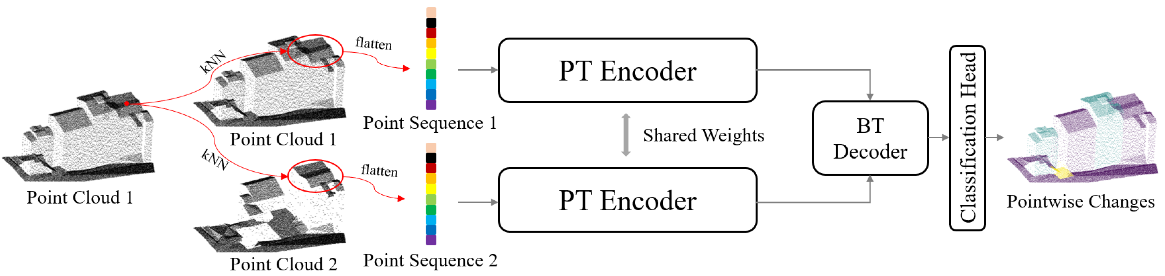
3. Methodology
In this section, we first briefly introduce the process of extracting point sequences. Then, we present how the PT encoder extracts geometric features from point sequences. Finally, we show how the BT decoder learns differential features. The architecture of the proposed PBFormer is shown in
Figure 1.
3.1. Generating Point Sequences
To solve the problem of lacking semantic information at a single point, we calculate the change category of each 3D point from two sequences generated by searching neighbor points in two periods, respectively, with kNN [
52,
53]. The idea of kNN is intuitive, simple, and efficient, retrieving the k-nearest points as a neighborhood by Euclidean distances.
Suppose we have two sets of point clouds
S1n1×c and
S2n2×c, where c is the number of channels and n
1 and n
2 are the number of points in
S1 and
S2, respectively. First, we build kd-trees [
54] for
S1 and
S2 to accelerate the retrieval computation. Then, according to the
k value of kNN, we use kd-trees to retrieve two neighborhoods of a point
pS1 in
S1 and
S2, respectively. The two neighborhoods form a point sequence pair,
P1k×c (
P1S1) and
P2k×c (
P2S2). If there are almost no matching points in S
2 in the same spatial space, kNN is still being executed to generate the second point sequence. Although the neighborhood represented by the second point sequence may be inconsistent with the first one, this difference matches the actual situation (except for occlusion) and provides a pair of point sequences with differences. Finally, this pair of point sequences is fed into PBFormer for CD. The procedure is the same for detecting points in
S2.
Since the bitemporal point clouds do not have strict correspondence, the consistency of the two sequences may also be affected. However, when the appropriate k value is set, the region represented by the two sequences may be approximately the same, and the geometric structure information contained in them will also be approximately the same. If similar regions cannot be obtained, there are likely obvious structural changes.
3.2. Point Transformer Encoder
In order to capture the relationship between points in a sequence, it is necessary to adopt an appropriate method for adding positional embeddings. There are three common choices: none, fixed, and learned [
55]. Without additional positional information, embeddings of the input sequence are immediately fed into the encoder. The fixed method generates a series of positional encodings using a specific function, such as sine and cosine functions. The learned method usually uses learned positional embeddings to encode spatial information, and the dimension of the learned positional embeddings can vary according to the data structure.
Transferring transformers to point cloud learning, we first consider a point sequence P k×c as a sequence with relative position information, where k is the number of points in P and c is the number of the feature dimensions of a point p c in P. In the raw point clouds, the format of p is usually the coordinate (x, y, z) concatenated with the intensity Int. and the true RGB color (r, g, b). Note that the positional information is contained in the original feature of p. Suppose we further consider P as a sequence distributed in 3D space; (x, y, z) can serve as positional encoding. It is also noteworthy that (x, y, z) represents the absolute positional information of p in the entire point cloud. If we only consider the geometric structure at the local spatial scale, the absolute positional encoding changes with the rigid transformation, and it is thus not very robust to jitter, while the relative positional encoding merely reflects the distance xdist between p and a reference point pr, which is invariant to the rigid transformation.
In GCN [
10], the combinatorial Laplacian matrix
L is introduced to replace the adjacency matrix
A, i.e.,
L =
D −
A, where
D is the degree matrix. The Laplacian matrix
L can help GCN reduce the complexity and simplify the process of computing convolution because convolution is easier to calculate in the Fourier domain, and the process of the spectral decomposition of the Laplacian matrix is relatively simple. A recent work [
37] also defines an operator analogous to the discrete Laplacian matrix that uses the identity matrix
I to approximate the degree matrix and the product of the query matrix
Q and the key matrix
K in self-attention networks to the adjacency matrix. This operator can also effectively improve the performance of the model in [
37]. In fact, we find that a feature representing offset also plays an important role in other point cloud learning algorithms [
20,
38], regardless of whether we derive this offset feature in low-dimensional or high-dimensional feature space. Since arbitrary points in
P can be moved to
pr by a certain corresponding transformation matrix
T,
xdist can be expressed as:
where
T is comparable to the adjacency matrix
A. Similarly, we could obtain an approximate discrete Laplacian
Ldist, which provides a way to add positional encoding. Therefore, we simply revise an original coordinate as a positional embedding, called self-positional embedding (SPE), as follows:
where
is a simple mapping function such as FCN to approximate
Ldist, and
pr is the point used to generate
P. We also add LN to improve stability and convergence during training.
The efficient implementation of the original transformer is almost out of the box in ViT. We also purposely followed the mainstream transformer architecture to introduce as little inductive bias as possible.
Our proposed network is illustrated in
Figure 2. To handle 3D point clouds, we consider the neighborhood
P = {
p1,
p2, …,
pk} of each point
p comparable to a flattened 2D patch in ViT and map
P into a linear projection to make point embedding
E k×d, where
d is the number of channels after mapping. We have
where
represents simple mapping functions, such as FCN.
Then, we extract the coordinates of all points in
P, map them into SPE
Es−pos k×d, and add
Es−pos to
E. Thereafter, an extra learnable embedding
XCLS−0 d similar to BERT’s special [
CLS] token, is prepended to the beginning of the
E. During training,
XCLS−0 could learn the category of
pr from the geometric structure of
P. We have
and
where
represents simple mapping functions such as FCN.
Eventually,
X is fed into the transformer encoder, which outputs a [
CLS] token
XCLS d and point features
XPF (k−1)×d. The transformer encoder is composed of
l basic blocks. Each block has two elementary layers, MSA and MLP, followed by LN and residual connections. The operation in the
lth block can be expressed as:
and
Let X = {x1, x2, x3, …, xk}, so XCLS = {x1} and XPF = {x2, x3, …, xk}. Therefore, the outputs of two branches in PBFormer can be expressed as Xb = {XCLS-b, XPF-b} and Xa = {XCLS-a, XPF-a}, where b and a mean before and after.
3.3. Bi-Spatiotemporal Crossing Transformer Decoder
After acquiring two features in different periods, the difference in space between them needs to be further analyzed. The change result
y can be expressed as:
where
f is a function for learning the difference.
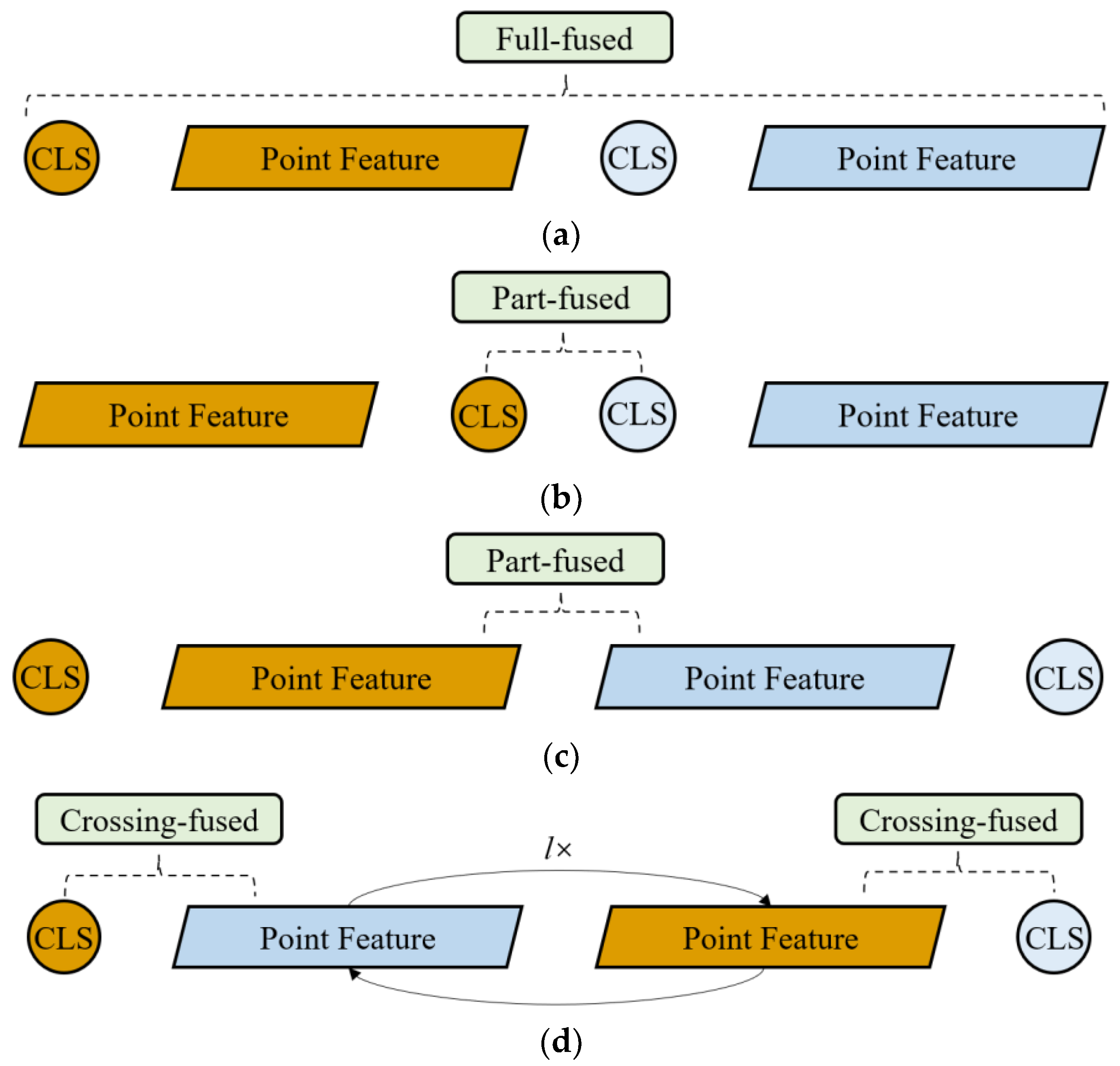
Nevertheless, f implemented by simple network architectures may be laborious for learning complex changes because they only perform comparison operations, and scarcely establish contextual relationships between different temporal features. Therefore, we attempt to take an appropriate approach of fusing Xb and Xa, and propose a well-designed feature fusion network based on the powerful sequence encoding ability of transformers.
There are mainly three types of fusion algorithms: full-fused, part-fused and crossing-fused [
32]. Full-fused means that all features in
Xb and
Xa participate in each operation of
f, as shown in
Figure 3a. However, it is unacceptable because such fusion requires considerable computing time.
Figure 3b,c shows two types of part-fused processing, one with only the point features fused, and the other with only the [
CLS] token fused. Obviously, the key information of the two representations is not fully exploited.
According to the correspondence of the scene before and after changes, the change in the representation in one period could be captured by the other representation. Thus, we try to achieve this goal by exchanging information in two representations, as shown in
Figure 3d. This scheme, called crossing-fused, considers two point features as mediums for exchanging information. Throughout the fusion process, the two mediums successively transmit their information to two [
CLS] tokens.
First, XPF-b carries the spatial structure information before changes, and XCLS-a indicates that the changes are fused; then XCLS-a is fused with XPF-a again. In this process, XCLS-a learns useful spatial features before and after the change. Second, XCLS-b is subjected to the same computation as XCLS-a, where XPF-b and XPF-a replace each other. Third, the above process is repeated l times to obtain two adequately fused [CLS] tokens.
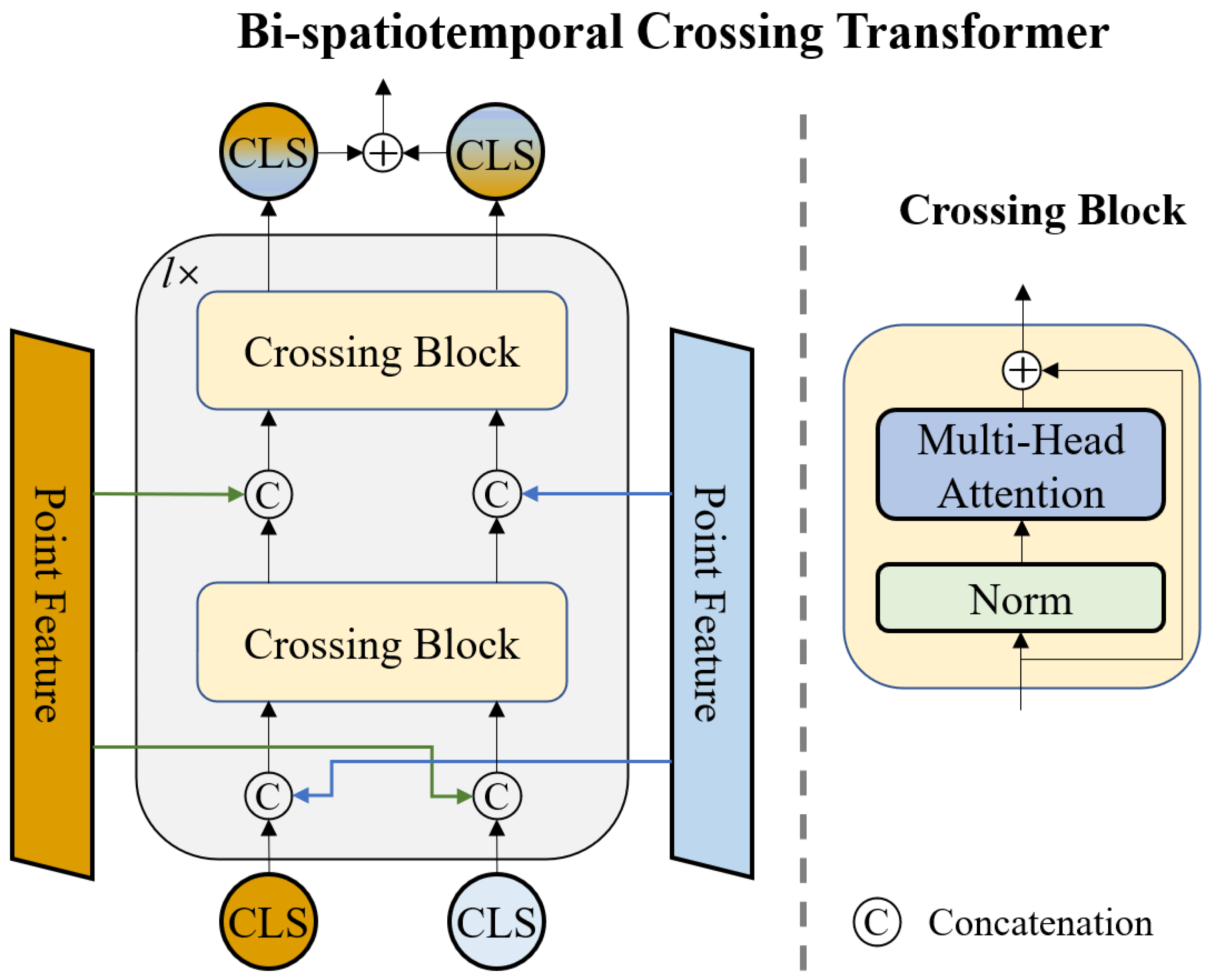
The proposed feature fusion module based on a crossing-fused scheme is shown in
Figure 4. Since transformers have the ability to capture long-range interactions and dependencies, we implement each fusion operation using a simple transformer network called the crossing block. Our crossing block consists of MSA, followed by LN and residual connections. After
l times of crossing fusion, we obtain two fused [
CLS] tokens. During this process of crossing fusion, the two [
CLS] tokens could learn geometric structure information at the other branch. The operational process of a branch in the BT decoder can be expressed as:
where
i = 1, 2, 3, …,
l. Finally, the
l-th
XCLS-bd is added to the
l-th
XCLS-a d and fed into a classification head implemented by MLPs.
4. Experiments
In this section, we evaluate PBFormer through extensive experiments. First, the experimental setup is presented in detail. Second, PBFormer is compared to several methods that present results at different levels. Third, the relationship between training set size and model performance is analyzed. Finally, ablation studies are performed for our SPE and BT decoder.
4.1. Setup
The Urb3DCD [
34] is an urban point cloud dataset based on the 3D model of a real city with level of detail 2 (LoD2) precision. Urb3DCD consists of 5 sub-datasets, which are divided according to the resolution and noise level. The sub-dataset-1 provides 3 different training sets: 1-a is a small training set, with only 1 pair of point clouds; 1-b is a normal training set, with 10 pairs of point clouds like the others in sub-datasets-2, 3, 4 and 5; 1-c is the largest training set, with 50 pairs of point clouds. There is 1 pair of point clouds in the validation set and 3 pairs of point clouds in the test set for all sub-datasets. The raw 3D points in Urb3DCD contain only 3D coordinates, without color and intensity information, and can be divided into 3 classes: new, demolished, and unchanged.
Our proposed PBFormer was implemented with PyTorch. All experiments were conducted on the same machine with an Intel i9-10900K @3.7GHz CPU and an NVIDIA RTX3060 GPU. The AdamW optimizer was used, without changing any parameters. The initial learning rate was set to 0.0002 and scheduled by cosine annealing, with warm restarts at each step. For the evaluation on Urb3DCD and analyzing the influence of the training set size, the model was trained for 50 epochs. The batch size was set to 32, and the number for cutting point sequences, k, was set to 256. Cross-entropy was adopted as the loss function. We stacked 4 transformer encoders in the PT encoder and 4 crossing blocks in the BT decoder. During training and testing, the whole raw point clouds are fed into PBFormer to detect pointwise changes without projecting, rasterizing, and tiling.
The mean intersection over union (mIoU) can be used to measure the similarity between predicted results and the ground truth and evaluate an algorithm’s performance. Therefore, our experiments use the mIoU of all change categories as the standard metric. Let
Mconfusion be the n × n confusion matrix; then, mIoU can be expressed as:
where true positive (TP) indicates the number of points that change in ground truth and as well as in the predicted point clouds, false negative (FN) represents the number of points that change in ground truth but do not change in the predicted point clouds, and false positive (FP) is the number of points that do not change in ground truth but do change in the predicted point clouds.
4.2. Change Detection on Benchmark
Five well-established methods are selected for comparison and verification of the effect of the proposed PBFormer. (1) Methods based on DSM difference (DSMd) [
56] with empirical thresholds are applied to process 2D images generated from DSMs and are displayed at the 2D pixel and patch level. (2) A Siamese FFN [
48] and a Siamese convolutional neural network (CNN) [
47] are applied to detect 2D images, but they are only displayed at the 2D patch level. (3) The cloud-to-cloud (C2C) [
57] is a comparison method at the 3D points level which is based on point-to-point Hausdorff distance. C2C cannot discriminate the change category, providing only binary results. (4) The multi-scale model-to-model cloud comparison (M3C2) [
58] method uses a hand-crafted feature based on the distance along the normal direction between two point clouds, and M3C2 also provides results at the 3D point level. (5) A random forest (RF) algorithm with the hand-crafted stability feature (SF) [
14] can provide results at the 3D point level.
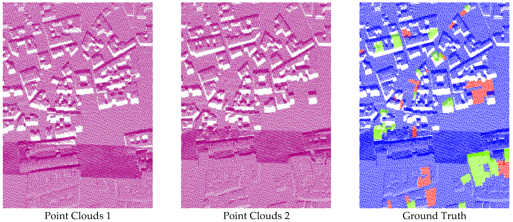
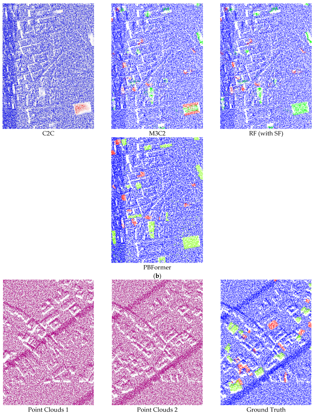
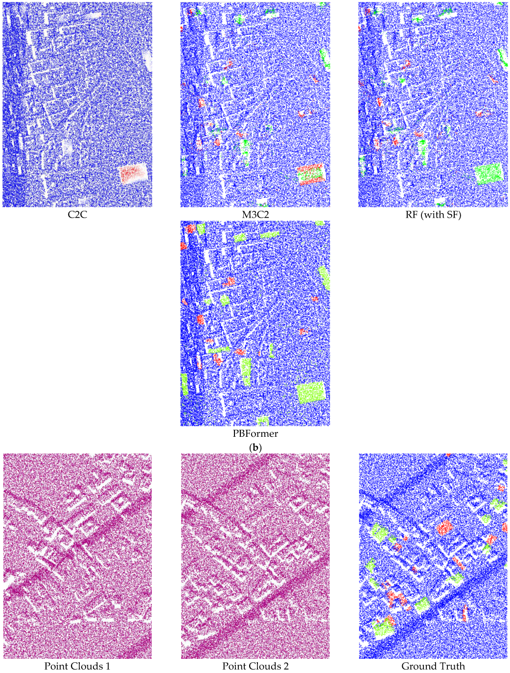
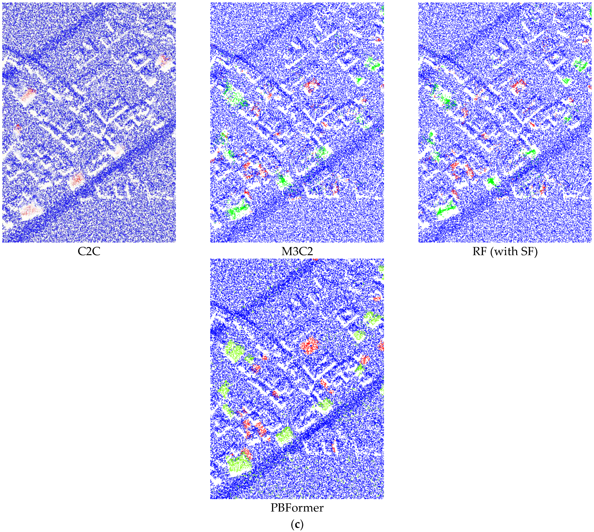
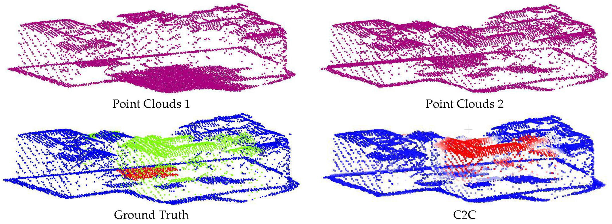
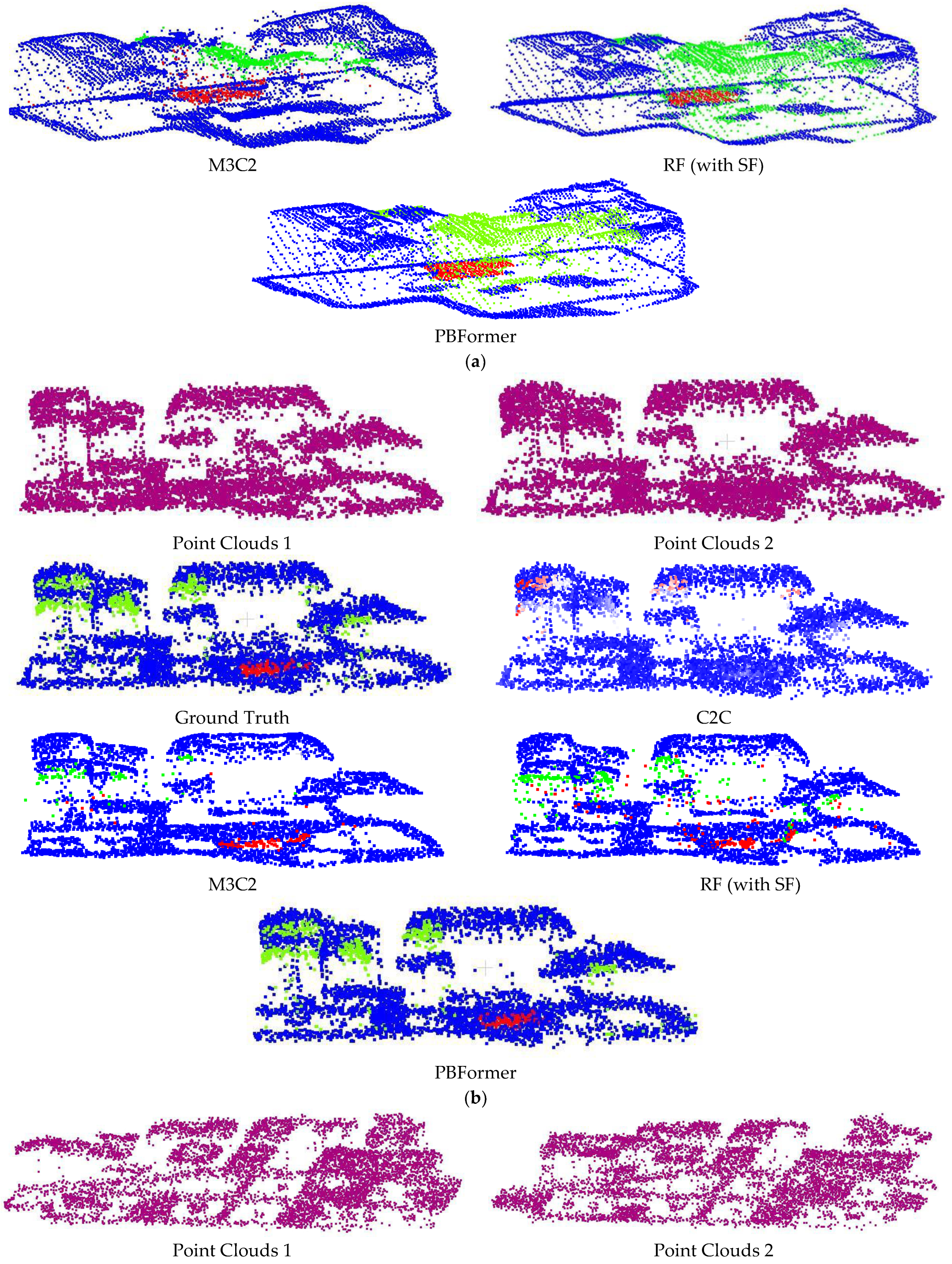
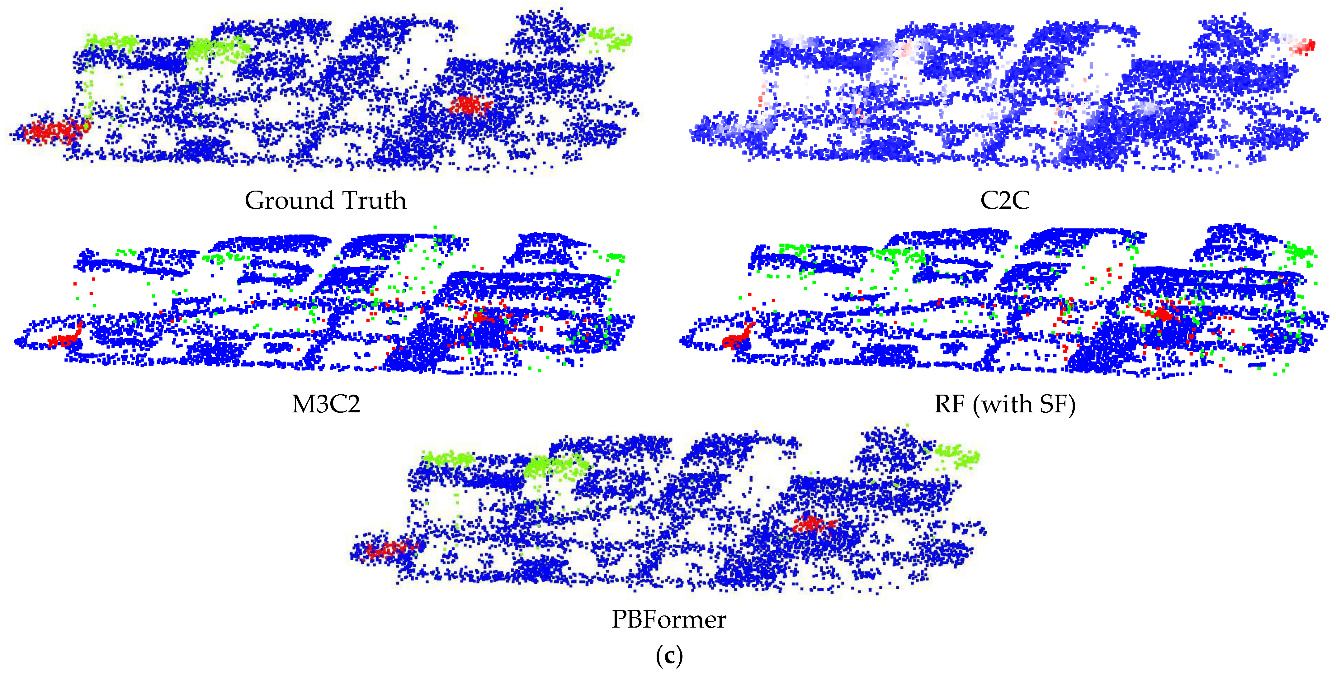
The effectiveness of PBFormer is evaluated on all standard-sized sub-datasets by comparing our method with other excellent methods, both qualitatively and visually. The quantitative comparison is shown in
Table 1, and the qualitative results are visually presented in
Figure 5 and
Figure 6.
It can be seen that: (1) The results of methods processing DSMd with empirical thresholds consistently failed to perform satisfactorily on all sub-datasets. Otsu’s threshold algorithm [
59] and the opening filter [
60] can significantly improve the performance, meaning that nearly all of their results achieved more than 80% of mIoU. However, in these results, we can observe the change of 3D point clouds only from the top view. (2) FFN and Siamese CNN showed inconspicuous results despite being trained. A possible reason is that the two networks have simple architectures and are not specially designed for point clouds. (3) C2C only provided binary results, and the accuracy was directly determined by the empirical threshold. Although we additionally used the fuzzy threshold, it is still unsatisfactory, even in terms of visual effect (as shown in
Figure 5a–c). (4) M3C2 achieved results close to the lowest mIoU. This hand-crafted feature is not robust enough, especially when there is excessive noise in the point clouds. (5) The RF (with SF) algorithm also obtained merely ordinary results due to the limitation of hand-crafted SF. (6) Last but not least, our PBFormer outperforms the above approaches regarding mIoU and performs better on 5 sub-datasets.
We further explored the relationship between the size of the training set and the performance of the model, as shown in
Table 2. It can be seen that: (1) When training models on sub-dataset-1-a (including only 1 pair of point clouds), the mIoU score of our PBFormer is lower than those of the FFN and RF (with SF). The reason for this is that transformers have more powerful modeling flexibility and less inductive bias, so they generally needs to be supported by large-scale datasets. Therefore, it is challenging to train PBFormer on a small-scale training set, which leads to slightly poor results in our approach. (2) Increasing the training set size is an effective solution to improve the detection accuracy, which is more obvious in FFN and our PBFormer. Although the result obtained on sub-dataset-1-b (10 pairs of point clouds) was used as a baseline in our work, our PBFormer may achieve better performance when supported by more data, such as training on sub-dataset-1-c (50 pairs of point clouds).
4.3. Ablation Studies
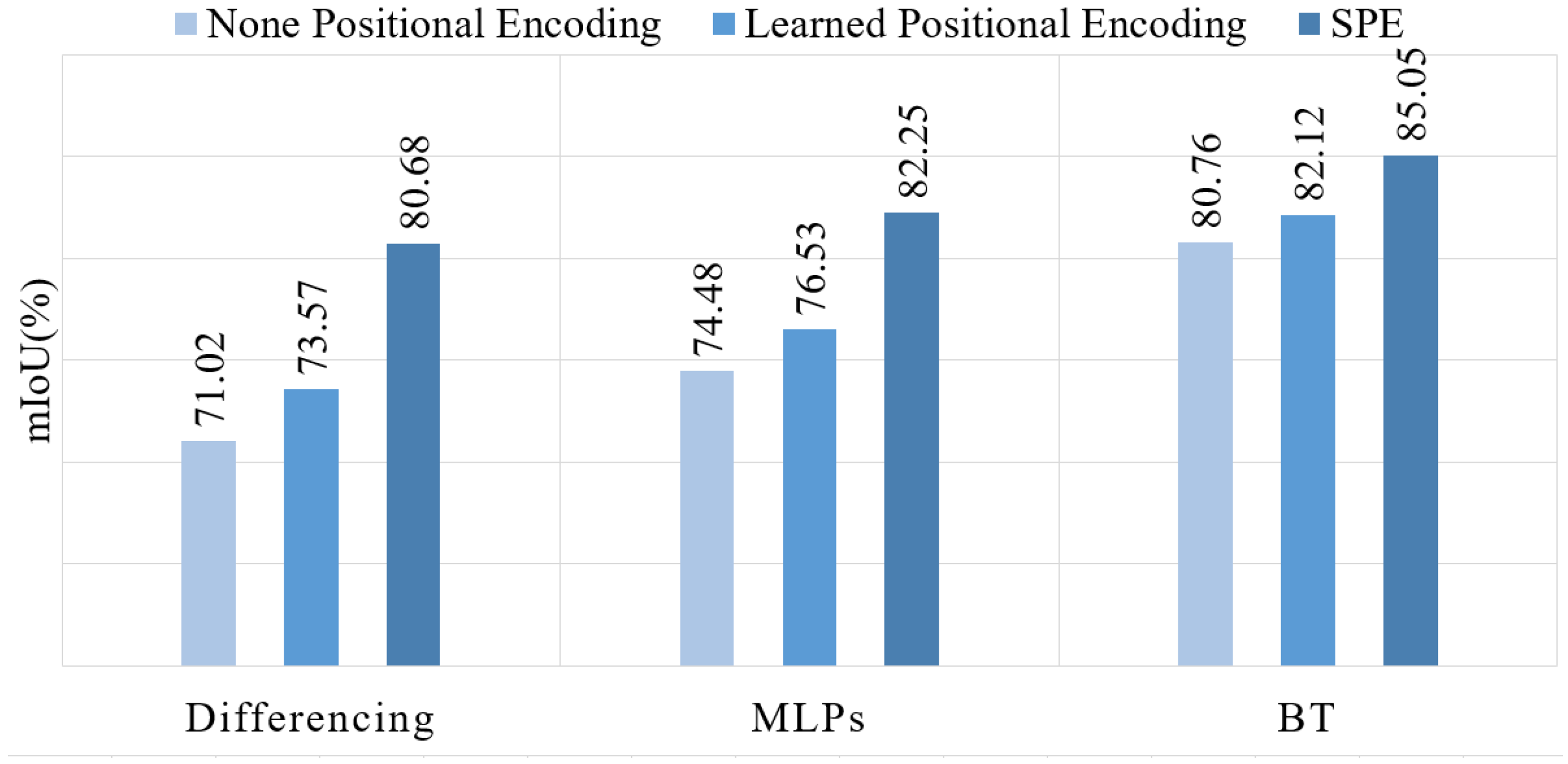
In this section, we first compared the different positional encoding strategies to illustrate the necessity of our proposed SPE. Then, we analyzed the BT decoder’s effectiveness by training ablated networks with other feature fusion modules. All ablated networks were trained on the sub-dataset-1-b and evaluated on the test set in sub-dataset-1.
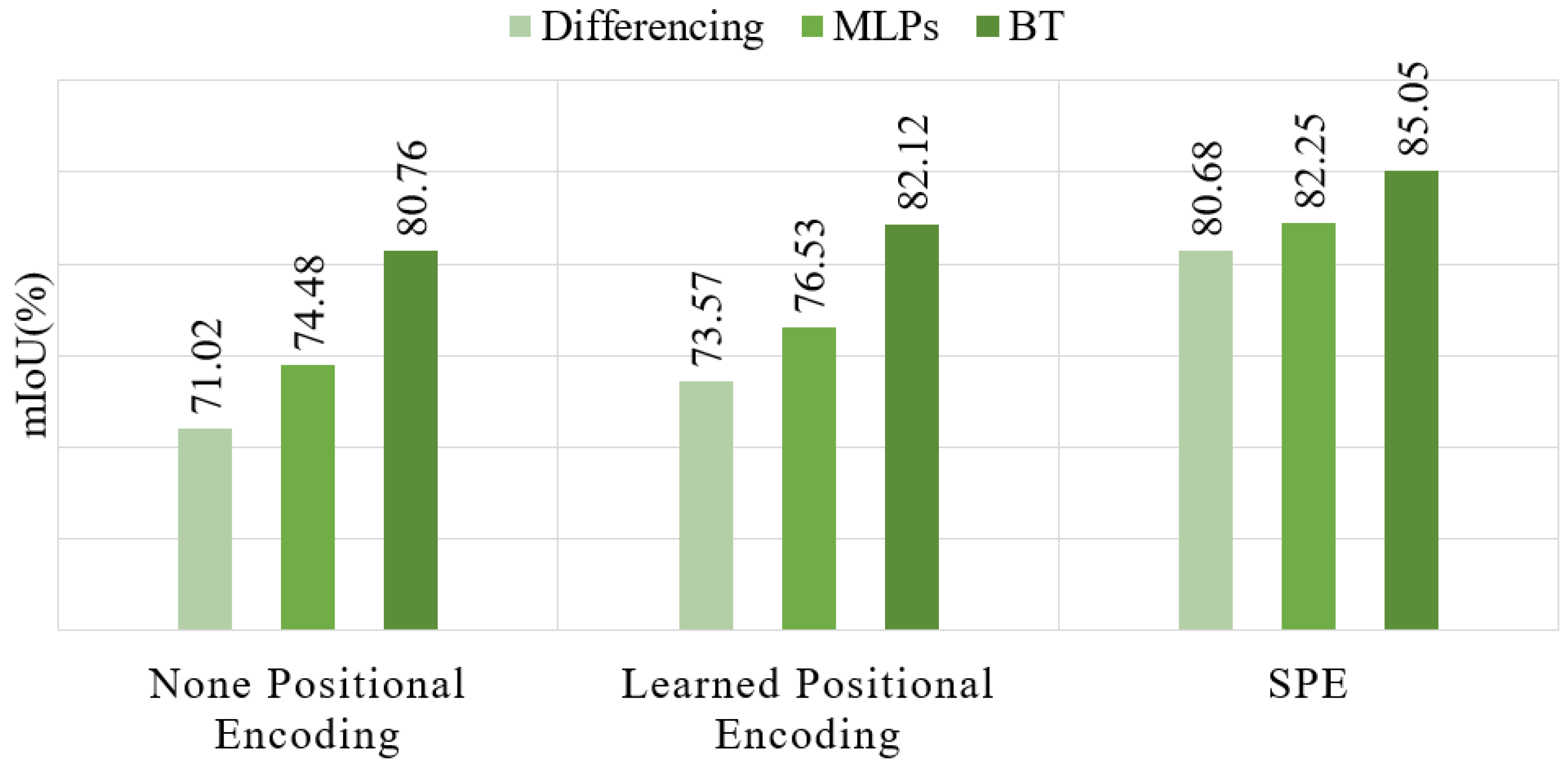
Expecting to evaluate the full network (PBFormer), we conducted eight ablation experiments: (1) Removing SPE and replacing BT by differencing. After removing SPE and BT, we used a pair of sharing transformer encoders of ViT, without position embedding, as Siamese encoders and differencing as the method of feature fusion. (2) Replacing SPE with learned positional encoding. Compared to (1), we added widely used learned 1D positional embeddings to the point embedding sequence in the transformer encoder of ViT. (3) Applying SPE and differencing. In this ablation experiment, SPE was added to the ablated network in (1). (4) Removing SPE and replacing differencing by MLPs. In this ablation experiment, differencing was replaced, and MLPs were considered as the feature fusion module. (5) Applying learned positional encoding and MLPs. We added learned 1D positional embeddings to the ablated network in (4). (6) Applying SPE and MLPs. SPE was added to the ablated network in (4). (7) Removing SPE and applying BT decoder only. In this ablation experiment, MLPs were replaced by our BT decoder. (8) Applying learned 1D positional embeddings and the BT decoder. In the last ablation experiment, learned 1D positional encoding was added to the ablated network in (7).
Table 3 shows the mIoU scores in all ablation experiments.
Figure 7 shows the comparative results obtained by varying the positional encoding strategy, and
Figure 8 shows how varying feature fusion modules affect the results.
It can be seen that transformer networks have a strong feature extraction ability, which is the prerequisite for the design of PBFormer. Even using only the basic transformer encoder, the mIoU score can easily exceed 70. Moreover, positional embeddings facilitate transformer networks learning point sequence, and a widely used method of positional encoding can improve the mIoU score. In addition, our proposed PT encoder with SPE has one of the most significant impacts on performance. Regardless of the type of feature fusion module used, mIoU scores above 80 demonstrate that SPE is necessary for transformer networks to effectively learn spatial structure information from 3D point clouds.
Moreover, the replacement of the feature fusion modules shows that the BT decoder has another significant impact on performance. The mIoU score also exceeds 80 when only the BT decoder is used in PBFormer. Similarly, based on three positional encoding strategies, the mIoU scores over 80 prove that the BT decoder could effectively learn the difference between bitemporal point clouds.
Finally, the complete model was evaluated, and it achieved superior performance. The role of the SPE and BT decoder and how they cooperate with each other to achieve the best results was demonstrated in the above ablation experiments.
5. Discussion
This section provides a discussion to explain the previous experimental results. The discussion includes further elaboration of the experimental results and the influence analysis of the experimental dataset.
In this paper, PBFormer was compared with other methods regarding the Urb3DCD benchmark. In addition to the better results achieved with our network, several issues remain to be addressed. With sufficient prior information, C2C is still a method worth considering due to its high efficiency. However, due to its over-dependence on the threshold and its ignoring of the local geometric structure, C2C usually fails to achieve satisfactory results. For a better visual effect, we tried to blur the threshold and obtained some faded areas in
Figure 5 and
Figure 6, but the result was not perfect. Although the centers of the changed regions can be distinguished, the boundaries between the changed and unchanged regions are vaguer. The result of M3C2 is also unsatisfactory, both visually and qualitatively. The visual results of M3C2 seem to be smoothed because all corresponding points of the points distributed on the edge are not found by M3C2, and they remain in the gray area. RF (with SF) is more reliable than C2C and M3C2, which are relatively sensitive. While all three belong to the one-stage strategy, the quantitative and visual result of RF (with SF) reflects the gap between machine learning-based and traditional methods. A possible reason for the poor results of M3C2 and RF (with SF) is the lower resolution of the dataset. Even for the sub-dataset-2, the resolution is about 10 points/m
2. In this case, where the detection (LODetection) level may exceed the magnitude change, M3C2 applied to detect changes at the centimetric scale will perform less well on a dataset at the metric scale. This could explain the less adequate result of RF (with SF) on sub-dataset-1 (0.5 point/m
2) and the improvement in sub-dataset-2. PBFormer is also affected by the resolution, and point clouds with a higher resolution help PBFormer to achieve better CD quality. However, when processing sparse point clouds, PBFormer could still obtain enough points to learn the characteristics between two inputs by kNN, which is part of the reason why PBFormer works better than other methods.
The establishment of the Urb3DCD benchmark is a pioneering work that provides a dataset with pointwise annotations for training deep learning-based models. However, the scenario in Urb3DCD is simplified, where only ground data appear (with the exception of buildings), and there are few occluded building point clouds. Due to the gap between the dataset and the real world, the generalization ability of PBFormer might be lower than expected. In addition, the categories of changes only include ‘new buildings’ and ‘demolished buildings’, which may cause PBFormer to merely learn whether there has been a change, but not the semantics of the point clouds. Moreover, a problem that cannot be ignored and avoided is the data imbalance. In the data used for CD, there are usually fewer changed areas with respect to unchanged areas, which is unfavorable for PBFormer, which is designed based on the assumption that the distribution of each class of samples is uniform. Finally, it should be noted that PBFormer may have poor performance at the boundaries between changed and unchanged objects, especially when the noise is high. PBFormer is a network that outputs pointwise changes. If the edges of buildings are blurred by the high noise, PBFormer would not adequately understand the structure of buildings.


