Accuracy Assessment of High-Resolution Globally Available Open-Source DEMs Using ICESat/GLAS over Mountainous Areas, A Case Study in Yunnan Province, China

Abstract

The Open-Source Digital Elevation Model (DEM) is fundamental data of the geoscientific community. However, the variation of its accuracy with land cover type and topography has not been thoroughly studied. This study evaluates the accuracy of five globally covered and open-accessed DEM products (TanDEM-X90 m, SRTEM, NASADEM, ASTER GDEM, and AW3D30) in the mountain area using ICESat/GLAS data as the GCPs. The robust evaluation indicators were utilized to compare the five DEMs’ accuracy and explore the relationship between these errors and slope, aspect, landcover types, and vegetation coverage, thereby revealing the consistency differences in DEM quality under different geographical feature conditions. The Taguchi method is introduced to quantify the impact of these surface characteristics on DEM errors. The results show that the slope is the main factor affecting the accuracy of DEM products, accounting for about 90%, 81%, 85%, 83%, and 65% for TanDEM-X90, SRTM, NASADEM, ASTER GDEM, and AW3D30, respectively. TanDEM-X90 has the highest accuracy in very flat areas (slope < 2°), NASADEM and SRTM have the greatest accuracy in flat areas (2 ≤ slope < 5°), while AW3D30 accuracy is the best in other cases and shows the best consistency on slopes. This study makes a new attempt to quantify the factors affecting the accuracy of DEM, and the results can guide the selection of open-source DEMs in related geoscience research.

1. Introduction

The digital elevation model (DEM) is fundamental data of the geoscientific community. The DEM and its derived properties (slope, aspect, curvature) are essential parameters for terrain evaluation [1]. DEM error propagates in the whole data processing process, resulting in deviation of the precision of the results. Thus, an accurate DEM is desirable for geoscientific applications.

There are ready-made open-source DEM products with global coverage, such as TanDEM-X DEM [2] with a 90-m resolution, SRTM DEM [3], NASA DEM [4], ASTER GDEM [5], AW3D30 DEM [6] with a 30-m resolution. The nominal accuracies of the DEM products have been officially reported based on an overall error on a global scale or within the coverage of DEM [7]. However, the DEM error will deviate from the official value in the local area [8]. Various datasets use different techniques to generate DEM, which will cause the consistency of DEM quality to be different under different terrain conditions and land cover types [9].Therefore, it is crucial to evaluate the quality of DEMs quantitatively. More importantly, the influence of regional topographic conditions or land cover on the accuracy of DEM products needs to be investigated.

There are mainly two methods for evaluating different DEM datasets [10]. One approach is to compare a DEM to a higher-accuracy DEM, such as high-quality DSMs generated by small-scale airborne LiDAR or stereo imaging [8,11]. Another approach is to compare the DEM with ground control points (GCPs), such as elevation control points, GNSS data, and the Ice, Cloud, and Land Elevation Satellite/Geoscience Laser Altimeter (ICESat/GLAS) data collected from large-scale topographic maps [12]. Thus, the ICESat/GLAS elevation data product with global coverage is the reasonable alternative where absolute reference data are limited [13].

This study aims to evaluate the quality of five open-source DEMs (TanDEM-X90 m, SRTM V1, NASA DEM, ASTER GDEM, and AW3D30) in areas with substantial terrain relief, complex terrain geological, and variable vegetation coverage. The quality of a digital elevation model (DEM) is not only determined by its vertical accuracy, but also by the consistency of its accuracy under different geographic conditions. Our study includes the following works: (1) We demonstrate the non-normal distribution of DEM errors and choose more robust metrics accordingly. (2) Our study provides insights into the effects of slope, orientation, land cover type, and vegetation cover on DEM accuracy under complex geographic conditions, and explores the consistency of DEM quality under these conditions. (3) We introduce the Taguchi method for the first time to quantify the effects of these factors on DEM accuracy by calculating the factor contribution. This will provide an important reference for improving the quality of DEM in mountainous areas and help users select the most suitable open-source DEM for different geographic conditions.

This paper is structured as follows. Section 2 presents the study area and the datasets used in this study. The methodology is given in Section 3, including preprocessing of DEM products and the ICESat GCPs, quality assessment of DEMs, and the impact factor analysis with the Taguchi model. Section 4 presents the quality assessment and analysis results. Section 5 discusses the reasons for the differences in the accuracy of various DEMs, and some concluding remarks are provided in Section 6.

2. Study Area and Datasets

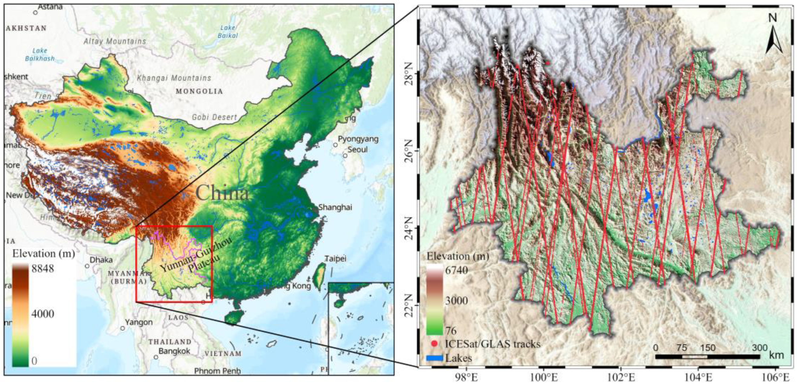
2.1. Study Area

Yunnan Province, located in southwestern China, as shown in Figure 1, has substantial terrain relief and various geomorphic coverage, making it an ideal area to evaluate different DEM products. The topography is dominated by mountains and intervening valleys. Unique geographical conditions at high elevations and low latitudes have formed various types of landforms, such as hills, lakes, grasslands, snow mountains and forests, as well as highly diverse vegetation types and covers. Hence, this region has a good representation for evaluating the accuracy of different DEMs.

2.2. DEMs

This study compared five commonly used open-source DEM datasets with global coverage. The basic parameters of these DEMs are listed in

Table 1. Basic parameters of DEM datasets used in this study.

DEM	Primary Source	Resolution	Producer	Datum Plain/Vertical	Vertical Accuracy	Acquired
TanDEM-XDEM	X band SAR	3″ (~90 m)	DLR	WGS84/WGS84	<10 m (LE90) [16]	2011–2015
SRTM (v3)	C band SAR	1″ (~30 m)	NASA	WGS84/EGM96	<16 m (LE90) https://www2.jpl.nasa.gov/srtm/ (accessed on 1 April 2023)	1999–2000
NASA DEM	Reprocessed C band SAR	1″ (~30 m)	NASA	WGS84/EGM96	Not reported	1999–2000
ASTER GDEM (v3)	Stereo NIR imagery	1″ (~30 m)	NASA/METI	WGS84/EGM96	~8.5 m (RMSE) [17]	2000–2008
ALOS World 3D AW3D30	Stereo pan imagery	1″ (~30 m)	JAXA	WGS84/EGM96	~4.4 m (RMSE) [18]	2006–2011

. It is worth noting that the five global elevation models used in this paper are all digital surface models (DSM) [7,14]. However, for most applications, they are considered equivalent to digital elevation models (DEMs) [15]. Therefore, for the sake of simplicity, we will use the term “DEM” in the rest of the paper.

2.2.1. TanDEM-X 90 m DEM

The TanDEM-X DEM was produced by the TanDEM-X mission operated by the German Aerospace Centre (DLR) and Airbus. Two identical X-band synthetic aperture radar satellites fly in close formation in orbit at an altitude of approximately 500 km. Several scenes were collected from December 2010 to January 2015 for DEM production, with all landmasses being imaged at least twice and up to seven or eight times [16]. A global digital elevation model, TanDEM-X DEM, with a resolution of 0.4 arcsec (approximately 12 m at the equator), was generated in September 2016 [2]. The absolute vertical accuracy is less than 10 m (LE90), and the relative vertical accuracy is less than 2 m in the areas with a slope less than 20% and 4 m when the slope is larger than 20% [16]. The TanDEM-X 90 m DEM is derived from the TanDEM-X DEM by reducing the pixel spacing from 0.4 arcsecs to 3 arcsecs (approximately 90 m at the equator). It is freely available worldwide and used in this study.

2.2.2. SRTM

The Shuttle Radar Topography Mission (SRTM, https://earthexplorer.usgs.gov/, accessed on 1 April 2023) was completed with the cooperation of NASA, the National Geospatial-Intelligence Agency (NGA), and the German and Italian space agencies. The SIR-C/X SAR instrument with two antennas onboard the Space Shuttle Endeavour captured the global surface from 60°N to 56°S during an 11-day flight in February 2000. C-band radar generated a continuous mapping, while X-band radar only acquired data from discrete swaths 50 km wide. A DSM covering 80% of the global landmass was generated by single-pass cross-track SAR interferometry [3]. The latest official version SRTM_v3 mainly used the ASTER GDEM to fill the voids existing in the previous versions of SRTM (NASA 2015). The accuracy of the SRTM with a 1 arcsec (~30 m) grid size is specified as better than 16 m (absolute) and better than a 10 m (relative) vertical elevation error. The 1 arcsec SRTM used in this study was globally released in September 2014.

2.2.3. NASA DEM

The NASA DEM [4], released by NASA on 18 February 2020, is the successor of SRTM_v3 and is produced by reprocessing the whole SRTM raw radar signal with elevation correction and void filling. The ICESat/GLAS data were used as the ground points to improve the vertical accuracy, swath consistency, and uniformity within the swath mosaic. ASTER GDEM v3, AW3D30 DEM, USGS National Elevation Dataset (NED), and Canadian and Alaskan DEMs were used to fill in the voids during processing. The vertical accuracy has yet to be officially released. Its accuracy has been independently evaluated over various regions, with RMSE ranging from 3.1 m to 6.59 m [19]. The NASA DEM has slightly improved in vertical accuracy compared to the SRTM DEM [20].

2.2.4. ASTER GDEM

ASTER GDEM (https://asterweb.jpl.nasa.gov/gdem.asp, accessed on 1 April 2023) data are jointly developed by Japan’s Ministry of Economy, Trade, and Industry (METI) and NASA and distributed free to the public. The ASTER GDEM product is produced by stereo images obtained by the Advanced Spaceborne Thermal Emission and Reflection Meter (ASTER) onboard the Terra satellite. The images are acquired in the near-infrared wavelength (0.78–0.86 μm), covering 99% of Earth’s landmass for a range from 83°N to 83°S [21]. The latest upgraded version ASTER GDEM v3 was released on 5 August 2019. 360,000 optical stereo pair data have been added, mainly used to reduce blank elevation areas and abnormal water values. The vertical accuracy is slightly improved compared with the second version, with RMSE ranging from 6.92 to 9.25 m across different cover types in the United States [17].

2.2.5. AW3D30

The ALOSWorld3D 30 m DEM (AW3D30, https://www.eorc.jaxa.jp/ALOS/en/aw3d30/data/index.htm, accessed on 1 April 2023) was developed based on millions of images acquired by the Panchromatic Optical Sensor (PRISM) on the Advanced Land Observation Satellite (ALOS) with sensors at nadir, forward, and backward generating three sets of full-color (0.52–0.77 μm) images along the track [6]. The dataset has been updated several times to improve absolute/relative height accuracy with additional calibration and gap filling [6]. The height accuracy was reported to be about 4.4 m (RMSE) using independent checkpoints distributed in the world [18]. The latest version (AW3D30_v3) was released in January 2021. The 5 m resolution dataset is commercially charged, and the 30 m resolution version (AW3D30) is freely available [20].

2.3. ICESat/GLAS

The ICESat/GLAS data were collected by the Geoscience Laser Altimeter System (GLAS) on the Ice Cloud and Land Elevation Satellite (ICESat) between 12 January 2003 and 11 October 2009. The ICESat/GLAS mission was originally launched to monitor ice sheets. Due to the global coverage, the data is widely applied in monitoring other landcover types. The absolute vertical accuracy in measuring the water-level of lakes can reach the centimeter level under suitable conditions [22].

In addition, the laser altimetry dataset has also been proven to have global high-accuracy elevation control points [23]. The accuracy was validated using airborne LiDAR data from six areas worldwide. The root mean square error of the footprint point elevation is 0.57~0.67 m in the flat areas and less than 3 m in the mountainous areas [23]. ICESat/GLAS dataset is an ideal elevation ground control point for evaluating the accuracy of DEM products worldwide. This study uses the L2 product GLAH14 latest version of global land surface height measurement data (V34) from 2003 to 2009, available through the National Snow & Ice Data Center (NSIDC). The vertical reference of the GLAH14 elevation is TOPEX/Poseidon ellipsoid, so it is crucial to convert the height of GLAH4 to the orthometric height of other datasets. For the processing details, see the description in Section 3.

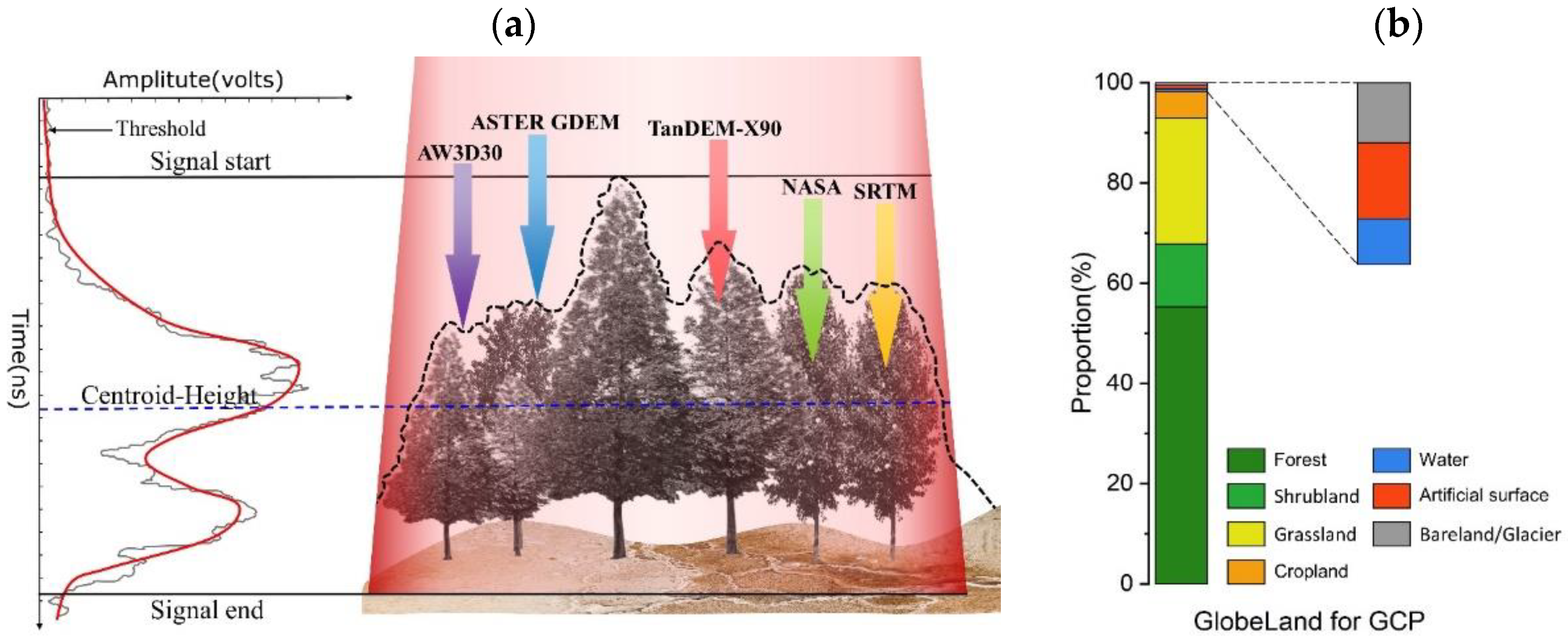
2.4. GlobeLand30 and FVCover Data

GlobeLand 30: National Geomatics Center of China released the 30-m resolution global landcover data product (GlobeLand30) in 2014 and was updated in 2021 [24]. Multispectral images with a resolution of 30 m, including the U.S. Land Resources Satellite (Landsat) TM5, Enhanced Thematic Mapper plus (ETM+), and Chinese Environmental Protection & Disaster Monitoring Constellation (HJ-1), are jointly employed to generate classified images of land cover. The product also uses existing surface coverage data, global MODIS NDVI chronological data, global basic geographic information data, global DEM, and online high-resolution images to support sample selection and auxiliary classification. The overall accuracy was reported to be better than 80%.

FVCover: The Fractional Vegetation Cover (FVCover) corresponds to the ground covered by green vegetation expressed as a percent of the reference area, quantifying vegetation’s spatial extent [25]. FVCover is a good candidate for monitoring the ecosystem since it is independent of light direction and sensitive to the amount of vegetation. Here, we downloaded the data with a 300 m resolution at Copernicus Global Land Services.

3. Methodology

In this study, the accuracy of five open-source DEMs with a consideration of different factors such as slope, aspect, landcover, and vegetation using ICESat/GLAS data as the elevation GCPs. A schematic diagram of the DEM quality evaluation framework is shown in Figure 2. The elevation reference datum of different DEM products and the ICESat/GLAS data need to be unified for comparison. We interpolated the elevation at the ICESat/GLAS ground footprint from five DEMs using bilinear interpolation to examine the elevations with the ICESat-measured values on GCPs. Moreover, we extracted the terrain factors (slope and aspect) and surface coverage factors (GlobeLand30, FVCover) corresponding to GCP for analyzing the relationship between DEM error and these factors.

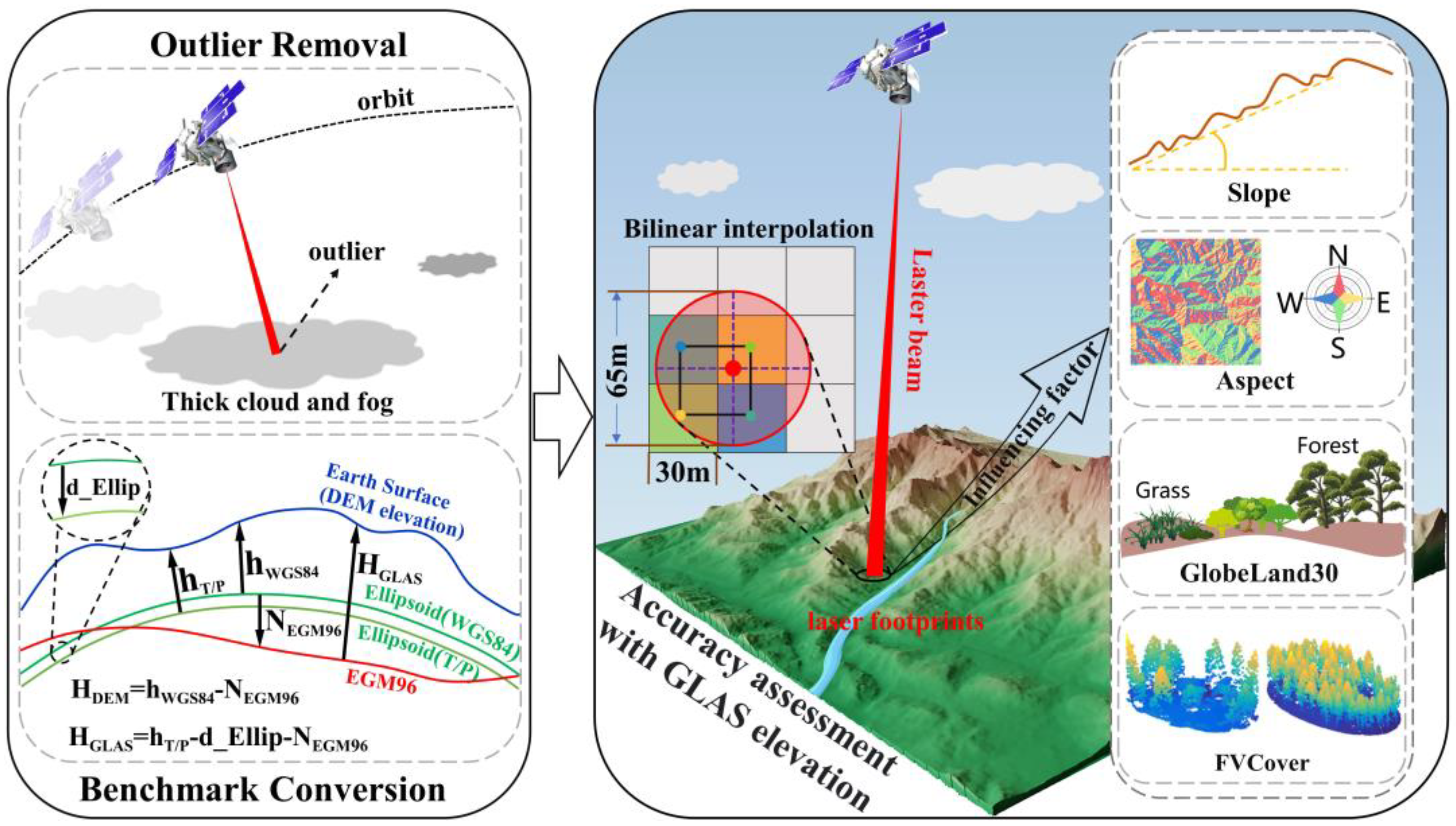
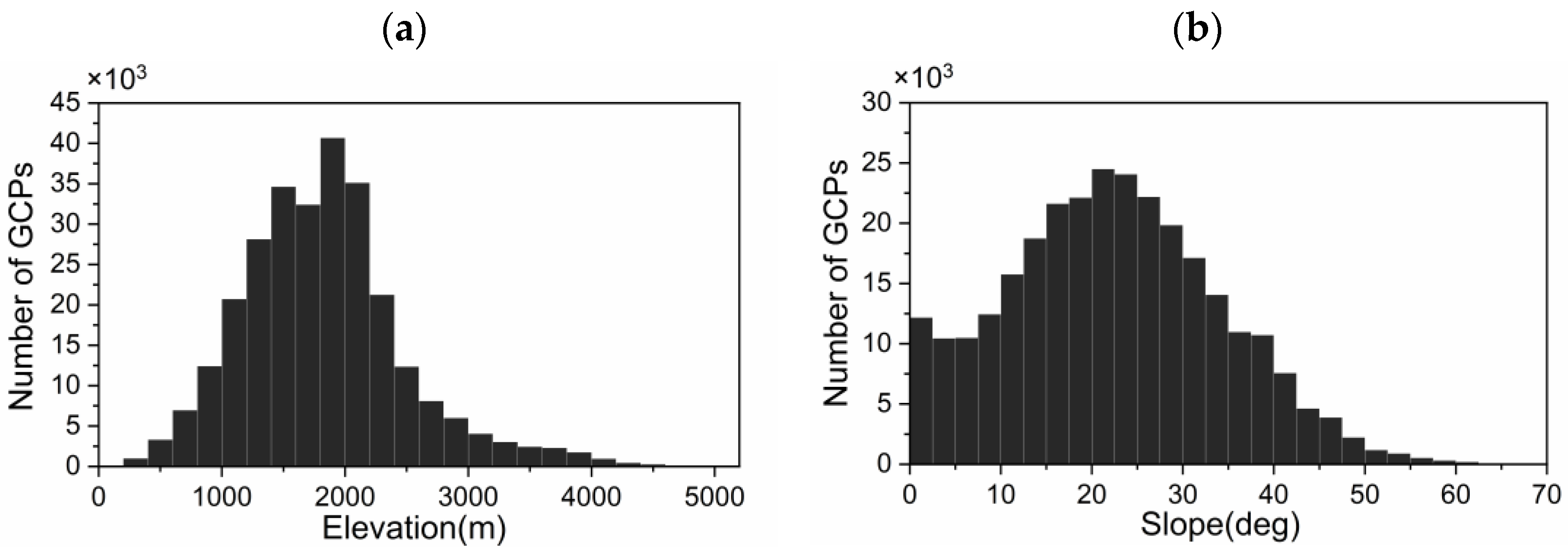
3.1. Preprocessing of GCPs Data and DEMs

Data preprocessing consists of two steps: vertical reference datum conversion and removal of outliers in ICESat/GLAS data. The horizontal reference of all DEM data used in this study is the WGS84 coordinate system, but the vertical references of the five DEM and ICESat/GLAS data are various. The elevation measured by ICESat/GLAS is referenced to the TOPEX/Poseidon ellipsoid, while the TanDEM-X DEM is referenced to the WGS84 ellipsoid. The other four DEM products used in this study are all referenced to the EGM96 geoid. Therefore, we converted the ICESat/GLAS data and the TanDEM-X DEM to the common vertical datum (EGM96 geoid).

According to the quality control results provided by NSIDC, approximately 50% of ICESat/GLAS points are unreliable, which indicates that quality control is necessary [10]. In this study, we select four quality control marks provided by NSIDC, i.e., the elevation usage flag, the cloud flag, the range offset quality flag, and the saturation flag, to eliminate outliers. A total of 586,249 laser footprint points have been obtained in Yunnan Province, and after removing the outliers, there are 277,215 points left. As shown in Figure 3, these points are distributed across various elevations and slopes. However, as indicated in Figure 3b, the number of GCP points with a slope greater than 60° is insufficient to obtain robust statistics. Therefore, the slope statistics in this paper do not include areas with slopes greater than 60°.

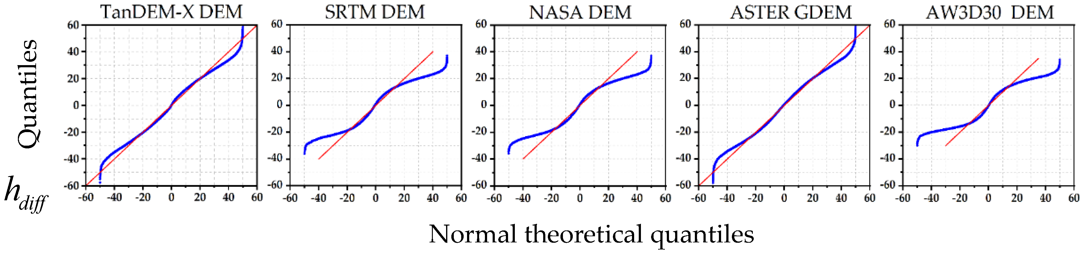
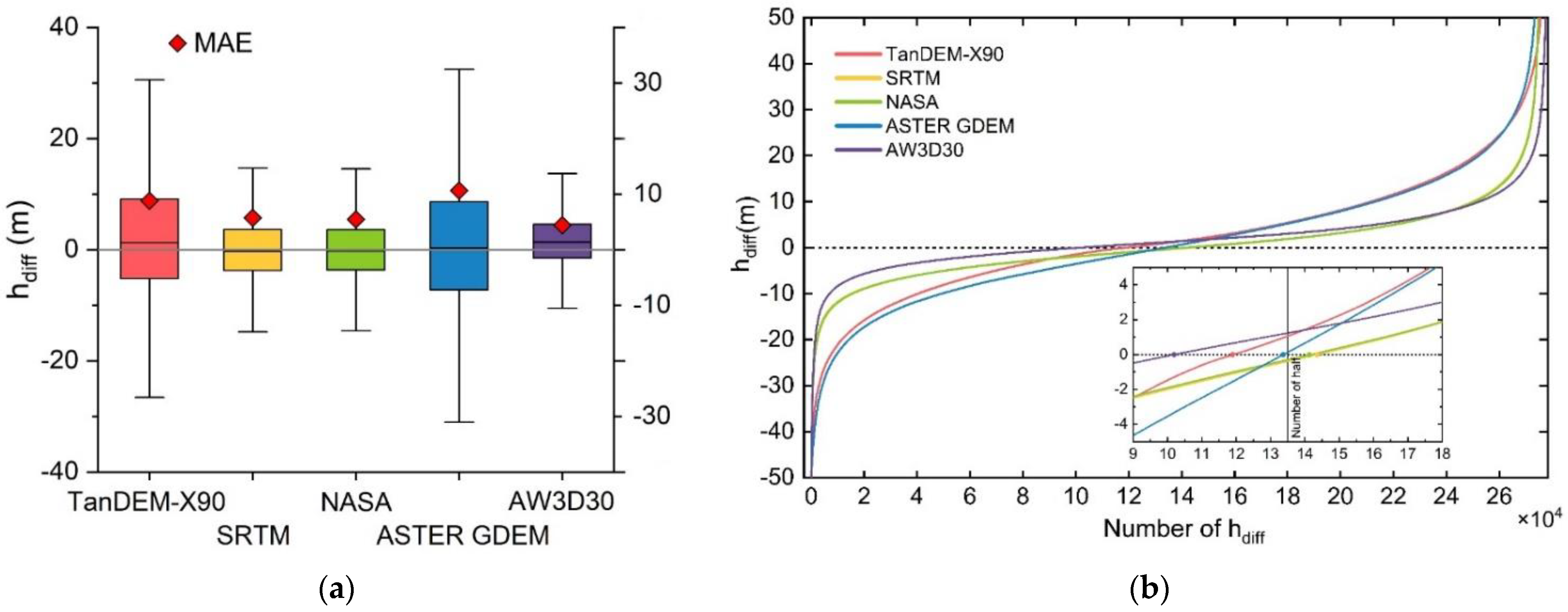
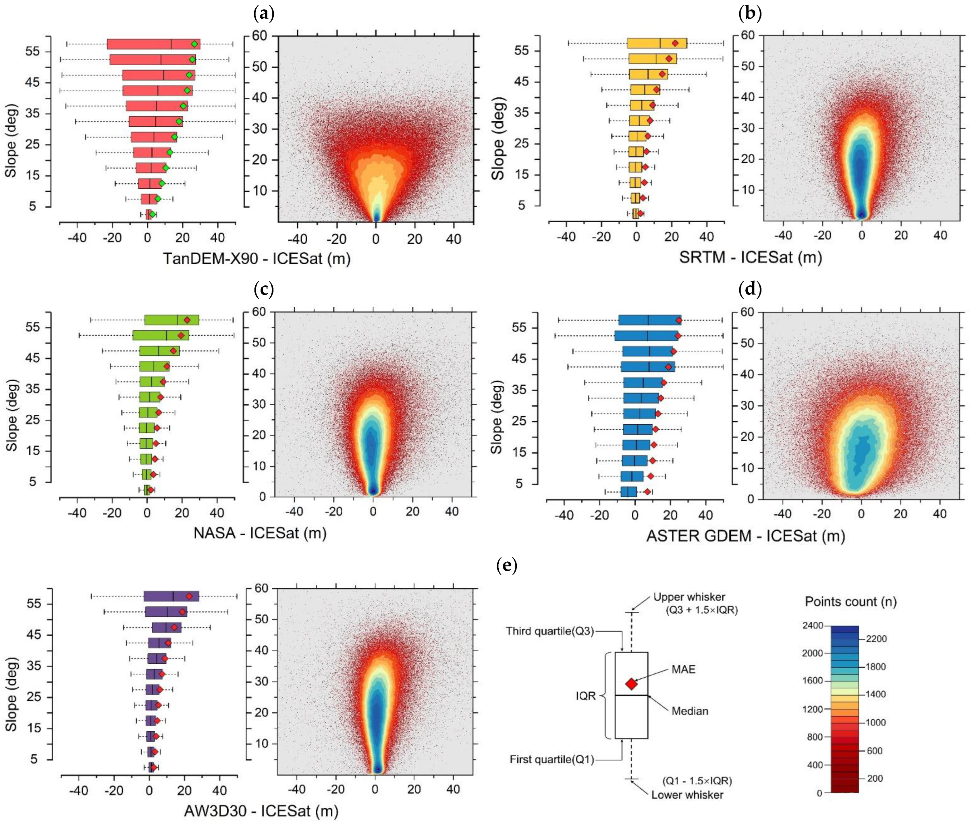
3.2. Quality Assessment of DEMs

The vertical accuracy of the DEMs can be quantized with elevation GCPs using the mean error (ME), standard deviation (STD), and root mean square error (RMSE) under the assumption that errors follow the Gaussian distribution [26]. However, the DEM error does not always follow the assumption of a normal distribution. This is not unique to us, as Nadi et al. [27] similarly found that DEM errors exhibit a slightly skewed normal distribution. Here, we demonstrate the normality of the height differences between ICESat/GLAS data and each DEM product using the Q-Q diagram in Figure 4.

The Q-Q plot (blue line) of each DEM product deviates from the graph of the ideal normal distribution (red line), indicating a non-normal distribution. Therefore, we use more robust indicators to evaluate the accuracy of a DEM that is not affected by outliers or skewed error distribution: median (MED), normalized median absolute deviation (NMAD), and mean absolute error (MAE) [26]. The definition of these indicators are as follows:

$$MED=media{n}_i\left\{(H_{\mathrm{DEM}}^i-H_{\mathrm{GLAS}}^i)\right\}=media{n}_i\left\{h_{\mathrm{diff}}^i\right\}$$

(1)

where $h_{\mathrm{diff}}^i$ is the elevation difference of the DEM products to be evaluated and ICESat/GLAS data on the ith sample. $median\left\{\right\}$ is to calculate the sample median, that is, to calculate the 50% quartile of the sample order statistics.

$$NMAD=1.4826\ast media{n}_i(|h_{\mathrm{diff}}^i-MED|)$$

(2)

NMAD represents the median of the absolute difference between the error and the median, which can be regarded as an estimate of STD with a heavy-tailed non-normal distribution. In the case of a normal distribution, this value is the same as the STD. When the number of sample points (n) is large enough, it can be considered a more flexible estimate of the STD for outliers in the dataset [26].

$$MAE=\frac{{\displaystyle {\sum }_{i=1}^m\left|h_{\mathrm{diff}}^i\right|}}{n}$$

(3)

MAE is a measurement of the average error. Unlike RMSE, it clearly measures the average error size [28]. The lower limit of RMSE is fixed at the MAE, and the upper limit tends to become larger with the increase $n^{1/2}$ and is easily affected by a small number of large errors.

3.3. Impact Factor Analysis with the Taguchi Model

In this study, the Taguchi model is introduced to evaluate the influence of different factors on DEM errors. The Taguchi model uses a tabular design (array) system to propose an experimental and statistical design based on multiple factors and levels. It allows the minimum number of experimental tests to study the impact of different factors on the mean and variance of the evaluation indicators and estimates the main effect of the maximum number of variables unbiasedly [29]. The Taguchi method introduced a signal-to-noise (S/N) ratio, which quantifies the impact of each factor on the research object from the response of evaluation indicators to noise factors and the signal factor ratio [30].

This study aims to explore the significance of terrain and surface factors in mountainous areas on DEM errors. Therefore, four levels of four factors, including landcover types, slope, FVCover, and aspect, are selected in the experimental design, as shown in

Table 2. Factors and Levels of Taguchi’s Experimental used in this study.

Factor	Description	Levels 1	Levels 2	Levels 3	Levels 4
A	GlobeLand30	cropland	forest	grassland	shrubland
B	Slope	0–10°	10–20°	20–30°	30–45°
C	FVCover	0–0.3	0.3–0.5	0.5–0.7	0.7–1
D	Aspect	north	east	south	west

. According to the conditions, the Taguchi experiment of the L16(4⁴) orthogonal array is designed. The maximum response level of each factor to the error-index is obtained by comparing the S/N ratio. The larger the S/N ratio is, the greater the influence of this combination of factors on the DEM error index. The S/N ratio is calculated by the following equation [31]:

This study explores the significance of terrain and surface factors in mountainous areas on DEM errors. Therefore, four levels of four factors, including landcover types, slope, FVCover and aspect, are selected in the experimental design, as shown in

Table 3. Quality indicators for the TanDEM-X90, SRTM, NASA, ASTER GDEM, and AW3D30 digital elevation models for the study areas.

DEM	MED (m)	NMAD (m)	MAE (m)	ME (m)	STD (m)	RMSE (m)
TanDEM-X90	0.97	10.54	9.76	1.21	13.12	13.30
SRTM	−0.28	5.41	5.45	0.44	8.01	8.03
NASA DEM	−0.19	5.37	5.41	0.42	7.97	7.98
ASTER GDEM	1.08	11.69	10.22	1.36	13.45	13.48
AW3D30	1.37	4.46	4.77	1.96	6.70	7.26

. According to the conditions, the Taguchi experiment of the L16(4⁴) orthogonal array is designed. The maximum response level of each factor to the error index is obtained by comparing the S/N ratio. The larger the S/N ratio is, the greater the influence of this combination of factors on the DEM error index. The S/N ratio is calculated by the following equation [31]:

$$\frac{S}{N}=-10Lo{g}_{10}\left(\frac{1}{n}{\displaystyle {\sum }_{i=1}^n\frac{1}{y_i^2}}\right)$$

(4)

where n is the number of repetitions of the same experiment and y is the measurement. Here, y is the MAE of the DEM under each different factor.

The analysis of variance (ANOVA) evaluates the relationship between each factor and the DEM error index according to the significance level statistics. The percentage contribution (P_C) of each factor to the change in the DEM error index is calculated by the following formula [32]:

$$P_C=\frac{S{S}_F-(DF\ast V_{Er})}{S{S}_T}\times 100$$

(5)

where SS_T is the sum of squares, SS_F is the sum of factorial squares, V_Er is the error variance, and DF is the degrees of freedom. DF, SS_T, SS and V_Er values are obtained from ANOVA.

4. Results

This section demonstrates the vertical accuracy evaluation of all five DEM products using the ICESat/GLAS data. The height differences between the DEMs and the ICESat/GLAS GCP data ($h_{\mathrm{diff}}$) were estimated. The boxplot in Figure 5a shows the overall quality of the five DEMs in the study area. The central horizontal line in the box marks the MED, and the red diamond represents MAE. It is found that the AW3D30 has the highest quality with the shortest interquartile distance and the smallest MAE. Figure 5b visualizes the distributions of the height difference ($h_{\mathrm{diff}}$). The distribution curve of $h_{\mathrm{diff}}$ is also the closest to zero. However, the MED of AW3D30 deviates the most in the positive value.

The indicators described in Section 3.2 are listed in Table 3. The MEDs of the SRTM and NASA DEMs are negative and very close to zero, while the MEDs of the other DEMs are positive. As a reprocessing product of the SRTM, NASA DEM is very similar to the SRTM and outperforms SRTM in all metrics. ASTER GDEM is the worst in almost all accuracy indicators, even worse than TanDEM-X90 with a 90-m resolution. The AW3D30 DEM showed the lowest NMAD (4.46 m) and MAE (4.77 m), indicating that it has the highest accuracy.

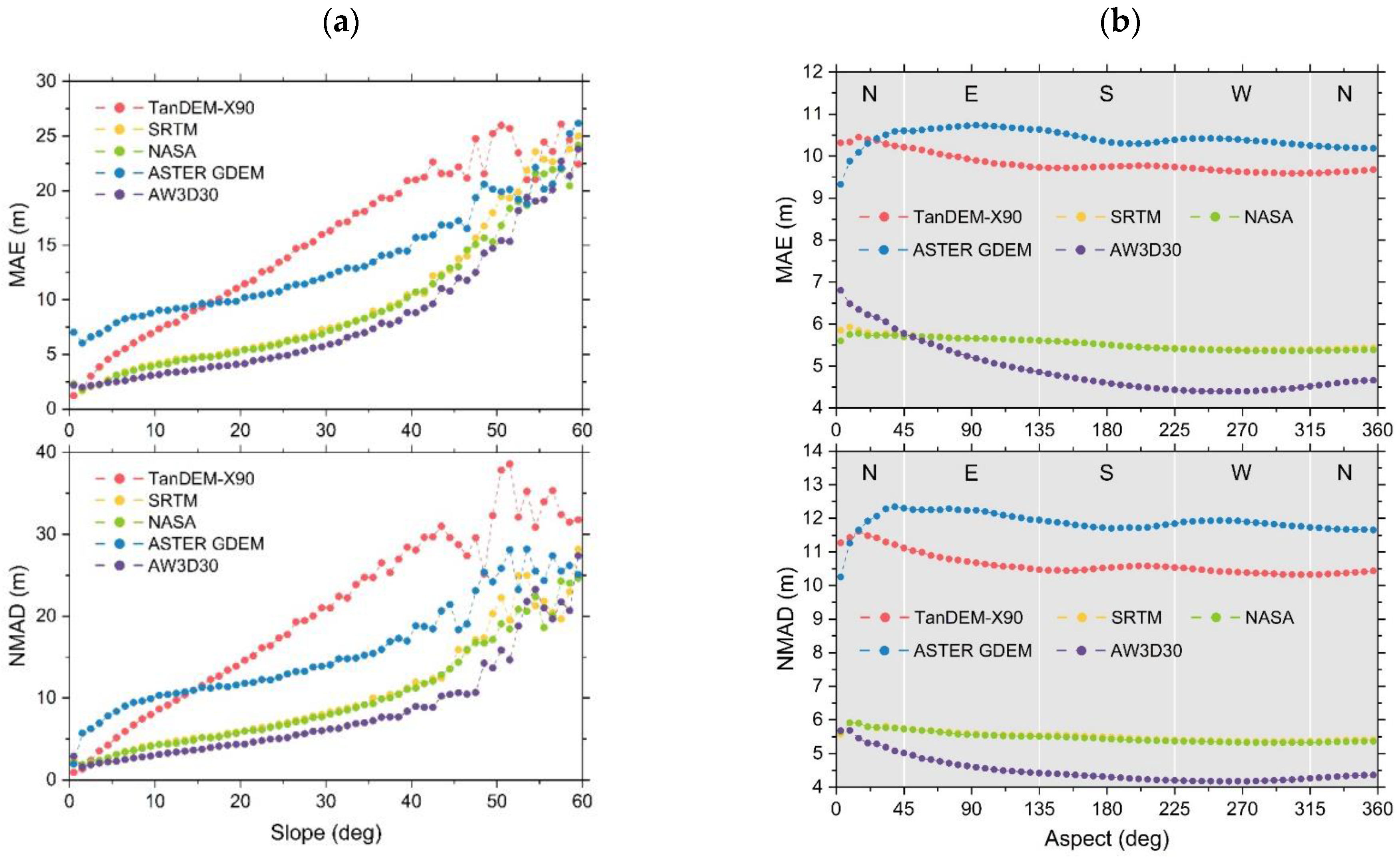
4.1. The Influence of Slope, Aspect, and Land Cover on DEM Accuracy

4.1.1. Influence of Slope and Aspect on DEM Accuracy

Figure 6 illustrates the variation of DEM error with slope. The box ranges and MAE of the radial box line graph increase with the slopes, indicating that the slope significantly impacts the vertical accuracy of all DEMs in the study area. Figure 6 also shows the hex-bin scatterplot of each DEM, which can better illustrate the error dispersion. The hex-bin scatter plot shows that the distribution of results of the TanDEM-X90 and ASTER GDEM are dispersed, and the ASTER GDEM and AW3D30 present obvious positive deviations with increased slopes.

The variation of DEM error with the slope aspect is described in Figure 7. Compared with the slope, the aspect has less impact on the DEM accuracy. The MAE of different DEMs fluctuates little with the change in the slope aspect. AW3D30 has the maximum error in the north direction, and ASTER GDEM has the worst accuracy in the southwest direction.

To better compare the consistency of DEM accuracy at different slopes and aspects, and to show the relationship between DEM accuracy and these two topographical features, we plotted scatters of different DEM accuracy indicators versus variation with slope (1° interval) and aspect (6° interval), as shown in Figure 8. The MAE of TanDEM-X90 varies the most with the slope, from 1 m at slope 0° to 26 m at slope 60°. The MAE of AW3D30 varies the most with the slope aspect, from 4.3 m at aspect 0° and 6.8 m at aspect 250°. The range of values of the MAE scatterplot represents to some extent the consistency of the DEM accuracy on the slope and slope up—the larger the range, the lower the consistency. AW3D30 shows the best consistency on the slope, while NASA DEM has the best consistency on the aspect. For another indicator NMAD, its value changes with slope and aspect with similar patterns.

MAE can be expressed as an increasing function of the slope. The MAE of TanDEM-X90 and ASTER GDEM is approximately linear with the slope, while the MAE of SRTM, NASA, and AW3D30 is approximately quadratic with the slope. When the slope is ≤2°, TanDEM-X90 provides the minimum MAE (1.2 m for slope ≤ 1° and 1.6 m for slope ≤ 2°). Unfortunately, MAE increases sharply with increasing slope. When the slope exceeds 15°, TanDEM-X90 has the largest MAE value among the five DEMs. Although the MAE of ASTER GDEM changes slowly, the overall error is relatively large. The MAE and NMAD of the other three DEMs increase slowly when the slope is ≤25°, and when the slope is >25°, the DEM accuracy decreases sharply with increasing slope.

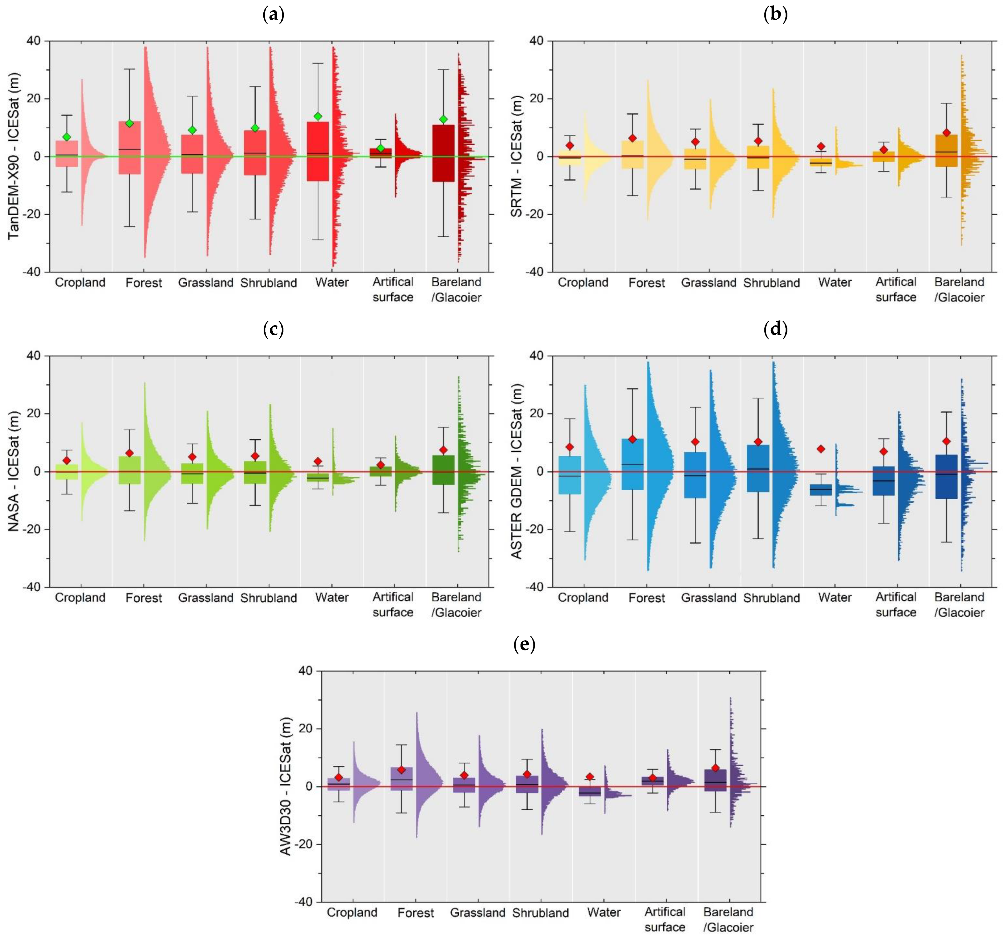
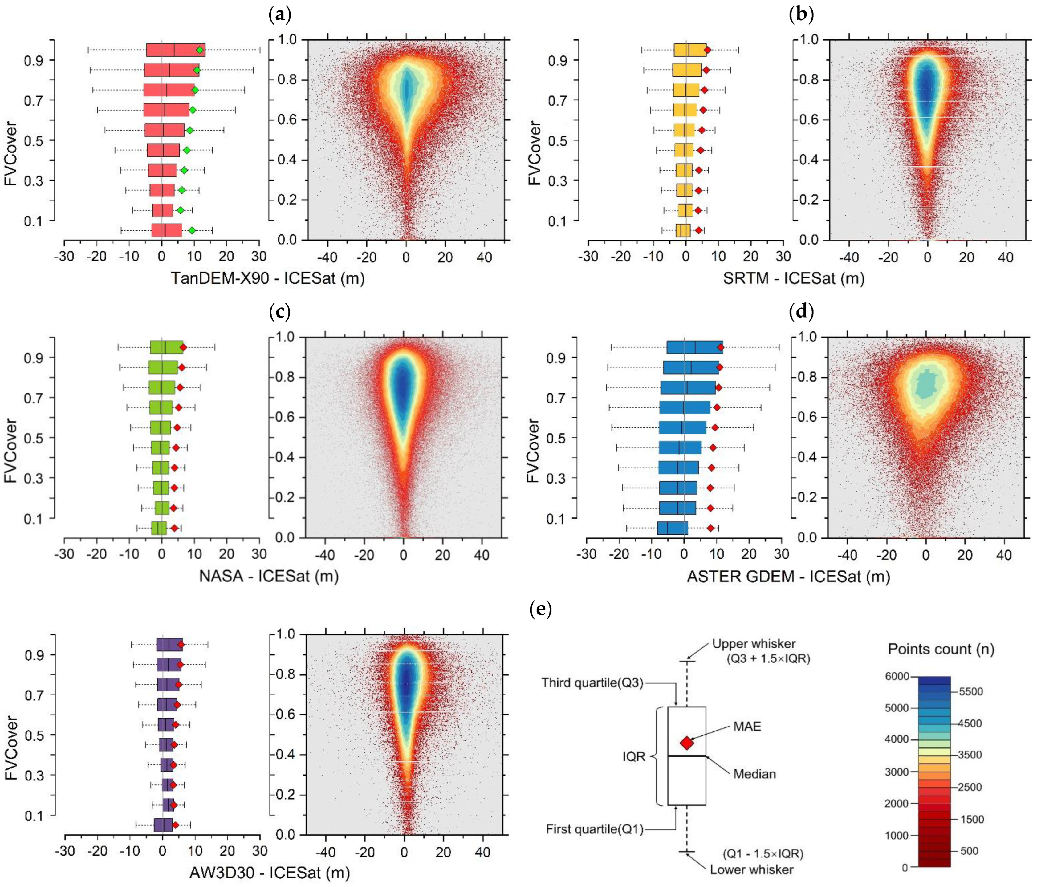
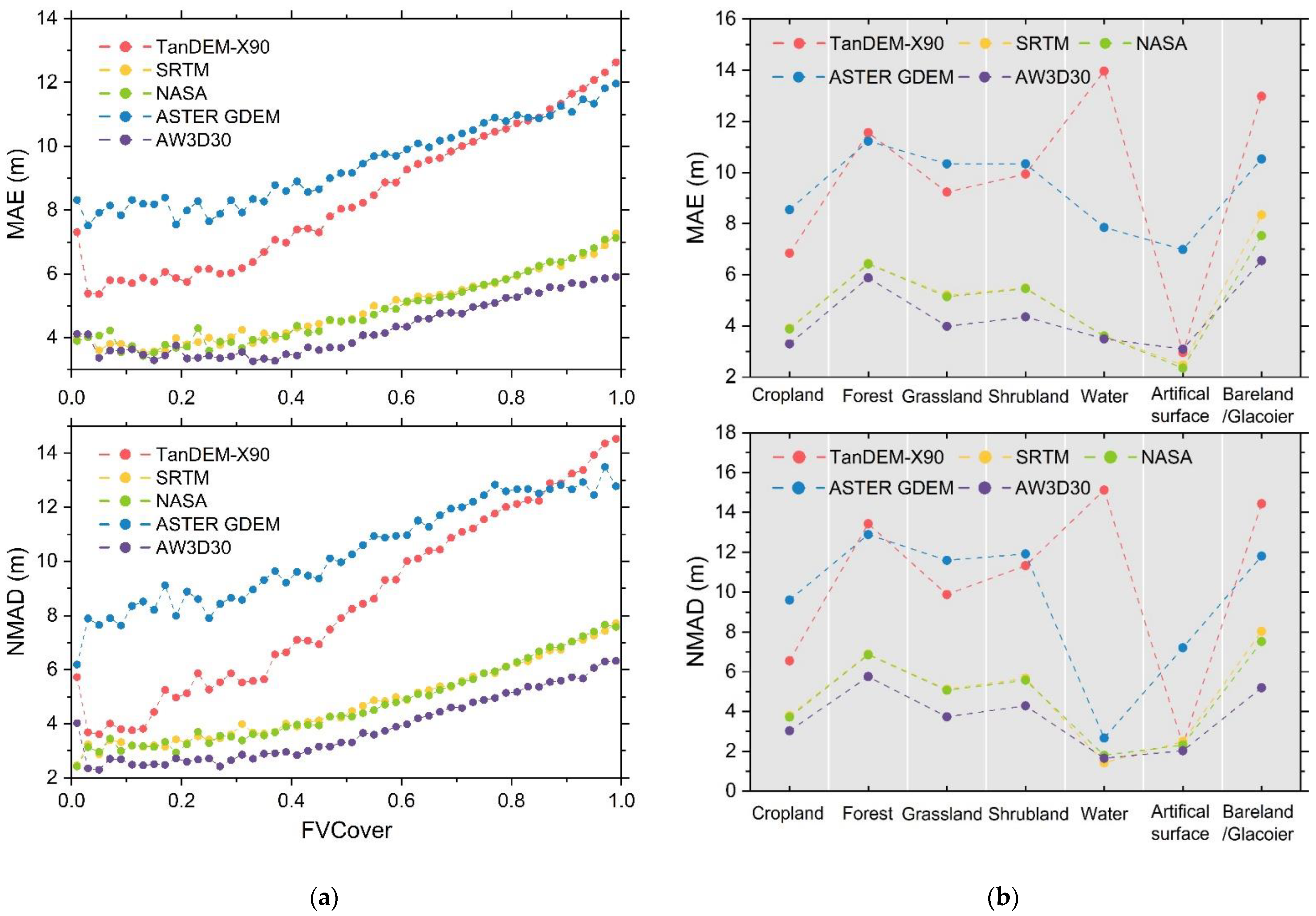
4.1.2. Influence of Landcover Types and Vegetation Coverage on DEM Accuracy

In this section, we compare the DEM errors in seven landcover types and depict the distribution of DEM errors in Figure 9. According to the error distribution, AW3D30 has the best quality in all landcover types, followed by NASA and SRTM, ASTER GDEM, and TanDEM-X. We found that all DEMs have the smallest MAE on the artificial surface. The MAE of all DEMs in the water body is inferior to that of the artificial surface, and their errors show negative deviation, except for the TanDEM-X DEM. In the vegetation-covered area, the MAE value of forest area is the largest, followed by shrubland, and the MAE value of grassland and cultivated land is the smallest. The elevation of all DEMs in forest areas is systematically higher than that of the actual surface. All DEM errors show higher MAE values in bare land/glacier areas. The error distribution is very discrete and deviates from the normal distribution, which will be explained in the next section.

Different vegetation sparsity under the same landcover types, that is, different vegetation coverages, will also cause changes in the phase center of reflected electromagnetic waves, resulting in significant differences in DEM errors [33]. Figure 10 shows the DEM errors vary with vegetation coverage. The box and hex-bin scatterplots show the DEM differences with FVCover. When 0 ≤ FVCover < 0.1, the MAE of these five DEMs has a high value. One explanation is that when the FVCover value is low, it includes glaciers/bare areas, increasing MAE. When 0.1 ≤ FVCover < 0.4, except for TanDEM-X90, the MAE values of the other DEMs remain stable and do not change with FVCover. When FVCover ≥ 0.4, the quality of all DEMs decreases slowly with increasing FVCover.

To reveal the consistency of DEM accuracy on different land cover types and vegetation cover, we introduced a dotted line map shown in Figure 11, with the range of variation of the same color as the dashed dotted line reflecting the consistency of DEM accuracy, and the larger the range of variation, the worse the consistency. The maximum change in MAE is over 10 m with the change in vegetation coverage (4 m for TanDEM-X90 FVCover 0.1 and more than 14 m for FVCover 1) and approximately 11 m with the change in landcover types (3 m for TanDEM-X90 in artificial surface area and 14 m in water body area). The maximum change in vegetation coverage in NMAD is approximately 11 m (4 m for TanDEM-X90 FVCover 0.1 and 15 m for FVCover 1), and the maximum change in landcover types is approximately 13 m (2 m for TanDEM-X90 artificial surface area and 15 m for water area). It can be seen that the MAE of TanDEM-X90 has the worst consistency in both vegetation cover and land cover types, and the same results are obtained in the NMAD index.

The impact of vegetation coverage on AW3D30 is the smallest (the variation range is approximately 3 m), followed by SRTM and NASA (the variation range is approximately 4 m). ASTER GDEM and TanDEM-X90 have higher MAEs at different FVCover values, showing the worst quality. ASTER GDEM and TanDEM-X90 have poor performance in different landcover areas, and in the non-water body and artificial surface areas, especially, their MAE values are far greater than those of the other three DEMs. However, it is worth noting that TanDEM-X90 has the same quality as AW3D30 in artificial surface areas. The quality indicators of the same DEM show obvious differences in different landcover areas, but these differences include errors caused by the different distributions of slope grades in different landcover types. Therefore, we further analyze the landcover types and slope together in Section 4.2.

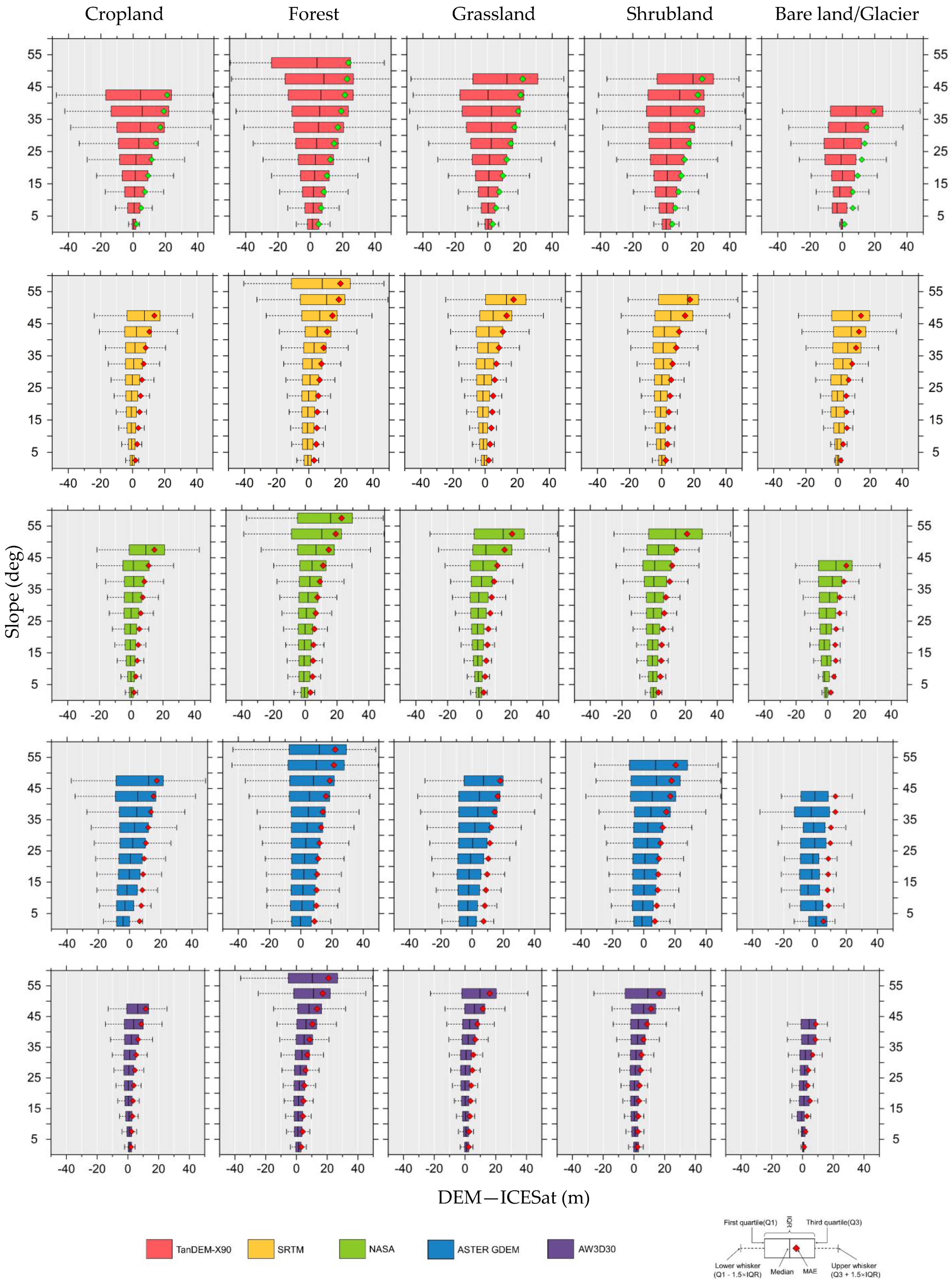
4.2. Significance Analysis of Slope Effect on DEM Quality after Excluding the Influence of Landcover Types

As discussed in Section 4.1, slope and landcover type are the two factors that affect the accuracy of the DEM the most. Figure 12 shows the distribution of the slope under different landcover types. The distribution of slopes is uneven in different landcover types, resulting in confounding the effect of the slope when analyzing the influence of varying landcover types on the MAE of DEMs. The slope range of the water body and artificial surface is the smallest, while the slope range in the glacier/bare land is the largest. The forest has the most significant slope in the vegetation-covered area, followed by shrubland and grassland, and arable land has the slightest slope. For further analysis, we introduced a box chart of landcover types grouped by slope, as shown in Figure 13, to perform slope analysis based on landcover types.

Figure 13 shows the variation of DEM errors with the slope in different landcover types. Since there is no obvious slope change in water bodies and artificial surface areas, we focus on the landcover types with mountainous areas. Thus, cropland, forest, grassland, shrubland, and bare land/glacier are selected to show the correlation between DEM errors and slopes of each landcover types. The boxplot and MAE of all landcover areas show high consistency with the slope change. The higher slope, the larger the MAE, except for glacier/bare land areas.

Figure 14 illustrates the quality indicators of DEM (MAE and NMAD) varying with the slope in different landcover types. The range of variation in MAE is also outlined in these four landcover types of cropland, forest, grassland, and shrubland in the same slope interval. AW3D30 shows the minimum error in each landcover type among all DEMs. SRTM and NASA have approximately the same mass for all coverage types. TanDEM-X90 offers good quality in the small slope area, but the quality decreases rapidly with the increasing slope. The ASTER GDEM has a significant error, even in flat areas. The MAE of the forest is slightly higher than that of the other three types of land cover, and the MAE of glacier/bare land fluctuates around the MAE of other types of land cover. The MAE differences between different land covers in the same slope are within 1.5 m, far less than the value of the differences between land covers calculated in Section 4.1.2, which confirms that slope is the main factor controlling the quality of the DEM. Another important point is that the consistency of DEM vertical accuracy is reflected in the MAE difference band in Figure 14. The wider the MAE difference band within the same slope interval, the worse the consistency of the representative quality across different land cover types. It can be seen that SRTM and NASA vertical accuracies have the best agreement across land cover types and AW3D30 has the worst agreement across land cover types.

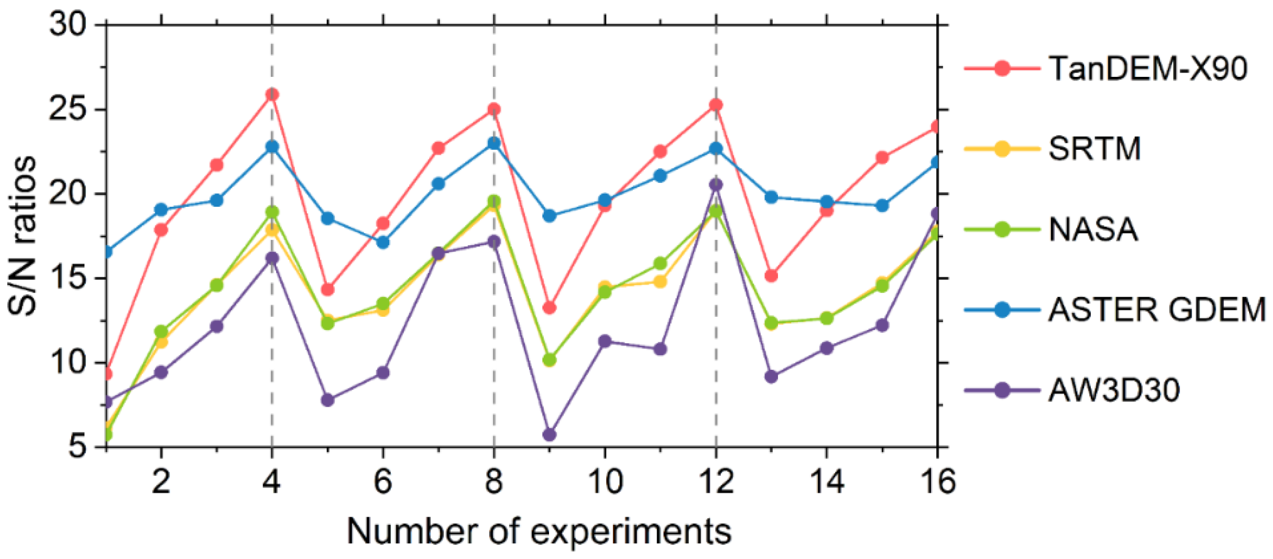
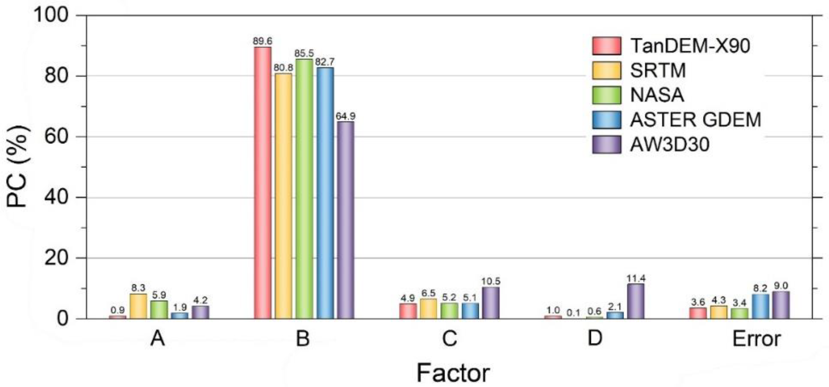
4.3. Quantitative Analysis of the Significance of Influencing Factors

Here, we developed a quantitative evaluation approach for exploring the impact of the slope, aspect, vegetation coverage, and landcover type on the accuracy of the DEM, as shown in

Table 4. Taguchi experimental conditions were used in this study.

NO.	L16 (Combination of Different Levels)				Influence Factor
					A	B	C	D
1	1	1	1	1	Cropland	0–10°	0–0.3	North
2	1	2	2	2		10–20°	0.3–0.5	East
3	1	3	3	3		20–30°	0.5–0.7	South
4	1	4	4	4		30–45°	0.7–1	West
5	2	1	2	3	Forest	0–10°	0.3–0.5	South
6	2	2	1	4		10–20°	0–0.3	West
7	2	3	4	1		20–30°	0.7–1	North
8	2	4	3	2		30–45°	0.5–0.7	East
9	3	1	3	4	Grassland	0–10°	0.5–0.7	West
10	3	2	4	3		10–20°	0.7–1	South
11	3	3	1	2		20–30°	0–0.3	East
12	3	4	2	1		30–45°	0.3–0.5	North
13	4	1	4	2	Shrubland	0–10°	0.7–1	East
14	4	2	3	1		10–20°	0.5–0.7	North
15	4	3	2	4		20–30°	0.3–0.5	West
16	4	4	1	3		30–45°	0–0.3	South

. We designed 16 experimental conditions and calculated the MAE values under different conditions. We could then determine the S/N ratio according to the equation (7).

Table 5. The results of Taguchi experiment, in which the S/N ratio of each experiment is generated by different combinations of factors and levels.

NO.	MAE (m)					S/N
	TanDEM-X90	SRTM	NASA	ASTER GDEM	AW3D30	TanDEM-X90	SRTM	NASA	ASTER GDEM	AW3D30
1	2.93	2.04	1.94	6.73	2.42	9.34	6.18	5.74	16.56	7.68
2	7.82	3.65	3.92	8.99	2.97	17.87	11.24	11.86	19.07	9.44
3	12.18	5.39	5.36	9.57	4.05	21.71	14.63	14.58	19.61	12.16
4	19.70	7.83	8.90	14.14	6.45	25.88	17.87	18.93	22.79	16.20
5	5.21	4.22	4.13	8.46	2.45	14.33	12.51	12.32	18.55	7.79
6	8.18	4.53	4.73	7.18	2.96	18.25	13.12	13.51	17.13	9.41
7	13.67	6.60	6.68	10.71	6.66	22.71	16.39	16.50	20.60	16.48
8	17.78	9.25	9.53	13.79	7.23	25.00	19.32	19.58	23.01	17.18
9	4.60	3.21	3.23	8.61	1.94	13.26	10.13	10.19	18.70	5.74
10	9.22	5.30	5.12	9.58	3.66	19.30	14.48	14.18	19.63	11.28
11	13.35	5.50	6.23	11.31	3.47	22.51	14.80	15.88	21.07	10.81
12	18.35	8.91	8.84	13.62	10.64	25.27	19.00	18.98	22.68	20.54
13	5.72	4.13	4.15	9.77	2.88	15.15	12.31	12.37	19.80	9.19
14	8.92	4.30	4.28	9.48	3.50	19.01	12.66	12.63	19.54	10.87
15	12.81	5.45	5.34	9.23	4.09	22.15	14.73	14.55	19.30	12.23
16	12.56	6.15	6.78	12.41	3.90	23.98	16.78	16.63	21.87	13.83

shows the impact on the MAE of factor combinations at different levels. The bold numbers in Table 5 refer to the maximum and second-largest signal-to-noise ratio values in the 16 experiments. These values are distributed in the factor level combination under the fourth-grade slope. The S/N maximum values of SRTM, NASA, and ASTER GDEM are obtained in the forest. Figure 15 shows that S/N fluctuates periodically in 16 experiments. The S/N ratio in low-slope areas is at wave troughs, and S/N values In high-slope areas are at wave peaks.

Table 6. The contribution to the DEM quality index MAE of each factor in the study area.

Factor	PC (%)
	TanDEM-X90	SRTM	NASADEM	ASTER GDEM	AW3D30
A (GlobaLand30)	0.9	8.3	5.9	1.9	4.2
B (slope)	89.3	80.8	85.0	82.7	64.9
C (FVCover)	4.9	6.5	5.2	5.1	10.5
D (aspect)	0.9	0.1	0.6	2.1	11.4
Error	3.6	4.3	3.4	8.2	9.0

and Figure 16 exhibit the percentage contribution of each factor to the MAE value of the DEM. Factor B (slope) has the largest contribution percentage among all DEMs. The contribution of the slope for TanDME-X90, SRTM, NASADEM, and ASTER GDEM is more than 80%. Even the lowest AW3D30 has 64%, showing that slope is the most significant factor affecting the quality of DEM. The other crucial factor is vegetation coverage. There are slight differences between the different DEMs. For SRTM and NASADEM, landcover type is more significant than vegetation coverage. For TanDEM-X90, SRTM, and NASADEM, the contribution of factor D (aspect) to the MAE is less than 1%, which can be almost ignored. For AW3D30, the contribution of the slope aspect is 11%, which cannot be ignored. For ASTER GDEM and AW3D30, produced using optical image data, the contribution percentage of error is significantly higher than that of SAR data. One reason is that optical satellite image data quality is more vulnerable to weather factors, which brings some inevitable errors.

5. Discussion

5.1. Penetration of Different Data

Different DEM data have diverse levels of penetration to the vegetation canopy due to different production methods, which can cause some errors. Figure 17 shows a schematic diagram of data penetration and the percentage of surface cover types corresponding to GCP points. The laser signal of ICESat/GLAS can partially penetrate the canopy through the gap between leaves, while the optical image cannot penetrate. Thus, the two DEMs generated from optical images, AW3D30 and ASTER GDEM, produce some overestimation due to the vegetation cover and have positive MED values. The TanDEM-X90 produced by X-band SAR images is also weak in penetrating vegetation, and its MED value is also positive. SRTM and NASADEM are mainly produced by C-band SAR images, which have a certain penetration. The data acquisition time is 5 years earlier than the average acquisition time of ICESat/GLAS data. The growth of plants may be the reason for the negative MED value.

It should be noted that the GCP points in forests and shrublands in the study area account for 70% of the total points, which makes the measurements of ICESat/GLAS larger than the actual DEM. However, it does not affect the relative accuracy of using ICESat/GLAS to compare different DEM products.

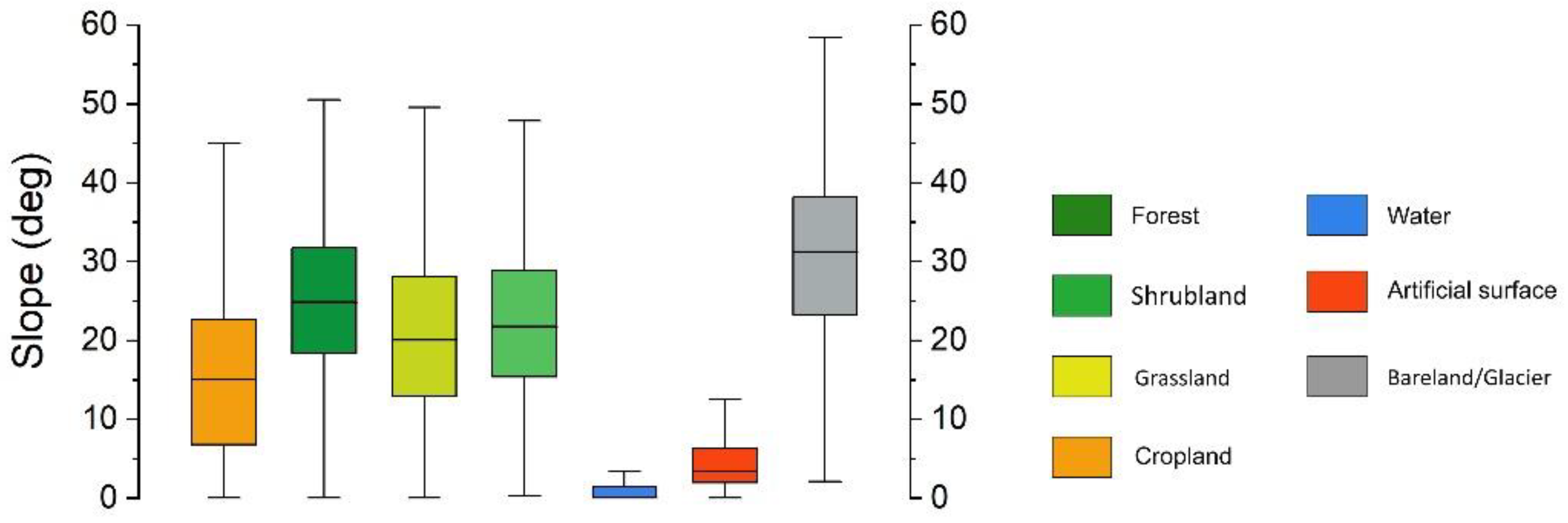
5.2. The Relationship between Landcover Types and DEM Quality

In Section 4.3, we conclude that slope is the most crucial factor affecting the DEM quality in complex mountain environments, followed by vegetation cover, while vertical accuracy is insensitive to both land cover and slope orientation. This is similar to the results of Nadi et al. [27], which show that the DEM errors are only directly related to the slope changes. However, Gdulová et al. [33] reported that landcover has a profound impact on the accuracy of TanDEM-X12 in the mountain environment of Europe. All DEMs have the worst consistency in terms of slope. As the distribution of slope varies considerably from region to region, some different but not contradictory results are obtained.

We changed the slope division in Table 3 with the division of the flat surface and calculated the contribution value of DEM accuracy, as shown in

Table 7. The contribution to the DEM quality index MAE of each factor in the flat area. (The parameters are the same as in Table 3 except for the slope. The slope is separated to 0–3°/3–6°/6–8°/8–10°).

Factor	PC (%)
	TanDEM-X90	SRTM	NASADEM	ASTER GDEM	AW3D30
A (GlobaLand30)	22.0	22.6	14.0	31.3	15.9
B (slope)	52.9	31.7	33.6	9.2	25.1
C (FVCover)	20.4	23.3	18.5	44.8	13.8
D (aspect)	2.5	20.8	25.1	1.8	23.7
Error	2.2	1.6	8.9	12.9	21.5
A + C	42.4	45.9	32.5	76.1	29.7

. The parameters except the slope are consistent with those used in the results of Table 6. We can find that the influence of vegetation and landcover has dramatically increased and is comparable to or even higher than the impact of the slope. The effect of vegetation and landcover types on ASTER GDEM errors in flat areas reaches 76% (Table 7), but only about 7% (Table 6) when all the slopes are considered. This also indicates, on the other hand, that the slope has a more significant effect on DEM accuracy than vegetation cover and surface type.

6. Conclusions

This study evaluates the accuracy of five globally covered and open-accessed DEM products (TanDEM-X90 m, SRTEM, NASADEM, ASTER GDEM, and AW3D30) in the mountain area in Southwest China. The processed high-precision ICESat/GLAS data are used as the elevation GCPs to validate the vertical accuracy of different DEM products. The robust evaluation indicators were utilized to compare the accuracy of the five DEMs and to explore the relationship between these errors and slope, aspect, landcover type, and vegetation coverage. The Taguchi method is introduced to quantify the impact of these surface characteristics on DEM errors.

The experimental results demonstrate that AW3D30 supplies the most robust and accurate DEM, followed by the NASADEM and SRTM. As a product reprocessed by SRTM, the accuracy of NASADEM has no noticeable improvement in MAE, except for the area with steep terrain (slope > 50°). TanDEM-X90 has the lowest MAE only on very flat terrain (slope < 2°) among these five DEM products, but its MAE increases shapely. When the slope exceeds 15°, TanDEM-X90 has the worse overall accuracy, while for the area with a slope < 15°, the accuracy of ASTER GDEM is the worst.

Among the factors that affect the accuracy of DEMs, the slope has the most significant influence, and the aspect has the least. Through the Taguchi experiment, it can be quantitatively calculated that the influence of the slope on DEM accuracy accounts for 90%, 81%, 85%, 83%, and 65% for TanDEM-X90, SRTM, NASADEM, ASTER GDEM, and AW3D30, respectively. While the influence of surface cover type only accounts for 1%, 8%, 6%, 2%, and 4% for these DEMs. This shows that the slope is the main factor affecting the accuracy of DEM in mountainous areas.

The surface types and vegetation cover also have significant influences on DEM accuracy, especially in the flat area. Among all types of land cover, the MAE of DEM in the artificial surface area is much smaller than that of other landcover types. NASADEM performs best among these five DEMs. In mountainous areas, the MAE of glaciers/bare land fluctuates greatly, which may be due to the terrain changes, such as snow cover and glacier melting. In areas with sparse vegetation (FVCover < 0.4), DEM accuracy is not sensitive to vegetation coverage change. In the dense vegetation-covered area, TanDEM-X90 was most affected by vegetation cover.

References

1. Wolock, D.M.; Price, C.V. Effects of digital elevation model map scale and data resolution on a topography-based watershed model. Water Resour. Res. 1994, 30, 3041–3052. [Google Scholar] [CrossRef]
2. Zink, M.; Bachmann, M.; Brautigam, B.; Fritz, T.; Hajnsek, I.; Moreira, A.; Wessel, B.; Krieger, G. TanDEM-X: The new global DEM takes shape. IEEE Geosci. Remote Sens. Mag. 2014, 2, 8–23. [Google Scholar] [CrossRef]
3. Farr, T.G.; Rosen, P.A.; Caro, E.; Crippen, R.; Duren, R.; Hensley, S.; Kobrick, M.; Paller, M.; Rodriguez, E.; Roth, L. The shuttle radar topography mission. Rev. Geophys. 2007, 45. [Google Scholar] [CrossRef] [Green Version]
4. Crippen, R.; Buckley, S.; Agram, P.; Belz, E.; Gurrola, E.; Hensley, S.; Kobrick, M.; Lavalle, M.; Martin, J.; Neumann, M. NASADEM global elevation model: Methods and progress. Int. Arch. Photogramm. Remote Sens. Spat. Inf. Sci. 2016, 41, 125–128. [Google Scholar] [CrossRef] [Green Version]
5. Tachikawa, T.; Hato, M.; Kaku, M.; Iwasaki, A. Characteristics of ASTER GDEM Version 2. In Proceedings of the International Geoscience and Remote Sensing Symposium, Vancouver, BC, Canada, 24–29 July 2011; pp. 3657–3660. [Google Scholar]
6. Takaku, J.; Tadono, T.; Doutsu, M.; Ohgushi, F.; Kai, H. Updates of ‘aw3d30’ alos global digital surface model with other open access datasets. Int. Arch. Photogramm. Remote Sens. Spat. Inf. Sci. 2020, 43, 183–189. [Google Scholar] [CrossRef]
7. del Rosario Gonzalez-Moradas, M.; Viveen, W. Evaluation of ASTER GDEM2, SRTMv3. 0, ALOS AW3D30 and TanDEM-X DEMs for the Peruvian Andes against highly accurate GNSS ground control points and geomorphological-hydrological metrics. Remote Sens. Environ. 2020, 237, 111509. [Google Scholar] [CrossRef]
8. Carrera-Hernandez, J.J. Not all DEMs are equal: An evaluation of six globally available 30 m resolution DEMs with geodetic benchmarks and LiDAR in Mexico. Remote Sens. Environ. 2021, 261, 112474. [Google Scholar] [CrossRef]
9. Podobnikar, T. Production of integrated digital terrain model from multiple datasets of different quality. Int. J. Geogr. Inf. Sci. 2005, 19, 69–89. [Google Scholar] [CrossRef]
10. Satgé, F.; Bonnet, M.-P.; Timouk, F.; Calmant, S.; Pillco, R.; Molina, J.; Lavado-Casimiro, W.; Arsen, A.; Crétaux, J.F.; Garnier, J. Accuracy assessment of SRTM v4 and ASTER GDEM v2 over the Altiplano watershed using ICESat/GLAS data. Int. J. Remote Sens. 2015, 36, 465–488. [Google Scholar] [CrossRef]
11. Hawker, L.; Neal, J.; Bates, P. Accuracy assessment of the TanDEM-X 90 Digital Elevation Model for selected floodplain sites. Remote Sens. Environ. 2019, 232, 111319. [Google Scholar] [CrossRef]
12. Yue, L.; Shen, H.; Zhang, L.; Zheng, X.; Zhang, F.; Yuan, Q. High-quality seamless DEM generation blending SRTM-1, ASTER GDEM v2 and ICESat/GLAS observations. ISPRS J. Photogramm. Remote Sens. 2017, 123, 20–34. [Google Scholar] [CrossRef] [Green Version]
13. Hu, M.; Ji, S. Accuracy evaluation and improvement of common DEM in Hubei Region based on ICESat/GLAS data. Earth Sci. Inform. 2021, 15, 221–231. [Google Scholar] [CrossRef]
14. Yap, L.; Kandé, L.H.; Nouayou, R.; Kamguia, J.; Ngouh, N.A.; Makuate, M.B. Vertical accuracy evaluation of freely available latest high-resolution (30 m) global digital elevation models over Cameroon (Central Africa) with GPS/leveling ground control points. Int. J. Digit. Earth 2019, 12, 500–524. [Google Scholar] [CrossRef]
15. Nardi, F.; Annis, A.; Di Baldassarre, G.; Vivoni, E.R.; Grimaldi, S. GFPLAIN250m, a global high-resolution dataset of Earth’s floodplains. Sci. Data 2019, 6, 180309. [Google Scholar] [CrossRef] [Green Version]
16. Rizzoli, P.; Martone, M.; Gonzalez, C.; Wecklich, C.; Tridon, D.B.; Bräutigam, B.; Bachmann, M.; Schulze, D.; Fritz, T.; Huber, M. Generation and performance assessment of the global TanDEM-X digital elevation model. ISPRS J. Photogramm. Remote Sens. 2017, 132, 119–139. [Google Scholar] [CrossRef] [Green Version]
17. Gesch, D.; Oimoen, M.; Danielson, J.; Meyer, D. Validation of the ASTER global digital elevation model version 3 over the conterminous United States. Int. Arch. Photogramm. Remote Sens. Spat. Inf. Sci. 2016, 41, 143. [Google Scholar] [CrossRef] [Green Version]
18. Tadono, T.; Nagai, H.; Ishida, H.; Oda, F.; Naito, S.; Minakawa, K.; Iwamoto, H. Generation of the 30 M-mesh global digital surface model by ALOS PRISM. Int. Arch. Photogramm. Remote Sens. Spat. Inf. Sci. 2016, 41. [Google Scholar] [CrossRef] [Green Version]
19. Li, H.; Zhao, J.; Yan, B.; Yue, L.; Wang, L. Global DEMs vary from one to another: An evaluation of newly released Copernicus, NASA and AW3D30 DEM on selected terrains of China using ICESat-2 altimetry data. Int. J. Digit. Earth 2022, 15, 1149–1168. [Google Scholar] [CrossRef]
20. Uuemaa, E.; Ahi, S.; Montibeller, B.; Muru, M.; Kmoch, A. Vertical accuracy of freely available global digital elevation models (ASTER, AW3D30, MERIT, TanDEM-X, SRTM, and NASADEM). Remote Sens. 2020, 12, 3482. [Google Scholar] [CrossRef]
21. Yamaguchi, Y.; Kahle, A.B.; Tsu, H.; Kawakami, T.; Pniel, M. Overview of advanced spaceborne thermal emission and reflection radiometer (ASTER). IEEE Trans. Geosci. Remote Sens. 1998, 36, 1062–1071. [Google Scholar] [CrossRef] [Green Version]
22. Abdallah, H.; Bailly, J.-S.; Baghdadi, N.; Lemarquand, N. Improving the assessment of ICESat water altimetry accuracy accounting for autocorrelation. ISPRS J. Photogramm. Remote Sens. 2011, 66, 833–844. [Google Scholar] [CrossRef] [Green Version]
23. Li, B.; Xie, H.; Tong, X.; Tang, H.; Liu, S.; Jin, Y.; Wang, C.; Ye, Z. High-Accuracy Laser Altimetry Global Elevation Control Point Dataset for Satellite Topographic Mapping. IEEE Trans. Geosci. Remote Sens. 2022, 60, 1–16. [Google Scholar] [CrossRef]
24. Chen, J.; Cao, X.; Peng, S.; Ren, H. Analysis and applications of GlobeLand30: A review. ISPRS Int. J. Geo-Inf. 2017, 6, 230. [Google Scholar] [CrossRef] [Green Version]
25. Gitelson, A.A.; Kaufman, Y.J.; Stark, R.; Rundquist, D. Novel algorithms for remote estimation of vegetation fraction. Remote Sens. Environ. 2002, 80, 76–87. [Google Scholar] [CrossRef] [Green Version]
26. Höhle, J.; Höhle, M. Accuracy assessment of digital elevation models by means of robust statistical methods. ISPRS J. Photogramm. Remote Sens. 2009, 64, 398–406. [Google Scholar] [CrossRef] [Green Version]
27. Nadi, S.; Shojaei, D.; Ghiasi, Y. Accuracy assessment of DEMs in different topographic complexity based on an optimum number of GCP formulation and error propagation analysis. J. Surv. Eng. 2020, 146, 04019019. [Google Scholar] [CrossRef]
28. Hodson, T.O. Root-mean-square error (RMSE) or mean absolute error (MAE): When to use them or not. Geosci. Model Dev. 2022, 15, 5481–5487. [Google Scholar] [CrossRef]
29. Taguchi, G. Quality engineering in Japan. Commun. Stat.-Theory Methods 1985, 14, 2785–2801. [Google Scholar] [CrossRef]
30. Freddi, A.; Salmon, M. Design Principles and Methodologies: From Conceptualization to First Prototyping with Examples and Case Studies; Springer: Berlin/Heidelberg, Germany, 2018. [Google Scholar]
31. Zhang, F.; Wang, M.; Yang, M. Successful application of the Taguchi method to simulated soil erosion experiments at the slope scale under various conditions. Catena 2021, 196, 104835. [Google Scholar] [CrossRef]
32. Sadeghi, S.H.; Moosavi, V.; Karami, A.; Behnia, N. Soil erosion assessment and prioritization of affecting factors at plot scale using the Taguchi method. J. Hydrol. 2012, 448, 174–180. [Google Scholar] [CrossRef]
33. Gdulová, K.; Marešová, J.; Moudrý, V. Accuracy assessment of the global TanDEM-X digital elevation model in a mountain environment. Remote Sens. Environ. 2020, 241, 111724. [Google Scholar] [CrossRef]
Figure 1. Study area: Yunnan Province, China. The colour changes on the graphic reflect changes in surface elevation, while the red dots indicate the ICESat satellite’s laser footprint on the ground.
Remotesensing 15 01952 g001
Figure 2. Schematic of DEMs comparison with ICESat/GLAS data.
Remotesensing 15 01952 g002
Figure 3. The distribution of the number of GCPs: (a) distribution on different elevations; (b) distribution on different slopes.
Remotesensing 15 01952 g003
Figure 4. The Q−Q diagram of the normality test of residuals.  h diff  is the height difference between the DEM products on top of the subfigures and the ICESat/GLAS data. The red line is the case of the ideal normal distribution. The blue line shows the actual situation of each DEM product.
Remotesensing 15 01952 g004
Figure 5. (a) Boxplot of five DEM products in the study area. (b) The error distributions of these five DEMs.
Remotesensing 15 01952 g005
Figure 6. The differences (i.e., bias) between five DEM products and ICESat/GLAS GCP points, shown as boxplots (with 5 degree intervals) and hex-bin scatterplots according to slope change: (a) TanDEM-X90, (b) SRTM, (c) NASA, (d) ASTER GDEM, (e) AW3D30.
Remotesensing 15 01952 g006
Figure 7. The differences (i.e., bias) between five DEM products and ICESat/GLAS GCP points, shown as boxplots (45 degree intervals) and hex-bin scatter plots according to aspect change: (a) TanDEM-X90, (b) SRTM, (c) NASA, (d) ASTER GDEM, and (e) AW3D30.
Remotesensing 15 01952 g007
Figure 8. Relationship between quality indicators ((top) MAE and (bottom) NMAD) and (a) slope and (b) aspect.
Remotesensing 15 01952 g008
Figure 9. The differences (i.e., bias) between five DEM products and ICESat/GLAS GCP points, shown boxplots and distribution histograms according to different landcover types: (a) Tan-DEM-X90, (b) SRTM, (c) NASA, (d) ASTER GDEM, and (e) AW3D30.
Remotesensing 15 01952 g009
Figure 10. The differences (i.e., bias) between five DEM products and ICESat GCP, shown as boxplots (with 0.1 intervals) and hex-bin scatter plots according to FVCover changes: (a) Tan-DEM-X, (b) SRTM, (c) NASA, (d) ASTER GDEM, and (e) AW3D30.
Remotesensing 15 01952 g010
Figure 11. Relationship between quality indicators ((top) MAE and (bottom) NMAD) and (a) FVCover (b) landcover types.
Remotesensing 15 01952 g011
Figure 12. Landcover and its relationship to slope.
Remotesensing 15 01952 g012
Figure 13. Slope-grouped boxplots of differences (i.e., bias) according to landcover types.
Remotesensing 15 01952 g013
Figure 14. Relationship between quality indicators (MAE on the top and NMAD on the bottom) and slope under different landcover types. (a) TanDEM-X90, (b) SRTM, (c) NASA, (d) ASTER GDEM, and (e) AW3D30.
Remotesensing 15 01952 g014
Figure 15. S/N of 16 experiments under different combinations of four factors.
Remotesensing 15 01952 g015
Figure 16. Percentage of contribution of each factor to MAE in the study area.
Remotesensing 15 01952 g016
Figure 17. (a) The left curve in the figure is the ICESat/GLAS echo waveform curve from the vegetation-covered flat ground, and the blue dotted line represents the actual position of the ICESat elevation point. The right side of the figure shows that the penetration of the DEM into the forest canopy is different due to the different wavelengths used by the sensors generating DEM products. The approximate depth of penetration is shown by the arrow. (b) The proportion of GCP points in different landcover types in the study area.
Remotesensing 15 01952 g017