A Novel Hybrid Intelligent SOPDEL Model with Comprehensive Data Preprocessing for Long-Time-Series Climate Prediction

Abstract

Long-time-series climate prediction is of great significance for mitigating disasters; promoting ecological civilization; identifying climate change patterns and preventing floods, drought and typhoons. However, the general public often struggles with the complexity and extensive temporal range of meteorological data when attempting to accurately forecast climate extremes. Sequence disorder, weak robustness, low characteristics and weak interpretability are four prevalent shortcomings in predicting long-time-series data. In order to resolve these deficiencies, our study gives a novel hybrid spatiotemporal model which offers comprehensive data preprocessing techniques, focusing on data decomposition, feature extraction and dimensionality upgrading. This model provides a feasible solution to the puzzling problem of long-term climate prediction. Firstly, we put forward a Period Division Region Segmentation Property Extraction (PD-RS-PE) approach, which divides the data into a stationary series (SS) for an Extreme Learning Machine (ELM) prediction and an oscillatory series (OS) for a Long Short-term Memory (LSTM) prediction to accommodate the changing trend of data sequences. Secondly, a new type of input-output mapping mode in a three-dimensional matrix was constructed to enhance the robustness of the prediction. Thirdly, we implemented a multi-layer technique to extract features of high-speed input data based on a Deep Belief Network (DBN) and Particle Swarm Optimization (PSO) for parameter searching of a neural network, thereby enhancing the overall system’s learning ability. Consequently, by integrating all the above innovative technologies, a novel hybrid SS-OS-PSO-DBN-ELM-LSTME (SOPDEL) model with comprehensive data preprocessing was established to improve the quality of long-time-series forecasting. Five models featuring partial enhancements are discussed in this paper and three state-of-the-art classical models were utilized for comparative experiments. The results demonstrated that the majority of evaluation indices exhibit a significant optimization in the proposed model. Additionally, a relevant evaluation system showed that the quality of “Excellent Prediction” and “Good Prediction” exceeds 90%, and no data with “Bad Prediction” appear, so the accuracy of the prediction process is obviously insured.

1. Introduction

The mitigation of climate change stands out as one of the most pressing challenges that humanity faces today. Climate change impacts can manifest in both positive and negative ways, but with the passage of time, the negative impacts have come to dominate. In different regions, the harmful impacts of climate change are observed in myriad forms, ranging from ecological disruption and declining biodiversity to soil erosion, dramatic temperature fluctuations, rising sea levels and global warming. Despite the intricacies involved in predicting the effects of climate change on Earth, there is a broad scientific consensus about its negative impacts [1,2]. Given the likelihood of long-term shifts in the global climate, an understanding of how precipitation and temperature may respond to changes in climatic conditions in the coming decades could be exceeding valuable [3]. This forms the key motivation for the present study.

There are several methodologies employed in climate prediction. We can categorize them into five mainstream types:

(1)

Empirical statistical method;

(2)

Mathematical statistical method;

(3)

Physical statistical method;

(4)

Dynamic mode;

(5)

Machine learning.

Next, we will describe the existing research results and characteristics of the above five methods in paragraphs.

Empirical statistical methods are based on identifying relevant patterns of atmospheric activity and climate change to predict corresponding outcomes [4]. Chryst et al. [5] proposed a method for calculating correlation coefficients by segments, which aims to address the presence of phases in the data and improve prediction accuracy. However, this approach is not without limitations, as it is only applicable to climate data with obvious periodicity or without complex relevancy.

Different from empirical statistical methods, mathematical statistical methods have gained widespread use in weather forecasting, demonstrating high accuracy and reliability that are highly dependent on the acquired data, which often follow data quality standards and quality measures [2]. Figura et al. [3] take advantage of linear regression models with historical groundwater and regional air temperature data to forecast the groundwater temperature in three aquifers by the end of the current century. Several other similar approaches can also be found in the literature [6,7,8,9].

In addition, a comparison and integration of two statistical methods have been explored to achieve higher accuracy in both regions [10]. In contrast to mathematical statistical methods, physical statistical methods entail a specific significance-based procedure to select factors. In particular, these methods rely on a system that characterizes the interconnectedness of atmospheric physical phenomena, from which the factors that meet the requirements for climate-influencing effects are selected. To further improve the predictive capacity of physical statistical methods, Cheng et al. [11] developed a conceptual model for the analysis of physical images with higher clarity. The ultimate results rely on the identification of certain factors chosen from an extensive set.

In spite of their usefulness, the aforementioned methods still face some challenges. Firstly, they require manual intervention to achieve good results based on human experience, and secondly, their ability to perform in complex situations is limited. To address these issues, the dynamic mode has emerged as an alternative approach based on understanding the locale-specific flow in the Atmospheric Boundary Layer (ABL) for both short-term and long-term predictions of atmospheric phenomena, such as the El Niño-Southern Oscillation (ENSO) and wind variability. Modes such as IAP-OGCM and CCM3 can predict future short-term climate change with promising results [12,13]. Meanwhile, computational fluid dynamics (CFD) is also becoming a preferred approach for climate prediction due to advances in computing hardware and software. However, most existing studies leveraging CFD have either considered idealized setups or a specific realistic situation while focusing on a limited number of climate variables [14].

Numerous Machine Learning (ML) techniques have been proven robust, reliable and efficient in dealing with sparse and multivariate climate datasets [15]. Support vector machines (SVMs) are mainly effective in predicting linearly separable data, albeit with limitations on general data influenced by the data size, parameters and kernel functions [16]. The increasing use of neural networks, which have stronger nonlinear mapping capabilities, has led to an uptick in climate data prediction. For example, back-propagation neural network algorithms have been employed to great effect in weather prediction [17]. Nonetheless, forecasting multi-dimensional time-series data such as climate change remains a challenging task due to inherent non-linearities and non-periodic behavior. Echo State Networks (ESNs), in contrast to other recurrent neural networks, are a promising option for online learning due to their lower requirements for training data and computational power [18]. A statistical time series forecasting technique can also be developed based on the autoregressive integrated moving average (ARIMA) model, which can generate annual projections by integrating recent observations with long-term historical trends [19]. Several other studies have also explored the use of neural networks in climate prediction. In [20], the authors paid attention to analyzing the hidden neurons in a back-propagation-feed forward neural network to identify the best pattern. Deshpande [21] took advantage of a Multilayer Perceptron Neural Network for multi-step ahead predictions of a rainfall data series and achieved optimal results in comparison with the Jordon Elmann Neural Network, Self-organized Feature Map (SOFM) and Recurrent Neural Network (RNN). Wu [22] considered enhancing prediction accuracy through both data-preprocessing techniques and modular modeling methods, with the ANN-SVR and MSVR outperforming other models in daily and monthly rainfall simulations. Some standards for network performance have also been researched. In terms of evaluating network performance, Gupta [23] compared different back-propagation network learning algorithms based on several criteria, such as correlation, root mean square error (RMSE) and standard deviation. In addition, previous research has studied intelligent algorithms such as the Extreme Learning Machine (ELM) for modeling extreme values in climate prediction. Real-time monitoring of water quality parameters is of utmost importance and, in this study, a new hybrid two-layer decomposition model coupled with an ELM and Least Square Support Vector Machine (LSSVM) was developed to improve the quality of this process. The model is based on a complete ensemble empirical mode decomposition algorithm with adaptive noise and a Variational Mode Decomposition (VMD) algorithm [24]. Another newly developed semi-supervised ELM framework with a k-means clustering algorithm for image segmentation and a co-training algorithm to enlarge the sample sets was used to classify agricultural planting structure in large-scale areas, with relatively fast training, good generalization, universal approximation capability and reasonable learning accuracy [25]. Furthermore, a Kernel Extreme Learning Machine (KELM) based on a Cell-Penetrating Peptide (CPP) prediction model was developed as an efficient prediction tool for identifying a unique CPP prior to experiments [26]. Due to the time-series nature of climate data, LSTM has been widely used in past prediction studies. To handle temperature data originating from body-mounted and fixed sensors, a warning mechanism for temperature increase was developed by combining a convolutional neural network (CNN) with LSTM. This mechanism exploits the contextualization ability of CNN-LSTM to predict temperature changes in windows of 5–120 s [27]. Multi-input single-output and multi-input multi-output strategies, namely LSTM-MISO and LSTM-MIMO, respectively, were carried out to predict accurate air temperature for multi-zone building based on direct multi-step prediction with a sequence-to-sequence approach [28]. The correlation between surface air temperature (SAT) and land surface temperature (LST) based on land use was analyzed using the TensorFlow LSTM [29]. To forecast the spatiotemporal variation of PM2.5, a hybrid model based on the deep learning method that integrates graph convolutional networks with Long Short-Term Memory networks (GC-LSTM) was proposed [30]. A deep learning-based method, namely the Transferred Bi-directional Long Short-term Memory (TL-BLSTM) model, was proposed for the prediction of air quality. This methodology framework utilizes a bi-directional LSTM model to learn from the long-term dependencies of PM2.5 and applies transfer learning to deliver knowledge learned from smaller temporal resolutions to larger temporal resolutions [31]. LSTM-based deep neural networks with self-organizing feature maps were adopted to achieve high-spatial-resolution sea surface temperature prediction [32].

Notwithstanding the effectiveness of the extant climate prediction methods, they primarily concentrate on short-term forecasting. Given the inherent instability and volatility of climate data, even the most refined and extensive climate model may suffer from distortions when forecasting for longer periods. Specifically, despite the extensive use of intelligent models in climate prediction, there are still several challenges that need to be addressed, mainly including: (1) the current prediction method for climate data of the same category lacks delicate data classification based on different time orders, which results in sequence disorder; (2) there is a lack of effective methods to expand the dimensions of training data to strengthen the robustness of the model; (3) a significant amount of input data is often useless, which increases the difficulty in extracting characteristic data; (4) the lack of optimized initial data hinders the interpretation of the model. As a consequence of these defects, the focus of climate prediction has been mainly on short time series, leading to shortcomings in the output of long time series. For the former three challenges, we can conclude that adequate data preprocessing work is essential for the prediction of long-term data. It contains three parts in this paper: dataset decomposition, feature extraction and input conversion. For the latter, we can carry out an optimization model utilized for the parameters in a neural network.

For dataset decomposition, to achieve high-precision forecasting, the proposed model leverages two neural network algorithms with a novel decomposition approach for raw data. The combination of these two features endows the proposed system with the ability to make accurate long-term climate predictions.

For feature extraction, obtaining the most valuable information from long-term useful data during the data training process is still a challenge. This paper proposed a combination of a Deep Belief Network (DBN) with ELM and LSTM to assign the characteristic data of DBN training to neural networks for calling more valuable information and improving the accuracy of climate prediction.

For input conversion, during time-series prediction, it is common to employ the independent variable from the previous time to directly predict the dependent variable of the future time using a linear-type input mode. A “rolling window” method is typically utilized for data preprocessing in order to enhance the accuracy of air quality prediction. Despite these efforts, the linear-type input mode persists. Therefore, this paper proposes a novel approach utilizing a body-type input to a linear-type output mapping pattern. Compared to the previous model, the model of our study achieves a substantial improvement in prediction accuracy.

Moreover, for the optimization of parameters in a neural network, theoretically, the improvement of ELM and LSTM’s training accuracy depends not only on a larger number of hidden nodes but also on more appropriate initial values. To improve the quality and accuracy of the prediction, this study utilized Particle Swarm Optimization (PSO) to optimize ELM and LSTM to obtain the optimal initial threshold and weight.

To sum up, this paper stressed a novel hybrid spatiotemporal system for long-term climate prediction. By using this model, decision makers and non-professionals can make more accurate judgments and assessments of climate change in the future, climate analysts can also use this as a means of analyzing long-term climate data to gain further insight into the trends of global and local climate change in different periods. This system includes a novel optimal-hybrid model called SS-OS-PSO-DBN-ELM-LSTME (SOPDEL) that integrates machine learning, an optimization algorithm, input-output remapping, feature extraction and data decomposition. Machine learning techniques used in the model include ELM and LSTM neural networks, while the optimization algorithm is based on PSO. Input-output remapping is achieved through a three-dimensional input conversion technology in a novel spatiotemporal-factor matrix, and feature extraction uses a DBN as preprocessing for machine learning. Data decomposition employs a novel PD-RS-PE technology. To validate the accuracy and stability of the proposed model, five models featuring partial enhancements were discussed in this paper and three state-of-the-art classical models were utilized for comparative experiments. The results showed that SOPDEL outperformed the other models, improving four evaluation indices compared with traditional LSTM prediction and reducing the cumulative error of long-time-series prediction. Moreover, the proposed model’s excellent rate is attributed to the development of an evolution index system of climate prediction.

The main contributions and innovations of this paper are as follows: (1) A novel optimal-hybrid model named SOPDEL was established, which integrates machine learning, optimization algorithm, input-output remapping, feature extraction and data decomposition. This model represents a notable improvement in the forecasting quality of climate data. (2) PD-RS-PE technology was proposed, which effectively divides data into a stationary series (SS) and oscillatory series (OS), allowing for the use of both smooth-predicting characteristics of LSTM and extreme-predicting characteristics of ELM to improve the accuracy of prediction. (3) A new type of input-output mapping mode was constructed using a three-dimensional matrix composed of region, month and climate impact factors. In this matrix, a shape-input-mapping linear output was employed to extract original climate data step by step, which enhances the robustness of the prediction. (4) A method to extract features of input data from ELM and LSTM was proposed, which enhances the learning ability of the prediction system. In conclusion, our approach addresses key challenges such as sequence disorder, weak robustness, low characteristics and weak interpretability to achieve long-time-series climate prediction. The findings have important implications for policymakers, urging them to promulgate relevant decisions to control the impacts of climate change. Furthermore, our methods have significant potential for application to other long-time-series data due to their stability and extensibility in processing oscillatory series.

2. Materials and Methods

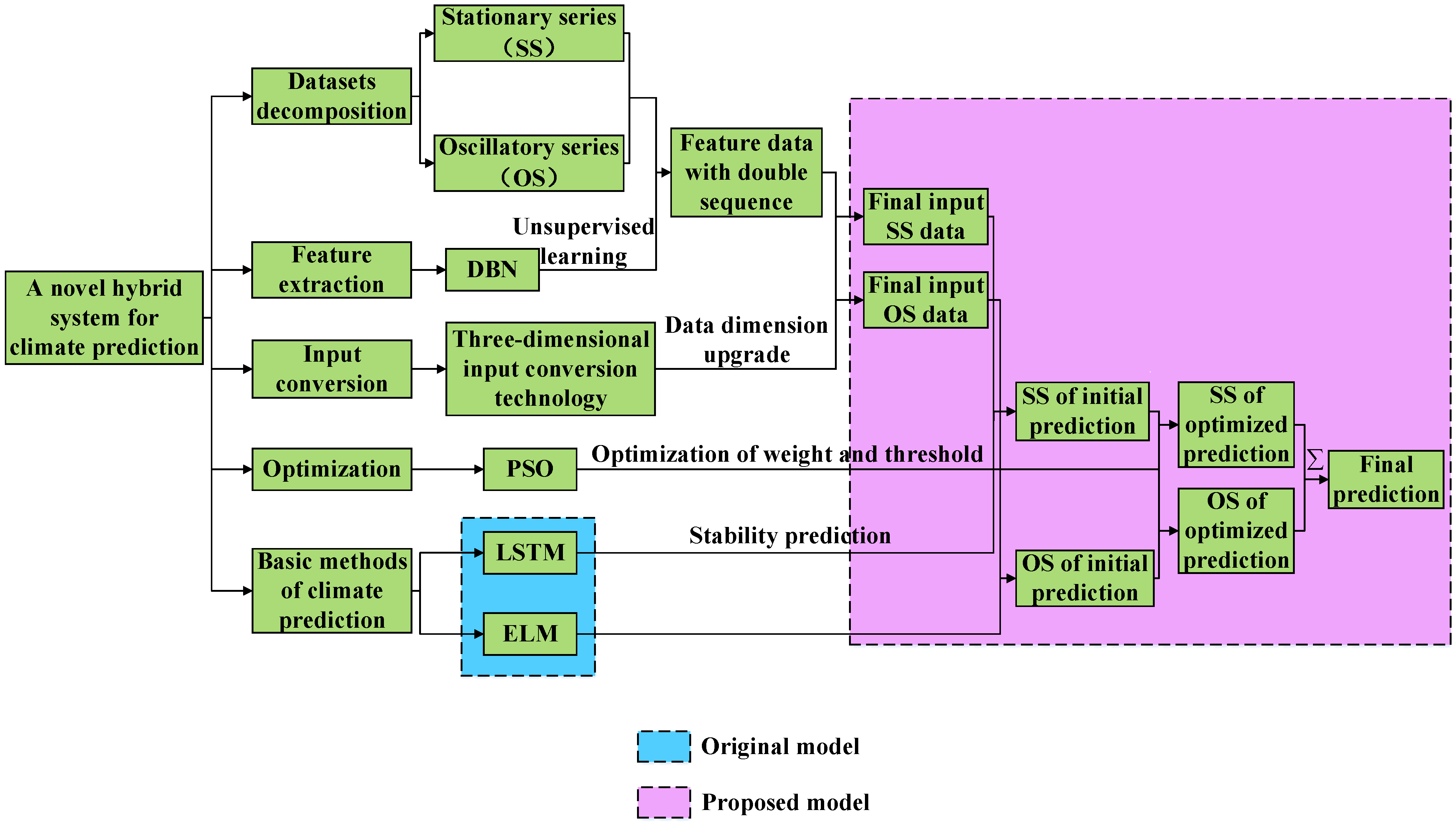
2.1. General Idea of This Paper

An overall flow chart of this paper is shown in Figure 1, and the process of the proposed SOPDEL model is shown in Figure 2. It mainly includes five parts: datasets decomposition, feature extraction, input conversion, optimization and final prediction through machine learning. The proposed improvements to the intelligent prediction algorithm are twofold: (1) the original data were decomposed, feature-extracted and dimension-remapped to be well qualified for neural network training; (2) the weights and thresholds of the neural network model were optimized to improve the convergence speed. The above-mentioned enhancements aim to improve the model’s suitability for comprehensiveness and stability prediction of climate data with long periodicity and oscillation. The study’s findings suggest that the SOPDEL model is well suited for climate prediction processes and can significantly improve their performance.

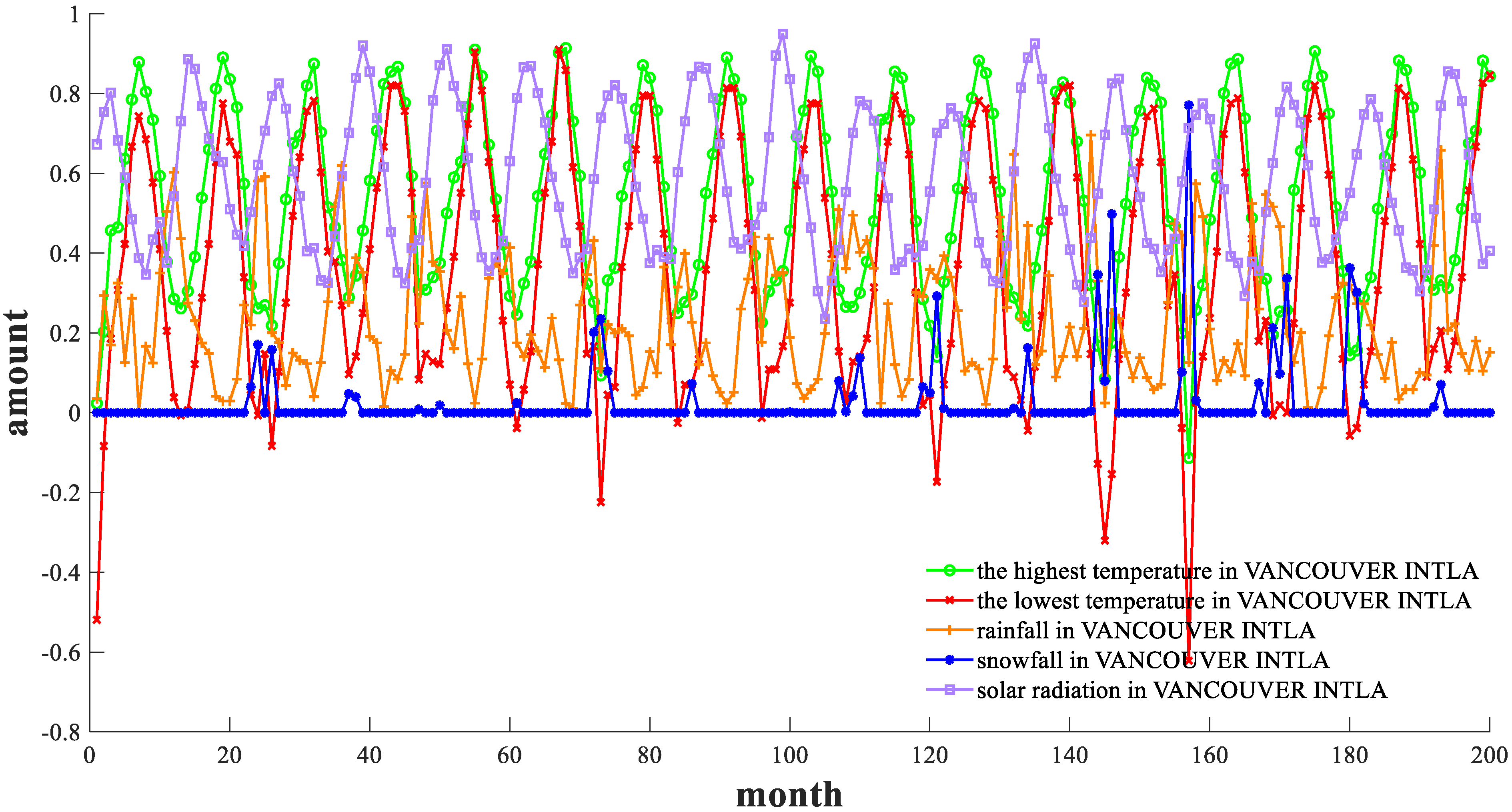
2.2. Data Acquisition by Remote Sensing

This study utilizes remote sensing techniques to collect climate data, including temperature, rainfall and snowfall, for the raw materials of developing a machine-learning model. The amount of solar radiation is measured using a pyranometer or sunshine meter.

(1)

Temperature obtained by remote sensing: The meteorological satellite is equipped with a remote sensor that captures sensing images, while a sensing instrument performs inversion by measuring the range of thermal radiation. Various sensors are employed to observe far-infrared bands and obtain pixel values, as different components of the earth’s surface exhibit different radiation characteristics along bands. The values are then converted into thermal infrared radiation values, and an appropriate mapping is established between radiation values and the earth’s surface temperature by using suitable models.

(2)

Rainfall obtained by remote sensing: The method can be divided into infrared remote sensing, passive-microwave remote sensing and active-microwave detection. Infrared remote sensing retrieves surface precipitation intensity by utilizing the empirical relationship between the cloud-top temperature and surface precipitation. Generally, strong-precipitation clouds tend to have a lower cloud-top temperature. The widely-used satellite-infrared-inversing precipitation data were developed by the prediction center of the Atmospheric and Oceanic Administration of the United States according to this principle. A GPI algorithm is more suitable for deep convective precipitation and has poor expressiveness for stratus precipitation. Passive microwave remote sensing employs two schemes for retrieving precipitation: the microwave-emission scheme and the scattering scheme. The microwave-emission scheme inverts the surface precipitation by observing low-frequency (e.g., 19 GHz) microwave radiation emitted by precipitation particles. The principle behind the scheme is that, under the lower radiation background, stronger precipitation and more liquid water particles in the cloud will increase the brightness temperature of upward radiation. This scheme has demonstrated good results on the ocean surface but not on land. In contrast, the microwave scattering scheme retrieves precipitation by utilizing a high-frequency (e.g., 85 ghz) signal of ice particles on the upper part of the cloud. The more ice particles there are, the lower the upward-scattering-brightness temperature and the stronger the surface precipitation. Although the microwave scattering scheme is more indirect compared with the emission scheme, it can be used to invert land-surface precipitation by establishing an empirical or semi-empirical relationship between the precipitation rate and scattering signal according to the observation.

(3)

Snowfall obtained by remote sensing: The method used is the same as that of measuring rainfall. Raining or snowing is related to local temperature.

In the present study, VANCOUVER INT’L A, located in the southwestern region of Canada, was chosen as the study area. The data used in the investigation were obtained by applying the aforementioned methodology with monthly records of the highest temperature, the lowest temperature, solar radiation, rainfall and snowfall from 1937 to 2020. To facilitate the comparative analysis, the collected data were normalized, and the former 200 datasets are presented in Figure 3. These six key factors are considered to have a significant impact on climate prediction.

2.3. PD-RS-PE Technology for Data Decomposition

Obviously, the performance of intelligent algorithms varies with different input sequences. Thus, it is crucial to decompose climate data with respect to time coordinates, which is referred to as “data decomposition”. In climate data, the wave crests and troughs exhibit distinct changes, while the intermediate values remain relatively stable. Therefore, separating the peak and valley values at both ends from the intermediate values can aid in separating climate data according to their distinct properties. This novel approach is called “PD-RS-PE technology” (refer to Algorithm 1).

Algorithm 1. PD-RS-PE.

Input: original climate data $HT,LT,RF$

Output: decomposed climate data $SS–HT,OS–HT,SS–LT,OS–LT,SS–RF,OS–RF$

1.        construct three figures with x-axis of month and y-axis of $HT,LT,RF$ respectively

2.        for each period of input do in figures

3.        split variables with 12 sub-coordinates to $n$ sub region

4.        end for

5.        for each sub region do in figures

6.        get minimum value in peaks $pe{a}_{\min 1},pe{a}_{\min 2},\cdots pe{a}_{\min n}$

7.        get maximum value in valleys $va{l}_{\max 1},va{l}_{\max 2},\cdots ,va{l}_{\max n}$

8.        end for

9.        get $pe{a}_{\min }=\min (pe{a}_{\min 1},pe{a}_{\min 2},\cdots pe{a}_{\min n})$

10.      get $va{l}_{\max }=\max (va{l}_{\max 1},va{l}_{\max 2},\cdots ,va{l}_{\max n})$

11.      draw a line $l_1$ crossing $pe{a}_{\min }$ and perpendicular to y-axis

12.      draw a line $l_2$ crossing $va{l}_{\max }$ and perpendicular to y-axis

13.      extract data with $\begin{array}{ccccccccc}lower& to& l_1& and& upper& to& l_2& \to & SS\end{array}$, $\begin{array}{ccccccccc}upper& to& l_1& and& lower& to& l_2& \to & OS\end{array}$

The forecasting of stationary and oscillatory time series data by various neural networks can yield distinct outcomes. Given that climate data exhibit both types of series, the need for a data decomposition approach arises. The proposed method involves partitioning the data based on peak, valley, and intermediate values, resulting in the PD-RS-PE technology. Subsequently, a combination of neural networks can be used to forecast climate data, utilizing the specific properties of each network.

The steps are mainly divided into three steps:

Step 1: Take every 12 months as a period to describe the chart of the highest temperature, lowest temperature and rainfall. The area behind each section is labeled as $v_1,v_2,\cdots ,v_n$. This segmentation of the chart into discrete periods is termed period division (PD).

Step 2: In each sub-region, the dependent variable’s peak and valley values are identified, and the minimum peak and maximum valley points are extracted. A straight line is drawn between these two points perpendicular to the $y$ axis, divide this chart into the first sub-region composed of middle the part, recorded as $p_1$, and the second horizontal sub-region composed of the upper and lower parts, recorded as $p_2$. This process is called region segmentation (RS).

Step 3: The proposed method involves extracting data from two distinct regions, namely, $p_1$ and $p_2$, which are then transformed into a stationary series (SS) and oscillatory series (OS), respectively. Since these two types of data possess different properties, they can be forecasted using different methods. This step is referred to as property extraction (PE).

A flow chart of the proposed data extraction method is shown in Figure 4.

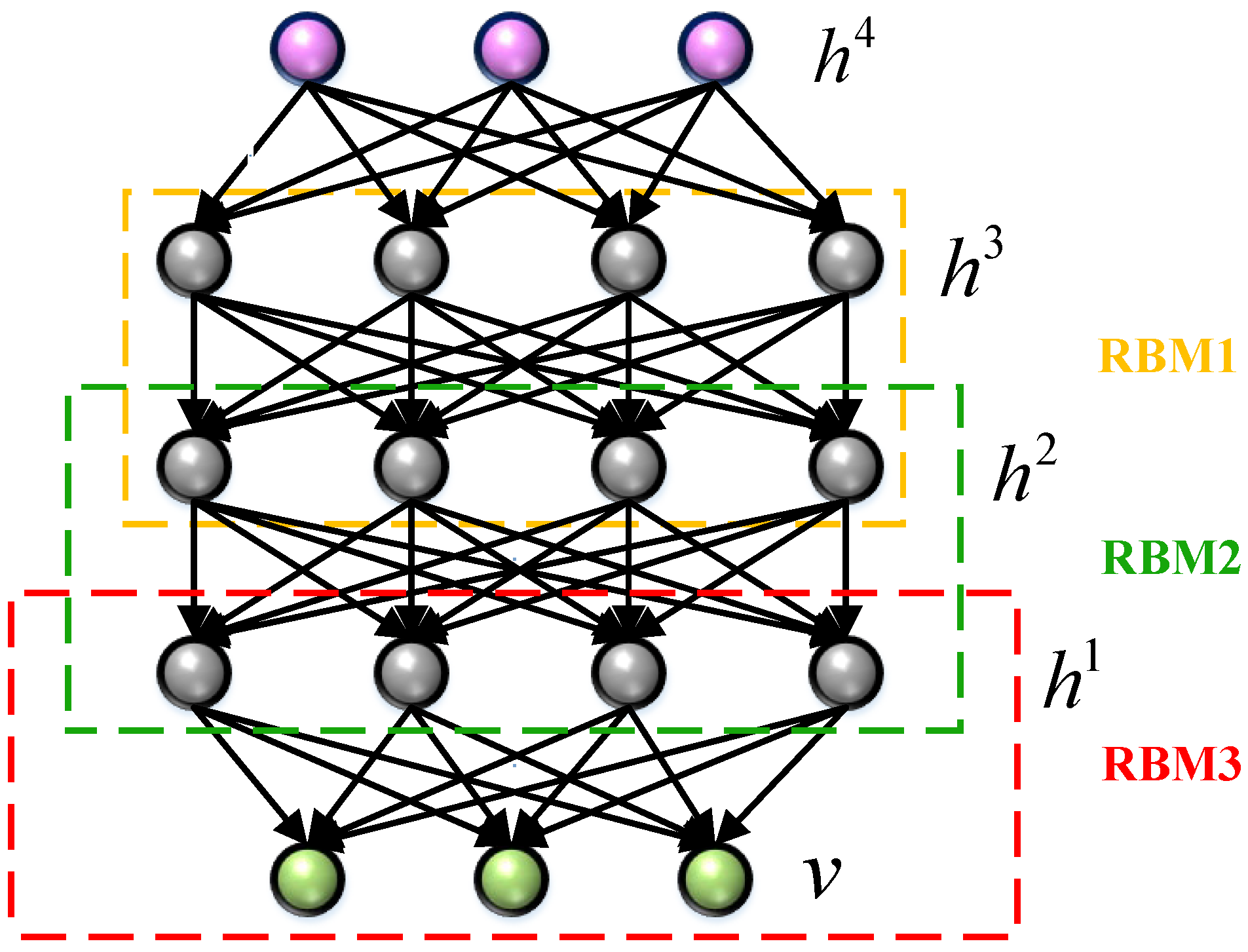
2.4. Unsupervised Learning for Feature Extraction

The information contained in the input data for neural network prediction is often redundant, leading to a long training time and overfitting. To mitigate this issue, the proposed method of “feature extraction” is introduced to extract useful information from the input data. A Deep Belief Network (DBN) was chosen as the feature extraction method due to its strong capacity for processing unlabeled data, which is the category that climate data belong. Compared to other dimensionality reduction algorithms such as the PCA, the DBN has a better performance, allowing it to effectively extract internal characteristics from high-dimensional climate data that are affected by complex conditions.

The DBN is a neural network composed of a series of Restricted Boltzmann Machines (RBMs), which are a type of neural perceptron. Unlike ordinary Boltzmann Machines, RBMs have a simplified internal connection form with no connection within the hidden layer, thereby greatly reducing computation [33,34]. This means that the activation of each hidden layer unit is independent when the visible layer unit state (input data) is given. Similarly, activated conditions of each visible layer unit are also independent when the state of the hidden layer unit is given, which allows for more efficient processing of high-dimensional data.

In the context of a DBN, the input data are fed into the network through lower-level RBMs, and the network output is obtained by a layer-to-layer forward computation. The network training process is different from conventional artificial neural network training. During the pre-training stage, each RBM is trained separately from a lower level, with the objective of minimizing the network energy. After the training of a lower-level RBM is completed, the output of its hidden layer is used as the input of the next higher-level RBM, which is then trained. This layer-by-layer training process continues until all RBMs have been trained. It is noteworthy that only the input data is used in the pre-training process without a label, rendering a DBN as an unsupervised method.

The structure of a DBN is described in Figure 5. It can be seen that a DBN is a probability generation model, in which joint distribution can be expressed as follows:

$$P(v,h^1,h^2,\cdots ,h^l)=P(v\left|h^1\right.)P(h^1\left|h^2\right.)\cdots P(h^{l-2}\left|h^{l-1}\right.)P(h^{l-1},h^l)$$

(1)

In this paper, characteristic data generated by DBN were input into neural networks for prediction (see Algorithm 2). The specific steps are as follows:

Algorithm 2. DBN feature extraction.

Input: decomposed climate data $SS-HT,OS-HT,SS-LT,OS-LT,SS-RF,OS-RF$

Output: decomposed-feature climate data $FSS-HT,FOS-HT,FSS-LT,FOS-LT,FSS-RF,FOS-RF$

1.        do unsupervised pre-training:

2.        construct a three-layer DBN → three RBMs with $RB{M}_{1~3}[hidnum,biases,input,output]$

3.        train RBM using cd-k

4.        $RB{M}_2.input=RB{M}_1.output$

5.        $RB{M}_3.input=RB{M}_2.output$

6.        $DBN.weight=[RBM.hidnum;RBM.biases]$

7.        end do

8.        do supervised regression-level training:

9.        set input vector and bias number $N$

10.      add. (activation function, regularization coefficient)

11.      set weight of test set with bias layer $H$

12.      final output of DBN network $OUT=H\cdot N$

13.      end do

• Unsupervised pre-training

Step 1: construct a three-layer DBN, set training times and the number of hidden nodes in each layer;

Step 2: train a RBM with a contrast divergence algorithm. The visible layer of the RBM is non-binary while the hidden layer is binary;

Step 3: take the output of the first RBM as the input of the second RBM;

Step 4: take the output of the second RBM as the input of the third RBM;

Step 5: the pre-trained RBM is used to initialize the DBN weights.

2.

Supervised regression-level training.

Step 6: set the input vector and bias number. The vector should contain a column of numbers equal to 1 due to bias;

Step 7: an activation function is established with a regularization coefficient and added to the network.

Step 8: the weight of the test set with the bias layer is set up and the weighted output sum is obtained.

Step 9: combined with the weight in the output layer, the final output of the DBN is obtained and utilized as the input for training the ELM and LSTM.

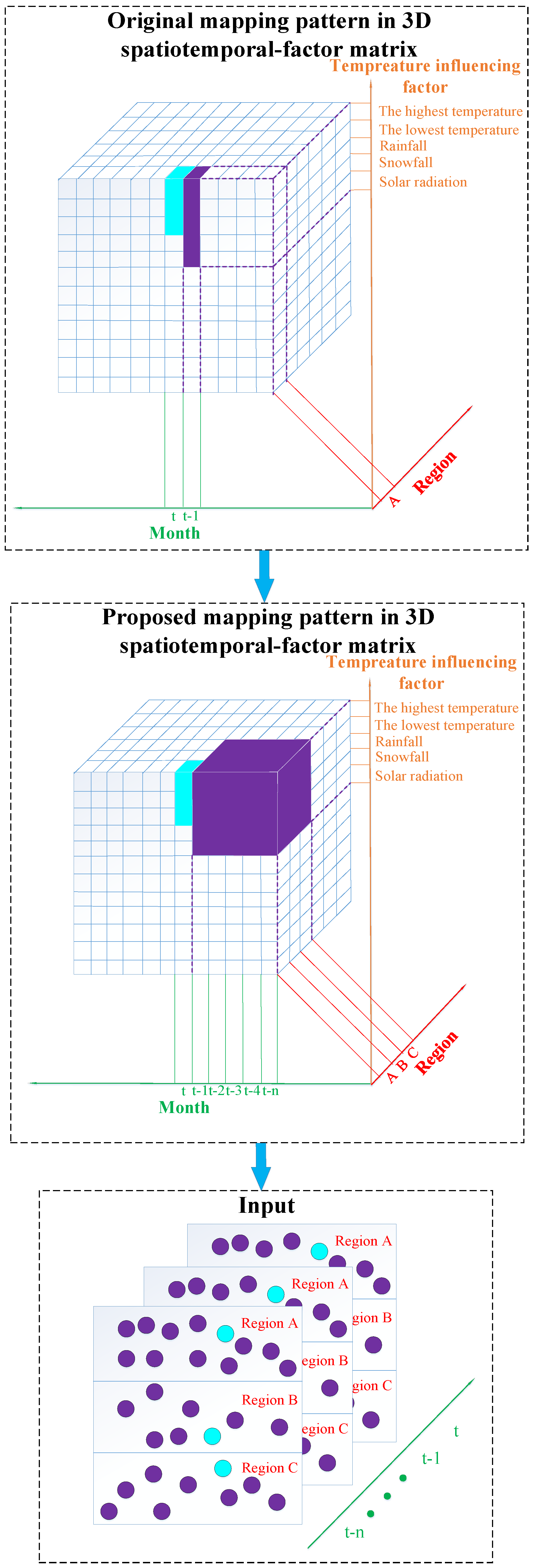
2.5. Three-Dimensional Input Conversion Technology for Data Dimensionality Upgrading in a Novel Spatiotemporal-Factor Matrix

Prior to the variables in each algorithm, it is crucial to optimize the number of informative features to enhance the prediction accuracy. As such, we have introduced a novel three-dimensional cubic framework, which enables more efficient feature selection. The cubic is composed of three axes: the x-axis represents the temporal dimension (i.e., month), the y-axis corresponds to the spatial dimension (i.e., latitude of different areas) and the z-axis refers to the climate impact factor. The cubic is rasterized based on a matrix form, where each grid corresponds to a specific matrix element at a specific coordinate in the matrix cubic.

Subsequently, select input variables from the matrix cubic. In traditional approaches for processing time-series data, input variables were mostly presented to the 3D spatiotemporal-factor matrix in a linear input form. For instance, the highest and lowest temperature of the previous month and the temperature-influencing factor determined by the principal component analysis method are taken as the input, while the highest temperature, the lowest temperature and rainfall of the next month are taken as the output. This mapping pattern reflects a linear-type input to linear-type output. The model established using this method predicts one month’s output with one month’s input. It extends the z-axis dimension of the 3D spatiotemporal-factor matrix. However, the other two axes are without expansion. The input presented in the 3D spatiotemporal-factor matrix takes the form of a line.

In this paper, the input-output mapping pattern was improved by expanding the x-axis and y-axis. Specifically, the highest temperature, the lowest temperature, rainfall, snowfall and solar radiation of regions A, B and C within a latitude difference of ±2° over the past $n$ months were selected as the input to predict the temperature and rainfall of region A in the $n+1$ month. This approach enables the prediction of one month’s output using $n$ months’ input along the x-axis and the prediction of one area’s output using three areas’ input along the y-axis, thus expanding all three axes. The mapping pattern of input and output can be described as body-type input to linear-type output. Figure 6 demonstrates the effectiveness of this innovation. The improved input-output mapping pattern offers two advantages: first, it significantly enhances the accuracy of prediction; and second, it increases the amount of data that are repeatedly called, similar to LSTM, allowing the system to determine the importance of the data. This feature prevents the prediction data from becoming unstable due to short-term climate mutation, which enhances the robustness of the corresponding system. The improved input-output mapping pattern was applied to all models in this study, resulting in the corresponding extension algorithms. The suffix “E” was added to the name of each novel algorithm to indicate that it has been extended.

2.6. Evolutionary Algorithm for Model Optimization

The intelligent algorithm proposed in this paper employs a neural network model, which inherently introduces randomness in the initial selection of weights and thresholds. Due to the significant impact of such initial values on the accuracy of network prediction, it becomes necessary to utilize an optimization algorithm to ensure that the initial weight and threshold values are as reasonable as possible. This process is referred to as “model optimization”. It is feasible to implement the PSO method because there are only a few interfaces for parameter adjustment in the LSTM neural network. In addition, the PSO algorithm has demonstrated the advantage of fast convergence, making it a suitable candidate for efficient climate data prediction in long time series. Therefore, in this study, the proposed model is optimized using the PSO algorithm.

PSO is a kind of evolutionary algorithm, akin to Simulate Anneal (SA) [35]. It starts with a random solution and iteratively searches for an optimal solution while evaluating its quality through fitness. Unlike the Genetic Algorithm (GA), which involves “crossover” and “mutation” operations, PSO directly seeks a global optimum by following the current optimal value. This algorithm simulates the foraging behavior of birds, where a group of birds randomly searches for food in an area with only one food source. The birds do not know the location of the food, but they can determine their distance from it. Moreover, they know the location of “bird A” that is closest to the food, which is the current global optimum. Consequently, each bird moves towards bird A, and in the process of approaching, each bird must locate the position closest to the food, which is the local optimal location of each bird.

Abstracted as point particles devoid of mass and volume, birds are extrapolated into n-dimensional space. The position of particle $i$ in n-dimensional space is represented as vector $X_i=(x_1,x_2,\cdots ,x_n)$, while its corresponding flight speed is represented as vector $V_i=(v_1,v_2,\cdots ,v_n)$. The fitness value of each particle is contingent on the objective function, and the particle is cognizant of both its optimal position (pbest) and its present position. This awareness can be seen as the particle’s individualistic flight experience.

In addition, each individual particle retains the knowledge of the best position (gbest) attained by all the particles in the entire population so far. Thus, while pbest denotes the current local optimal value, gbest represents the current global optimal value and can be deemed as the aggregate experience of the community. The particles’ subsequent actions are contingent upon their own experiences as well as the optimal experience of their peers.

Next, the optimal solution is derived via the iterative operation of random particles. During each iteration, particles recalibrate their velocity and position by tracking two “extremum” values (pbest, gbest). The algorithmic details are as follows:

Step 1: initialization.

To begin the Particle Swarm Optimization (PSO) process, the user must first determine the maximum number of iterations, the number of independent variables and the maximum speed of the particles. The initial speed and position of each particle within the speed range and the entire search space are then randomized. Additionally, set the particle swarm scale as $M$, and randomly initialize the flight speed of each particle.

Step 2: update of the global optimal solution

The fitness function is determined, and the individual extremum is defined as the optimal solution of each particle, which represents a local optimal solution. The current global optimal solution is derived by evaluating the optimal solutions obtained from all particles. Subsequently, the updating procedure is conducted by comparing the current global optimal solution with the historical global optimal solution.

Step 3: update of speed and position

The particles update their speed and position as follows:

$$v_{i+1}=\omega \cdot v_i+c_1\cdot rand()\cdot (pbes{t}_i-x_i)+c_2\cdot rand()\cdot (gbes{t}_i-x_i)$$

(2)

$$x_{i+1}=x_i+v_{i+1}$$

(3)

where $\omega$ is the inertia factor, the larger the value, the stronger the global optimization ability and the weaker the local optimization ability; $v_i$ is the particle speed at time $i$; $rand()$ is a random number between 0~1; $x_i$ is the position of the particle at time $i$; $c_1,c_2$ is the learning factor.

2.7. Proposed Climate Prediction System Named SS-OS-PSO-DBN-ELM-LSTME (SOPDEL)

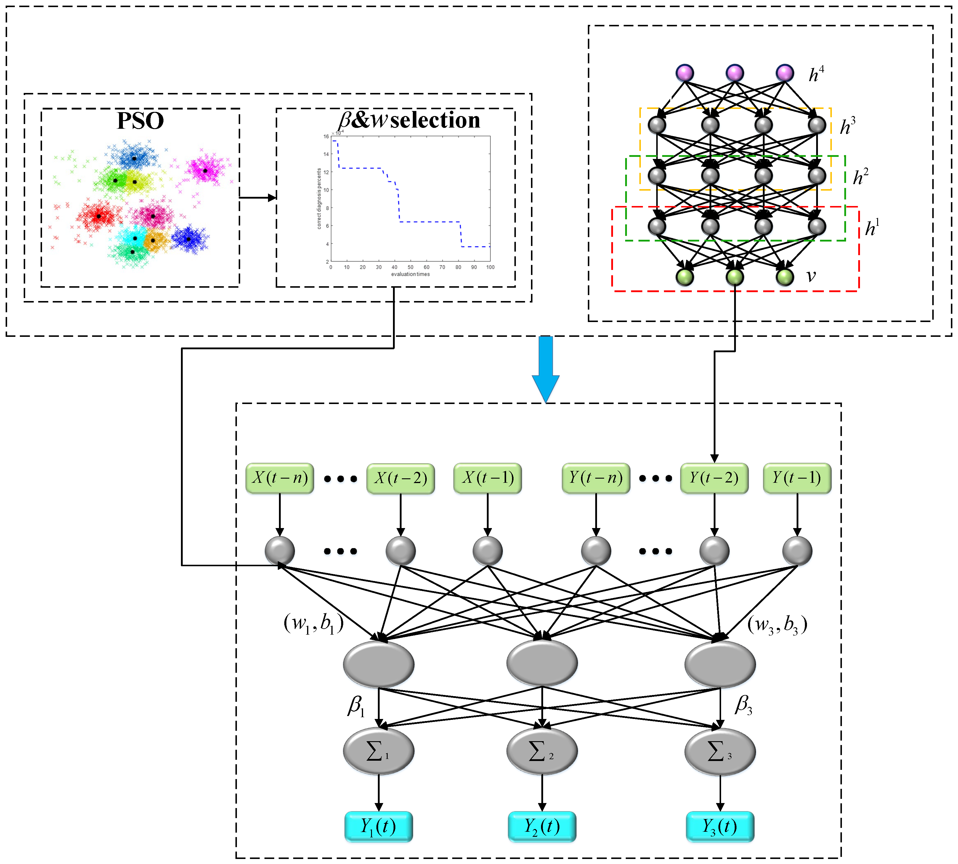
2.7.1. PSO-DBN-ELME Algorithm

In terms of network structure, an ELM is a type of Single-Hidden-Layer Forward Propagation Neural Network (SLFN) [36,37,38]. Unlike traditional neural networks that rely on gradient-based algorithms during the training phase, an ELM uses random input layer weights and biases. The output layer weights are calculated using generalized inverse matrix theory. Once the weights and biases of all network nodes are obtained, the ELM training is completed. An ELM is characterized by its ability to set the connection weight of the input layer and hidden layer randomly, as well as the threshold value of the hidden layer. Once set, there is no need to adjust them again, which greatly reduces computation compared to the BP neural network. Moreover, the connection weight does not need to be adjusted iteratively, it is determined at one time by solving equations. These features make the ELM highly computationally efficient with good generalization performance.

Suppose a given training set $P$ has $N$ arbitrary sample $(x_i,t_i)$, $x_i$ represents the $i$^th data sample; $t_i$ represents the $i$^th corresponding mark of the data sample. The training data set satisfies the equation $P=\left\{\left.(x_i,t_i)\right|x_i\in R^D,t_i\in R^m,i=1,2,\cdots ,N\right\}$.

For an ELM neural network, the input is the training sample set, the input layer is fully connected to the hidden layer. The output of the hidden layer is recorded as $H(x)$:

$$H(x)=\left[h_1(x),h_2(x),\cdots ,h_L(x)\right]$$

(4)

$h_i(x)$ is recorded as the output of the $i$th hidden layer node:

$$h_i(x)=g(w_i,b_i,x)=g(w_{i}x+b_i)$$

(5)

where $w_i,b_i$ is the hidden layer node parameter; $g(w_i,b_i,x)$ is the activation function, and the hidden layer parameter is initialized randomly. Then, the nonlinear mapping is used as the activation function to map the input data to a new feature space, and the Sigmoid activation function is selected in the circumstance.

Therefore, the output of the whole neural network can be expressed as follows:

$$f_L(x)={\displaystyle \sum _{i=1}^L{\beta }_i{h}_i(x)=H(x)\beta }$$

(6)

where ${\beta }_i$ is the weight of the $i$^th output.

Next, the objective function needs to be constructed to solve the output weight ${\beta }_i$, and the learning goal of the single-hidden-layer neural network is to minimize the output error. Therefore, the weight of the connection can be solved by minimizing the square error. The objective function is as follows:

$$\min {‖H\beta -T‖}^2,\beta \in R^{L\times m}$$

(7)

$$H={\left[h(x_1),h(x_2),\cdots ,h(x_N)\right]}^T=\left[\begin{array}{cccc}{h}_1(x_1)& h_2(x_1)& \cdots & h_L(x_1)\\ h_1(x_2)& h_2(x_2)& \cdots & h_L(x_2)\\ ⋮& ⋮& ⋮& ⋮\\ h_1(x_N)& h_2(x_N)& \cdots & h_L(x_N)\end{array}\right],T=\left[\begin{array}{c}{t}_1^T\\ t_2^T\\ ⋮\\ t_N^T\end{array}\right]$$

(8)

where $H$ is the output matrix of the hidden layer; $T$ is the target matrix of the training data.

The single objective programming model is solved and Equation (9) is obtained:

$$\beta =H^{+}T$$

(9)

where $H^{+}$ is the Moore Penrose generalized inverse matrix of $H$.

In this paper, characteristic data generated by a DBN were input into an ELM neural network for prediction. The specific algorithm is shown in Section 2.4.

PSO was employed to obtain values for initial thresholds and weights, i.e., $w,\beta$. Combined with the body-type input pattern in the new matrix, a PSO-DBN-ELME algorithm was constructed for climate prediction. The corresponding flow chart is shown in Figure 7.

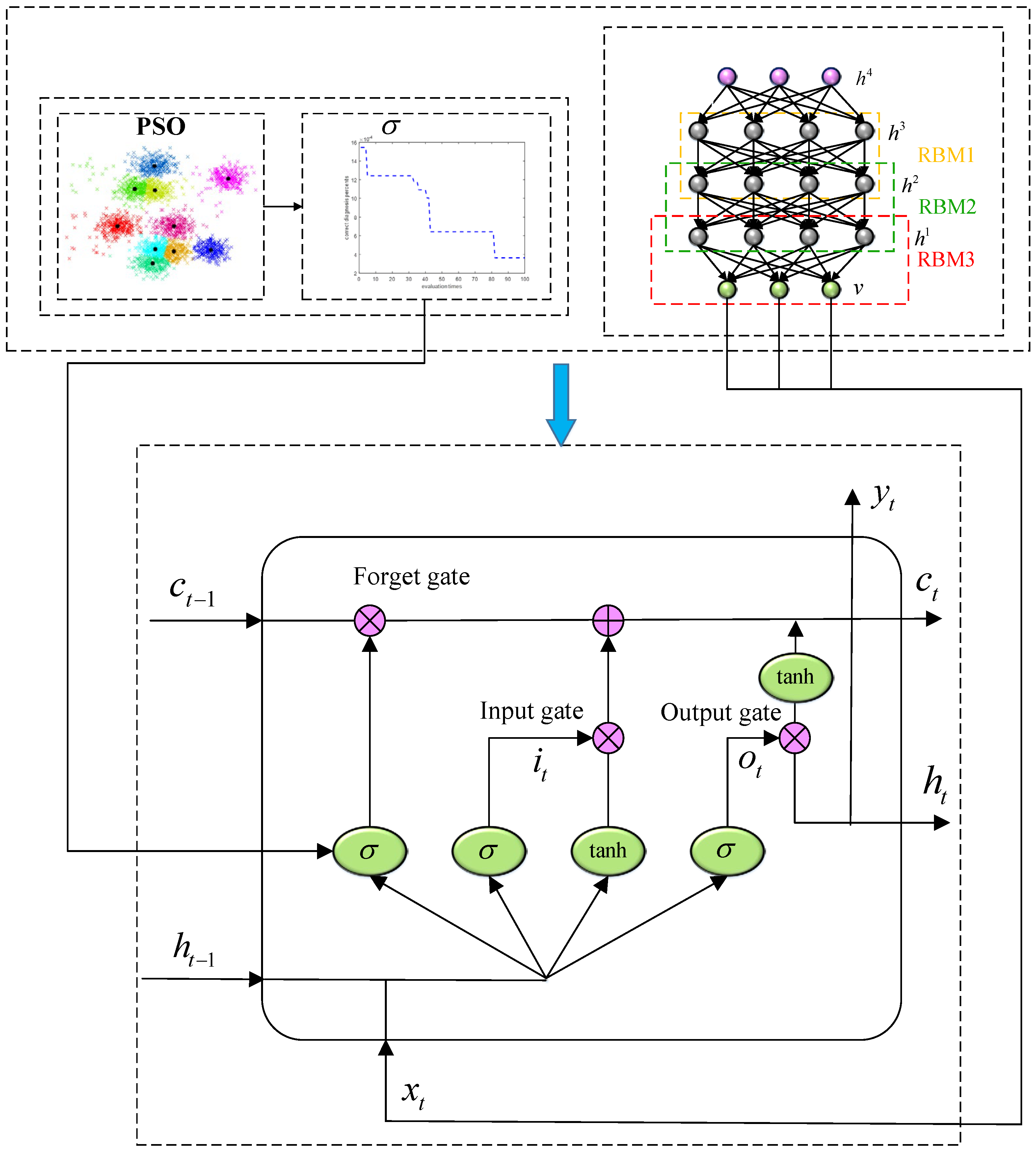
2.7.2. PSO-DBN-LSTME Algorithm

A Recurrent Neural Network (RNN) is a kind of neural network designed for processing sequential data. However, during the training phase, the gradient of a RNN may suffer from the issues of either vanishing or exploding. To mitigate this problem, LSTM has been developed as an evolved model of a RNN. LSTM can address the shortcomings of a RNN and exhibit superior performance in long-term training [39,40,41,42,43,44,45,46,47].

The architecture of Long Short-Term Memory (LSTM) differs from the traditional Recurrent Neural Network (RNN) as it comprises four network layers, as opposed to a single layer. The cell structure of LSTM is depicted in Figure 8. There are three gates to control the cell state, which are called the forget gate, input gate and output gate.

(1)

Forget gate: Determine which information in cell needs to be discarded. Output a vector by viewing the information of $h_{t-1}$ and $x_t$. The element’s value of 0~1 in the vector indicates how much information in cell state $c_{t-1}$ needs to be retained or discarded; 0 means no reservation, 1 means all reservation.

(2)

Input gate: Determine which information in the cell needs to be updated. Firstly, $h_{t-1}$ and $x_t$ are used to determine the information to be updated, and then new candidate cell information ${\tilde{c}}_t$ is obtained through a $\tanh$ layer, which may be updated into the cell information. For the update of the old cell information $c_{t-1}$ to the new $c_t$, the rule is to forget part of the old cell information by the selection of the forget gate, and $c_t$ is obtained by inputting part of the candidate cell information ${\tilde{c}}_t$ by gate selection.

(3)

Output gate: Determine which information in the cell needs to be output. The output is activated by the $\tanh$ function, and it needs to enter the Sigmoid layer to get the judging condition of the cell’s output state characteristics. The final output of the LSTM cell is obtained by multiplying the judging condition of the input and output gate.

In this paper, characteristic data generated by DBN were input into a LSTM neural network for prediction. The specific algorithm is shown in Section 2.4.

PSO was also employed in the same way as it in the PSO-DBN-ELME algorithm. Combined with the body-type input pattern, the PSO-DBN-LSTME algorithm was constructed for climate prediction. The corresponding flow chart is shown in Figure 8.

2.7.3. SOPDEL Algorithm

The proposed SOPDEL algorithm has been suggested as a viable system for climate prediction. This algorithm is a combination of the PSO-DBN-ELME and PSO-DBN-LSTME algorithms, which are utilized in different time series. To achieve this, the PD-RS-PE technology is utilized for data decomposition, and output data for stationary and oscillatory series are separately predicted using PSO-DBN-LSTME and PSO-DBN-ELME. Furthermore, the time coordinates of different data series are used to fuse the two prediction series to form the final climate prediction data.

2.8. Performance Evaluation Indices

In this paper, four indicators, including the root mean square error ($RMSE$), mean absolute error ($MAE$), mean absolute percentage error ($MAPE$) and correlation coefficient ($R^2$), were employed as evaluation criteria to quantitatively assess the forecasting performance of each proposed model. These indicators can be formulated as follows:

$$RMSE=\sqrt{\frac{1}{n}{\displaystyle \sum _{i=1}^n{(x_i-{\widehat{x}}_i)}^2}}$$

(10)

$$MAE=\frac{1}{n}{\displaystyle \sum _{i=1}^n\left|x_i-{\widehat{x}}_i\right|}$$

(11)

$$MAPE=\frac{1}{n}{\displaystyle \sum _{i=1}^n\left|\frac{x_i-{\widehat{x}}_i}{x_i}\right|}\times 100\%$$

(12)

$$R^2=\frac{({\displaystyle {\sum }_{i=1}^n{\widehat{x}}_i{x}_i-{\displaystyle {\sum }_{i=1}^n{\widehat{x}}_i}{\displaystyle {\sum }_{i=1}^n{x}_i/n{)}^2}}}{({\displaystyle {\sum }_{i=1}^n{\widehat{x}}_i{}^2-{({\displaystyle {\sum }_{i=1}^n{\widehat{x}}_i})}^2/n)}({\displaystyle {\sum }_{i=1}^n{\widehat{x}}_i{}^2-{({\displaystyle {\sum }_{i=1}^n{x}_i})}^2/n)}}$$

(13)

3. Nine Climate Forecasting Models for Comparison and Verification

In order to verify accuracy and stability of the proposed model, comparative models are formulated.

Firstly, we use LSTM as the basic model, then each improvement occurred in this paper is utilized one by one, which is abbreviated as M1~M5.

Model 1 (M1): an ordinary LSTM neural network, using no optimization and data processing;

Model 2 (M2): on the basis of model 1, the three-dimensional input conversion technology was applied to improve the robustness of the LSTM neural network, forming the LSTME model;

Model 3 (M3): on the basis of model 2, a DBN was used to extract features from the original data, the feature data was used as the input of the LSTM, forming a DBN-LSTME model;

Model 4 (M4): on the basis of model 3, PSO was used to optimize the weights and thresholds between and within each layer in the LSTM, forming a PSO-DBN-LSTME model;

Model 5 (M5): an ELM neural network was introduced, the weight and threshold between and within each layer were optimized by PSO. The original data were extracted by a DBN, and the feature data were used for the input of the LSTM. A PSO-DBN-LSTME model was formed by combining the new mapping and extracting mode of the input, the prediction results were averaged with the ones generated by model 4, a PSO-DBN-ELM-LSTME model was formed by integrating the two methods on each prediction result;

Model 6 (M6): model 6 is proposed in this research paper and incorporates the memory and forget mechanism of a LSTM neural network to produce smoother prediction results, while also utilizing the strong fitting ability of an ELM neural network for extreme data. To further enhance the performance of the model, the PD-RS-PE technology is introduced to divide the input data into a stationary and oscillatory series, with LSTM used for the former and an ELM for the latter. The weights and thresholds of the two networks are optimized using PSO. The original data are preprocessed using a DBN. Combined with new mapping and extracting mode of input, a SOPDEL model was finally formed.

In addition, we also introduced three classical traditional models for state-of-the-art climate prediction. It aims to compare the prediction performance of M6 with that of previous models.

Model 7 (M7): an Autoregressive Integrated Moving Average (ARIMA) model, which has become one of the most widely-used climate prediction methods from the perspective of time series characteristics in climate itself.

Model 8 (M8): an Echo State Network (ESN) model, which is a new recursive neural network, has been gradually applied to climate prediction due to its simple structure and fast convergence.

Model 9 (M9): a Support Vector Machine (SVM) model, which overcomes the problems of dimensionality disaster and nonlinear separability, and has achieved certain prediction results in climate data with complex nonlinear characteristics.

4. Results and Discussion

4.1. Comparative Analysis for Fitting Performance in Training Datasets between M1–M9 Models

In order to prove the best prediction performance, these six models in chapter 3 were comprehensively analyzed and compared in this study. In order to determine which types of input data are needed to predict the output data, correlation analysis was carried out for the highest temperature (HT), the lowest temperature (LT), rainfall (RF), snowfall (SF) and solar radiation (SR) of the three studied areas. The corresponding results are shown in Figure 9. The correlation coefficient is between −1 and 1. The greater the positive (negative) value is, the stronger the correlation (anticorrelation) gets. We made a rule that if $x$ is selected as the input data to predict the output data $y$, the absolute value of the correlation coefficient between $x$ and $y$ is greater than 0.4. According to it, the input data of predicting HT and LT in the last month are HT, LT, RF, SF and SR in the previous month, the independent variables of RF in the last month are HT, LT and RF in the previous month, the independent variables of SF are HT, LT and SF in the previous month and the independent variables of SR in the last month are HT, LT and SR in the previous month.

All data were divided into a training set and testing set. According to the combination of independent variables and dependent variables, the five dependent variables were predicted. $R^2$, $RMSE$, $MAE$ and $MAPE$ were selected as indexes to evaluate the fitting accuracy of each model for the training dataset, and the effect is shown in

Table 1. Performance evaluation indices for M1–M6 models in training dataset.

Climate Data	Model	$R^2$	$RMSE$	$MAE$	$MAPE$
The highest temperature	M6	0.9944	0.4463	0.3243	0.0007
	M5	0.9910	0.5599	0.3438	0.0006
	M4	0.9742	0.9374	0.7041	0.0005
	M3	0.9718	0.9799	0.7647	0.0005
	M2	0.9693	1.0472	0.6684	0.0008
	M1	0.9614	1.1529	0.7971	0.0009
The lowest temperature	M6	0.9900	0.4760	0.3599	0.0002
	M5	0.9791	0.6888	0.4303	0.0006
	M4	0.9673	0.8625	0.6158	0.0019
	M3	0.9584	0.9710	0.7353	0.0017
	M2	0.9444	1.1374	0.7276	0.0026
	M1	0.9397	1.1818	0.7875	0.0027
Rainfall	M6	0.9669	11.3331	8.2658	0.0001
	M5	0.9602	12.4948	7.7168	0.0005
	M4	0.7880	28.4910	19.9793	0.0081
	M3	0.7239	32.5228	24.3261	0.0100
	M2	0.5611	41.2722	28.5648	0.0208
	M1	0.5259	42.8850	30.6940	0.0221

. In this table, for the optimal values of each index, it can be seen that 83% of optimal values is concentrated in the SOPDEL (M6) model, displayed in bold font. The phenomenon shows that compared with the other five models, the M6 model has a higher fitting performance for training data. Among the best evaluation indexes of the M6 model, $R^2$ increased by 83.9% at most compared with the lowest value, $RMSE$ decreased by 73.6% at most compared with the highest value, $MAE$ decreased by 73.1% at most compared with the highest value and $MAPE$ decreased by 99.5% at most compared with the highest value, which reflected that improvement of the fitting effect was very obvious. Figure 10, Figure 11 and Figure 12 show the fitting ability of each model. In general, the M6 model outperforms the other hybrid models with the highest coefficient of correlation coefficient ($R^2$) value, and displays a better fitting ability of the highest temperature, the lowest temperature and rainfall, which can reflect climate extremes.

The comparison of fitting performance of M1 and M2, M2 and M3, M3 and M4 and M5 and M6, respectively, shows that three-dimensional input conversion technology, DBN feature extraction, PSO optimization and PD-RS-PE technology have all played an effective role in improving the accuracy of the model, which proves that all optimization and data processing methods proposed in this paper can improve the fitting accuracy of the climate prediction model.

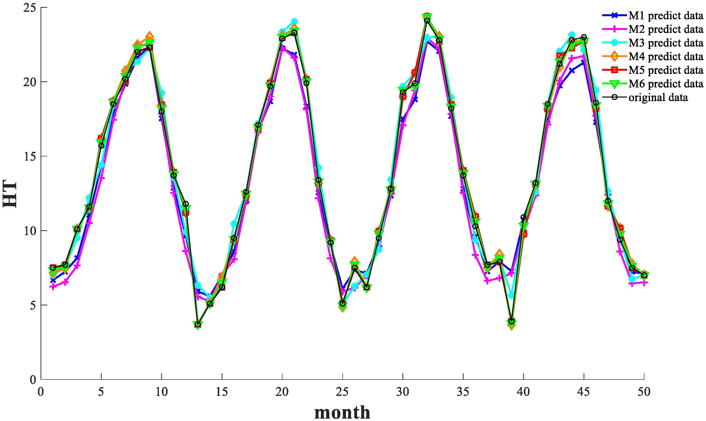
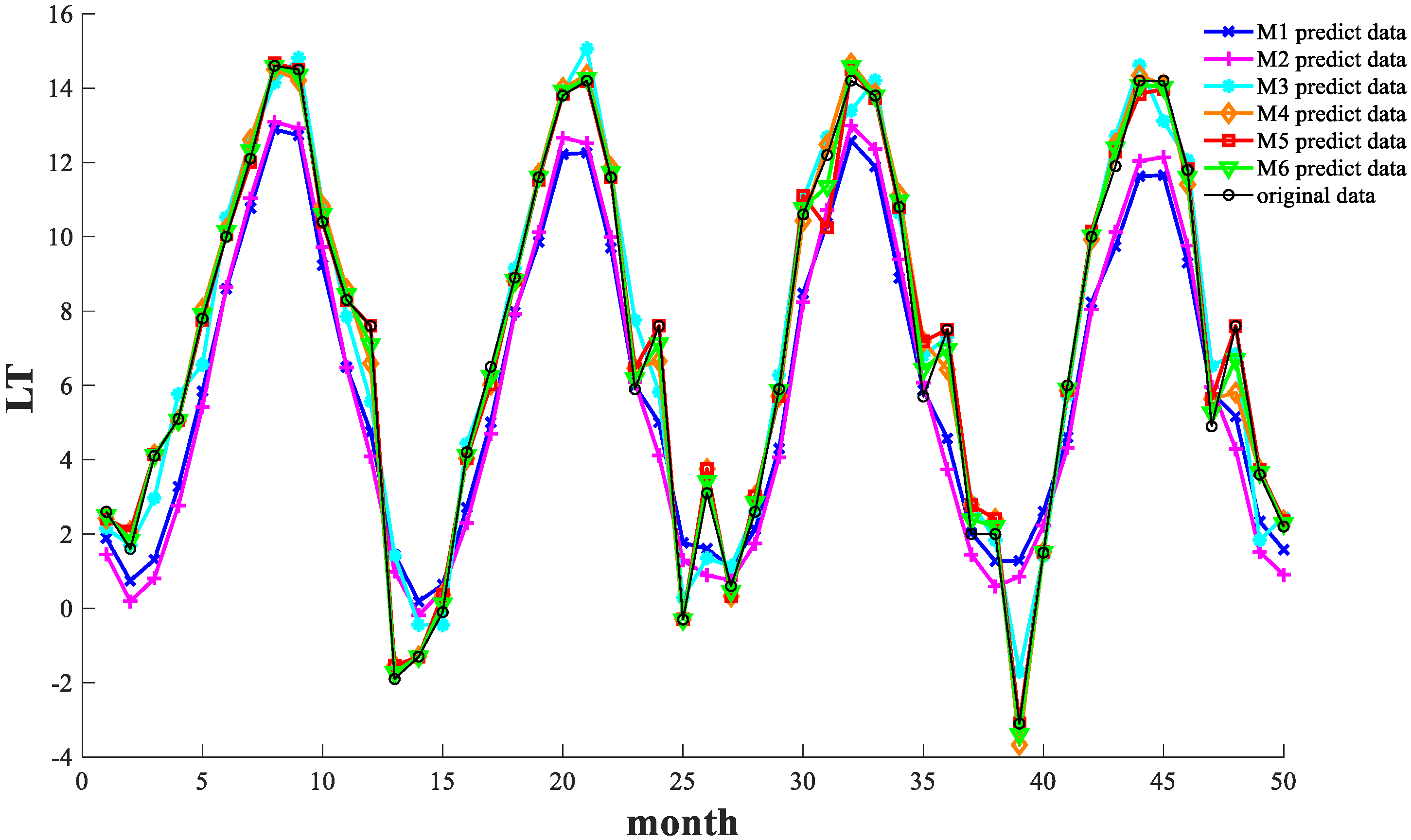
4.2. Comparative Analysis for Predicting Performance in Testing Datasets between M1–M6 Models

After fitting the training datasets, performance of prediction of each model should be compared in case of an overfitting phenomenon of some training models. $R^2$, $RMSE$, $MAE$ and $MAPE$ were selected as indexes to evaluate the prediction accuracy of each model for the testing set, and the effect is shown in

Table 2. Performance evaluation indices for the six proposed models in testing dataset.

Climate Data	Proposed Model	$R^2$	$RMSE$	$MAE$	$MAPE$
The highest temperature	M6	0.9990	0.1981	0.1632	0.0052
	M5	0.9972	0.3312	0.2206	0.0032
	M4	0.9964	0.3836	0.3085	0.0126
	M3	0.9835	0.7985	0.5936	0.0092
	M2	0.9805	1.1110	0.8832	0.0932
	M1	0.9710	1.2862	1.0848	0.1051
The lowest temperature	M6	0.9964	0.2986	0.2141	0.0004
	M5	0.9924	0.4476	0.2515	0.0012
	M4	0.9890	0.5283	0.3814	0.0082
	M3	0.9633	0.9583	0.7018	0.0062
	M2	0.9314	1.8562	1.6509	0.3455
	M1	0.9147	1.9314	1.7136	0.3332
Rainfall	M6	0.9934	5.9639	4.8788	0.0206
	M5	0.9908	7.0205	3.6939	0.0327
	M4	0.9793	10.7810	8.5691	0.0484
	M3	0.8828	25.3663	19.0880	0.1493
	M2	0.7283	45.3143	35.5998	0.4868
	M1	0.6602	43.9278	33.6869	0.3867

. In this table, for the optimal value of each index, it is also displayed in bold font. It can be seen that 83% of the optimal value is concentrated on the SOPDEL (M6) model. Among the best evaluation indexes of the M6 model, $R^2$ increased by 50.5% at most compared with the lowest value, $RMSE$ decreased by 86.4% at most compared with the highest value, $MAE$ decreased by 87.5% at most compared with the highest value and $MAPE$ decreased by 99.9% at most compared with the highest value, reflecting that the improvement of the predicting effect was very obvious.

As is mentioned above in Section 4.1, all optimization and data processing methods proposed in this paper can improve the predicting accuracy of the climate prediction model.

Figure 13, Figure 14 and Figure 15 show the intuitive predicting ability of each model in the form of a trend chart.

4.3. Comparative Analysis for Fitting Performance in Training Datasets between M6–M9 Models

Next, a comparative experiment between the proposed model and the traditional classical climate prediction model is carried out. The results for the training data are shown in

Table 3. Performance evaluation indices for M6–M9 models in training dataset.

Climate Data	Model	$R^2$	$RMSE$	$MAE$	$MAPE$
The highest temperature	M6	0.9944	0.4463	0.3243	0.0007
	M7	0.9817	0.9079	0.7281	0.0032
	M8	0.9895	1.5036	1.1899	0.0005
	M9	0.9889	1.4249	1.1040	0.0003
The lowest temperature	M6	0.9900	0.4760	0.3599	0.0002
	M7	0.9733	0.9271	0.7168	0.0063
	M8	0.9090	1.4749	1.1457	0.0021
	M9	0.9251	1.3080	0.9647	0.0038
Rainfall	M6	0.9669	11.3331	8.2658	0.0001
	M7	0.9998	1.0390	0.7868	0.0004
	M8	0.3783	51.2115	38.7237	0.0253
	M9	0.4600	46.8355	34.4975	0.0402

. For the optimal values of each index, it can be seen that 67% of the optimal values is concentrated in the SOPDEL (M6) model, displayed in bold and red font. The phenomenon shows that, compared with the other three models, the M6 model has a higher fitting performance for the training data. Among the best evaluation indexes of the M6 model, $R^2$ increased by 8.9% at most compared with the lowest value, $RMSE$ decreased by 70.3% at most compared with the highest value, $MAE$ decreased by 72.7% at most compared with the highest value and $MAPE$ decreased by 99.8% at most compared with the highest value, which reflected that the improvement of the fitting effect was very obvious. Figure 16, Figure 17 and Figure 18 show the intuitive fitting ability of each model.

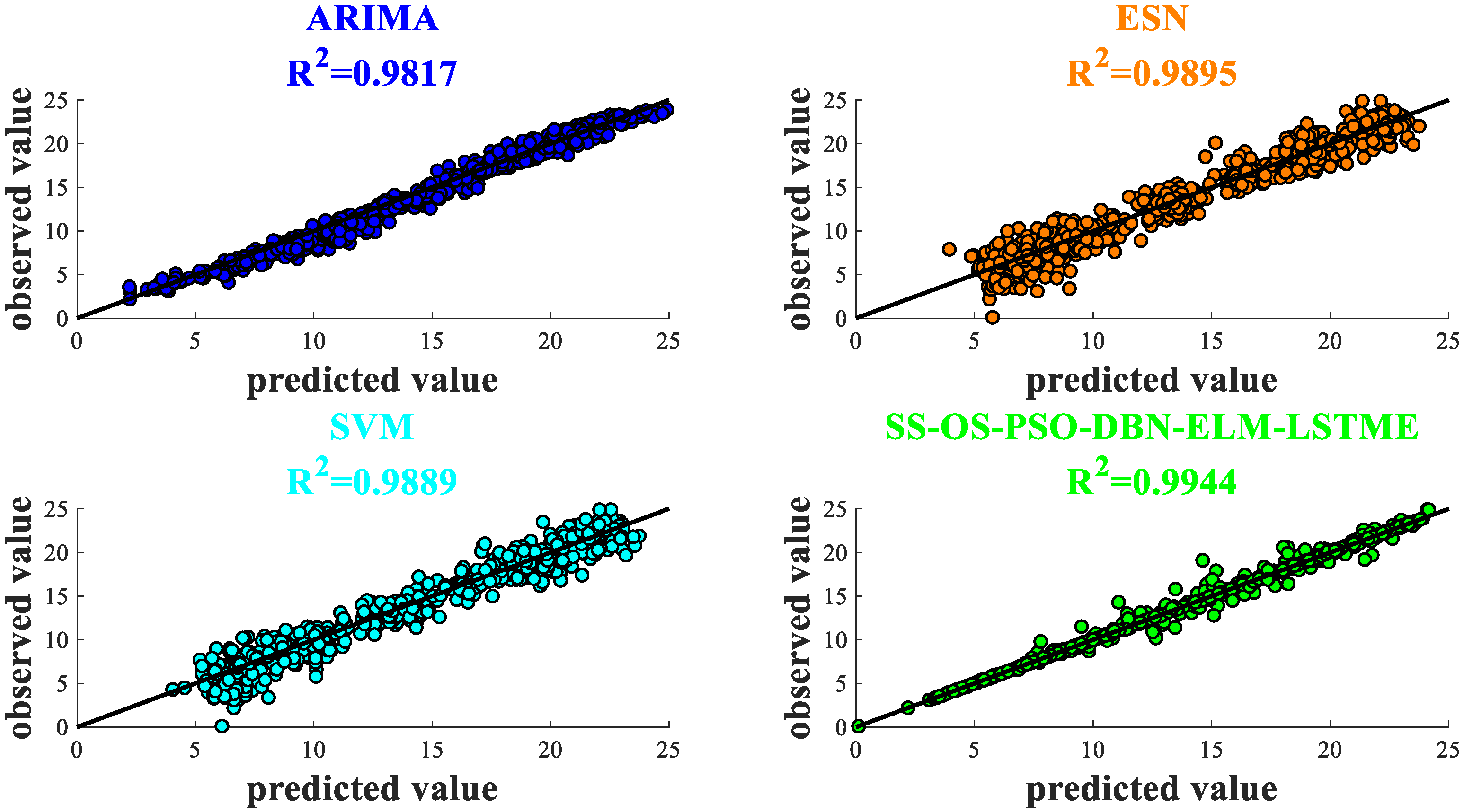
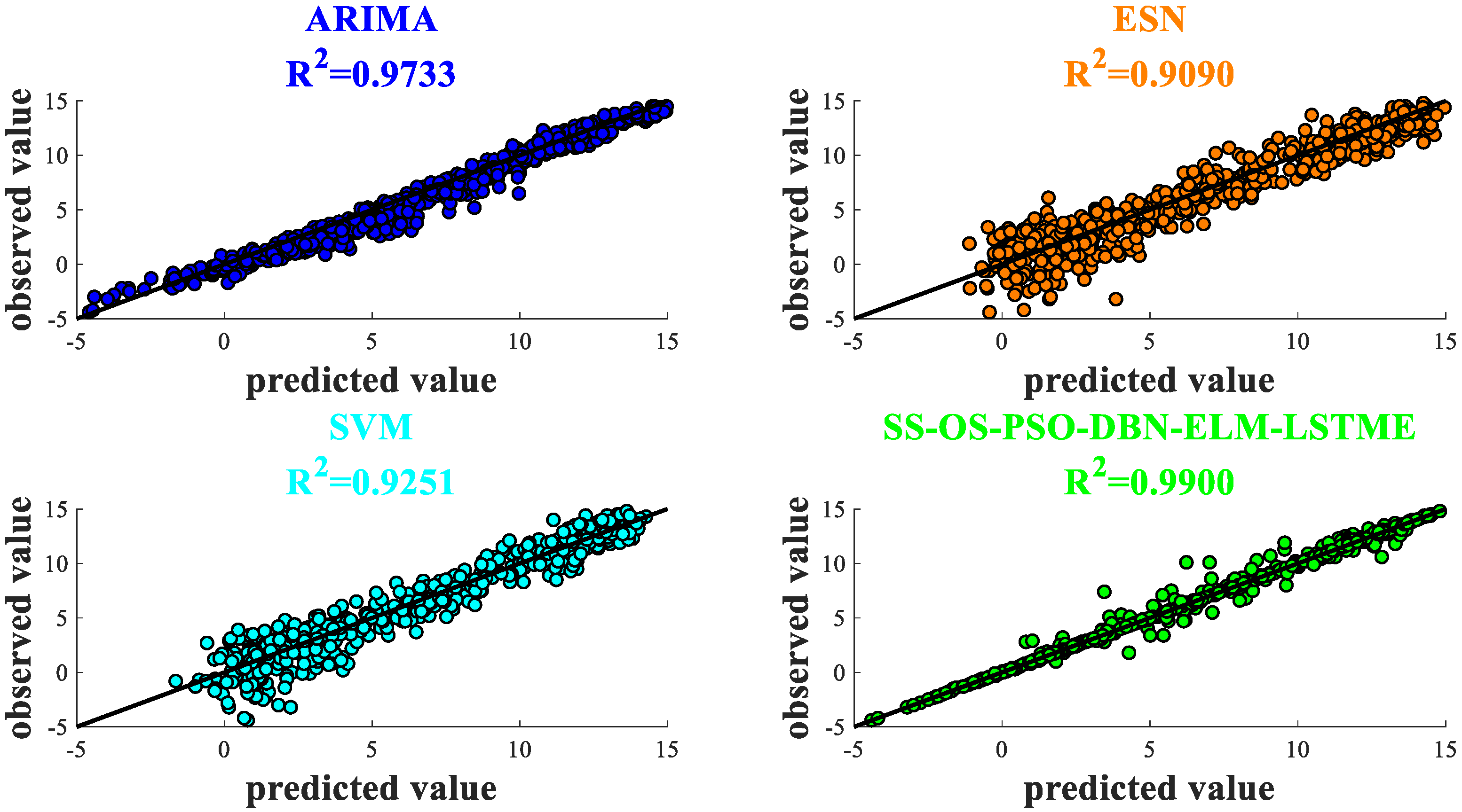
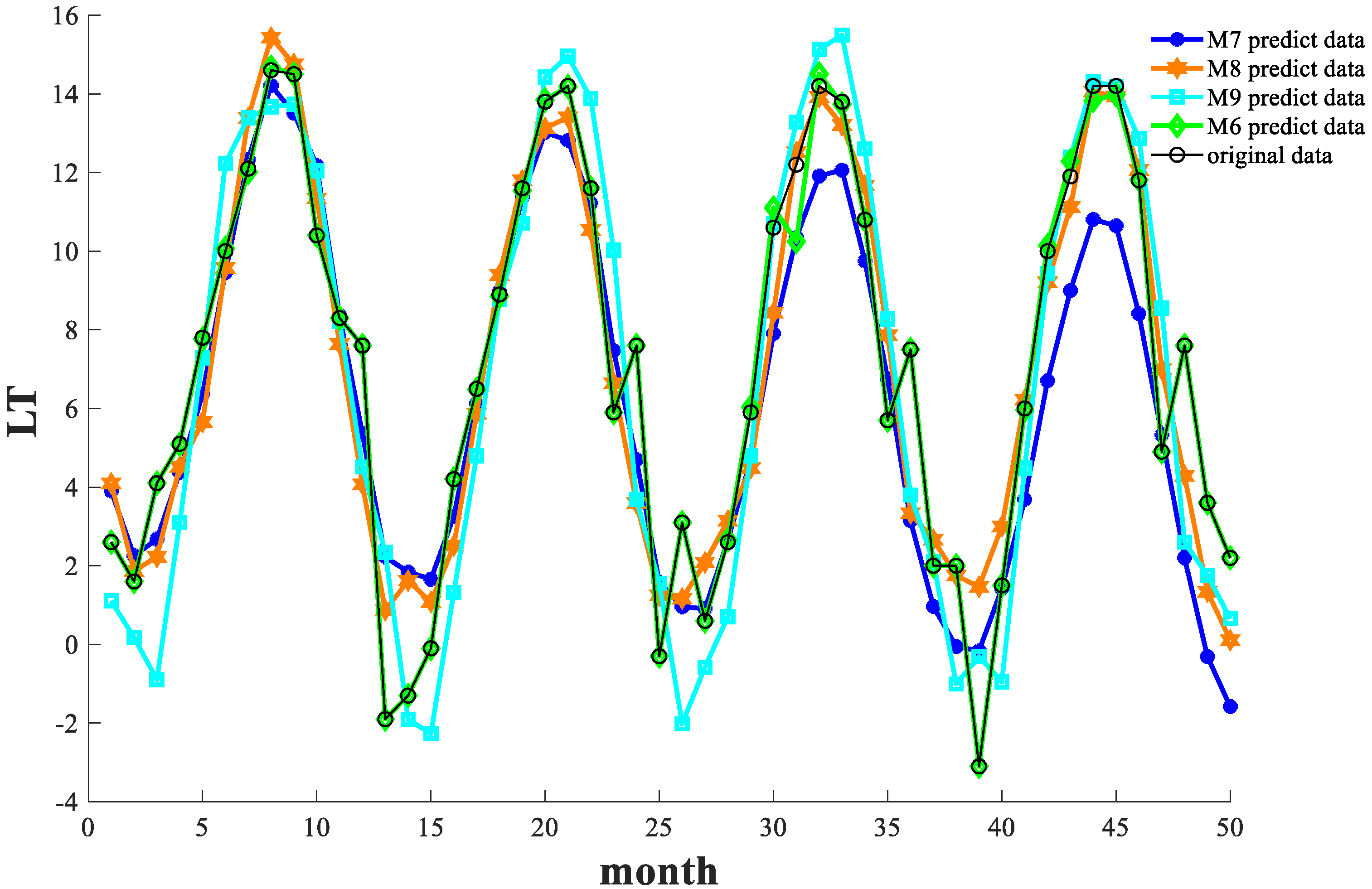
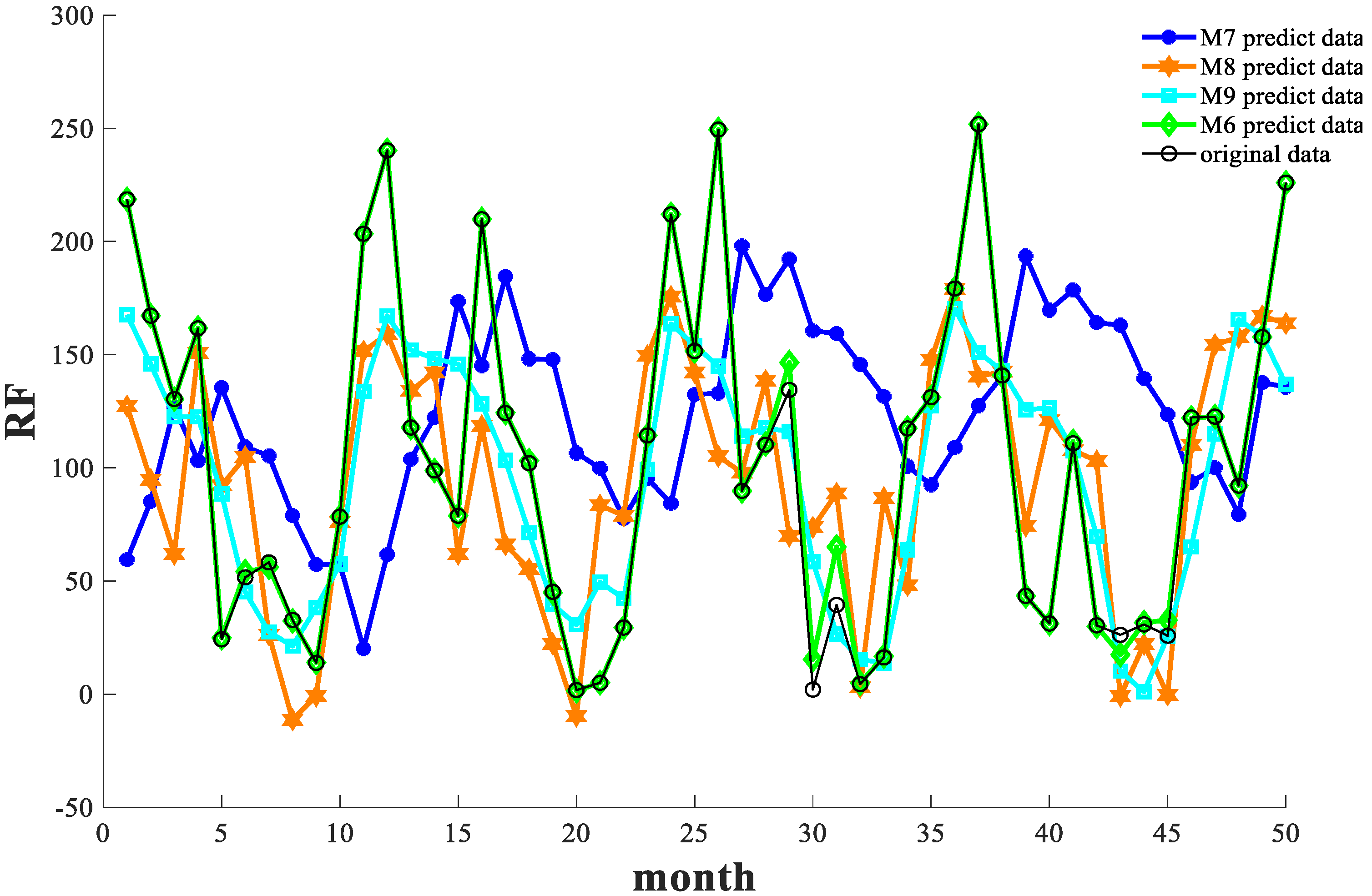
4.4. Comparative Analysis for Predicting Performance in Testing Datasets between M6–M9 Models

The results for testing data are shown in

Table 4. Performance evaluation indices for M6–M9 models in testing dataset.

Climate Data	Model	$R^2$	$RMSE$	$MAE$	$MAPE$
The highest temperature	M6	0.9990	0.1981	0.1632	0.0052
	M7	0.8455	5.9297	5.4070	0.6155
	M8	0.9893	1.5866	1.2181	0.0972
	M9	0.9900	2.1328	1.8084	0.0601
The lowest temperature	M6	0.9964	0.2986	0.2141	0.0004
	M7	0.8383	2.2091	1.7702	0.2982
	M8	0.8762	1.7638	1.3624	0.1071
	M9	0.8549	2.2919	1.8396	0.0267
Rainfall	M6	0.9934	5.9639	4.8788	0.0206
	M7	0.0541	93.2919	79.0570	0.4900
	M8	0.4590	54.3568	43.6699	0.4365
	M9	0.6106	46.1647	35.2501	0.3776

, for optimal values of each index, it can be seen that 100% of optimal values is concentrated in the SOPDEL (M6) model, displayed in bold font. The phenomenon shows that, compared with the other three models, the M6 model has a higher predicting performance for testing data. It is worth noting that M7 has an extreme distortion in predicting the rainfall test set, which is mainly due to an over-fitting phenomenon caused by the training set. Except that, among the best evaluation indexes of the M6 model, $R^2$ increased by 116.4% at most compared with the lowest value, $RMSE$ decreased by 96.7% at most compared with the highest value, $MAE$ decreased by 97% at most compared with the highest value and $MAPE$ decreased by 99.9% at most compared with the highest value, which reflected that the improvement of the predicting effect was very obvious. Figure 19, Figure 20 and Figure 21 show the intuitive fitting ability of each model.

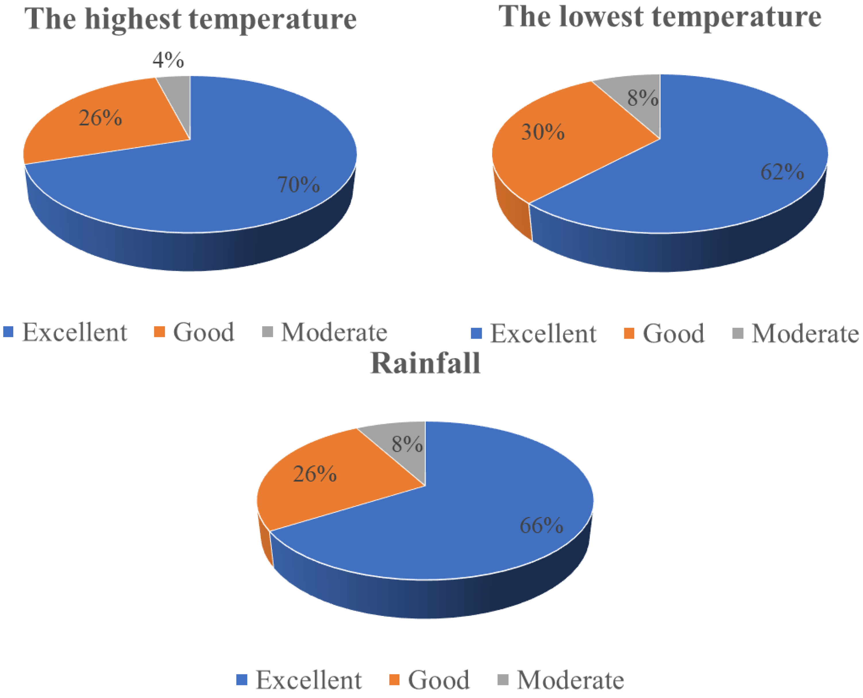
4.5. Predicting Performance for the Proposed Model

According to comparison tests for each model, we can draw the conclusion that the proposed SOPDEL model is the best model among all nine models. Therefore, further tests should be carried out to evaluate the performance of the M6 model. In this study, the monthly climate data of the target area from December 2015 to January 2020 were predicted using M6, and the predicted value was compared with the real one. Based on the error between the predicted value and the real value, the corresponding evaluation system was set up as follows:

Evaluation system of maximum and minimum temperature:

(1)

When the error is within ±0.2 °C, it is judged that the prediction quality of the month is very prominent, which is expressed as “Excellent”;

(2)

When the error is between ±0.2 °C and 0.5 °C, it is judged that the prediction quality of the month is good, which is expressed as “Good”;

(3)

When the error is within ±0.5~1 °C, it is judged that the prediction quality of the month is medium, which is expressed as “Moderate”;

(4)

When the error is beyond ±1 °C, it is judged that the prediction quality of the month is poor, which is expressed as “Bad”.

(5)

Evaluation system of rainfall:

(6)

When the error is within ±5mm, it is judged that the prediction quality of the month is very prominent, which is expressed as “Excellent”;

(7)

When the error is within ±5~10 mm, it is judged that the prediction quality of the month is good, which is expressed by “Good”;

(8)

When the error is within ±10~20 mm, it is judged that the prediction quality of the month is medium, which is expressed by “Moderate”;

(9)

When the error is beyond ±20 mm, it is judged that the prediction quality of the month is poor, which is expressed as “Bad”.

According to the evaluation system above, we can acquire the effect of the prediction on each month’s climate data.

Table 5. Predicting performance for SOPDEL model under the evaluation system made in this study.

Date	The Highest Temperature (Unit: °C)			The Lowest Temperature (Unit: °C)			Rainfall (Unit: mm)
	Actual	Forecast	Quality	Actual	Forecast	Quality	Actual	Forecast	Quality
December 2015	7.5	7.3398	Excellent	2.6	2.5070	Excellent	218.6	208.2459	Good
January 2016	7.7	7.5826	Excellent	1.6	1.8390	Good	167.2	159.2228	Good
February 2016	10.1	10.1042	Excellent	4.1	4.1217	Excellent	130.4	137.5251	Good
March 2016	11.6	11.5474	Excellent	5.1	5.0720	Excellent	161.6	160.6963	Excellent
April 2016	15.7	15.9185	Good	7.8	7.9100	Excellent	24.2	16.4077	Good
May 2016	18.5	18.6536	Excellent	10	10.1467	Excellent	51.6	51.5732	Excellent
June 2016	20.2	20.3909	Excellent	12.1	12.3117	Good	58.2	47.6714	Moderate
July 2016	22	22.2694	Good	14.6	14.5930	Excellent	32.8	36.4994	Excellent
August 2016	22	22.6675	Moderate	14.5	14.3521	Excellent	13.8	13.3474	Excellent
September 2016	18	18.2240	Good	10.4	10.6100	Good	78.4	66.4883	Good
October 2016	13.7	13.8064	Excellent	8.3	8.4452	Excellent	203.4	198.4994	Excellent
November 2016	11.8	11.5107	Good	7.6	7.0967	Moderate	240.2	241.4955	Excellent
December 2016	3.7	3.7118	Excellent	−1.9	−1.7218	Excellent	117.8	112.8448	Excellent
January 2017	5.1	5.1253	Excellent	−1.3	1.2987	Excellent	98.8	99.7717	Excellent
February 2017	6.2	6.5295	Good	−0.1	0.1312	Excellent	78.8	75.8139	Excellent
March 2017	9.5	9.4452	Excellent	4.2	4.1198	Excellent	209.8	207.2923	Excellent
April 2017	12.6	12.4872	Excellent	6.5	6.2520	Good	124.2	122.0196	Excellent
May 2017	17.1	16.9661	Excellent	8.9	8.8326	Excellent	102	96.3386	Good
June 2017	19.7	19.7449	Excellent	11.6	11.6155	Excellent	45.2	41.6002	Excellent
July 2017	22.9	23.0222	Excellent	13.8	13.9241	Excellent	1.8	5.1026	Excellent
August 2017	23.3	23.4255	Excellent	14.2	14.2678	Excellent	5	7.3658	Excellent
September 2017	19.9	20.0255	Excellent	11.6	11.7353	Excellent	29.4	29.8482	Excellent
October 2017	13.4	13.2980	Excellent	5.9	6.1782	Good	114.3	128.4054	Moderate
November 2017	9.2	9.2724	Excellent	7.6	7.1276	Good	212	214.0281	Excellent
December 2017	5.1	4.9846	Excellent	−0.3	−0.2994	Excellent	151.6	149.0540	Excellent
January 2018	7.5	7.7038	Good	3.1	3.4227	Good	249.4	247.1281	Excellent
February 2018	6.2	6.1890	Excellent	0.6	0.4597	Excellent	89.8	98.0948	Good
March 2018	9.5	9.7942	Good	2.6	2.8414	Good	110.2	106.2041	Excellent
April 2018	12.8	12.7656	Excellent	5.9	5.8745	Excellent	134.4	139.7440	Good
May 2018	19.3	19.4378	Excellent	10.6	10.7660	Excellent	2	9.8711	Good
June 2018	19.9	19.7199	Excellent	12.2	11.3656	Good	39.4	52.8009	Moderate
July 2018	24.1	24.3585	Good	14.2	14.5827	Good	4.4	6.9913	Excellent
August 2018	22.8	22.8814	Excellent	13.8	13.7947	Excellent	16.2	12.2030	Excellent
September 2018	18.2	18.3292	Excellent	10.8	10.9668	Excellent	117.4	110.7052	Good
October 2018	13.7	13.8661	Excellent	5.7	6.4413	Moderate	131.2	119.9685	Moderate
November 2018	10.3	10.6193	Good	7.5	6.9648	Moderate	179.2	180.5537	Excellent
December 2018	7.7	7.6093	Excellent	2	2.3930	Good	251.8	247.2106	Excellent
January 2019	7.9	8.1561	Good	2	2.2026	Good	140.8	135.3906	Excellent
February 2019	3.9	3.7840	Excellent	−3.1	−3.3859	Good	43.4	41.1272	Excellent
March 2019	10.9	10.3358	Moderate	1.5	1.5063	Excellent	31.2	35.4759	Excellent
April 2019	13.2	13.1458	Excellent	6	5.9137	Excellent	110.8	103.8416	Good
May 2019	18.5	18.3757	Excellent	10	10.0341	Excellent	30.4	38.5369	Good
June 2019	21.2	21.3732	Excellent	11.9	12.3973	Good	26.2	18.7868	Good
July 2019	22.8	22.4856	Good	14.2	14.0893	Excellent	30.8	34.0751	Excellent
August 2019	23	22.7455	Good	14.2	14.0337	Excellent	25.8	30.1011	Excellent
September 2019	18.6	18.4169	Excellent	11.8	11.6109	Excellent	122.2	124.5298	Excellent
October 2019	12	11.8299	Excellent	4.9	5.2675	Good	122.6	118.3732	Excellent
November 2019	9.4	9.7790	Good	7.6	6.7031	Moderate	92.1	96.2326	Excellent
December 2019	7.5	7.6247	Excellent	3.6	3.6619	Excellent	157.8	156.9835	Excellent
January 2020	7	7.0094	Excellent	2.2	2.2843	Excellent	226	230.1365	Excellent

shows the detailed real value, predicted value and quality of each month, and Figure 22 shows the proportion of each quality in predicting climate data. It can be seen that for three kinds of climate data, the total proportion with the prediction quality of “Excellent” and “Good” has exceeded 90%, and no data with “bad” have appeared, indicating that the SOPDEL model is very stable and convincing, meeting the high requirements of short-term and long-term climate prediction.

5. Conclusions

Environmental protection has been a hot topic in the academic field and an accurate and stable climate forecast of our study can contribute well to this target. This study has proposed a novel hybrid spatiotemporal system as a promising alternative tool for long-term climate forecasting in practice. The proposed model, named SOPDEL, which fuses advantages of machine learning, optimization algorithm, input-output remapping, feature extraction and data decomposition, was proved as a particularly suitable model for long-time-series prediction. Through the analysis and experiment of the proposed model, specific conclusions are as follows:

(1)

Different machine learning methods suitable for temporal data prediction will exhibit better prediction performance in specific types of datasets. Specifically, LSTM is better suited for predicting stationary data sequences, while an ELM is more appropriate for predicting oscillating data sequences. In training datasets, the improvement of $R^2$ in M6 is 0.0034, 0.0109 and 0.0067 compared to M5, respectively. In testing datasets, the improvement of $R^2$ in M6 is 0.0018, 0.0040 and 0.0026 compared to M5, respectively. The case study illustrates the feasibility of PD-RS-PE technology.

(2)

The construction of a 3D spatiotemporal-factor matrix enables the realization of data dimensionality upgrading. Its function is to reduce the disturbance caused by temporary climate mutations in the predicted data, thus enhancing the overall system’s robustness. As this method reduces the step size of data entry, it offers unique advantages in time-series data that require adequate training. In training datasets, the improvement of $R^2$ in M2 is 0.0079, 0.0047 and 0.0352 compared to M1, respectively. In testing datasets, the improvement of $R^2$ in M2 is 0.0095, 0.0167 and 0.0681 compared to M1, respectively. The case study embodies the feasibility of three-dimensional input conversion technology.

(3)

A DBN has compatible interfaces with both an ELM and LSTM. As the amount of information input increases significantly after upgrading the data dimensionality, eliminating irrelevant information, becomes increasingly critical. The feature extraction technique of the DBN can effectively assist ELM and LSTM neural networks in learning more valuable information. In the training datasets, the improvement of $R^2$ in M3 is 0.0025, 0.0140 and 0.1628 compared to M2, respectively. In the testing datasets, the improvement of $R^2$ in M3 is 0.0030, 0.0319 and 0.1545 compared to M2, respectively. The case study announces the feasibility of the DBN feature extraction.

In the trials carried out in this paper, as for the training dataset, among the best evaluation indexes of the proposed (M6) model and three state-of-the-art (M7~M9) models, $R^2$ increased by 8.9% at most compared with the lowest value, $RMSE$ decreased by 70.3% at most compared with the highest value, $MAE$ decreased by 72.7% at most compared with the highest value and $MAPE$ decreased by 99.8% at most compared with the highest value. As for the testing dataset, $R^2$ increased by 116.4% at most compared with the lowest value, $RMSE$ decreased by 96.7% at most compared with the highest value, $MAE$ decreased by 97% at most compared with the highest value and $MAPE$ decreased by 99.9% at most compared with the highest value, which reflected that the improvement of the fitting and predicting effect was very obvious. According to the proposed model, a relevant evaluation system was developed. The results show that for three kinds of climate data, the total proportion of data with a prediction quality of “Excellent” and “Good” exceeds 90%, and no data with “Bad” appear. The proposed model shows high performance in long-term climate prediction, and can be regarded as a good method for environmental decision makers to analyze future trends of the climate and make relevant strategies to control it.

References

1. Tol, S. Estimates of the Damage Costs of Climate Change, Part II. Dynamic Estimates. Environ. Resour. Econ. 2022, 21, 135–160. [Google Scholar] [CrossRef]
2. Cifuentes, J.; Marulanda, G. Air Temperature Forecasting Using Machine Learning Techniques: A Review. Energies 2020, 13, 4215. [Google Scholar] [CrossRef]
3. Figura, S.; Livingstone, M. Forecasting Groundwater Temperature with Linear Regression Models Using Historical Data. Groundwater 2015, 53, 943–954. [Google Scholar] [CrossRef] [PubMed]
4. Cresswell, M. Empirical Methods in Short-term Climate Prediction. Geogr. J. 2009, 175, 85. [Google Scholar] [CrossRef]
5. Chryst, B.; Marlon, J. Global Warming’s “Six Americas Short Survey”: Audience Segmentation of Climate Change Views Using a Four Question Instrument. Environ. Commun. 2018, 12, 1109–1122. [Google Scholar] [CrossRef] [Green Version]
6. Newman, M. An Empirical Benchmark for Decadal Forecasts of Global Surface Temperature Anomalies. J. Clim. 2013, 26, 5260–5269. [Google Scholar] [CrossRef]
7. Penland, C.; Matrosova, L. Prediction of Tropical Atlantic Sea Surface Temperatures Using Linear Inverse Modeling. J. Clim. 1998, 11, 483–496. [Google Scholar] [CrossRef]
8. Thorson, T. Empirical orthogonal function regression: Linking population biology to spatial varying environmental conditions using climate projections. Glob. Chang. Biol. 2020, 26, 4638–4649. [Google Scholar] [CrossRef]
9. Troumbis, A.; Tsekouras, E. A Chebyshev polynomial feedforward neural network trained by differential evolution and its application in environmental case studies. Environ. Model. Softw. 2020, 126, 663. [Google Scholar] [CrossRef]
10. Price, T.; McKenney, D. A comparison of two statistical methods for spatial interpolation of Canadian monthly mean climate data. Agric. For. Meteorol. 2000, 101, 81–94. [Google Scholar] [CrossRef]
11. Cheng, X. Climate modulation of Niño3.4 SST-anomalies on air quality change in southern China: Application to seasonal forecast of haze pollution. Atmos. Res. 2019, 225, 157–164. [Google Scholar] [CrossRef]
12. Yu, Y.; Zhang, X. Global coupled ocean-atmosphere general circulation models in LASG/IAP. Adv. Atmos. Sci. 2004, 21, 444–455. [Google Scholar]
13. Rasch, J.; Kristjánsson, J. A Comparison of the CCM3 Model Climate Using Diagnosed and Predicted Condensate Parameterizations. J. Clim. 1998, 11, 1587–1614. [Google Scholar] [CrossRef]
14. Javanroodi, K.; Nik, V. Combining computational fluid dynamics and neural networks to characterize microclimate extremes: Learning the complex interactions between meso-climate and urban morphology. Sci. Total Environ. 2022, 829, 154–223. [Google Scholar] [CrossRef]
15. Wang, J.; Song, Y. Analysis and application of forecasting models in wind power integration: A review of multi-step-ahead wind speed forecasting models. Renew. Sustain. Energy Rev. 2016, 60, 960–981. [Google Scholar] [CrossRef]
16. Shi, Z.; Han, M. Support Vector Echo-State Machine for Chaotic Time-Series Prediction. IEEE Trans. Neural Netw. 2007, 18, 359–372. [Google Scholar] [CrossRef] [PubMed] [Green Version]
17. Li, X. A Neural Prediction Model to Predict Power Load Involving Weather Element. In Proceedings of the International Conference on Machinery, New York, NY, USA, 15–20 July 2017. [Google Scholar] [CrossRef] [Green Version]
18. Viehweg, J.; Worthmann, K. Parameterizing echo state networks for multi-step time series prediction. Neurocomputing 2023, 522, 214–228. [Google Scholar] [CrossRef]
19. Lai, Y.; Dzombak, A. Use of the Autoregressive Integrated Moving Average (ARIMA) Model to Forecast Near-Term Regional Temperature and Precipitation. Weather. Forecast. 2020, 35, 959–976. [Google Scholar] [CrossRef] [Green Version]
20. Venkatesan, C.; Raskar, D. Prediction of all India summer monsoon rainfall using error-back-propagation neural networks. Meteorol. Atmos. Phys. 1997, 62, 225–240. [Google Scholar] [CrossRef]
21. Deshpande, R. On the rainfall time series prediction using multilayer perceptron artificial neural network. Int. J. Emerg. Technol. Adv. Eng. 2012, 2, 2250–2459. [Google Scholar]
22. Wu, L.; Chau, W. Prediction of rainfall time series using modular soft computing methods. Eng. Appl. Artif. Intell. 2013, 26, 997–1007. [Google Scholar] [CrossRef] [Green Version]
23. Gupta, A.; Gautam, A. Time series analysis of forecasting Indian rainfall. Int. J. Inventive Eng. Sci. 2013, 1, 42–45. [Google Scholar]
24. Elham, F.; Rahim, B. Design and implementation of a hybrid model based on two-layer decomposition method coupled with extreme learning machines to support real-time environmental monitoring of water quality parameters. Sci. Total Environ. 2019, 648, 839–853. [Google Scholar] [CrossRef]
25. Feng, Z.; Huang, G. Classification of the Complex Agricultural Planting Structure with a Semi-Supervised Extreme Learning Machine Framework. Remote Sens. 2020, 12, 3708. [Google Scholar] [CrossRef]
26. Poonam, P.; Vinal, P. KELM-CPPpred: Kernel Extreme Learning Machine Based Prediction Model for Cell-Penetrating Peptides. J. Proteome Res. 2018, 17, 3214–3222. [Google Scholar] [CrossRef]
27. Syed, Y.; Abdulrahman, A. Predicting catastrophic temperature changes based on past events via a CNN-LSTM regression mechanism. Neural Comput. Appl. 2021, 33, 9775–9790. [Google Scholar] [CrossRef]
28. Mtibaa, F.; Nguyen, K. LSTM-based indoor air temperature prediction framework for HVAC systems in smart buildings. Neural Comput. Appl. 2020, 32, 17569–17585. [Google Scholar] [CrossRef]
29. Chung, J.; Lee, Y. Correlation Analysis between Air Temperature and MODIS Land Surface Temperature and Prediction of Air Temperature Using TensorFlow Long Short-Term Memory for the Period of Occurrence of Cold and Heat Waves. Remote Sens. 2020, 12, 3231. [Google Scholar] [CrossRef]
30. Yanlin, Q.; Qi, L. A hybrid model for spatiotemporal forecasting of PM2.5 based on graph convolutional neural network and long short-term memory. Sci. Total Environ. 2019, 664, 1–10. [Google Scholar] [CrossRef]
31. Jun, M.; Jack, P. Improving air quality prediction accuracy at larger temporal resolutions using deep learning and transfer learning techniques. Atmos. Environ. 2019, 214, 116885. [Google Scholar] [CrossRef]
32. Wei, L.; Guan, L. Prediction of Sea Surface Temperature in the China Seas Based on Long Short-Term Memory Neural Networks. Remote Sens. 2020, 12, 2697. [Google Scholar] [CrossRef]
33. Wenquan, X.; Hui, P. DBN based SD-ARX model for nonlinear time series prediction and analysis. Appl. Intell. 2020, 50, 4586–4601. [Google Scholar] [CrossRef]
34. Gochoo, M.; Akhter, I. Stochastic Remote Sensing Event Classification over Adaptive Posture Estimation via Multifused Data and Deep Belief Network. Remote Sens. 2021, 13, 912. [Google Scholar] [CrossRef]
35. Raul, F.; Juan, G. Real Evaluations Tractability using Continuous Goal-Directed Actions in Smart City Applications. Sensors 2018, 18, 3818. [Google Scholar] [CrossRef] [Green Version]
36. Yaqi, W.; Fei, H. An Improved Ensemble Extreme Learning Machine Based on ARPSO and Tournament-Selection. In Proceedings of the Advances in Swarm Intelligence, Bali, Indonesia, 25–30 June 2016; pp. 89–96. [Google Scholar] [CrossRef]
37. Yu, Z.; Ye, Y. A novel multimodal retrieval model based on ELM. Neurocomputing 2018, 277, 65–77. [Google Scholar] [CrossRef]
38. Liu, Z.; Yang, S. Fast SAR Autofocus Based on Ensemble Convolutional Extreme Learning Machine. Remote Sens. 2021, 13, 2683. [Google Scholar] [CrossRef]
39. Javaria, A.; Muhammad, S. Brain tumor detection: A long short-term memory (LSTM)-based learning model. Neural Comput. Appl. 2020, 32, 15965–15973. [Google Scholar] [CrossRef]
40. Dawen, X.; Maoting, Z. A distributed WND-LSTM model on MapReduce for short-term traffic flow prediction. Neural Comput. Appl. 2021, 33, 2393–2410. [Google Scholar] [CrossRef]
41. Okan, S.; Olcay, P. Real-time prediction of online shoppers’ purchasing intention using multilayer perceptron and LSTM recurrent neural networks. Neural Comput. Appl. 2019, 31, 6893–6908. [Google Scholar] [CrossRef]
42. Zhongrun, X.; Jun, Y. A Rainfall-Runoff Model With LSTM-Based Sequence-to-Sequence Learning. Water Resour. Res. 2019, 56, e2019WR025326. [Google Scholar] [CrossRef]
43. Ata, A.; Tiantian, Y. Short-Term Precipitation Forecast Based on the PERSIANN System and LSTM Recurrent Neural Networks. J. Geophys. Res. Atmos. 2018, 123, 12543–12563. [Google Scholar] [CrossRef]
44. Mohammad, A.; Bashar, T. Using long short-term memory deep neural networks for aspect-based sentiment analysis of Arabic reviews. Int. J. Mach. Learn. Cybern. 2019, 10, 2163–2175. [Google Scholar] [CrossRef]
45. Gyeongmin, K.; Chanhee, L. Automatic extraction of named entities of cyber threats using a deep Bi-LSTM-CRF network. Int. J. Mach. Learn. Cybern. 2021, 11, 2341–2355. [Google Scholar] [CrossRef]
46. Mario, M.; Paula, Q. Learning Carbohydrate Digestion and Insulin Absorption Curves Using Blood Glucose Level Prediction and Deep Learning Models. Sensors 2021, 21, 4926. [Google Scholar] [CrossRef]
47. Zhang, L.; Zhang, Z. Combining Optical, Fluorescence, Thermal Satellite, and Environmental Data to Predict County-Level Maize Yield in China Using Machine Learning Approaches. Remote Sens. 2020, 12, 21. [Google Scholar] [CrossRef] [Green Version]
Figure 1. Overall flow chart of this paper.
Remotesensing 15 01951 g001
Figure 2. Process of the proposed SOPDEL model.
Remotesensing 15 01951 g002
Figure 3. Normalized raw data for the one region studied for climate prediction.
Remotesensing 15 01951 g003
Figure 4. Novel PD−RS−PE technology.
Remotesensing 15 01951 g004
Figure 5. DBN structure.
Remotesensing 15 01951 g005
Figure 6. Improvement of input−output mapping pattern.
Remotesensing 15 01951 g006
Figure 7. PSO−DBN−ELME algorithm.
Remotesensing 15 01951 g007
Figure 8. PSO−DBN−LSTME algorithm.
Remotesensing 15 01951 g008
Figure 9. Correlation−map of HT, LT, RF, SF and SR in the study areas.
Remotesensing 15 01951 g009aRemotesensing 15 01951 g009b
Figure 10. Scatter plots of observed and predicted highest temperature (unit: °C) using M1−M6 models.
Remotesensing 15 01951 g010
Figure 11. Scatter plots of observed and predicted lowest temperature (unit: °C) using M1−M6 models.
Remotesensing 15 01951 g011
Figure 12. Scatter plots of observed and predicted rainfall (unit: mm) using M1−M6 models.
Remotesensing 15 01951 g012
Figure 13. Predicting effect of the test highest temperature (unit: °C).
Remotesensing 15 01951 g013
Figure 14. Predicting effect of the test lowest temperature (unit: °C).
Remotesensing 15 01951 g014
Figure 15. Predicting effect of the test rainfall (unit: mm).
Remotesensing 15 01951 g015
Figure 16. Scatter plots of the observed and predicted highest temperature (unit: °C) using M6–M9 models.
Remotesensing 15 01951 g016
Figure 17. Scatter plots of the observed and predicted lowest temperature (unit: °C) using M6−M9 models.
Remotesensing 15 01951 g017
Figure 18. Scatter plots of observed and predicted rainfall (unit: mm) using M6–M9 models.
Remotesensing 15 01951 g018
Figure 19. Predicting effect of the observed and predicted highest temperature (unit: °C) using M6–M9 models.
Remotesensing 15 01951 g019
Figure 20. Predicting effect of the observed and predicted lowest temperature (unit: °C) using M6−M9 models.
Remotesensing 15 01951 g020
Figure 21. Predicting effect of the observed and predicted rainfall (unit: mm) using M6–M9 models.
Remotesensing 15 01951 g021
Figure 22. The proportion of each quality in the predicting climate data.
Remotesensing 15 01951 g022