Improved Automatic Classification of Litho-Geomorphological Units by Using Raster Image Blending, Vipava Valley (SW Slovenia)

Abstract

Automatic landslide classification based on digital elevation models has become a powerful complementary tool to field mapping. Many studies focus on the automatic classification of landslides’ geomorphological features, such as their steep main scarps, but in many cases, the scarps and other morphological features are difficult for algorithms to detect. In this study, we performed an automatic classification of different litho-geomorphological units to differentiate slope mass movements in field maps by using Maximum Likelihood Classification. The classification was based on high-resolution lidar-derived DEM of the Vipava Valley, SW Slovenia. The results show an improvement over previous approaches as we used a blended image (VAT, which included four different raster layers with different weights) along with other common raster layers for morphometric analysis of the surface (e.g., slope, elevation, aspect, TRI, curvature, etc.). The newly created map showed better classification of the five classes we used in the study and recognizes alluvial deposits, carbonate cliffs (including landslide scarps), carbonate plateaus, flysch, and slope deposits better than previous studies. Multivariate statistics recognized the VAT layer as the most important layer with the highest eigenvalues, and when combined with Aspect and Elevation layers, it explained 90% of the total variance. The paper also discusses the correlations between the different layers and which layers are better suited for certain geomorphological surface analyses.

1. Introduction

Landslides are a well-known natural and anthropogenically triggered process that cause loss of life and damage to infrastructure and property. In addition to damage, landslides leave behind large amounts of slope sediments deposited on both steep and gradual slopes. This material can pose a further threat of reactivation and damage. Therefore, it is crucial to not only identify areas that have experienced landslides or have been recently prone to landslides, but also to identify slope sediments that can potentially endanger human life and damage infrastructure. Identifying older events and potentially unstable slope sediments are principal focuses of landslide hazard assessment, and susceptibility maps are a key factor in hazard management [1,2].

Typically, and most reliably, recognition of the various deposits is accomplished through geological, geomorphological, and engineering geological mapping. In recent years, a variety of approaches and analyses of several geomorphological parameters [3] have emerged that use remote sensing methods to support or sometimes replace traditional mapping methods. In general, most work focuses on delineating the main morphological elements of landslides (e.g., scarp) using automatic detection and classification of landslides and landslide susceptibility [1,4,5,6,7,8,9,10,11,12,13]. Recently, automatic detection and recognition of the morphological elements of landslides in the GIS environment and other geological data have been increasing in the field of remote sensing [14,15,16,17,18]. Spatial and morphometric properties of landslides are presented in the studies of Martha et al. [19] and Guzzetti et al. [20]. Most automatic methods focus on landslide detection and the distinction between landslide and non-landslide areas [21,22,23,24] using the evolving fields of various remote sensing data, mainly satellite imagery [25,26,27] and UAV [28], and the fields of neural networks and deep-learning [29,30], while studies involving the supervised classification of a certain region are rare [31]. Typically, the most prominent geomorphological features, e.g., the main scarp, are the focus of detection with high-resolution lidar digital elevation models (DEMs). Notable exceptions that are similar to our study but use different methods are the data–driven classifications of landslide types by using Artificial Neural Networks [32] and an approach to automatic lithological classification from remote sensing data using support vector machines [33].

Our approach represents an upgrade to the automatic landslide classification method previously presented in Verbovšek and Popit’s research [34]. We have revised the original method by including several raster layers derived from DEM and a blended raster image, all of which can be easily computed and used to quantify geomorphological research. The novelty of this method is the use of the Visualization for Archaeological Topography (VAT) raster layer, which is as a blended image that includes Sky View Factor, Hillshade, Slope, and Positive Openness with different contributions (weights). This raster image has proven to be an excellent hillshade replacement raster for the visualization of slope sediments [35]. Therefore, in this paper, we present the use of VAT among other raster layers to improve the prediction of the Maximum Likelihood Classification for slope sediments and various lithologic units which commonly occur in the Vipava Valley, SW Slovenia. To test the correctness of the newly obtained map, we compare the automatically classified results with the geological map from the field and discuss the correlations and variance between the different layers as well as their impact on improvements of automatic classifications. Apart from the visual comparison of maps, we also compare the results quantitatively using dendrogram analysis and bar chart comparisons for the selected areas.

2. Materials and Methods

2.1. Geological Settings

The study area is located in SW Slovenia in the Vipava Valley (Figure 1). This region was suitable because of its numerous types of landslides and the great morphological diversity. This region in Slovenia is one of the country’s regions with the highest susceptibility to landslides [36]. Various types of landslides occur on the N and NE flanks of the valley, including the fossil rock avalanches in Gradiška gmajna, Podrta gora, Razdrto, and Selo [37,38]; mudflow/earthflow in Slano blato [39,40,41,42,43,44]; the Stogovce landslide [45,46]; complex landslides and debris flows in the Rebrnice region [47,48]; giant translational carbonate blocks [49]; and other events. A variety of these events and other references can be found in a brief review by Jemec Auflič et al. [50]. Elevation differences range from about 100 m a.s.l. in the valley floor to 1200 m a.s.l. in the highest regions of the Trnovo Plateau. These large elevation differences were formed by the NE–SW overthrusting of the Trnovo and Hrušica nappes, which mainly consist of Mesozoic limestones and dolomites, over the Paleocene and Eocene flysches, which consist of altered sandstone and marlstone/siltstone strata (Figure 1) [51,52]. The Vipava Valley is bounded to the southwest by a higher Classic Karst plateau that is mainly composed of Upper Cretaceous limestones [53].

The morphology of the valley is very diverse and is characterized by steep cliffs in the carbonates and gentler slopes in the flysch. The carbonates are highly fractured and break off strongly, and the material is subsequently transported to the valley floor in the form of numerous rockfalls and rock avalanches along the steep edge. The result of this process is large accumulations of carbonate scree that are deposited on the flysch slopes. Older deposits are cemented into breccias, while the younger ones are present as scree accumulations or larger blocks of detached carbonate rocks. The movement of larger deposits is most likely triggered by earthquakes, but the more common triggering factor is probably the physical decomposition of the fractured carbonates due to temperature differences (such as freeze–thaw cycles and thermal expansion). Numerous landslides in the valley show a complex composition of multiple landslide events within one landslide body [47,54,55].

Figure 1. Simplified geological map of the Vipava Valley. Basic geologic map in scale 1:100,000 [51,56].

Figure 1. Simplified geological map of the Vipava Valley. Basic geologic map in scale 1:100,000 [51,56].

2.2. Input Layers

The idea behind the original approach [34], which was updated and used in this work, is to classify the studied area into geologically and geomorphologically distinct regions using the Maximum Likelihood Classification (MLC) [57]. This method is based on an automatic supervised classification of geological and geomorphological (litho-geomorphological) units. The latter are first defined in typical smaller areas on the map and later used to classify the entire studied region into these units. The classification is performed on a raster input layer.

For our study, we used a high-resolution (1 × 1 m) digital elevation model (DEM) obtained by laser scanning in 2014–2015. Scanning was performed with a Riegl LMS-Q780 scanner with an estimated location precision of about 0.01 to 0.02 m in both N–S and E–W the horizontal directions and about 0.02 m in the vertical direction. Details about the scanning missions are available in the technical reports for the scanned areas on the official lidar data homepage: http://gis.arso.gov.si/evode/profile.aspx?id=atlas_voda_Lidar@Arso&culture=en-US (relevant lidar areas are no. 11, 12, and 33, and technical reports are available by clicking on the active layer ‘Areas of Lidar data’; last accessed on 4 January 2023).

The original method was improved in two ways: (i) by using a blended image beside the different lidar DEM-derived raster layers commonly used for geomorphological visualization and research, and (ii) by examining the eigenvalues and correlations between all the input layers. All investigated layers were derived from the lidar-derived DEM with an original spatial resolution of 1 × 1 m and resampled in 3 × 3 m DEM. The 3 × 3 m DEM resolution was more suitable for geomorphometric analysis than 1 × 1 m because the results were less fragmented and noisy. The elevation layer was used as one of the input layers, and the derived raster layers are explained below. For more information on the methods, see the original references below.

• Hillshade (HS) was calculated in ArcGIS with default preferences of sun azimuth of 315° and sun altitude of 45°.
• Slope (in degrees) was calculated in the Relief Visualization Toolbox (RVT, https://www.zrc-sazu.si/en/rvt, accessed on 10 January 2023) [58,59].
• Sky View Factor (SVF) [58,59,60] was calculated in RVT. It is defined as:

$$SVF=1-\frac{{{\displaystyle \sum }}_{i=1}^n\sin {\gamma }_i}{n}$$

(1)

where γ stands for the elevation angle of the relief horizon and SVF ranges between 0 and 1. Values close to 1 mean that almost the entire hemisphere is visible (for example, exposed peaks), while values close to 0 indicate locations where almost no sky is visible (for example, deep sinks and lower parts of deep valleys [58]).

4.

Positive and Negative Openness (OP_pos and OP_neg) [61,62,63] were calculated in RVT [59].

5.

Terrain Ruggedness Index (TRI) [37,55,64,65] was calculated in ArcGIS as the difference between the maximum and minimum elevations (H_max and H_min) in raster cells in the 3 × 3 cell moving window using the equation:

$$TRI=\sqrt{H_{max}{}^2-H_{min}{}^2}$$

(2)

6.

Range Layer (also called Height Variability) [37,66] was calculated in ArcGIS as the difference between the maximum and minimum elevations in raster cells in the 3 × 3 cell moving window using the equation:

$$Range=H_{max}-H_{min}$$

(3)

7.

Curvature was calculated in ArcGIS with default preferences.

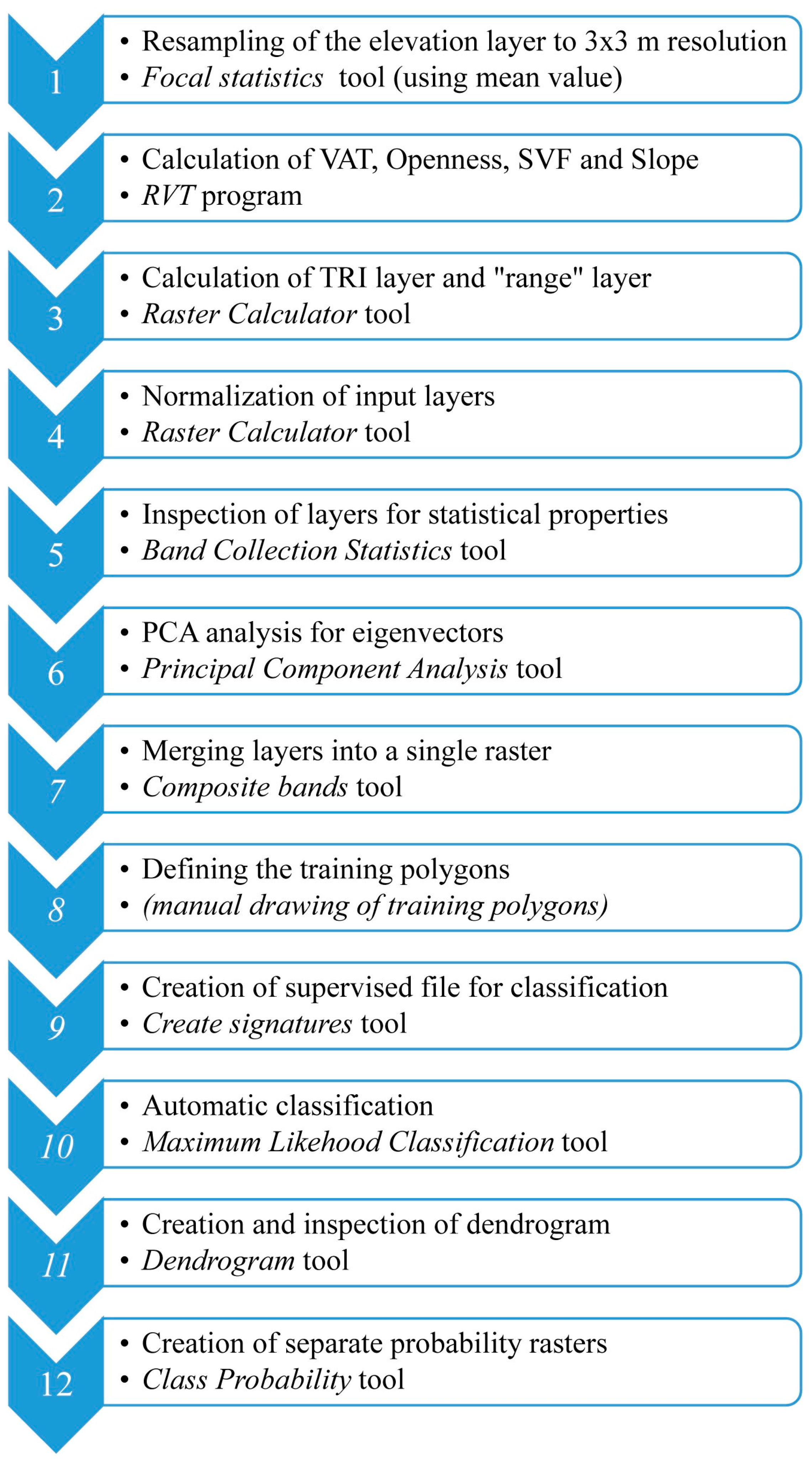
Visualization for Archaeological Topography (VAT layer) [59] was calculated in RVT with default blending preferences. Despite the name of the method, which implies archaeological research, the method itself is not related solely to archeological data as it uses relief (elevation) data for calculations and can be used in any scientific field that deals with visual relief analysis. It has already been successfully used to analyze landslides in the Vipava Valley [35]. VAT is a combination (blending of images) of SVF, Positive Openness, Slope, and HS with default values of blending weights as stated in the program RVT.

Relief Visualization Toolbox is a standalone toolbox that does not require external software to run. It provides a narrow range of methods, and their settings are limited to the most important ones. The selected techniques have been effective regarding the detection of small-scale features, and default values are set to do this task. This software was developed to help scientists visualize raster elevation model datasets. It comprises the following visualization techniques: analytical hillshading and hillshading from multiple directions, PCA of hillshading, slope, Local Relief Model, Sky-View Factor, anisotropic Sky-View Factor, Positive and Negative Openness, Sky Illumination, Local Dominance, and the blended layer of VAT [67].

2.3. Workflow

The workflow is presented in Figure 2 as a sequence of performed commands (tools) in ArcGIS and RVT software. The workflow follows the techniques for supervised classification that were described in the image classification chapter [57]. After resampling and creating the above layers (steps 1 to 3), all layers were normalized to values from 0 to 1 prior to Principal Component Analysis (PCA) (step 4) and analyzed for their statistical properties using the Band Collection Statistics tool (step 5). In step 6, PCA was performed to obtain the eigenvalues that were used to examine the strength of the influence of each layer (see the Results section). Later, the individual single band layers were merged into a multiband layer using the Composite Bands tool (step 7) to facilitate further calculations in ArcGIS. Based on the geological map, training polygons (step 8) were drawn at the locations of typical litho-geomorphological units to identify the following five geological classes: (i) alluvial deposits, (ii) steep carbonate cliffs, (iii) flysch, (iv) Trnovo carbonate plateau, and (v) slope deposits. The latter class includes various slope sediments of recent carbonate scree, gravel and breccias, and older (fossil) landslide deposits ranging from rock avalanches to complex landslides. Compared with the previously used method [34], the class of Karst carbonate plateau was not used because the automatically classified values of Karst plateau interfered with flysch sites on the slopes. This was recognized as unrealistic in the original publication, so this class was omitted from this study. The Karst plateau does not occur at all in the studied area on the northern slopes of the valley where landslides occur.

The training polygons were the same as those used in the original method [34]. Based on these polygons, a signature file was defined for further supervised classification by the Create Signatures tool (step 9). This tool uses samples to define statistical relationships and then writes class definitions in a signature file. This file is also used later to construct a hierarchical clustering method to create a dendrogram. Automatic classification was then performed using Maximum Likelihood Classification (step 10). This tool automatically assigns all unknown cells in the map to the class they most likely belong to. It is possible for a cell to not be assigned to any class, and this is possible due to the stated rejection fraction value, which can be set to 0%, 0.5%, 1%, 2.5%, 5%, etc., up to 99.5%. We used a relatively strict rejection value of 1%. In the next step (11), the relationship between geological classes was tested by inspecting a dendrogram, which is defined as a plot that shows the attribute distances between each pair of sequentially merged classes in the multivariate statistical method of hierarchical clustering. Finally, the Class Probability tool (step 12) was used to analyze the probability value of the occurrence of each litho-geomorphological unit, i.e., how correctly it was classified. The tool therefore assigns the probability of belonging to a unit to each raster cell. Some of the regions identified with MLC were then compared with the four different mapped areas to test the method. The areas were selected to encompass a geologically diverse terrain.

The final result of this image processing protocol was a composite image of all five litho-geomorphological units. Each cell in this raster image corresponded to the prevailing unit with the greatest probability value that appeared on the map. The individual probabilities were examined using the results of the Class Probability tool, which provided five different raster images (one file per unit), and each file contained probability values ranging from 0% to 100%. Since interpreting the results would require switching between five different layers to find the layer with the highest probability of occurrence, it was easier to combine all layers into a composite image containing only the cells of the unit with the highest probability of occurrence.

3. Results

Figure 3 shows the results of Maximum Likelihood Classification method for the entire Vipava Valley region. This computer-generated image, which includes all five geological classes, generally predicts the litho-geomorphological units very well. The alluvium deposits appear correctly on the valley floor, the carbonates of the Trnovo Plateau are visible with high elevation in the northern part, and the carbonate cliffs are correctly predicted on the steep slopes where the carbonates are overthrust over the flysch. However, as noted in the original method [34], the MLC method had problems distinguishing between flysch and slope deposits on the slopes because these two classes sometimes overlap (i.e., the green and blue colors in Figure 3). This correlation is also confirmed by dendrograms (Figure 4), where both classes are closest to each other and consequently the most correlated, which means that they are the most difficult to distinguish from each other. Slope deposits and flysch are connected by the smallest distance; that is, they are the most similar and difficult to distinguish. The alluvium, on the other hand, joins the latest and is therefore the unit that is the most distinct from all the others. The revised method does a better job of distinguishing between units; for example, the dendrogram distance between the slope deposits and the flysch is 0.98 in the original method and twice that (1.90) in the revised method. The revised method also differentiates the other units more effectively because the dendrogram distances are greater for all units.

To some extent, it is understandable that the method has problems with these two units, since these two geological units also overlap in the field. Slope deposits are occasionally deposited as very thin covers over the flysch and sometimes occur as “tongues” of scree material over the flysch formation downslope, which creates very irregular sedimentary bodies. Therefore, these slope sediments should be mapped accurately and carefully.

Nevertheless, the revised method presented in this paper predicts slope sediments much better than the original method [34]. This can be clearly seen in Figure 5, where two examples of enlarged areas with landslides are shown. Figure 5 shows the mapped area with the results of the original and the current (revised) MLC method. Some areas are blank because the field map is not yet fully completed, but the missing areas do not affect the results because they do not contain major landslides that are addressed in this work. The newer method works better because it better predicts the location of flysch. There is also less “interference” and overlap of flysch and slope sediments in all areas.

Within the polygons of the Podrta gora and Gradiška gmajna fossil rock avalanche regions (marked on the map as PG and GG), the locations of fossil landslide deposits (slope sediments) are predicted more accurately. In addition, the recent scree accumulation behind the translational carbonate blocks (e.g., block Stara baba, SB on the map) is now correctly predicted as a slope deposit rather than flysch as before. The other three main units (alluvium, carbonate slopes, and Trnovo karst plateau) are correctly predicted in both cases.

The second example is shown in Figure 6, in the region of the Stogovce landslide (ST on the map). The landslide was triggered in 2010 after a large rainfall event [44,45], and the transported material consisted of clastic sediments of different sizes, mainly gravel and scree that accumulated from steep carbonate slopes in the northwest. Part of this material is still unaffected and lies above the Stogovce landslide. The new method correctly predicts these slope sediments above the landslide and more accurately predicts the already transported material in the body of the landslide. Several scarps in the upper part of the landslide are recognized as steep carbonate slopes, which is somewhat understandable because the scarps are indeed steep. However, scarps are not included in the analysis as a separate training polygon because their spatial extent is too small. In both examples, the areas of flysch and slope deposits are also more homogeneous than in the original method, which is also more realistic.

The number of predicted cells within each landslide area can be calculated and plotted on a bar graph to examine the ratio of slope deposit cells to the total landslide area. The results for the landslides and carbonate blocks mentioned in the above two figures and associated text are shown in Figure 7. It is clear that this method works best for both rock avalanches because the number of slope deposit cells is the highest. For the Stogovce landslide, the predominant class is flysch, and this is also the only area where the revised method yields a greater percentage of flysch than of slope deposits. This is not incorrect since the material in the Stogovce area was actually transported and artificially removed, and the slope deposits (mostly scree and gravel) actually lie as small-scale deposits on top of the flysch (confirmed in several locations in the field). For the translational carbonate block of Stara baba, the number and relative ratio of slope deposit cells are similar for both methods because sediments accumulate behind and on top of the carbonate block, and the class of steep carbonate slopes is also more pronounced because of the steep slopes of dolomite and limestone that form this block. Thus, the improved MLC method works well in this region.

In addition to the examples mentioned above in Figure 5 and Figure 6, we should point out some other novel results. Figure 8 shows the area of the Selo fossil rock avalanche, which was the largest fossil landslide in Slovenia. The large sedimentary body spreads out from the carbonate cliffs and lies fan-shaped in the valley floor. The landslide is more than 42,000 years old, and it looks as if it is composed of two separate landslides [38] that are visible as two separate bodies and fans in Figure 8. Half of the transported volume and consequently the central part of the sedimentary body has already been eroded due to its age. MLC correctly predicts that most of the landslide body consists of carbonate slope sediments overlying flysch. However, the two fans of the landslide are wrongly predicted to be covered with alluvial sediments. In this case, the wrongly predicted ‘alluvium’ can indicate areas of erosion, where scree and mud have been deposited in the bottom of the valley. The latter are classified as alluvium due to their low elevation (the Selo has a typical low H/L ratio of 0.18 [38]) and relatively flat area. It is important to point out a very important difference between Figure 8B,C—in the latter, more deposits are seen in the valley floor.

However, the overall landslide body appears to be less homogeneous and has more predicted flysch areas.

Another example is the region of Rebrnice (Figure 9) in the southeast valley where numerous fossil rock avalanches and recently reactivated landslides occur. These landslides have been mapped as various types of fossil rock and debris slides that overlie older slope deposits and create a complex environment for field mapping. The area is largely covered by carbonate scree, gravel, and breccias overlying highly weathered flysch diluvium at depths between 10 and 60 m where slide plains typically occur [47,48,54]. In this case, the MLC prediction can hardly distinguish between different landslides, which is somewhat expected as the landslides are not typical rotational of translational slip surface events, but deep-seated complex mass movements. The improvement between the former and the newer MLC prediction is the correctness of the prediction of the homogeneity of the carbonate deposits on the slope, especially the areas above the landslides where the carbonate scree accumulates below the cliffs. In the southwest of Figure 9, where mainly flysch occurs on the map, the new MLC prediction is correct because there are no carbonate slope deposits in the field. In general, the new MLC method provides better results for the lithologic units.

4. Discussion

The results show improvements in the automatic classification of the litho-geomorphological units of the Vipava Valley. The obvious improvement is in the homogeneity of the slope deposits and the flysch units, which are less intertwined and overlap less on the maps. As a result, the landslide bodies are easier to identify and much better delineated in the newly created map. This is most likely due to the use of the VAT layer, which has been used in previous work [35] to improve the visualization of slope mass movements by combining four different layers that enhance the shading on a shaded relief raster.

It is important to note that the MLC recognized some slope sediments on the valley floor that overlie the alluvium, although they normally occur at higher elevations, and the alluvium typically occurs in the lowest parts of the valley. This could be explained by the smaller influence of the Elevation Layer on the classification.

A principal component analysis was performed to better understand the correlations between the layers. The PCA also provided important information about the eigenvalues of the layers and which layers explained most of the variance.

4.1. Inspection of Layers

At the beginning, before the MLC was executed, the correlation between the input layers was checked (Figure 10). There is a high positive correlation between the SVF, VAT, and Positive Openness layers. All three methods determine the fraction of the visible sky that is bounded by relief. SVF is one of the input layers for VAT, so the positive correlation is expected. The same is true for Openness, which is known to have a similar problem when determining the horizon as SVF [58]. The strong negative correlation of slope with SVF and VAT is logical because shallow (open) reliefs with low slopes have high VAT and SVF values.

Note the strong correlation between elevation and TRI since the values of the TRI method depend on elevation itself. The squaring of the elevation values mean the results are affected by the absolute elevation value. For example, the 10-m elevation range at lower elevations is different for the same elevation range at higher elevations. Therefore, there is a positive correlation between the layers, and, in our opinion, this method is less suitable for surface roughness analysis than the range method, which has a much lower correlation with the slope values.

4.2. Eigenvalues and Relative Importance of the Layers

The table of eigenvalues and eigenvectors (Figure 11) calculated using the PCA method also provided very informative results. Eigenvalues represent the total amount of variance that can be explained by a particular principal component of the PCA method. Their magnitude is represented by eigenvectors. The larger the values of eigenvalue and eigenvector are, the stronger the influence of the PC layer is. PC layers consist of different original input layers, and their “composition” is represented in each column. For example, the VAT layer has the largest value of the eigenvector in the first column (PC layer 1), which means it is the most “important” layer and explains most of the variance within that layer. The most valuable data in the table are the eigenvalues of the individual PC layers because these provide information regarding which original layer contains the most information about the relief and consequently explains most of the variability in the relief.

From the table, it can be seen that the VAT layer is the most relevant layer and explains almost 43% of the total variability. This is followed by the Aspect and Elevation layers, which together account for 90% of the variance. If we include two other layers (Hillshade and Slope), the cumulative share increases to 99%. Thus, other layers contribute less than 1% to the total variance and the interpretation of the variability of the relief and are therefore not needed for interpretations and/or calculations.

Some of these results are to be expected, to some degree. Positive correlations between the layers (Figure 10), such as VAT, SVF, and Positive Openness mean some of the information used to explain the variance is redundant, and only one of the layers should be used for the calculations. However, it is often questionable which layer should be used and which should be neglected. From the table, it can be seen that using VAT is better than using the similar SVF or Positive Openness because VAT has higher eigenvalues.

Therefore, VAT, Aspect, and Elevation layers are the layers that should be used in the geomorphological calculations of lidar-derived digital elevation models. In this case, the Hillshade, SVF, Positive Openness, and Slope layers should not be used because they comprise the VAT layer; therefore, their use would lead to redundancy in the data. Range is preferable to TRI because it is independent of elevation, and both contribute less than 1% to the total variance. Curvature, on the other hand, has virtually no influence and is also independent of all other layers (the very low importance of this layer was already discussed in the original method [34]).

5. Conclusions

The main findings of this study can be summarized in the following points:

-

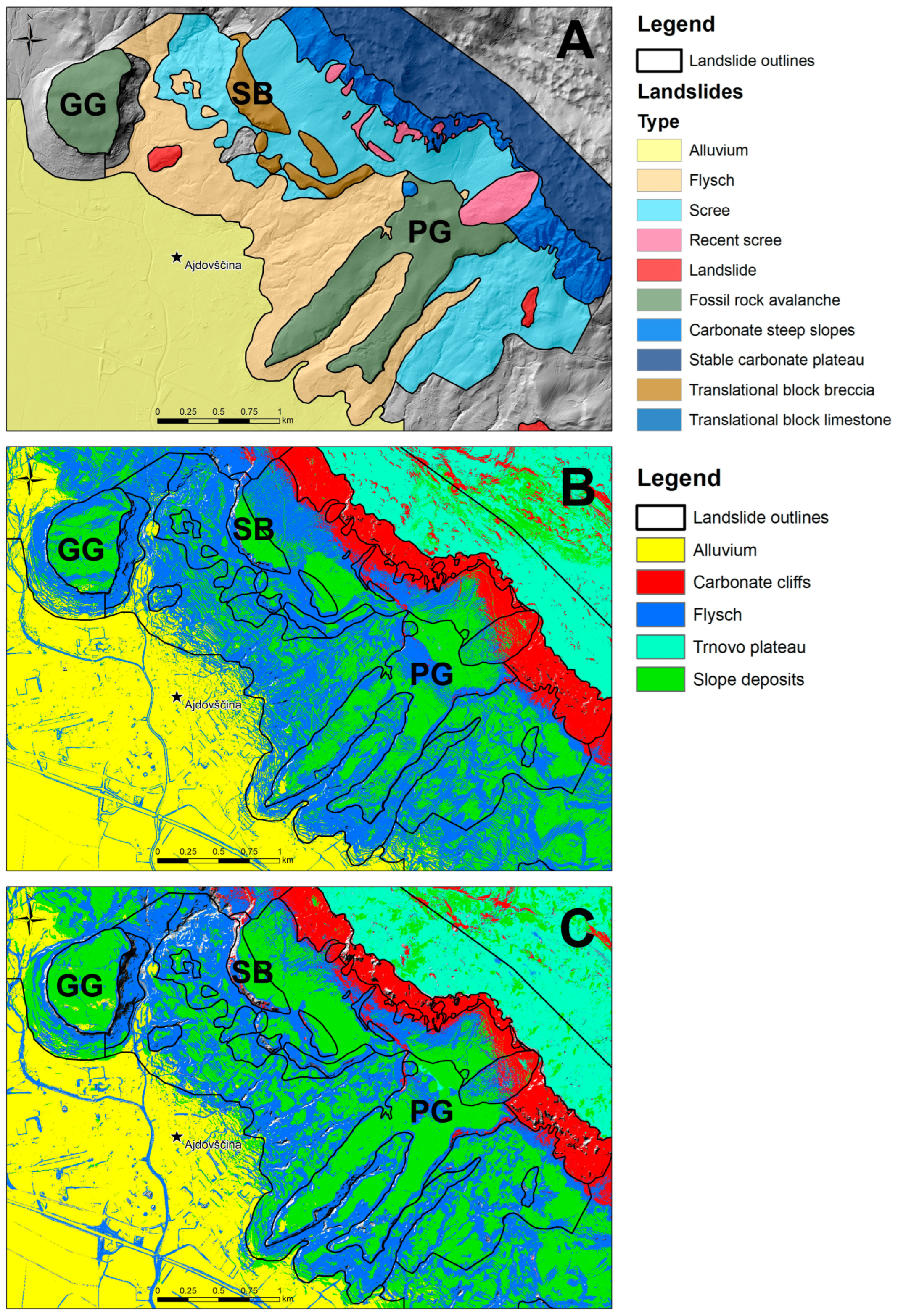
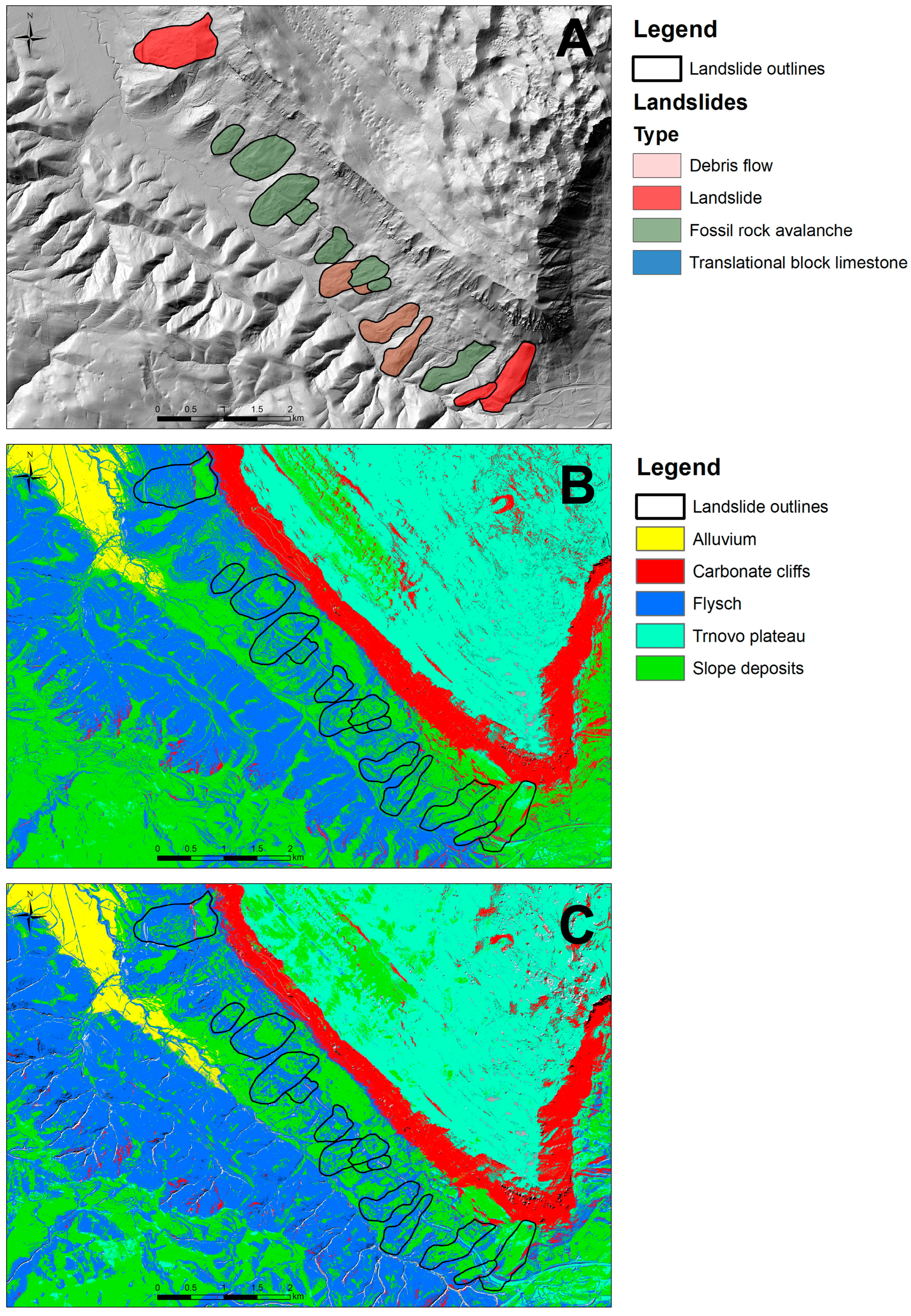
The Maximum Likelihood Classification (MLC) automatic classification technique is useful for delineating various litho-geomorphological units and generally predicts these units very well.

-

The classes that are most easily and correctly recognized and classified are alluvial sediments, high karst plateaus, and steep carbonate slopes, which is confirmed by looking at the dendrogram. The classification algorithm has difficulty distinguishing flysch and slope sediments because they often overlap. However, these sediments are properly “intertwined” in the terrain in the form of complex sedimentary bodies.

-

Quantitative examination of the original and revised dendrograms confirms that the revised method does a much better job of distinguishing between these two units. The revised method also distinguishes between other units well because the dendrogram distances are larger for all units. The number of correctly predicted pixels is also larger in the case of the revised method for the areas of rock avalanches, as shown in the comparison of the bar graphs.

-

Scarps of landslides are also well recognized, but due to their small spatial extent, it was not possible to study this class separately. We propose including this morphological feature of landslides when a larger data set is available.

-

Compared with the original method with fewer input layers, the revised approach with the addition of the DEM-derived geomorphological raster layers VAT, Sky View Factor, Openness, and others provides much better prediction of the slope sediments.

-

Among these layers, VAT should be used instead of Sky View Factor or Openness because it encompasses these two layers of information and is recognized by multivariate statistics as the “most important” layer with the highest eigenvalues; thus, it contributes the most to explaining variance. In addition, strong correlations exist between VAT, Sky View Factor, and Openness, and the use of more than one of these layers together in the analyses is not recommended because of redundancy in the data. Therefore, correlations should be checked before using multilayer analyses.

-

The VAT layer, which is a blended image that includes Hillshade, Slope, Sky View Factor, and Positive Openness, proves an added value to the automatic classification of various litho-geomorphological units since it explains most of the variance and improves the classification of two overlapping units—slope sediments and flysch.

-

The independent layers VAT, Aspect, and Elevation explain a large amount (90%) of the total variance.

-

The use of Range rather than TRI is preferable because of the dependence of TRI on the elevation values.

-

We see our method’s advantage in its wide data availability and the simplicity of its application—only a Digital Elevation Model (DEM) is needed, from which all input layers are derived. Certainly, the computer-generated image is not intended as a substitute for traditional mapping methods, but it has proven very useful for predicting landslide deposits before field mapping is performed.

-

Although this methodology might not be appropriate for other and more complex geological settings, we encourage researchers to use the additional geomorphological DEM-derived rasters and blended images in spatial analyses of landslides along with more familiar layers such as Slope, Hillshade, Aspect, and Curvature layers.

References

1. Canavesi, V.; Segoni, S.; Rosi, A.; Ting, X.; Nery, T.; Catani, F.; Casagli, N. Different Approaches to Use Morphometric Attributes in Landslide Susceptibility Mapping Based on Meso-Scale Spatial Units: A Case Study in Rio de Janeiro (Brazil). Remote Sens. 2020, 12, 1826. [Google Scholar] [CrossRef]
2. Frodella, W.; Rosi, A.; Spizzichino, D.; Nocentini, M.; Lombardi, L.; Ciampalini, A.; Vannocci, P.; Ramboason, N.; Margottini, C.; Tofani, V.; et al. Integrated approach for landslide hazard assessment in the High City of Antananarivo, Madagascar (UNESCO tentative site). Landslides 2022, 19, 2685–2709. [Google Scholar] [CrossRef]
3. Maxwell, A.E.; Shobe, C.M. Land-surface parameters for spatial predictive mapping and modeling. Earth-Sci. Rev. 2022, 226, 103944. [Google Scholar] [CrossRef]
4. Baeza, C.; Corominas, J. Assessment of shallow landslide susceptibility by means of statistical techniques. In Proceedings of the Seventh International Symposium on Landslides, Trondheim, Norway, 17–21 June 1996; Volume 1, pp. 147–152. [Google Scholar]
5. Park, N.W.; Chi, K.H. Quantitative assessment of landslide susceptibility using high-resolution remote sensing data and a generalized additive model. Int. J. Remote Sens. 2008, 29, 247–264. [Google Scholar] [CrossRef]
6. Yilmaz, I. Landslide susceptibility mapping using frequency ratio, logistic regression, artificial neural networks and their comparison: A case study from Kat landslides (Tokat—Turkey). Comput. Geosci. 2009, 35, 1125–1138. [Google Scholar] [CrossRef]
7. Manzo, G.; Tofani, V.; Segoni, S.; Battistini, A.; Catani, F. GIS techniques for regional-scale landslide susceptibility assessment: The Sicily (Italy) case study. Int. J. Geogr. Inf. Sci. 2013, 27, 1433–1452. [Google Scholar] [CrossRef]
8. Kavzoglu, T.; Sahin, E.K.; Colkesen, I. Landslide susceptibility mapping using GIS-based multi-criteria decision analysis, support vector machines, and logistic regression. Landslides 2014, 11, 425–439. [Google Scholar] [CrossRef]
9. Leshchinsky, B.A.; Olsen, M.J.; Tanyu, B.F. Contour Connection Method for automated indentification and classification of landslide deposits. Comput. Geosci. 2014, 74, 27–38. [Google Scholar] [CrossRef]
10. Knevels, R.; Petschko, H.; Leopold, P.; Brenning, A. Geographic Object-Based Image Analysis for Automated Landslide Detection Using Open Source GIS Software. ISPRS In. J. Geo-Inf. 2019, 8, 551. [Google Scholar] [CrossRef] [Green Version]
11. Liu, Y.; Zhao, L.; Bao, A.; Li, J.; Yan, X. Chinese High Resolution Satellite Data and GIS-Based Assessment of Landslide Susceptibility along Highway G30 in Guozigou Valley Using Logistic Regression and MaxEnt Model. Remote Sens. 2022, 14, 3620. [Google Scholar] [CrossRef]
12. Medina, V.; Hürlimann, M.; Guo, Z.; Lloret, A.; Vaunat, J. Fast physically-based model for rainfall-induced landslide susceptibility assessment at regional scale. Catena 2021, 201, 105213. [Google Scholar] [CrossRef]
13. Fang, Z.; Wang, Y.; Peng, L.; Hong, H. Integration of convolutional neural network and conventional machine learning classifiers for landslide susceptibility mapping. Comput. Geosci. 2020, 139, 104470. [Google Scholar] [CrossRef]
14. Janušaitė, R.; Jukna, L.; Jarmalavičius, D.; Pupienis, D.; Žilinskas, G. A Novel GIS-Based Approach for Automated Detection of Nearshore Sandbar Morphological Characteristics in Optical Satellite Imagery. Remote Sens. 2021, 13, 2233. [Google Scholar] [CrossRef]
15. Lin, S.; Chen, N.; He, Z. Automatic Landform Recognition from the Perspective of Watershed Spatial Structure Based on Digital Elevation Models. Remote Sens. 2021, 13, 3926. [Google Scholar] [CrossRef]
16. Yang, Z.; Wei, J.; Deng, J.; Zhao, S. An Improved Method for the Evaluation and Local Multi-Scale Optimization of the Automatic Extraction of Slope Units in Complex Terrains. Remote Sens. 2022, 14, 3444. [Google Scholar] [CrossRef]
17. Zhou, Y.; Wang, H.; Yang, R.; Yao, G.; Xu, Q.; Zhang, X. A Novel Weakly Supervised Remote Sensing Landslide Semantic Segmentation Method: Combing CAM and cycleGAN Algorithms. Remote Sens. 2022, 14, 3650. [Google Scholar] [CrossRef]
18. Xun, Z.; Zhao, C.; Kang, Y.; Liu, X.; Liu, Y.; Du, C. Automatic Extraction of Potential Landslides by Integrating an Optical Remote Sensing Image with an InSAR-Derived Deformation Map. Remote Sens. 2022, 14, 2669. [Google Scholar] [CrossRef]
19. Martha, T.; Kerle, N.; Jetten, V.; Westen, C.J.; Kumar, K.V. Characterising Spectral, Spatial and Morphometric Properties of Landslides for Semi-automatic Detection Using Object-oriented Methods. Geomorphology 2010, 116, 24–36. [Google Scholar] [CrossRef]
20. Guzzetti, F.; Mondini, A.C.; Cardinali, M.; Fiorucci, F.; Santangelo, M.; Chang, K.-T. Landslide inventory maps: New tools for an old problem. Earth-Sci. Rev. 2012, 112, 42–66. [Google Scholar] [CrossRef] [Green Version]
21. Van Den Eeckhaut, M.; Kerle, N.; Poesen, J.; Hervás, J. Object-oriented identification of forested landslides with derivatives of single pulse LiDAR data. Geomorphology 2012, 173–174, 30–42. [Google Scholar] [CrossRef]
22. Chen, W.; Li, X.; Wang, Y.; Chen, G.; Liu, S. Forested landslide detection using LiDAR data and the random forest algorithm: A case study of the Three Gorges, China. Remote Sens. Environ. 2014, 152, 291–301. [Google Scholar] [CrossRef]
23. Pawłuszek, K.; Borkowski, A. Automatic landslides mapping in the principal component domain. In 4th World Landslide Forum Proceedings; Advancing Culture of Living with Landslides, Landslides in Different Environments; Mikoš, M., Vilímek, V., Yin, Y., Sassa, K., Eds.; Springer Nature Publishing: Cham, Switzerland, 2017; Volume 5, pp. 412–428. [Google Scholar] [CrossRef]
24. Pawłuszek, K.; Borkowski, A.; Tarolli, P. Towards the optimal pixel size of DEM for automatic mapping of landslide areas. Int. Arch. Photogramm. Remote Sens. Spat. Inf. Sci. ISPRS Hann. Workshop 2017, XLII-1/W1, 83–90. [Google Scholar] [CrossRef] [Green Version]
25. Mondini, A.C.; Guzzetti, F.; Reichenbach, P.; Rossi, M.; Cardinali, M.; Ardizzone, F. Semi-automatic recognition and mapping of rainfall induced shallow landslides using optical satellite images. Remote Sens. Environ. 2011, 115, 1743–1757. [Google Scholar] [CrossRef]
26. Mondini, A.C.; Marchesini, I.; Rossi, M.; Chang, K.-T.; Pasquariello, G.; Guzzetti, F. Bayesian framework for mapping and classifying shallow landslides exploiting remote sensing and topographic data. Geomorphology 2013, 201, 135–147. [Google Scholar] [CrossRef]
27. Mondini, A.C.; Chang, K.-T.; Chiang, S.-H.; Schlögel, R.; Notarnicola, C.; Saito, H. Automatic mapping of event landslides at basin scale in Taiwan using a Montecarlo approach and synthetic land cover fingerprints. Int. J. Appl. Earth. Obs. Geoinf. 2017, 63, 112–121. [Google Scholar] [CrossRef]
28. Comert, R.; Avdan, U.; Gorum, T.; Nefeslioglu, H.A. Mapping of shallow landslides with object-based image analysis from unmanned aerial vehicle data. Eng. Geol. 2019, 260, 105264. [Google Scholar] [CrossRef]
29. Yu, B.; Chen, F.; Xu, C. Landslide detection based on contour-based deep learning framework in case of national scale of Nepal in 2015. Comput. Geosci. 2020, 135, 104388. [Google Scholar] [CrossRef]
30. Yang, S.; Wang, Y.; Wang, P.; Mu, J.; Jiao, S.; Zhao, X.; Wang, Z.; Wang, K.; Zhu, Y. Automatic Identification of Landslides Based on Deep Learning. Appl. Sci. 2022, 12, 8153. [Google Scholar] [CrossRef]
31. Danneels, G.; Pirard, E.; Havenith, H.-B. Automatic landslide detection from remote sensing images using supervised classification methods. In Proceedings of the IEEE IGARSS, Barcelona, Spain, 23–27 July 2007; pp. 3014–3017. [Google Scholar] [CrossRef]
32. Amato, G.; Palombi, L.; Raimondi, V. Data–driven classification of landslide types at a national scale by using Artificial Neural Networks. Int. J. Appl. Earth. Obs. Geoinf. 2021, 104, 102549. [Google Scholar] [CrossRef]
33. Yu, L.; Porwal, A.; Holden, E.-J.; Dentith, M.C. Towards automatic lithological classification from remote sensing data using support vector machines. Comp. Geosci. 2012, 45, 229–239. [Google Scholar] [CrossRef]
34. Verbovšek, T.; Popit, T. GIS-assisted classification of litho-geomorphological units using Maximum Likelihood Classification, Vipava Valley, SW Slovenia. Landslides 2018, 15, 1415–1424. [Google Scholar] [CrossRef]
35. Verbovšek, T.; Popit, T.; Kokalj, Ž. VAT Method for Visualization of Mass Movement Features: An Alternative to Hillshaded DEM. Remote Sens. 2019, 11, 2946. [Google Scholar] [CrossRef]
36. Komac, M.; Ribičič, M. Landslide susceptibility map of Slovenia at scale 1:250,000. Geologija 2006, 49, 295–309. [Google Scholar] [CrossRef]
37. Popit, T.; Supej, B.; Kokalj, Ž.; Verbovšek, T. Comparison of methods for geomorphometric analyzes of surface roughness in the Vipava Valley. Geod. Vestn. 2016, 60, 227–240. [Google Scholar] [CrossRef]
38. Verbovšek, T.; Košir, A.; Teran, M.; Zajc, M.; Popit, T. Volume determination of the Selo landslide complex (SW Slovenia): Integrating field mapping, ground penetrating radar and GIS approaches. Landslides 2017, 14, 1265–1274. [Google Scholar] [CrossRef]
39. Kočevar, M.; Ribičič, M. Geological, hydrogeological and geomechanical investigation of Slano blato landslide. Geologija 2002, 45, 427–432. [Google Scholar] [CrossRef]
40. Ribičič, M. Calculation of the moving landslide masses volume from air images. Geologija 2003, 46, 413–418. [Google Scholar]
41. Logar, J.; Fifer Bizjak, K.; Kočevar, M.; Mikoš, M.; Ribičič, M.; Majes, B. History and present state of the Slano blato landslide. Nat. Hazards Earth Syst. Sci. 2005, 5, 447–457. [Google Scholar] [CrossRef] [Green Version]
42. Placer, L.; Jež, J.; Atanackov, J. Structural aspect of the Slano blato landslide (Slovenia). Geologija 2008, 51, 229–234. [Google Scholar] [CrossRef]
43. Fifer Bizjak, K.; Zupančič-Valant, A. Site and laboratory investigation of the Slano blato landslide. Eng. Geol. 2009, 105, 171–185. [Google Scholar] [CrossRef]
44. Petkovšek, A.; Maček, M.; Mikoš, M.; Majes, B. Mechanisms of Active Landslides in Flysch. In Landslides: Global Risk Preparedness, Chapter 10; Sassa, K., Rouhban, B., McSaveney, M., He, B., Eds.; Springer: Berlin/Heidelberg, Germany, 2013; pp. 149–165. [Google Scholar] [CrossRef]
45. Petkovšek, A.; Fazarinc, R.; Kočevar, M.; Maček, M.; Majes, B.; Mikoš, M. The Stogovce landslide in SW Slovenia triggered during the September 2010 extreme rainfall event. Landslides 2011, 8, 499–506. [Google Scholar] [CrossRef]
46. Verbovšek, T.; Kočevar, M.; Benko, I.; Maček, M.; Petkovšek, A. Monitoring of the Stogovce landslide slope movements with GEASENSE GNSS probes. In 4th World Landslide Forum Proceedings, Ljubljana, Slovenia, 30 May to 2 June 2017. Advancing Culture of Living with Landslides, Landslides in Different Environments; Advances in Landslide Technology; Springer Nature Publishing: Cham, Switzerland, 2017; Volume 3, pp. 311–319. [Google Scholar] [CrossRef]
47. Popit, T.; Rožič, B.; Šmuc, A.; Kokalj, Ž.; Verbovšek, T.; Košir, A. A lidar, GIS and basic spatial statistic application for the study of ravine and palaeo-ravine evolution in the upper Vipava Valley, SW Slovenia. Geomorphology 2014, 204, 638–645. [Google Scholar] [CrossRef]
48. Popit, T. Origin of planation surfaces in the hinterland of Šumljak sedimentary bodies in Rebrnice (Upper Vipava Valley, SW Slovenia). Geologija 2017, 60, 297–307. [Google Scholar] [CrossRef]
49. Kocjančič, M.; Popit, T.; Verbovšek, T. Gravitational sliding of the carbonate megablocks in the Vipava Valley, SW Slovenia. Acta Geogr. Slov. 2019, 59, 7–22. [Google Scholar] [CrossRef] [Green Version]
50. Jemec Auflič, M.; Jež, J.; Popit, T.; Košir, A.; Maček, M.; Logar, J.; Petkovšek, A.; Mikoš, M.; Calligaris, C.; Boccali, C.; et al. The variety of landslide forms in Slovenia and its immediate NW surroundings. Landslides 2017, 14, 1537–1546. [Google Scholar] [CrossRef]
51. Buser, S. Basic Geological Map of SFR Yugoslavia 1:100,000, Sheet Gorica L 33–78; Federal Geological Survey: Belgrade, Republic of Serbia, 1973. [Google Scholar]
52. Placer, L. Geologic structure of south-western Slovenia. Geologija 1981, 24, 27–60. [Google Scholar]
53. Jurkovšek, B.; Biolchi, S.; Furlani, S.; Kolar-Jurkovšek, T.; Zini, L.; Jež, J.; Tunis, G.; Bavec, M.; Cucchi, F. Geology of the classical karst region (SW Slovenia–NE Italy). J. Maps 2013, 12, 352–362. [Google Scholar] [CrossRef] [Green Version]
54. Jež, J. Reasons and mechanism for soil sliding processes in the Rebrnice area, Vipava Valley, SW Slovenia. Geologija 2007, 50, 55–63. [Google Scholar] [CrossRef]
55. Novak, A.; Popit, T.; Verbovšek, T. Heterogeneously composed Lozice fossil landslide in Rebrnice area, Vipava Valley. Geologija 2017, 60, 145–155. [Google Scholar] [CrossRef]
56. Buser, S.; Grad, K.; Pleničar, M. Basic geological Map of SFR Yugoslavia 1:100,000, Sheet Postojna L 33–77; Federal Geological Survey: Belgrade, Republic of Serbia, 1967. [Google Scholar]
57. ESRI Inc. Working with ArcGIS Spatial Analyst; ESRI Educational Services: Redlands, CA, USA, 2007. [Google Scholar]
58. Zakšek, K.; Oštir, K.; Kokalj, Ž. Sky-View Factor as a Relief Visualization Technique. Remote Sens. 2011, 3, 398–415. [Google Scholar] [CrossRef] [Green Version]
59. Kokalj, Ž.; Somrak, M. Why Not a Single Image? Combining Visualizations to Facilitate Fieldwork and On-Screen Mapping. Remote Sens. 2019, 11, 747. [Google Scholar] [CrossRef] [Green Version]
60. Lo, C.M.; Lee, C.F.; Keck, J. Application of sky view factor technique to the interpretation and reactivation assessment of landslide activity. Environ. Earth Sci. 2017, 76, 375. [Google Scholar] [CrossRef]
61. Yokoyama, R.; Shlrasawa, M.; Pike, R.J. Visualizing topography by openness: A new application of image processing to digital elevation models. Photogramm. Eng. Remote Sens. 2002, 68, 251–266. [Google Scholar]
62. Doneus, M. Openness as Visualization Technique for Interpretative Mapping of Airborne Lidar Derived Digital Terrain Models. Remote Sens. 2013, 5, 6427–6442. [Google Scholar] [CrossRef] [Green Version]
63. Li, J.; Zhang, H.; Xu, E. A two-level nested model for extrating positive and negative terrains combining morpholoy and visualization indicators. Ecol. Indic. 2020, 109, 105842. [Google Scholar] [CrossRef]
64. Riley, S.J.; DeGloria, S.D.; Elliot, R. A terrain ruggedness index that quantifies topographic heterogeneity. Intermt. J. Sci. 1999, 5, 23–27. [Google Scholar]
65. Popit, T.; Verbovšek, T. Analysis of surface roughness in the Sveta Magdalena paleo-landslide in the Rebrnice area. RMZ-Mater. Geoenvironment 2013, 60, 197–204. [Google Scholar]
66. Popit, T.; Rožič, B.; Šmuc, A.; Novak, A.; Verbovšek, T. Using a lidar-based height variability method for recognizing and analyzing fault displacement and related fossil mass movement in the Vipava Valley, SW Slovenia. Remote Sens. 2022, 14, 2016. [Google Scholar] [CrossRef]
67. Kokalj, Ž.; Hesse, R. Airborne laser scanning raster data visualization. In A Guide to Good Practice; Prostor, kraj, čas 14; ZRC Publishing house: Ljubljana, Republic of Slovenia, 2017. [Google Scholar] [CrossRef]
Figure 2. Workflow process for the automatic supervised classification. The first line denotes the description and purpose of the tool, and the second line includes the name of the tool used in ArcGIS.
Remotesensing 15 00531 g002
Figure 3. General map of the MLC prediction.
Remotesensing 15 00531 g003
Figure 4. Comparison of the original and revised MLC method results. (A) dendrogram of the revised MLC method, and (B) dendrogram of the original MLC method.
Remotesensing 15 00531 g004
Figure 5. Podrta gora area. (A) outlines and main sediments of the landslides and litho-geomorphological units; (B) original MLC results [34]; and (C) results from this study.
Remotesensing 15 00531 g005
Figure 6. Stogovce landslide area. (A) outlines and main sediments of the litho-geomorphological units; (B) original MLC results; and (C) results from this study.
Remotesensing 15 00531 g006
Figure 7. Bar chart comparison of the percentages of predicted units in the areas of landslides Stogovce, rock avalanches Podrta gora and Gradiška gmajna, and translational carbonate block Stara baba. ORG = original MLC method and REV = revised MLC method.
Remotesensing 15 00531 g007
Figure 8. Selo landslide area. (A) outlines and main sediments of the litho-geomorphological units; (B) original MLC results; and (C) results from this study.
Remotesensing 15 00531 g008
Figure 9. Rebrnice landslide area. (A) outlines and main sediments of the litho-geomorphological units; (B) original MLC results; and (C) results from this study.
Remotesensing 15 00531 g009
Figure 10. Correlation coefficients (r) among the input layers. The green color indicates a directly proportional correlation, and the red color indicates an inversely proportional correlation between the layers (the darker color, the stronger the correlation).
Remotesensing 15 00531 g010
Figure 11. Eigenvalues and eigenvectors of the input layers. The intensity of the color indicates a higher ratio of eigenvalues.
Remotesensing 15 00531 g011
Disclaimer/Publisher’s Note: The statements, opinions and data contained in all publications are solely those of the individual author(s) and contributor(s) and not of MDPI and/or the editor(s). MDPI and/or the editor(s) disclaim responsibility for any injury to people or property resulting from any ideas, methods, instructions or products referred to in the content.