Article

Parallel Computation of Multi-GNSS and Multi-Frequency Inter-Frequency Clock Biases and Observable-Specific Biases

1
School of Geodesy and Geomatics, Wuhan University, Wuhan 430079, China
2
Institute of Surveying and Mapping, Information Engineering University, Zhengzhou 450001, China
3
College of Computer and Information, Hohai University, Nanjing 211100, China
*
Authors to whom correspondence should be addressed.
Remote Sens. 2023, 15(7), 1953; https://doi.org/10.3390/rs15071953
Submission received: 26 March 2023 / Revised: 1 April 2023 / Accepted: 3 April 2023 / Published: 6 April 2023
(This article belongs to the Special Issue Precise Point Positioning with GPS, GLONASS, BeiDou, and Galileo II)

Abstract

:
With the widespread application of GNSS, the delicate handling of biases among different systems and different frequencies is of critical importance, wherein the inter-frequency clock biases (IFCBs) and observable-specific signal biases (OSBs) should be carefully corrected. Usually, a serial approach is used to calculate these products. To accelerate the computation speed and reduce the time delay, a multicore parallel estimation strategy for IFCBs, code, and phase OSBs by utilizing task parallel library (TPL) is proposed, the parallel computations, including precise point positioning (PPP), IFCBs, and OSBs estimation, being carried out on the basis of data parallelisms and task-based asynchronous programming. Three weeks of observables from the multi-GNSS experiment campaign (MGEX) network is utilized. The result shows that the IFCB errors of GPS Block IIF and GLONASS M+ satellites are nonnegligible, in which the GLONASS M+ satellite R21 shows the largest IFCB of more than 0.60 m, while those of other systems and frequencies are marginal, and the code OSBs present excellent stability with a standard deviation (STD) of 0.10 ns for GPS and approximately 0.20 ns for other satellite systems. Besides, the phase OSBs of all systems show the stability of better than 0.10 ns, wherein the Galileo satellites show the best performance of 0.01 ns. Compared with the single-core serial computing method, the acceleration rates for IFCBs and OSBs estimation are 3.10, 5.53, 9.66, and 17.04 times higher using four, eight, sixteen, and thirty-two physical cores, respectively, through multi-core parallelized execution.

1. Introduction

With the continuous development and upgrade of GPS, GLONASS, Galileo, BeiDou navigation satellite system (BDS), and other regional and augmentation systems, more than 140 navigation satellites can transmit triple frequencies, and even more signals [1]. On the one hand, the advantages of multiple systems and multiple frequencies provided by global navigation satellite systems (GNSS) are noticeable in the aspects of positioning accuracy, convergence speed, availability, and reliability. On the other hand, the combined usage of multiple frequencies and unified model processing at the observation level can effectively enhance the performance of multi-GNSS services [2].
To achieve those improvements of the positioning performance, the biases handling among different systems and different frequencies is inevitable. In addition to solving those biases as parameters to be estimated in the normal equation, two kinds of products are commonly estimated and broadcast currently. One is to process the biases using a differential approach, i.e., inter-frequency bias (IFB), inter-system bias (ISB), and differential code bias (DCB), in the satellite [3] and receive side [4], a combination mode, i.e., uncalibrated phase delay (UPD) in the satellite side [5] and receiver side [6] and inter-frequency clock biases (IFCB). On the condition of multiple frequencies, the existing biases’ calibrations are too complicated to extend to different frequencies and signal modulations [7], and, in view of the increasing number of bias combinations, how to provide users with a uniform and convenient bias correction method is also a key issue that needs to be urgently addressed. Hence, different from differential form and combination, a more effective and efficient approach to deal with the code and phase deviations is the concept of observable-specific signal biases (OSBs); the OSBs clearly depict and define the deviations of each code and phase observations, making the deviations disposal of multiple systems and multiple frequencies more flexible and convenient [8,9]. The OSB format was proposed and developed by Schaer et al. [10,11]. The OSB product consists of a correction for each channel’s pseudorange and carrier phase signal, and the user simply removes the respective deviation from the original observation [12,13]. Li et al. [14] proposed a unified strategy of OSBs’ estimation and correction model for undifferenced ambiguity fixing of multiple systems and multiple frequencies, but global ionosphere maps (GIM) are necessary for code OSBs’ estimation. Currently, several institutions, including the Centre National d’Etudes Spatiales (CNES), the Center for Orbit Determination in Europe (CODE), the Chinese Academy of Sciences (CAS), and Wuhan University, can provide daily OSBs per satellite. All those products support multi-GNSS and multi-frequency, and they differ from each other in the aspect of publishment latency, i.e., Wuhan University provides rapid products, and CNES can broadcast both real-time and post products. Additionally, since the phase ambiguities can only take in a constant part of carrier phase biases, the combination of the time-varying aspect of phase biases of triple-frequency observations, which is named as IFCB [15], should also be carefully corrected. It is worth mentioning that whether the estimation is for OSBs or IFCBs, a large-scale GNSS network with hundreds of reference stations is utilized to obtain those products.
Usually, serial computing is typically applied in the estimation of those products, and multi-GNSS and multi-frequency data from regional or huge global GNSS networks are solved serially, wherein the IFCBs, code, and phase OSBs are estimated in turn. With the rapid development of numerous parallel computing technologies and multicore platforms, parallelized decomposition of computationally intensive operations and multicore distributed processing of data-intensive solving can effectively improve the speed of GNSS solving. As early as 2010, the first working group of the International Association of Geodesy (IAG) launched the Dancer program, which was designed to rapidly solve original observation data from the level of observation equation for the space geodesy [16], and corresponding achievements were applied to the international terrestrial reference frame (ITRF) reprocessing and upgrade task. Using open multi-processing (OpenMP) to accelerate the covariance update process, Kuang et al. [17] realized the real-time GPS satellite ephemeris computation. Li et al. [18] developed a parallel estimation approach for GNSS network corrections using the undifferenced ionospheric-free (IF) combination, wherein the real-time FCBs and tropospheric delays parallel estimation, and tropospheric modelings were implemented concurrently. Chen et al. [19] proposed a parallel algorithm for multi-GNSS orbit determination, and, in the level of normal equation, the guided scheduling and optimal cache memory traffics were performed in a multi-thread way. Additionally, to speed up the GNSS data processing, the software package Bernese 5.0 and its later version, GIPSY [20], GNSSer [21] all supports multi-thread, multi-core, or muti-node parallel computing. Hence, it is feasible to further apply parallel computing into IFCBs’ and OSBs’ estimation.
In this contribution, our aim is to accelerate the estimation process of IFCBs, code, and phase OSBs using multi-core parallel tool task parallel library (TPL), so as to reduce the delay time for publishing precise bias products of multiple systems and multiple frequencies. This manuscript consists of four parts. First, the parallel estimation methodology of IFCBs and OSBs is proposed. Next, the observation data with detailed solving strategy is introduced. Then, the characteristics of IFCBs and OSBs of multi-GNSS are discussed and analyzed, and the computational efficiency is also validated using different numbers of physical cores. Finally, discussions and conclusions are provided.

2. Methodology

The parallel resolution of undifferenced and uncombined PPP of multiple systems and multiple frequencies is introduced first, followed by the parallel estimation method of IFCBs, and, finally, the parallel computing of code and phase OSBs is given.

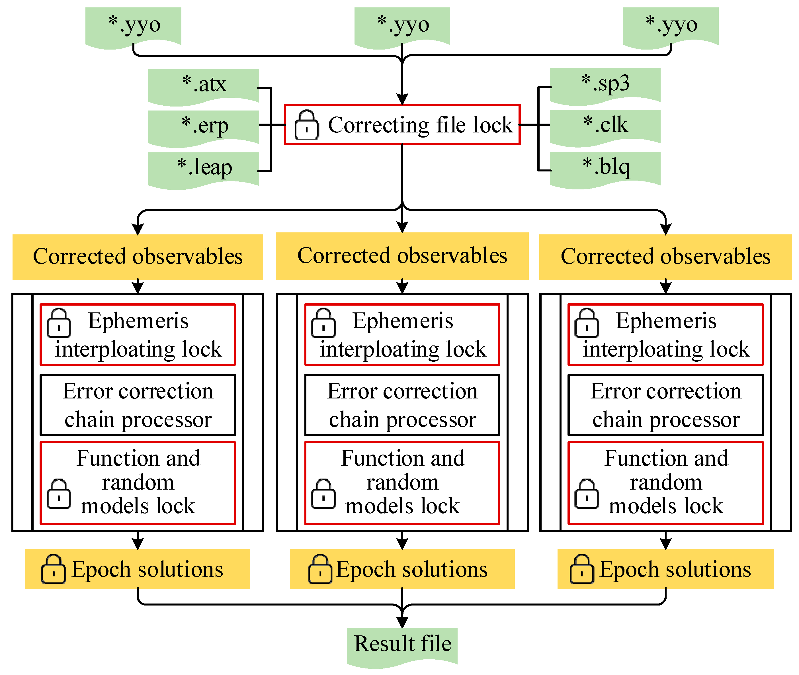
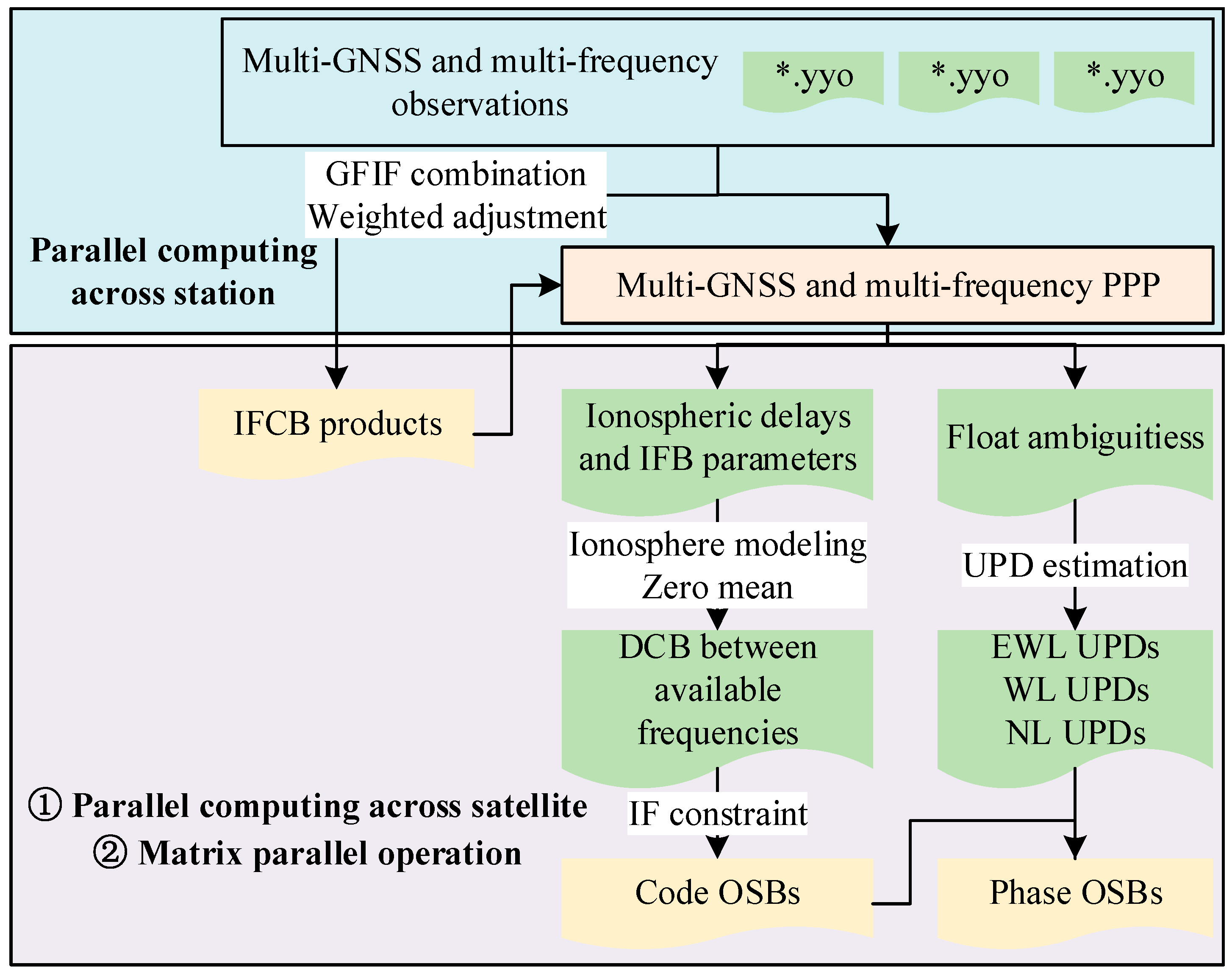
2.1. Parallel Resolution of Undifferenced and Uncombined PPP

The pseudorange P r , i s and phase L r , i s from the navigation satellite s to ground receiver r at frequency i is expressed as follows:
P r , i s = ρ r s + d t r d t s d t s + γ i I r , 1 s + m r s Z r + d r , i + d j s + ε P i s L r , i s = λ i φ r , i s = ρ r s + d t r d t s d t s γ i I r , 1 s + m r s Z r + λ i N r , i s + b r , i + b i s + ε L i s
where ρ r s represents the distance between the spatial antenna center and the ground receiver; d t r and d t s indicate the clock offsets of the receiver and satellite, respectively; I r , 1 s is the ionospheric delay on the first frequency with its frequency-dependent variable γ i = f 1 2 / f i 2 ; Z r denotes the zenith tropospheric delay, and the mapping function m r s is defined to the slant direction; N r , i s is the integer phase ambiguity with its wavelength λ i ; d r , i and d j s are pseudorange biases of the receiver and satellite, respectively; b r , i and b i s are the phase biases of the receiver and satellite, respectively; ε P i s and ε L i s are the sum of the pseudorange and phase measurement noise and corresponding multipath effect, respectively. Besides, the antenna phase center corrections, tide loading, Sagnac effect, and phase windup are corrected in advance using the existing international GNSS service (IGS) guideline.
Due to the small magnitude of the time-varying part of the phase biases in the receiver side, it can be ignored [22,23]. The satellite phase biases can be separated into constant part b ˜ i s and time-varying part δ b i s . Following the convention of the IGS analysis centers, using GPS L1 and L2 signals, BDS-2, BDS-3 B1I, and B3I signals, Galileo E1 and E5a signals, and GLONASSS G1 and G2 signals, the IF model is employed to generate the precise clock offsets. Hence, the satellite clock correction absorbs the satellite code pseudorange bias and time-variant portion of phase bias:
d t IF 12 s = d t s α 12 d 1 s + β 12 d 2 s α 12 δ b 1 s + β 12 b 2 s = d t s d IF 12 s δ b IF 12 s
On the condition of multiple GNSS constellations, the general raw observation equations are written as:
p r , i s = μ r s δ x + d t ¯ r + I S B s y s G + m r s Z r + γ i I ¯ r , 1 s + Ω r , i + δ b ¯ r , i s + ε r , i s l r , i s = μ r s δ x + d t ¯ r + I S B s y s G + m r s Z r γ i I ¯ r , 1 s + λ i N ¯ r , i s + Θ i s + ξ r , i s
with
d t ¯ r = d t r + d r , IF 12 I ¯ r , 1 s = I r , 1 s + β 12 DCB r , 12 + DCB 12 s β 12 δ DPB 12 s λ i N ¯ r , i s = λ i N r , i s + b r , i + b ˜ i s + d r , IF 12 + γ i β 12 DCB r , 12 + d IF 12 s + γ i β 12 DCB 12 s Ω r , i = 0 , i = 1 , 2 d r , IF 12 d IF 12 s γ 3 β 12 DCB r , 12 + DCB 12 s + d r , 3 + d 3 s , i = 3 Θ i s = 0 , i = 1 , 2 δ b i s δ b IF 12 s γ i β 12 δ DPB 12 s , i = 3 δ b ¯ r , i s = γ i β 12 δ DPB 12 s δ b IF 12 s
α i j = f i 2 f i 2 f j 2 β i j = f j 2 f i 2 f j 2 DCB i j s = d i s d j s DCB r , i j = d r , i d r , j δ DPB i j s = δ b i s δ b j s δ b IF i j s = α i j δ b i s + β i j δ b j s d IF i j s = α i j d i s + β i j d j s d r , IF i j = α i j d r , i + β i j d r , j
where p r , i s and l r , i s represent the corrected pseudorange and phase observations, respectively; μ r s and δ x are the direction cosine from the ground receiver to the navigation satellite and the corrections of the approximate station coordinates, respectively; d t ¯ r absorbs the combination of receiver code pseudorange biases, and an additional ISB I S B s y s G , which absorbs the difference of time and coordinate datum, the code pseudorange bias, and other errors of different system, is introduced for other system s y s ; I ¯ r , 1 s takes in the combination of receiver and satellite code pseudorange biases and the time-varying part of satellite phase biases; λ i N ¯ r , i s takes in the constant part of satellite phase bias, receiver phase bias, and the combination of both the receiver and satellite code biases, wherein b ˜ i s + d IF 12 s + γ i β 12 DCB 12 s and b r , i + d r , IF 12 + γ i β 12 DCB r , 12 denote UPDs of the satellite and receiver, respectively; the IFB Ω r , i and IFCB Θ i s are also introduced to the third frequency, and δ b ¯ r , i s is the combination of the time-varying portion of satellite phase bias, which can be classified into the residual of code pseudorange, and it is marginal and can be ignored.
Figure 1 gives the parallel computing flowchart of undifferenced and uncombined PPP using TPL under a multicore platform. First, using task-based asynchronous programming provided by TPL, the undifferenced processes are explicitly created based on each observation file of multiple systems and multiple frequencies, and multiple solving tasks are executed simultaneously. With parallel preprocessing performing on multiple undifferenced tasks, and the correction files including ocean tide loading, antenna file, satellite ephemeris and clock offsets, earth rotation parameter, and leap seconds are loaded into the memory only once for all the undifferenced tasks, the calculated intermediate variables, i.e., sun and moon positions, are stored and utilized for all reference stations. Then, parallel processing of error calibration and adjustment of the estimated parameters are implemented using the chain processor for the current corrected observables. Since each error correction is independent and does not distinguish the order, the error corrections can run in parallel. Finally, undifferenced epoch solutions are obtained in parallel. It is worth noting that the mutex file locks involving the ephemeris interpolating, function model and random model construction, and error calibration are established, so as to prevent the errors of concurrent operation to global variables and ensure proper creation of instantiation [18,24]. Otherwise, the access of multiple threads will cause distortions to the program execution.
In contrast, the traditional batch processing cannot make efficient use of hardware resources because for each new batch processing task, the solution correction files need to be configured and read into memory each time, which undoubtedly causes a huge waste of memory space and increases time overhead. Besides, creating and assigning tasks are performed manually, and such operation cannot manage the cycle of tasks and perform dynamic load balancing. The fine-grained parallelized flowchart in Figure 1 is designed and developed from the bottom, which achieves the characteristic of dynamic loading balance.
Moreover, the processing of each station, each satellite, each system, and each frequency is an atomic operation with a clear hierarchy and gradually finer granularity. Since the creation, initialization, synchronization, communication, and termination of tasks also consume time, the specific granularity should be matched adaptively according to the scale of the GNSS network. If the scale and computation volume of the GNSS network are small, the fine-grained parallel operation will be not effective and efficient enough, and the coarse-grained matching operation should be carried out with the stations as the granularity; as the scale of the GNSS network expands, the finer-grained operation of each satellite or each frequency can be further adopted. The granularity of parallel computing is not as fine as possible, and the most suitable granularity should be selected adaptively according to the actual computing task, matrix dimension, and the number of stations.

2.2. Parallel Estimation of IFCBs

To perform multi-frequency OSB estimation, IFCB errors must be handled and calibrated in advance, especially for GLONASS and GPS satellites [25]. Using the original phase observable in Equation (1), and taking GPS as an example, the geometry-free and ionospheric-free (GFIF) combination and its variance can be obtained using task-based asynchronous programming, in which the execution of daily observation data is defined as a separate task, and multi-task run concurrently.
G F I F L 1 , L 2 , L 3 = I F r , L 1 L 2 s I F r , L 1 L 3 s = N ¯ G F I F , r s + Θ G F I F s σ G F I F L 1 , L 2 , L 3 = α 12 α 13 2 σ L 1 2 + β 12 2 σ L 2 2 + β 13 2 σ L 3 2
with
N ¯ G F I F , r s = α 12 N r , 1 s β 12 N r , 2 s α 13 N r , 1 s β 13 N r , 3 s                                 + α 12 b r , 1 β 12 b r , 2 α 13 b r , 1 β 13 b r , 3 + α 12 b ˜ 1 s β 12 b ˜ 2 s α 13 b ˜ 1 s β 13 b ˜ 3 s Θ G F I F s = α 12 δ b 1 s β 12 δ b 2 s α 13 δ b 1 s β 13 δ b 3 s
where N ¯ G F I F is a constant which takes in the constant phase biases. Θ G F I F s is the phase IFCB, and it is clarified as the dissimilarity between the satellite clock offset computed using the traditional two frequencies and that of using the new frequency.
Next, the differenced IFCB between epoch is computed to remove N ¯ G F I F , r s
Δ Θ G F I F s k = G F I F L 1 , L 2 , L 5 r s k G F I F L 1 , L 2 , L 5 r s k 1 σ Δ Θ G F I F s k = 2 σ G F I F L 1 , L 2 , L 3
where k 1 and k are the two adjacent moments, and Δ is the single-differenced operator. It should be noted that the observations with a deviation more than 3 σ Δ Θ G F I F s k will be removed.
Then, based on data parallelism, multiple stations are engaged in the estimation of satellite-dependent IFCB using the weighting method based on satellite elevation angle. This process is executed concurrently for a certain number of loops, and the serial loop methods involving for and foreach are substituted by parallel.for and parallel.foreach, respectively, from TPL data parallelism. Hence, a refactoring of the original for and foreach statements is implemented.
Δ Θ ^ G F I F s k = r = 1 n Δ Θ G F I F s k ω r s r = 1 n ω r s
with
ω r s = 0 E r s < 15 ° 2 sin E r s 15 ° < E r s < 30 ° 1 E r s 40 °
where E r s is the satellite elevation angle with its weight ω r s . Assuming the initial value of IFCB as 0 per satellite, the absolute IFCB at k epoch is accumulated using the epoch-differenced IFCB [26].
Correspondingly, the relationship between Θ 3 s in Equation (4) and Θ G F I F s in Equation (7) can be expressed as:
Θ 3 s = 1 β 13 Θ GFIF s
Therefore, by converting the IFCBs estimated by GFIF combination, the IFCB products can be directly applied to multi-frequency observation data processing, i.e., PPP.

2.3. Parallel Estimation of Code OSBs

The receiver DCB, satellite DCB, and slant ionosphere delay in Equation (4) are linear-dependent, which means that they are not estimable. Therefore, an ionospheric spherical harmonic function is introduced to model ionospheric vertical total electron content (VTEC) on a thin-layer approximation. The function is shown as follows:
V T E C β r s , χ r s = M F E r s S T E C r s M F E r s = cos arcsin R e a r t h R e a r t h + H i o n sin 2 α π 2 E r s V T E C β r s , s r s = k = 0 k max m = 0 k Π n m P n m sin β r j a n m cos m s r s + b n m sin m s r s Π n m = 4 n + 2 n m ! 1 + ς m n + m !
where Rearth = 6,378,137 m, and H i o n is the attitude of the ionosphere thin shell, usually we set as 506.7 km. β r s and s r s represent the geocentric latitude of the ionosphere pierce point (IPP) and sun-fixed longitude of the IPP, a n m , and b n m are the coefficients to be estimated every 2 h. On the condition of k max = 15, a total of 3072 ionospheric model coefficients should be estimated and, with more than 100 satellites and 300 stations, approximately 3400 parameters should be estimated.
The most time-consuming calculation in the ionospheric modeling is the high-dimension matrix operation, especially the inverse operation of the symmetric positive definite matrix. To accelerate this process, the numerical parallel calculation method for matrix multiplication, decomposition, and inversion based on modular matrix theory from Cui et al. [27] is utilized, i.e., the efficient Cholesky parallel decomposition.
However, each receiver shares the same satellite DCB, resulting in a linear dependency of the satellite and receiver DCB parameters, hence, the ionospheric modeling is rank deficit with a deficiency number of 1. Therefore, to separate the receiver DCB, the sum of all observed satellites is set as 0 [28]. Using the estimated IFB Ω r , i and the DCB value DCB 12 s in Equation (4), the DCBs between the other code and the reference code can be further obtained. By introducing the constraint that d IF 12 s = 0, the DCB can be transformed into the observable-specific code bias of each signal, and the code OSBs on frequency i , j , and k are derived as:
d ¯ i s = β i j D C B i j s d ¯ j = α i j D C B i j s d ¯ k = β i j D C B i j s D C B i k s

2.4. Parallel Estimation of Phase OSBs

Usually, on the condition of multiple frequencies, the undifferenced ambiguities are established using extra-wide-lane (EWL), wide-lane (WL), and narrow-lane (NL) combinations in parallel, which are expressed as [14]:
N ^ r , E W L s = N ^ r , j s N ^ r , k s = N r , E W L s + b r , E W L b E W L s N ^ r , W L s = N ^ r , i s N ^ r , j s = N r , W L s + b r , W L b W L s N ^ r , N L s = α i j λ i N ^ r , i s + β i j λ j N ^ r , j s λ W L λ i N r , W L s λ j λ i = N r , N L s + b r , N L b N L s
with
b E W L s = b ¯ j λ j b ¯ k λ k + 1 η d ¯ i + η d ¯ j λ E W L b W L s = b ¯ i λ i b ¯ j λ j λ i d ¯ j + λ j d ¯ i λ i λ j b N L s = λ j λ j λ i b ¯ i λ i d ¯ i λ i λ i λ j λ i b ¯ j λ j d ¯ j λ j
where η = λ 2 λ 3 λ 1 2 / λ 2 2 λ 1 2 , b r , e w l , b r , w l , and b r , n l are the EWL, WL, and NL receiver UPDs, respectively; and b e w l s , b w l s , and b n l s are the corresponding satellite UPDs, respectively. The reference station is selected with the criteria of the most visible satellites and good observation quality, and the receiver UPDs of this station are set to 0. To fix the EWL- and WL-ambiguities, the decision function from Dong and Bock [29] is applied. However, compared with the long wavelengths of EWL and WL ambiguities, the wavelength of NL ambiguity is short, i.e., 10.7 cm for GPS satellites, and a robust estimation method from Li et al. [30] is utilized. Parallel estimation of UPDs is based on inter-satellite parallelism.
After obtaining the UPDs, the phase OSBs can be derived as:
b ¯ i = λ j γ λ i λ j b W L s α W L d ¯ i s + β W L d ¯ j s + γ 1 λ N L b N L s b ¯ j = γ λ j γ λ i λ j b W L s α W L d ¯ i s + β W L d ¯ j s + γ 1 λ N L b N L s b ¯ k = b E W L s α W L d ¯ i s + β W L d ¯ j s b ¯ j
with
α N L = λ j λ i λ j λ i β N L = λ j λ j λ j λ i α W L = λ i λ j λ i λ j + λ i β W L = λ i λ j λ j λ j + λ i α E W L = 1 η λ E W L β E W L = η λ E W L
where b ¯ denotes the phase OSB, which consists of UPDs and code OSBs. By mapping various relative forms of pseudorange and phase biases into the absolute form, a simple and uniform biases correction product can be provided to users with multiple frequencies and multiple constellations.
Figure 2 presents the parallel estimation flowchart of IFCBs, code, and phase OSBs under a multicore platform. First, the observables of multiple systems and multiple frequencies are input, and parallel computing across stations and weighted GFIF combination are used to acquire IFCB products. Next, with the calculated IFCBs, multiple PPP tasks are created and run concurrently to obtain slants ionospheric delays, IFB parameters, and float ambiguities in Equation (4). Then, using parallel computing across satellites and the matrix parallel computing method, DCBs between available frequencies are acquired through ionosphere modeling and zero mean constraint, and then code OSBs could be generated with the IF constraint. Finally, three kinds of UPDs can be obtained after the separation of float ambiguities, and the phase OSBs are finally acquired based on the aforementioned estimated code OSBs and phase UPDs.
Additionally, under the background of multiple systems and multiple frequencies, a number of factors need to be taken into account: (1) To effectively control the quality of the estimated IFCBs, code, and phase OSBs, the consecutive measurement session less than 30 min is removed, and standard deviation (STD) of exceeding three times is also deleted and the residual errors of PPP are carefully checked per satellite and per frequency in parallel; (2) The previous BDS-2 satellite-induced code pseudorange variations [31], which is currently clarified into satellite antenna group delay variations (GDV) [32], are corrected using elevation-dependent piecewise linear models; (3) Since the traditional frequency division multiple access (FDMA) signals on the first two frequencies are transmitted by GLONASS, it will bring additional IFB parameters in the receiver side, which is defined as GLONASS receiver IFB (GIFB). Although GLONASS IFBs can be expressed as a linear or quadratic polynomial model [33], the residual errors will still remain and, hence, to avoid this phenomenon, the same kind of receivers are chosen; (4) Affected by the multipath effects and other unmodeled errors, i.e., large multipath and noise magnitudes at low satellite elevation angles, the probability of correctly fixing the full ambiguity sets is often low, leading to a solution failure. In this case, at the current epoch, the unconverging ambiguity will affect the fixing of all ambiguities. If the corresponding criteria are used to filter out the subsets with better quality from the full ambiguity sets, the ratio value, success rate, and correct rate of ambiguity fixing will be improved, hence, a partial ambiguity fixing method is utilized; (5) Owing to the stability of code OSB, daily value is usually estimated for each signal of each satellite and, considering the short wavelength of NL ambiguity, the NL UPDs are estimated for every epoch, hence, phase OSBs are usually estimated for every epoch.

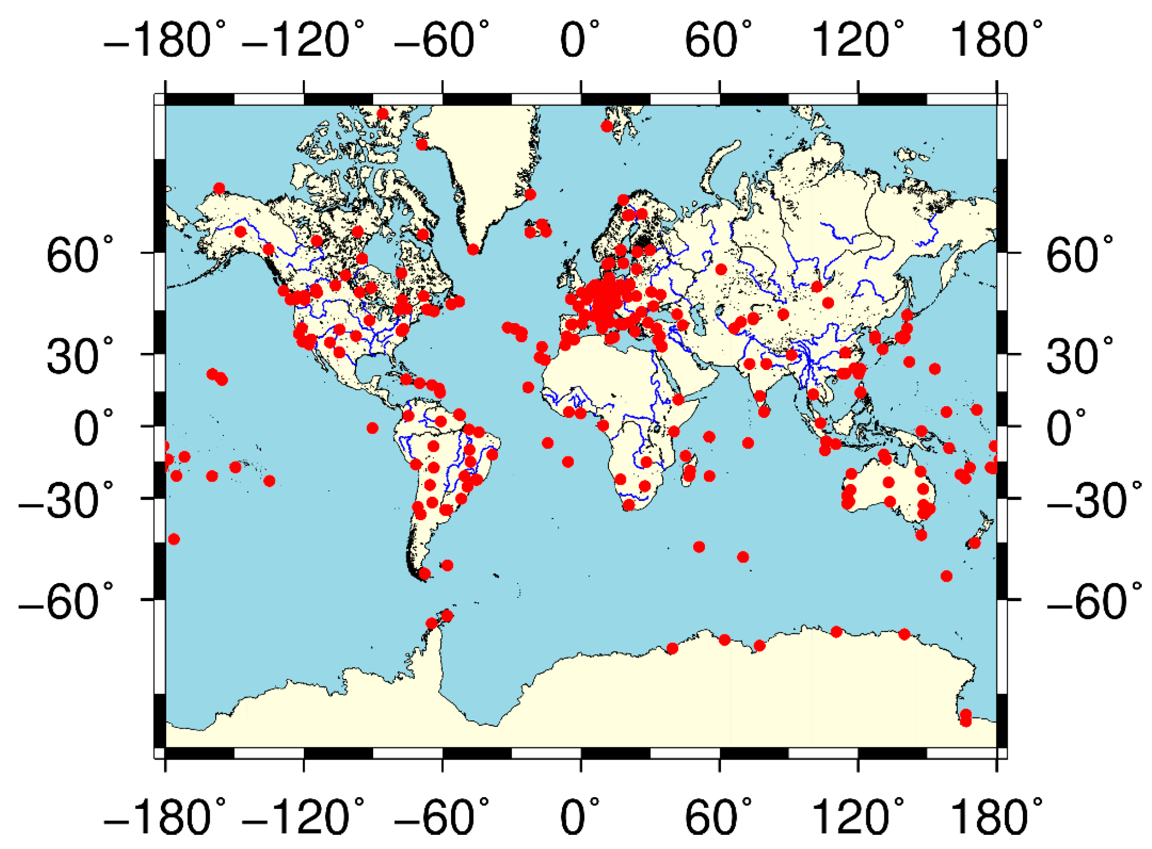
3. Experimental Data and Parameter Estimation Strategy

Usually, a global or a regional dense network is necessary for the multi-GNSS biases estimation, and, hence, the observables from 340 multi-GNSS experiment campaign (MGEX) network tracking stations (Figure 3) [34], recorded from DOY 290, 2021 to DOY 310, 2021, are utilized. All those stations can track GPS and Galileo multiple frequencies, and more than 170 stations and 160 stations can observe BDS-2, BDS-3, and GLONASS multi-frequency signals. Besides, to avoid the additional GLONASS IFBs among different types of receivers, about 80 stations equipped with SEPT POLARX5 receivers are selected to estimate GLONASS UPDs.
The IFCBs, OSBs, and PPP estimation strategies are summarized in Table 1. The elevation mask is set as 7°, and the triple-frequency uncombined observables with an interval of 30 s are processed. Clock slip is detected using the difference between epoch and cycle slip is detected with the triple-frequency TurboEdit method [35] and we adopt the GBM post precise products and igs14 antenna model. The zenith hydrostatic delay (ZHD) is calibrated with the Saastamoinen model [36] and the GPT3 meteorological parameter [37], and the tropospheric zenith wet delay (ZWD) is corrected using the Askne and Nordius model [38] and the GPT3 meteorological parameter [37], with corresponding mapping function VMF3 [37]. The residual zenith wet delay, the ionospheric delay, and ISB are estimated as random walk, and ambiguity parameters and receiver clock correction are modeled as constant and white noise, respectively. If cycle slips happen, the ambiguity parameters will be initialized with a large variance. To further reduce the estimated parameters, the station coordinates are fixed to the reference values published by the IGS daily solution independent exchange format (SINEX) files.
Table 2 further lists satellite systems, frequencies used to estimate IFCBs and phase OSBs, and codes used to estimate code OSBs in the experiment.
Table 3 describes the experimental platform used in the experiment. The GNSS data parallel processing software GNSSer [21] was utilized to obtain the IFCB and OSB products. Since GNSSer was developed using C#, TPL matches C# perfectly, simplifying the process of adding parallelism and concurrency to GNSS data processing. The software has a user-friendly interface and a high degree of automation, i.e., the ability to automatically download precise products from the IGS corresponding to the pending tasks.

4. Experimental Results and Discussions

In this section, multi-system IFCBs are estimated and investigated first. Then, the code and phase OSB products are analyzed and discussed. Finally, the speed-up effect of parallel computing is evaluated.

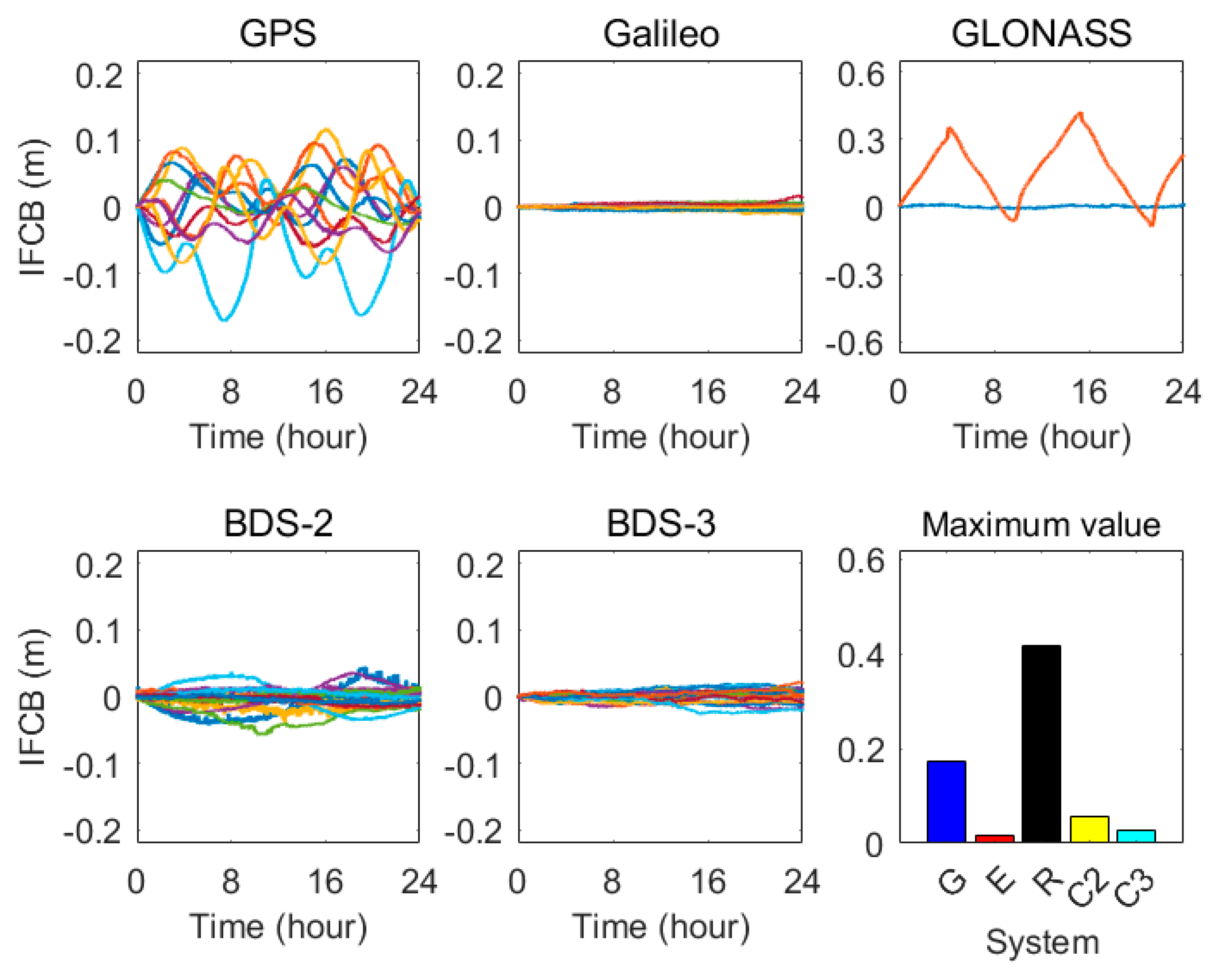
4.1. Characteristic of Multi-GNSS IFCBs

IFCB is an indispensable prerequisite for multi-frequency PPP and UPDs estimation. Figure 4 shows the multi-GNSS IFCB series and maximum values on DOY 290, 2021. It can be found that the IFCBs of different system present different variation amplitude.
(1)
For the 12 GPS Block IIF satellites, the IFCB errors reach more than 0.1 m, which is nonnegligible and must be carefully calibrated when using the triple-frequency observations, and the phenomenon has been first founded by Montenbruck et al. [15]. The newly launched Block III satellite has a small magnitude of IFCB errors;
(2)
With the IFCB amplitude of more than 5 cm, the same phenomenon has been occurred on some BDS-2 satellites, and this has been reported by Pan et al. [39];
(3)
Among the GLONASS constellation, in addition to transmitting traditional FDMA signals, a code division multiple access (CDMA) signal at 1202.025 Hz can be broadcast by 4 M+ satellites and 2 K1 satellites. During the selected period, the ground stations can track the G3 signal from K1 satellite R09 and M+ satellite R21. It can be seen that the variation of IFCB errors for R09 is tiny and stable, while that of R21 is fluctuating, and periodical variation has also been observed [40];
(4)
Currently, the BDS-3 satellites broadcast service on six frequencies, namely, B1C, B1I, B2a, B2b, B2a+b, and B3I. The IFCB errors of BDS-3 satellites are relatively small and can be neglected during the precise observation data handling, which has been pointed by Pan et al. [39];
(5)
The Galileo satellite shows the smallest IFCB errors among these four GNSS constellations. The possible reasons can be attributed to the better manufacturing process and high-performance satellite atomic clock.
The comparison reveals that the IFCB errors of Galileo satellites are exceptionally marginal, while GLONASS-M+ satellite R21 shows the largest IFCB errors of larger than 0.3 m. The possible reason may be attributable to that GLONASS M+ satellite transmits G3 signal from a different antenna, and the antenna phase center offset between GLONASS G1/G2 antenna and G3 antenna is more than 0.5 m on the y axis of satellite body coordinate [41], and, thus, the estimated IFCBs absorb this inconsistency. Since GLONASS K1 satellite R26 also presents this inconsistency, its IFCB errors may also be very large.
Furthermore, Figure 5 shows the multi-GNSS IFCB series and maximum values from DOY 290, 2021 to DOY 310, 2021. Through statistics, with an averaged root mean square (RMS) of 4.29 cm and a maximum value of 17.20 cm, the IFCB errors of GPS Block IIF satellites present significant and periodical fluctuation. The maximum IFCB errors of BDS-2, BDS-3, and Galileo satellites are 5.83, 4.07, and 2.32 cm, respectively, and the RMS values of these three systems are 1.09, 0.74, and 0.33 cm, respectively, during the selected period. Additionally, with periodical variation, the IFCB amplitude and RMS of GLONASS M+ satellite R21 are 61.00 cm and 11.46 cm, respectively, which are the biggest among those GNSS constellations.
Through the aforementioned analysis and discussions, it can be concluded that the IFCBs of GPS Block IIF and GLONASS-M+ satellites should be corrected in advance, while those of other systems can be neglected due to their small magnitude. Additionally, the periodical variation characteristic makes it possible to model IFCB errors and obtain high-accuracy forecast values.

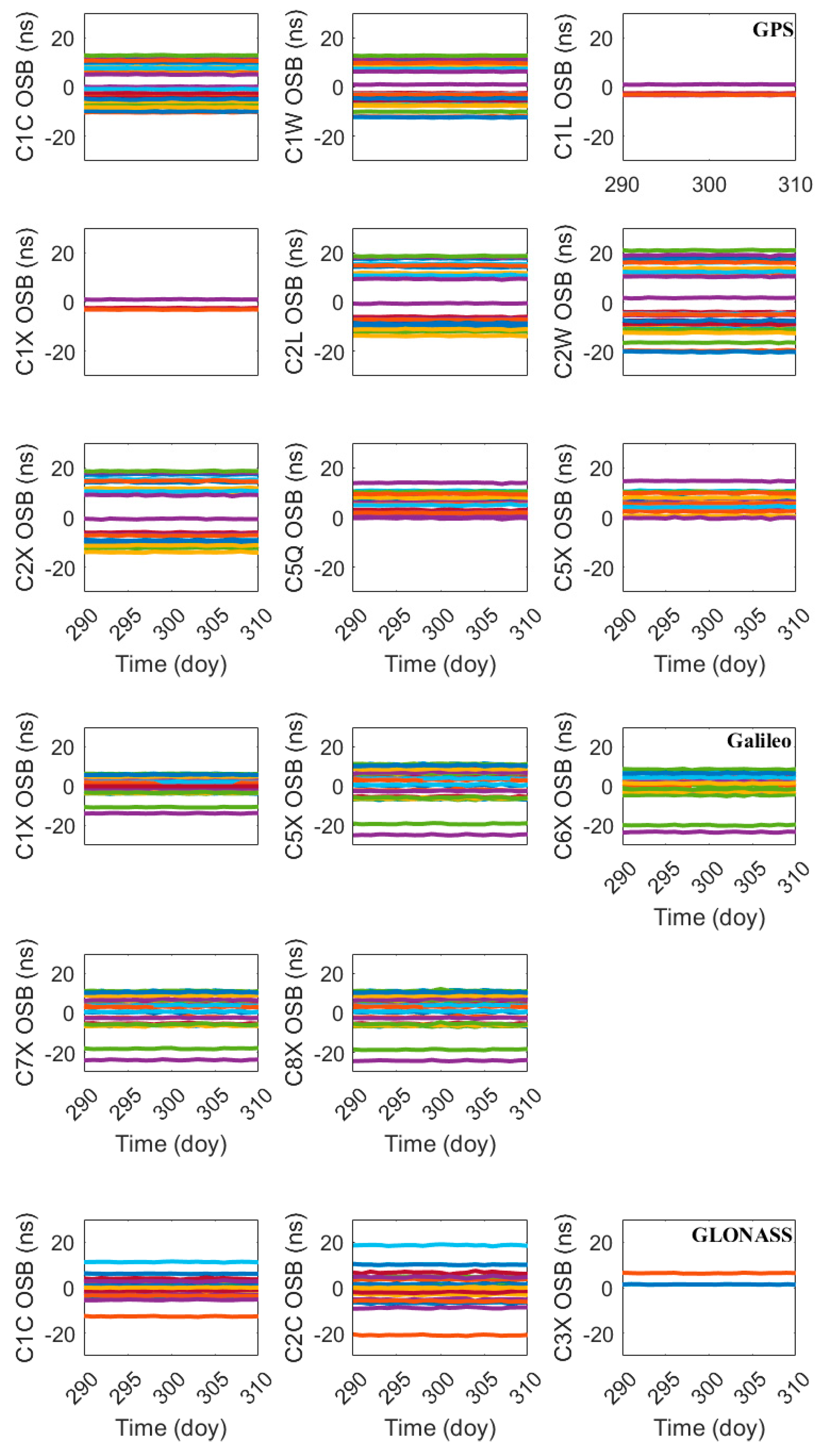
4.2. Characteristic of Code OSBs

Figure 6 shows the multi-GNSS code OSB series form DOY 290, 2021 to DOY 310, 2021. Table 4 further gives the statistical STDs. It can be concluded that:
(1)
Among those systems, the satellite code OSBs of GPS are the most stable, and their average STD is less than 0.10 ns;
(2)
Currently, all the 26 Galileo satellites are able to provide five-frequency signals. It can be seen that all these code OSBs are generally stable and, owing to the special Alt-BOC modulation, the code OSBs on E5a (C5X), E5b (C7X), and E5ab (C8X) are highly consistent, which has also been discussed in Li et al. [14];
(3)
For GLONASS satellites, the STDs of C1C, C2C, and C3X OSBs are 0.13, 0.21, 0.11 ns, respectively. The code OSB on the G3 CDMA signal shows slightly better stability than the other two FDMA frequencies;
(4)
The magnitudes of BDS-2 and BDS-3 code OSBs are approximately 100 and 200 ns, respectively, which are larger than other systems. The BDS3 code OSBs show slightly better stability than the BDS2 code OSBs.

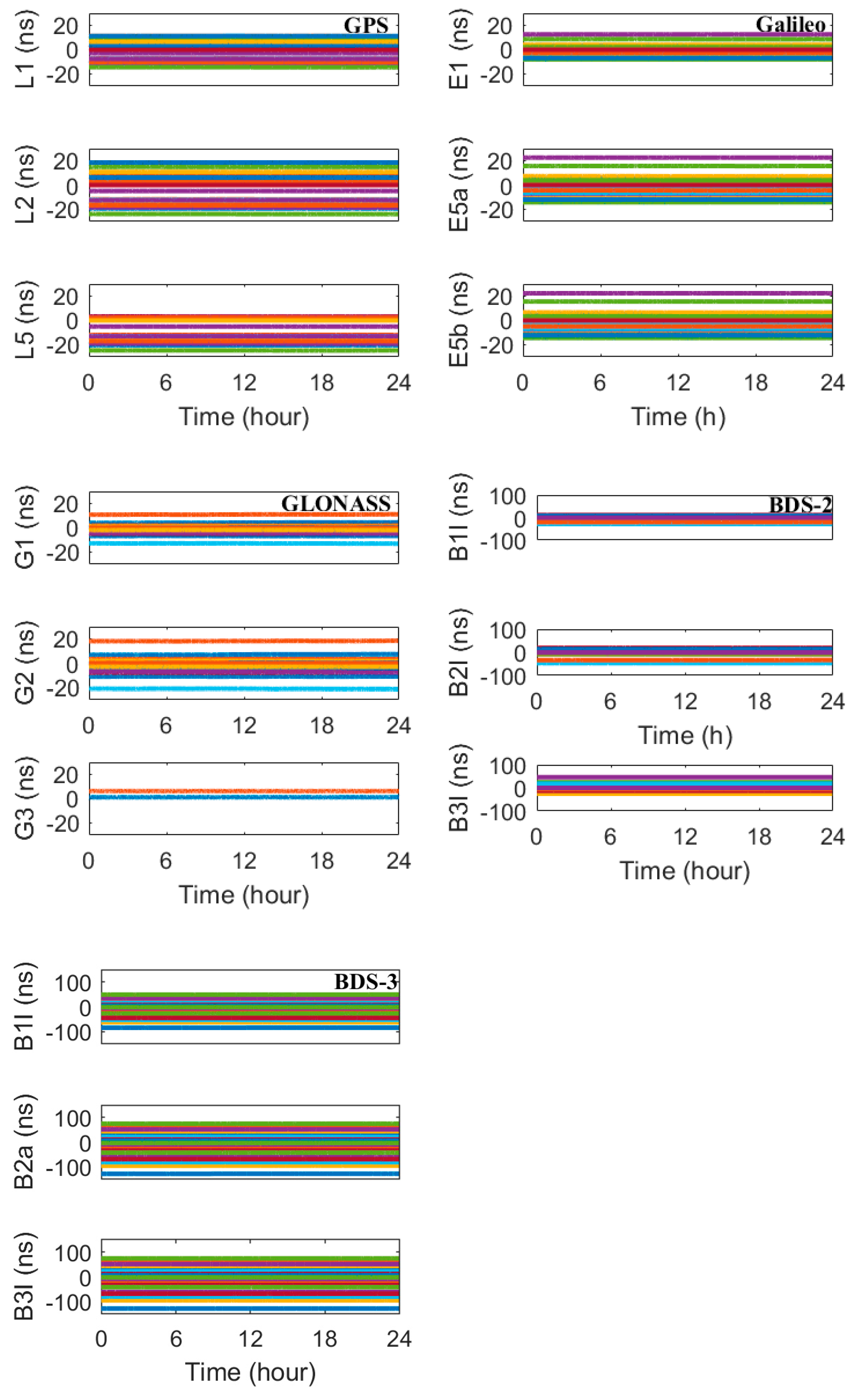
4.3. Characteristic of Phase OSBs

Figure 7 shows the multi-GNSS phase OSB series on DOY 290, 2021. The interval is 30 s. Figure 8 further gives the statistical result of STDs from DOY 290, 2021 to DOY 310, 2021. It can be concluded that:
(1)
With an average STD less than 0.05 ns, the phase OSBs of GPS, Galileo, BDS-2, and BDS-3 satellites are very stable, wherein Galileo shows the optimal result. The possible reason may also be attributable to the high-performance atomic clocks that Galileo utilized;
(2)
For GLONASS satellite, the STDs of G1, G2, and G3 phase OSBs are 0.08, 0.11, and 0.09 ns, respectively, which are slightly larger than those of other systems. The possible reason could be due to the GLONASS IFBs, although the same receiver type is selected, there is slight difference in the receiver version number, which will bring biases for phase OSBs estimation.
Hence, considering the stability of phase OSBs, the phase OSB products could be published with a longer sampling interval. With the estimated IFCBs and OSBs, users can directly correct the original pseudorange and phase observations of multiple systems and multiple frequencies, allowing for convenient data processing and ambiguity fixation.

4.4. Evaluation of Parallel Acceleration Ratio

Five parallel computing schemes involving a different number of physical cores, along with the traditional serial computing, were carried out. The time spent on the experiment was averaged through the repeat of three times.
Usually, using a serial computing method, the undifferenced and uncombined PPP of each station takes 28 s, and about 8 min, 260 min, and 12 min for IFCBs estimation, code OSBs estimation and ionospheric modeling, and phase OSBs estimation, respectively. It can be concluded that most of the time is spent on PPP and global ionospheric modeling, which can be accelerated using multi-station parallel computing, multi-satellite parallel computing, and matrix parallel operation.
Table 5 gives the computation time and acceleration rate using different scheme. The acceleration rates using four, eight, sixteen, and thirty-two cores are 3.10, 5.53, 9.66, and 17.04 times, respectively, compared to the serial computing scheme using a single core. Using a quad-core platform, the time spent on PPP per station, IFCBs estimation, code OSBs estimation, and phase estimation are 10 s, 3 min, 80 min, and 4 min, respectively. As the quantity of input cores increases, the time spent on parallel computing overheads involving synchronization, communication, and coordination increases quite a lot, and the improvement of parallel computing efficiency is reduced and limited [17,18,19]. More threads tend to compete for CPU resources, thus reducing the computational efficiency. Moreover, the established file locks in Figure 1 during IFCBs and OSBs estimation, which force the parallel program to serially execute, also decrease the speed-up ratio. However, with more invested cores, the efficiency for IFCBs and OSBs publication is greatly improved, and the time for releasing those products to GNSS users with multiple systems and multiple frequencies can be substantially reduced.

5. Discussions

To achieve optimal fusion of multi-frequency GNSS data, the biases need to be finely considered and modeled. In this contribution, IFCBs and OSBs are estimated as two types of parameters. By absorbing IFCBs, Su et al. [42] proposed a more flexible and unified correction product, and it is the phase time-varying OSBs. This kind of product deserves our further research.
Besides, the accuracy of the estimated IFCBs and OSBs can be validated in three aspects. The first is the comparison with the OSB products published by other organizations. By converting the datum, approximately 95% of the residuals for the code OSBs are less than 0.2 ns, indicating that our products are in good agreement with CAS, but, for the phase OSBs, since they absorb various errors, i.e., parameter and model settings of different software, an alternative approach is the performance of PPP ambiguity fixing of multi-system and multi-frequency [14,43,44,45]. Using the triple-frequency observations from the European permanent network and Henan providence, China, the average static hourly positioning accuracy of 4.0 and 7.0 mm can be achieved in the horizontal and vertical components, respectively. It costs approximately 5.0 and 6.0 min to realize the coordinate convergence and the first time to fix ambiguity. The last validation method is to use the massive observations from the large-scale GNSS network and convert the observations into carrier ranges [46], then huge GNSS network processing using the carrier range is conducted. Utilizing the approximately 250 stations from the Crustal Movement Observation Network of China (CMONOC), and the parallel computing method of the huge GNSS network being extended to triple-frequency as according to Li et al. [47], the daily static coordinate accuracy of better than 3.0 and 5.0 mm is realized in the horizontal and vertical components, respectively, and the ambiguity fixing rate reaches more than 92.0%. Since the emphasis of this contribution is the parallel estimation of IFCBs and OSBs, the results of the aforementioned two validations are not provided in detail.

6. Conclusions

To accelerate the computation speed and reduce the time consumption of IFCBs and OSBs, this paper proposed an efficient parallel computation method using TPL. The key findings are summarized as:
  • Among multiple systems, the IFCBs of GPS Block IIF and GLONASS M+ satellites present periodical variation, and their amplitudes are nonnegligible, wherein the GLONASS M+ satellite R21 shows the largest IFCB of more than 0.60 m;
  • For all the four systems, the daily code OSBs present high stability with average STDs smaller than 0.20 ns, among which GPS presents the smallest STD of 0.10 ns;
  • The phase OSBs show the stability of better than 0.10 ns, wherein the Galileo satellites presents the optimal performance of 0.01 ns;
  • Under a multicore platform, the acceleration effect is significant, which can significantly shorten the computation time for IFCBs and OSBs estimation.
However, the proposed parallel computing method can be further extended to multiple computers with different configurations. The message passing interface (MPI) and Hadoop MapReduce can be applied. Parallel computing based on graphics processing units (GPUs) has advantages over multi-core CPUs, which is the next step in our research. The application of those absolute biases will also be investigated further.

Author Contributions

L.L. and Z.Y. proposed the parallel computing scheme, L.L. and Z.J. wrote and tested the parallel program, and L.L. and X.L. prepared the experimental data and platform, and carried out the experiments. All authors participated in the result analysis and manuscript writing. All authors have read and agreed to the published version of the manuscript.

Funding

This work was funded by the National Natural Science Foundation of China (grant nos. 42104033) and the excellent Post-Doctoral Program of Jiangsu Province (grant nos. 2022ZB166).

Data Availability Statement

The experimental data used in the manuscript have been downloaded from the IGS analysis center, and the data download websites are ftp://igs.ign.fr/pub/igs/data/campaign/mgex/daily/rinex3 and ftp://igs-ftp.bkg.bund.de/IGS/obs, respectively, accessed on 1 October 2022.

Acknowledgments

The authors thank IGS for providing GNSS multi-frequency observation data and precise satellite products.

Conflicts of Interest

The authors declare no conflict of interest.

References

  1. Teunissen, P.J.G.; Montenbruck, O. Springer Handbook of Global Navigation Satellite Systems; Springer: Cham, Switzerland, 2017; pp. 3–22. [Google Scholar]
  2. Hein, G.W. Status, perspectives and trends of satellite navigation. Satell. Navig. 2020, 1, 22. [Google Scholar] [CrossRef]
  3. Montenbruck, O.; Hauschild, A.; Steigenberger, P. Differential code bias estimation using multi-GNSS observations and global ionosphere maps. Navigation 2014, 61, 191–201. [Google Scholar] [CrossRef]
  4. Zhang, B.; Teunissen, P.J.G.; Yuan, Y.; Zhang, X.; Li, M. A modified carrier-to-code leveling method for retrieving ionospheric observables and detecting short-term temporal variability of receiver differential code biases. J. Geod. 2019, 93, 19–28. [Google Scholar] [CrossRef] [Green Version]
  5. Ge, M.; Gendt, G.; Rothacher, m.; Shi, C.; Liu, J. Resolution of GPS carrier-phase ambiguities in precise point positioning (PPP) with daily observations. GPS Solut. 2008, 82, 389–399. [Google Scholar]
  6. Zhang, B.; Teunissen, P.J.G.; Yuan, Y. On the short-term temporal variations of GNSS receiver differential phase biases. J. Geod. 2017, 91, 563–572. [Google Scholar] [CrossRef] [Green Version]
  7. Deng, Y.; Guo, F.; Ren, X.; Ma, F.; Zhang, X. Estimation and analysis of multi-GNSS observable-specific code biases. GPS Solut. 2021, 25, 100. [Google Scholar] [CrossRef]
  8. Wang, N.; Li, Z.; Duan, B.; Hugentobler, U.; Wang, L. GPS and GLONASS observable-specific code bias estimation: Comparison of solutions from the IGS and MGEX networks. J. Geod. 2020, 94, 74. [Google Scholar] [CrossRef]
  9. Li, M.; Yuan, Y. Estimation and analysis of the observable-specific code biases estimated using multi-GNSS observations and global ionospheric maps. Remote Sens. 2021, 13, 3096. [Google Scholar] [CrossRef]
  10. Schaer, S. SINEX BIAS-solution (software/technique) INdependent EXchange format for GNSS biases version 1.00. In Proceedings of the IGS Workshop on GNSS Biases, Bern, Switzerland, 8–12 February 2016; pp. 1–37. [Google Scholar]
  11. Schaer, S.; Villiger, A.; Arnold, D.; Dach, R.; Prange, L.; Jäggi, A. The CODE ambiguity-fixed clock and phase bias analysis products: Generation, properties, and performance. J. Geod. 2021, 95, 81. [Google Scholar] [CrossRef]
  12. Liu, T.; Zhang, B. Estimation of code observation-specific biases (OSBs) for the modernized multi-frequency and multi-GNSS signals: An undifferenced and uncombined approach. J. Geod. 2021, 95, 97. [Google Scholar] [CrossRef]
  13. Geng, J.; Zhang, Q.; Li, G.; Liu, J.; Liu, D. Observable-specific phase biases of Wuhan multi-GNSS experiment analysis center’s rapid satellite products. Satell. Navig. 2022, 3, 23. [Google Scholar] [CrossRef]
  14. Li, X.; Li, X.; Jiang, Z.; Xia, C.; Shen, Z.; Wu, J. A unified model of GNSS phase/code bias calibration for PPP ambiguity resolution with GPS, BDS, Galileo and GLONASS multi-frequency observations. GPS Solut. 2022, 26, 84. [Google Scholar] [CrossRef]
  15. Montenbruck, O.; Hugentobler, U.; Dach, R.; Steigenberger, P.; Hauschild, A. Apparent clock variations of the Block IIF-1 (SVN62) GPS satellite. GPS Solut. 2012, 16, 303–313. [Google Scholar] [CrossRef]
  16. Boomkamp, H. Global GPS reference frame solutions of unlimited size. Adv. Space Res. 2010, 46, 136–143. [Google Scholar] [CrossRef]
  17. Kuang, K.; Zhang, S.; Li, J. Real-time GPS satellite orbit and clock estimation based on OpenMP. Adv. Space Res. 2019, 63, 2378–2386. [Google Scholar] [CrossRef]
  18. Li, L.; Lu, Z.; Chen, Z.; Cui, Y.; Kuang, Y.; Wang, F. Parallel computation of regional CORS network corrections based on ionospheric-free PPP. GPS Solut. 2019, 23, 70. [Google Scholar] [CrossRef]
  19. Chen, X.; Ge, M.; Hugentobler, U.; Schuh, H. A new parallel algorithm for improving the computational efficiency of multi-GNSS precise orbit determination. GPS Solut. 2022, 26, 83. [Google Scholar] [CrossRef]
  20. Bertiger, W.; Bar-Sever, Y.; Dorsey, A.; Haines, B.; Harvey, N.; Hemberger, D.; Heflin, M.; Lu, W.; Miller, M.W.; Moore, A.; et al. GipsyX/RTGx, a new tool set for space geodetic operations and research. Adv. Space Res. 2020, 66, 469–489. [Google Scholar] [CrossRef]
  21. Li, L.; Lu, Z.; Chen, Z.; Cui, Y.; Sun, D.; Wang, Y.; Kuang, Y.; Wang, F. GNSSer: Objected-oriented and design pattern-based software for GNSS data parallel processing. J. Spat. Sci. 2021, 66, 27–47. [Google Scholar] [CrossRef]
  22. Li, H.; Zhou, X.; Wu, B.; Wang, J. Estimation of the inter-frequency clock bias for the satellites of PRN25 and PRN01. Sci. China Phys. Mech. Astron. 2012, 55, 2186–2193. [Google Scholar] [CrossRef]
  23. Fan, L.; Shi, C.; Li, M.; Wang, C.; Zheng, F.; Jing, G.; Zhang, J. GPS satellite inter-frequency clock bias estimation using triple-frequency raw observations. J. Geod. 2019, 93, 2465–2479. [Google Scholar] [CrossRef]
  24. Li, L.; Lu, Z.; Cui, Y.; Wang, Y.; Huang, X. Parallel resolution of large-scale GNSS network un-difference ambiguity. Adv. Space Res. 2017, 60, 2637–2647. [Google Scholar] [CrossRef]
  25. Zhang, F.; Chai, H.; Wang, M.; Bai, T.; Li, L.; Guo, W.; Du, Z. Considering inter-frequency clock bias for GLONASS FDMA + CDMA precise point positioning. GPS Solut. 2023, 27, 10. [Google Scholar] [CrossRef]
  26. Pan, L.; Zhang, X.; Li, X.; Liu, J.; Li, X. Characteristics of inter-frequency clock bias for Block IIF satellites and its effect on triple-frequency GPS precise point positioning. GPS Solut. 2017, 21, 811–822. [Google Scholar] [CrossRef]
  27. Cui, Y.; Lu, Z.; Chen, Z.; Wang, Y.; Lu, H. Research of parallel data processing for GNSS network adjustment under multi-core environment. Acta Geod. Cartogr. Sin. 2013, 42, 661–667. [Google Scholar]
  28. Montenbruck, O.; Hauschild, A. Code biases in multi-GNSS point positioning. In Proceedings of the International Technical Meeting of The Institute of Navigation (ION ITM), San Diego, CA, USA, 27–29 January 2013; pp. 616–628. [Google Scholar]
  29. Dong, D.; Bock, Y. Global Positioning System network analysis with phase ambiguity resolution applied to crustal deformation studies in California. J. Geophys. Res. 1989, 94, 3949–3966. [Google Scholar] [CrossRef]
  30. Li, L.; Cui, Y.; Wang, Y.; Lu, Z. Improvement of narrow-lane fractional cycle bias estimation and analysis of its time-varying Property. Acta Geod. Cartogr. Sin. 2017, 46, 34–43. [Google Scholar]
  31. Wanninger, L.; Beer, S. BeiDou satellite-induced code pseudorange variations, diagnosis and therapy. GPS Solut. 2015, 19, 639–648. [Google Scholar] [CrossRef] [Green Version]
  32. Beer, S.; Wanninger, L.; Hesselbarth, A. Estimation of absolute GNSS satellite antenna group delay variations based on those of absolute receiver antenna group delays. GPS Solut. 2021, 25, 110. [Google Scholar] [CrossRef]
  33. Zhou, F.; Dong, D.; Ge, M.; Li, P.; Wickert, J.; Schuh, H. Simultaneous estimation of GLONASS pseudorange inter-frequency biases in precise point positioning using undifferenced and uncombined observations. GPS Solut. 2018, 22, 19. [Google Scholar] [CrossRef]
  34. Montenbruck, O.; Steigenberger, P.; Prange, L.; Deng, Z.; Zhao, Q.; Perosanz, F.; Schmid, R. The Multi-GNSS experiment (MGEX) of the international GNSS service (IGS)-achievements, prospects and challenges. Adv. Space Res. 2017, 59, 1671–1697. [Google Scholar] [CrossRef]
  35. Huang, L.; Zhai, G.; Ouyang, Y.; Lu, X.; Wu, T.; Deng, K. Triple-frequency TurboEdit cycle-slip processing method of weakening ionospheric activity. Acta Geod. Cartogr. Sin. 2015, 44, 840–847. [Google Scholar]
  36. Saastamoinen, J. Atmospheric correction for the troposphere and stratosphere in radio ranging of satellites. The use of artificial satellites for geodesy. Geophys. Monogr. Ser. 1972, 15, 247–251. [Google Scholar]
  37. Landskron, D.; Böhm, J. VMF3/GPT3: Refined discrete and empirical troposphere mapping functions. J. Geod. 2018, 92, 349–360. [Google Scholar] [CrossRef]
  38. Askne, J.; Nordius, H. Estimation of tropospheric delay for microwaves from surface weather data. Radio Sci. 1987, 22, 379–386. [Google Scholar] [CrossRef]
  39. Pan, L.; Li, X.; Zhang, X.; Li, X.; Lu, C.; Zhao, Q.; Liu, J. Considering inter-frequency clock bias for bds triple- frequency precise point positioning. Remote Sens. 2017, 9, 734. [Google Scholar] [CrossRef] [Green Version]
  40. Zhang, F.; Chai, H.; Li, L.; Wang, M.; Feng, X.; Du, Z. Understanding the characteristic of GLONASS inter-frequency clock bias using both FDMA and CDMA signals. GPS Solut. 2022, 26, 63. [Google Scholar] [CrossRef]
  41. Montenbruck, O.; Schmid, R.; Mercier, F.; Steigenberger, P.; Noll, C.; Fatkuline, R.; Koguref, S.; Ganeshan, A.S. GNSS satellite geometry and attitude models. Adv. Space Res. 2015, 56, 1015–1029. [Google Scholar] [CrossRef] [Green Version]
  42. Su, K.; Jin, S.; Jiao, G. GNSS carrier phase time-variant observable-specific signal bias (OSB) handling: An absolute bias perspective in multi-frequency PPP. GPS Solut. 2022, 26, 71. [Google Scholar] [CrossRef]
  43. Geng, J.; Guo, J.; Meng, X.; Gao, K. Speeding up PPP ambiguity resolution using triple-frequency GPS/BeiDou/Galileo/QZSS data. J. Geod. 2020, 94, 6. [Google Scholar] [CrossRef] [Green Version]
  44. Du, S.; Shu, B.; Xie, W.; Huang, G.; Ge, Y.; Li, P. Evaluation of Real-time Precise Point Positioning with Ambiguity Resolution Based on Multi-GNSS OSB Products from CNES. Remote Sens. 2022, 14, 4970. [Google Scholar] [CrossRef]
  45. Li, B.; Mi, J.; Zhu, H.; Gu, S.; Xu, Y.; Wang, H.; Yang, L.; Chen, Y.; Pang, Y. BDS-3/GPS/Galileo OSB Estimation and PPP-AR Positioning Analysis of Different Positioning Models. Remote Sens. 2022, 14, 4207. [Google Scholar] [CrossRef]
  46. Chen, H.; Jiang, W.; Ge, M.; Wickert, J.; Schuh, H. An enhanced strategy for GNSS data processing of massive networks. J. Geod. 2014, 88, 857–867. [Google Scholar] [CrossRef]
  47. Li, L.; Lu, Z.; Li, J.; Kuang, Y.; Wang, F. Parallel resolution of large GNSS networks using carrier ranges. Adv. Space Res. 2020, 66, 2621–2628. [Google Scholar] [CrossRef]
Figure 1. The finer-grained parallel computing flowchart of undifferenced and uncombined PPP under a multicore platform. The symbol * represents the station name.
Remotesensing 15 01953 g001
Figure 2. The parallel estimation flowchart of IFCBs, code, and phase OSBs under a multicore platform. Three parallel computing methods involving inter-station, inter-satellite, and matrix operation are employed. The symbol * represents the station name.
Remotesensing 15 01953 g002
Figure 3. The distribution of 340 globally-distributed IGS MGEX tracking stations used in the experiment.
Remotesensing 15 01953 g003
Figure 4. The multi-GNSS IFCB series and maximum values on DOY 290, 2021. A different color line represents a different satellite. The orange and blue lines of GLONASS denote R21 and R09 satellites, respectively. The abbreviation G, E, R, C2, and C3 represents GPS, Galileo, GLONASS, BDS-2, and BDS-3, respectively.
Remotesensing 15 01953 g004
Figure 5. The multi-GNSS IFCB series and maximum values from DOY 290, 2021 to DOY 310, 2021. A different color line represents a different satellite.
Remotesensing 15 01953 g005
Figure 6. The multi-GNSS code OSB series from DOY 290, 2021 to DOY 310, 2021. A different color line represents a different satellite.
Remotesensing 15 01953 g006aRemotesensing 15 01953 g006b
Figure 7. The multi-GNSS phase OSB series on DOY 290, 2021. A different color line represents a different satellite.
Remotesensing 15 01953 g007
Figure 8. The average STDs of multi-GNSS phase OSBs from DOY 290, 2021 to DOY 310, 2021.
Remotesensing 15 01953 g008
Table 1. Processing strategies of the IFCBs and OSBs estimation, and multi-GNSS and multi-frequency PPP.
TypeProcessing Strategy
Sampling interval30 s
Elevation mask
Weight for observationsElevation-dependent weight
Satellite ephemeris and clock offsets filesGBM post precise products
Clock slip and cycle slipDifference between epochs and modified triple-frequency TurboEdit method
Antenna phase offsetigs14 antenna model
Tropospheric delayZHD is corrected using Saastamoinen + GPT3
ZWD is corrected using Askne and Nordius + GPT3
VMF3 mapping function
Ionospheric delay and ISBModeled as a random walk, with a power spectrum density of 1.7 × 10⁻⁴ and 1.7 × 10⁻⁷ m2/s, respectively
Tracking station
coordinates
Fixed to the IGS daily SINEX files
AmbiguityModeled as a constant without cycle slips, partial
ambiguity fixing, and the ratio value is set as 2.0
Receiver clock offsetWhite noise
Table 2. The selected frequencies and codes in the experiment.
SystemFrequencies Used to
Estimate IFCBs and Phase OSBs
Codes Used to Estimate Code OSBs
GPSL1, L2, L5C1C, C1W, C1L, C1X, C2L, C2W, C2X, C5Q, C5X
GalileoE1, E5a, E5bC1X, C5X, C6X, C7X, C8X
GLONASSG1, G2, G3C1C, C2C, C3X
BDS-2B1I, B2I, B3IC2I, C6I, C7I
BDS-3B1I, B2a, B3IC1P, C1X, C2I, C5P, C5X, C6I, C8X
Table 3. The experimental platform used in the experiment.
Experimental PlatformProcessorNumber of CoresMemory Size
Dell R750 workstation Intel Xeon gold processor 6314U, 3.40 GHz32 cores128 GB
Table 4. The STDs of multi-GNSS code OSBs during the selected period. (ns).
GPSGalileoGLONASSBDS-2BDS-3
STD0.100.210.170.230.21
Table 5. Computation time and acceleration rate using a different scheme.
Single CoreFour CoresEight CoresSixteen CoresThirty-Two Cores
Computation time (min)438141.3079.2045.3525.70
Acceleration rate---3.105.539.6617.04
Disclaimer/Publisher’s Note: The statements, opinions and data contained in all publications are solely those of the individual author(s) and contributor(s) and not of MDPI and/or the editor(s). MDPI and/or the editor(s) disclaim responsibility for any injury to people or property resulting from any ideas, methods, instructions or products referred to in the content.

