
Deep Machine Learning Based Possible Atmospheric and Ionospheric Precursors of the 2021 Mw 7.1 Japan Earthquake

 ,
,  , ,
, ,
Abstract
:1. Introduction
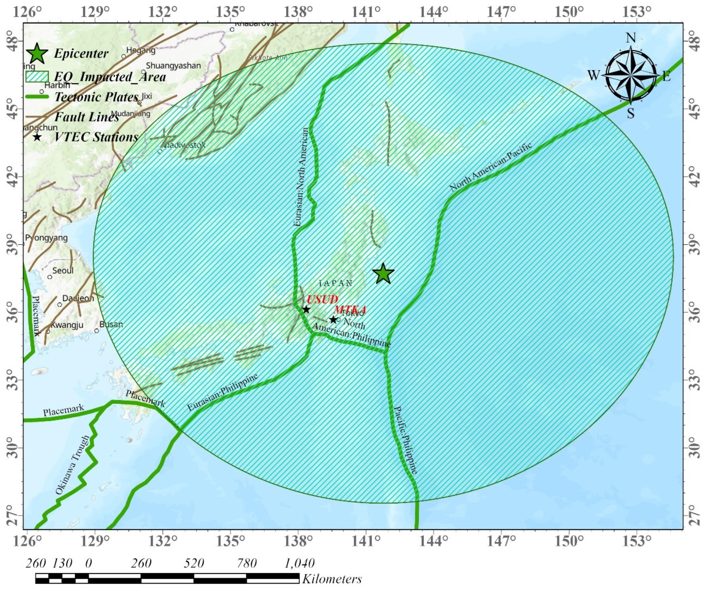
2. Study Area
3. Materials and Datasets
3.1. Outgoing Longwave Radiation
3.2. Relative Humidity
3.3. Air Temperature
3.4. Sea Surface Temperature
3.5. Total Electron Content
4. Methodology
4.1. Anomaly Detection Using Statistical Method
4.2. Anomaly Detection Using Wavelet Transformation
4.3. Anomaly Detection Using Artificial Neural Network (ANN)
4.4. Nonlinear Autoregressive Network with Exogenous Inputs (NARX)
4.5. Long Short-Term Memory (LSTM)
5. Results
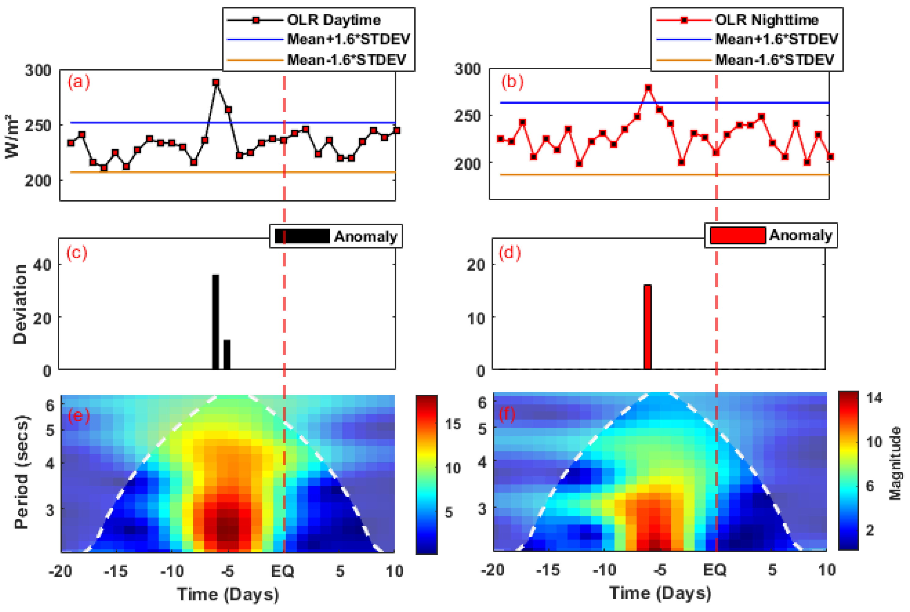
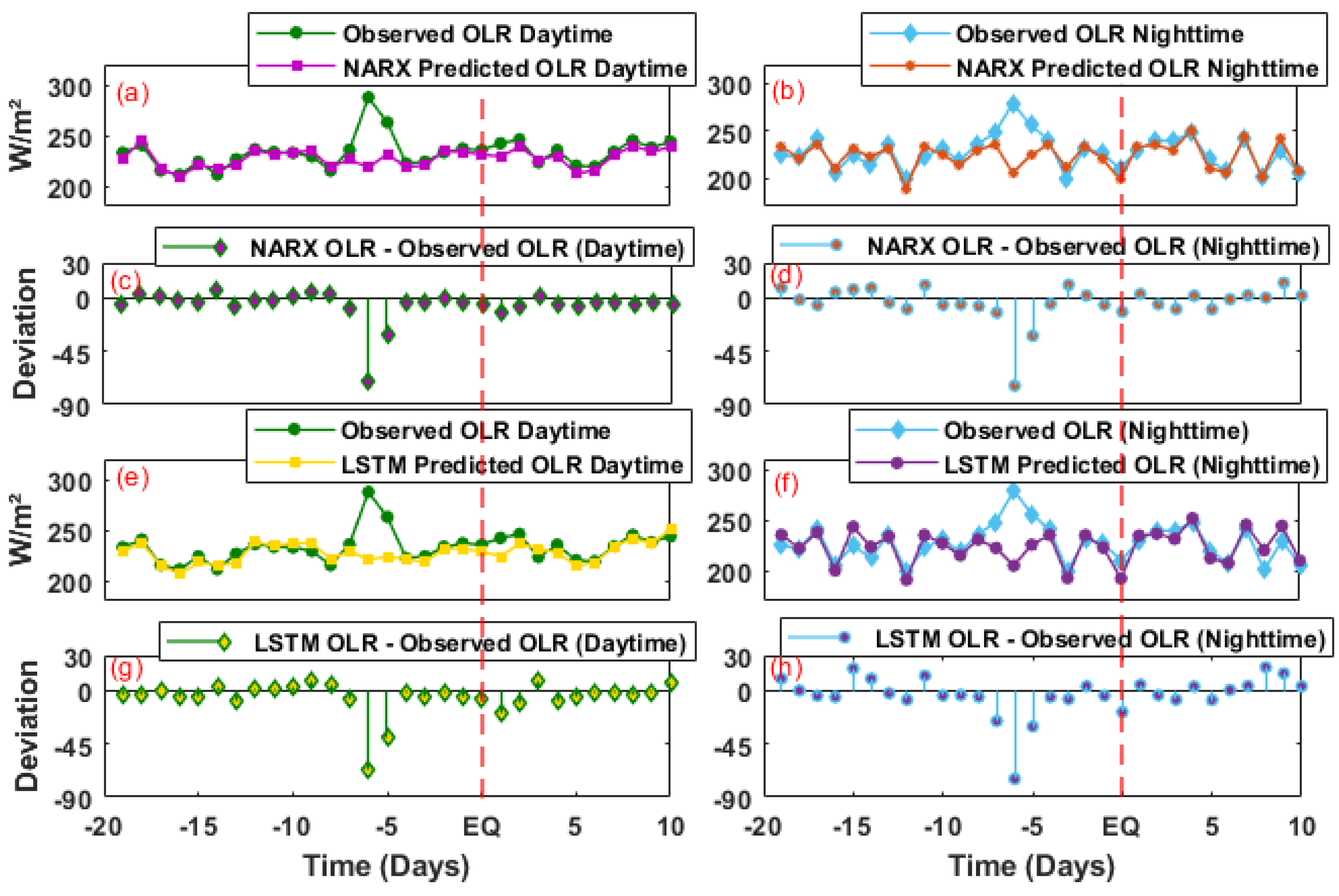
5.1. Outgoing Longwave Radiation
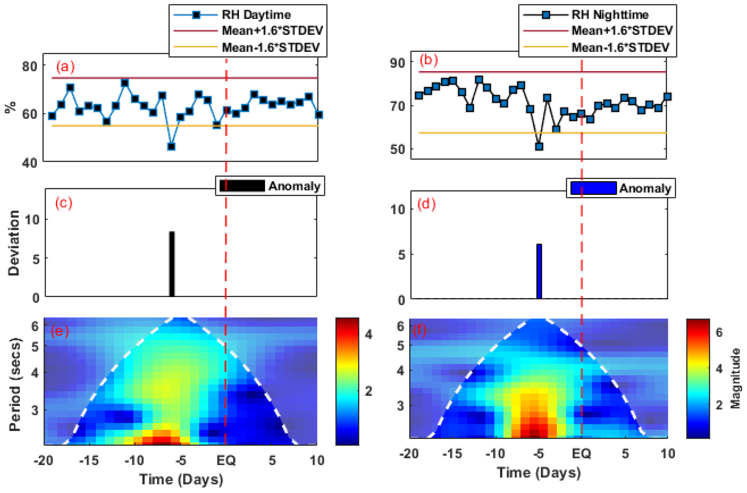
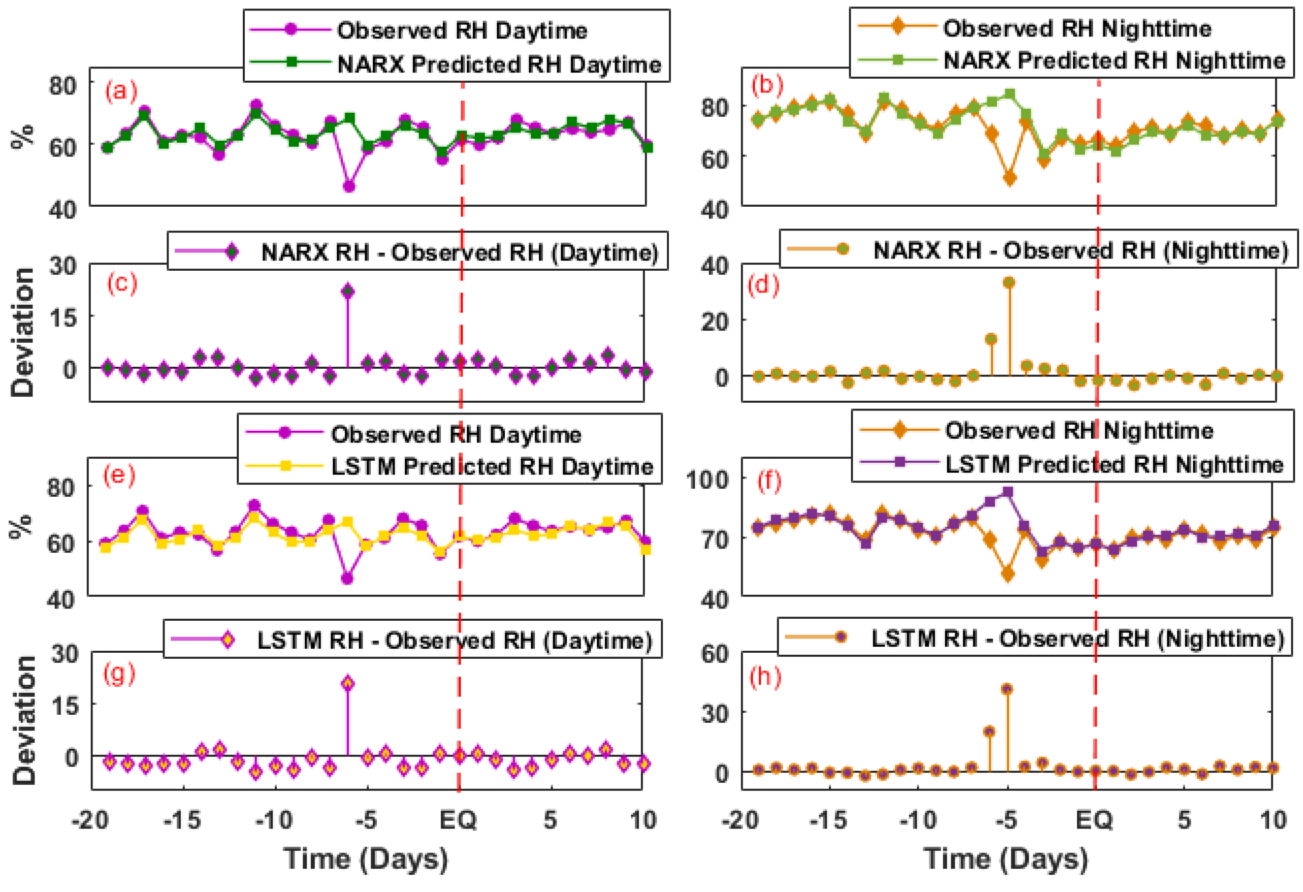
5.2. Relative Humidity
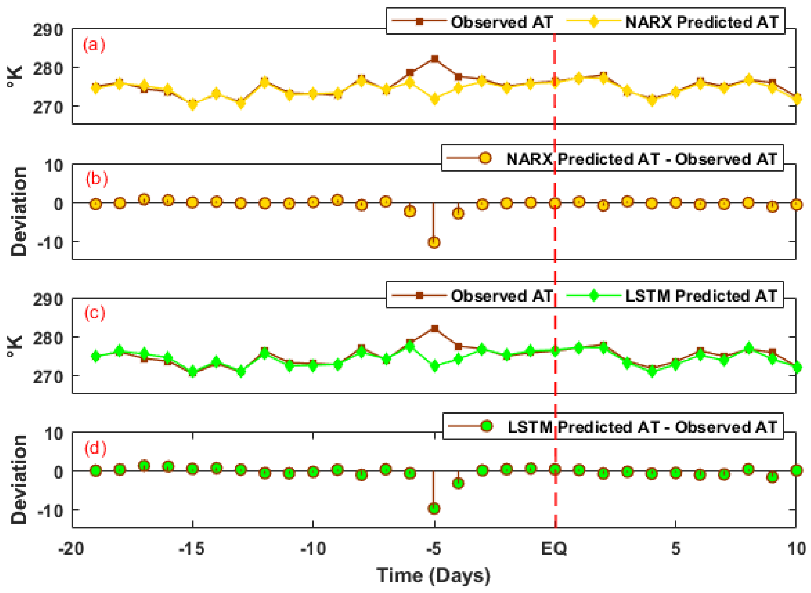
5.3. Air Temperature
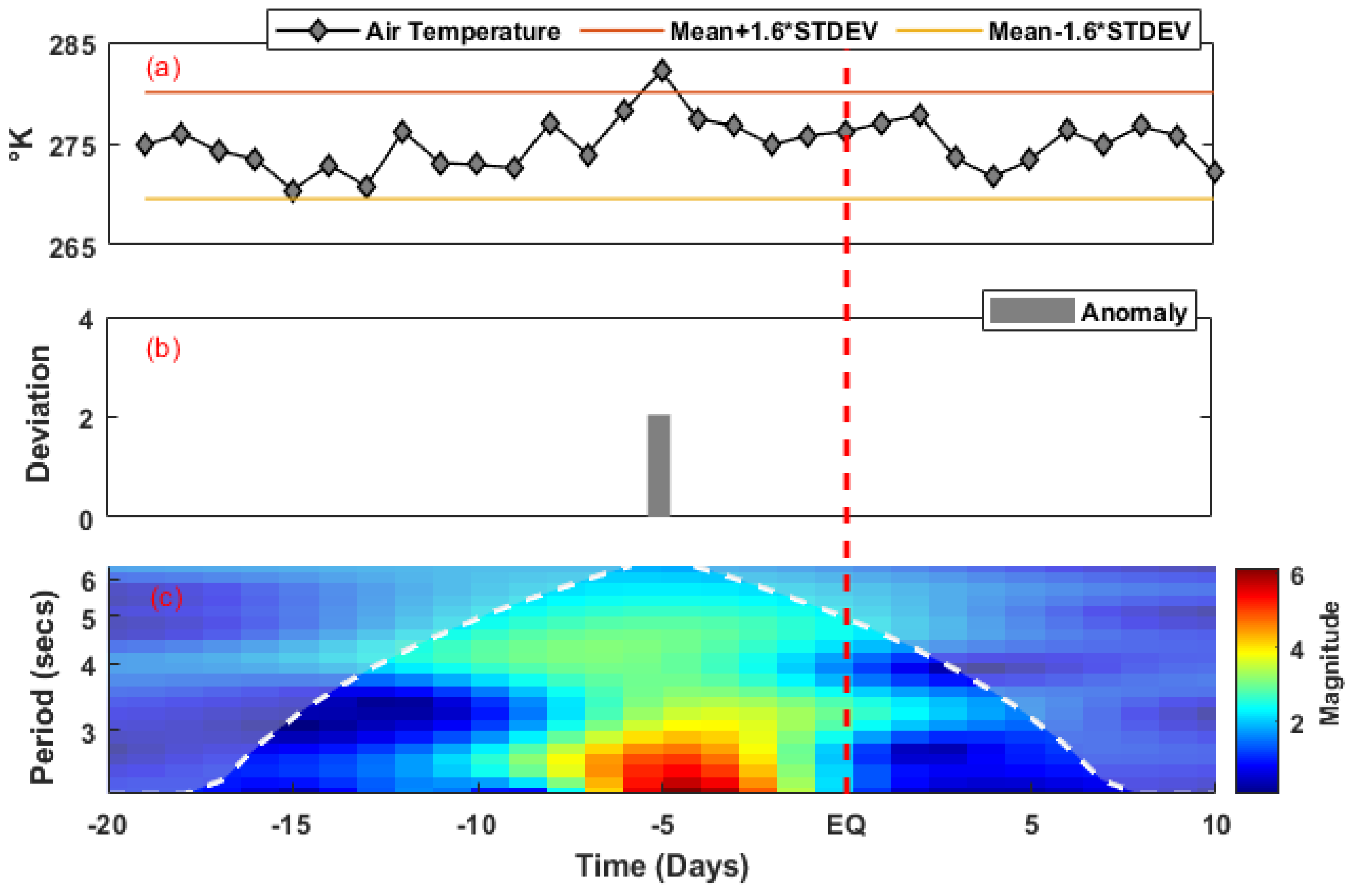
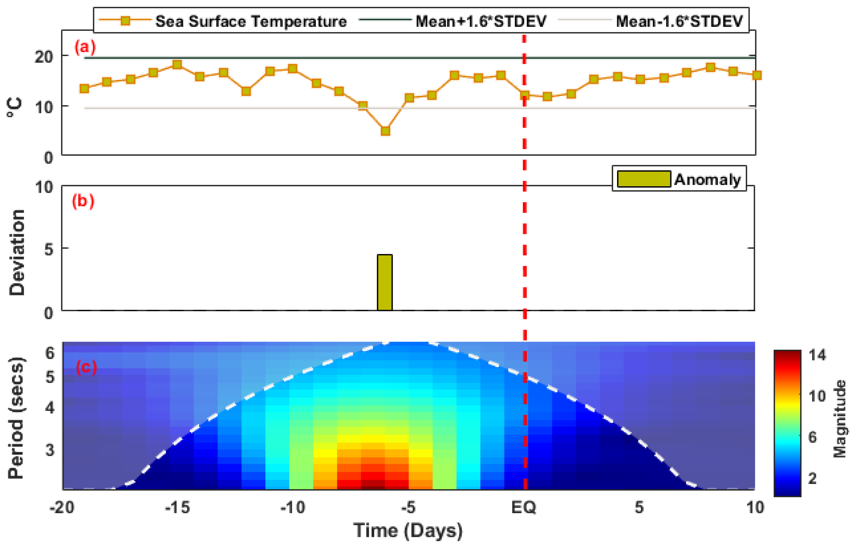
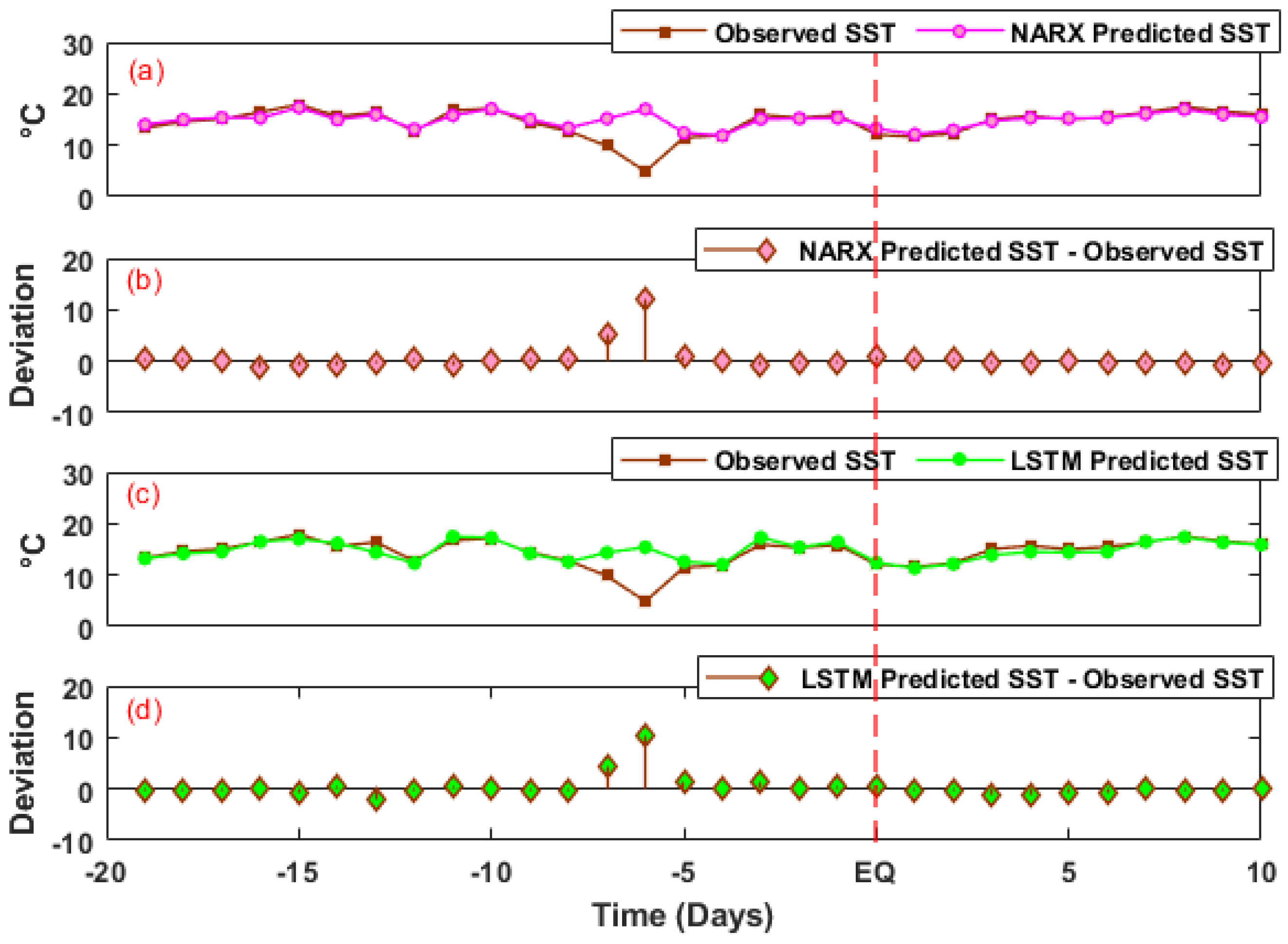
5.4. Sea Surface Temperature
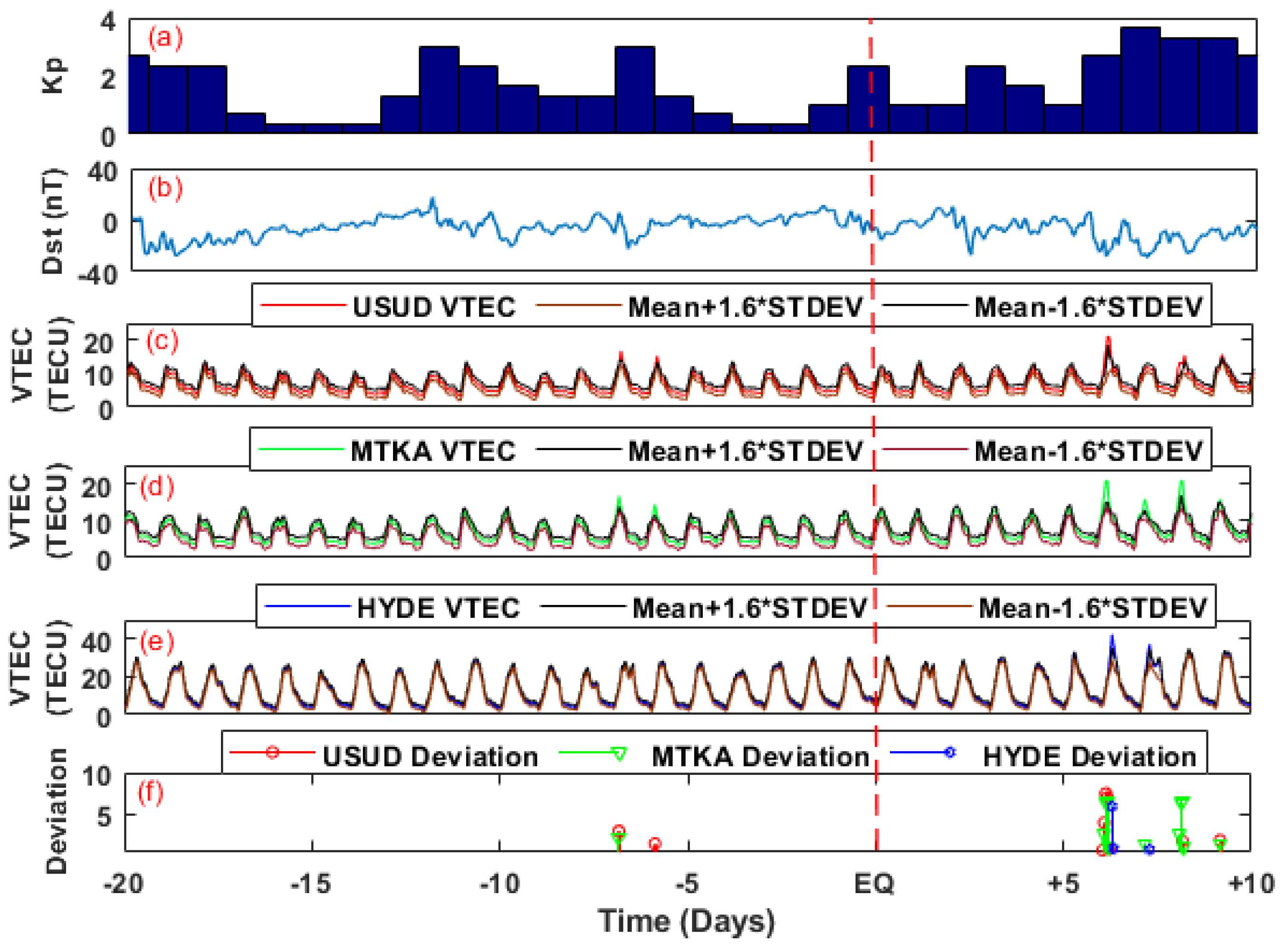
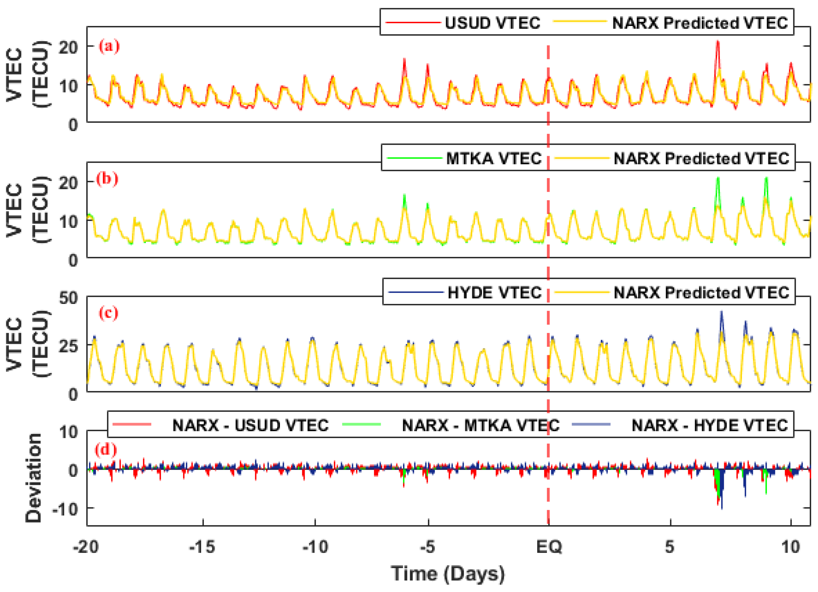
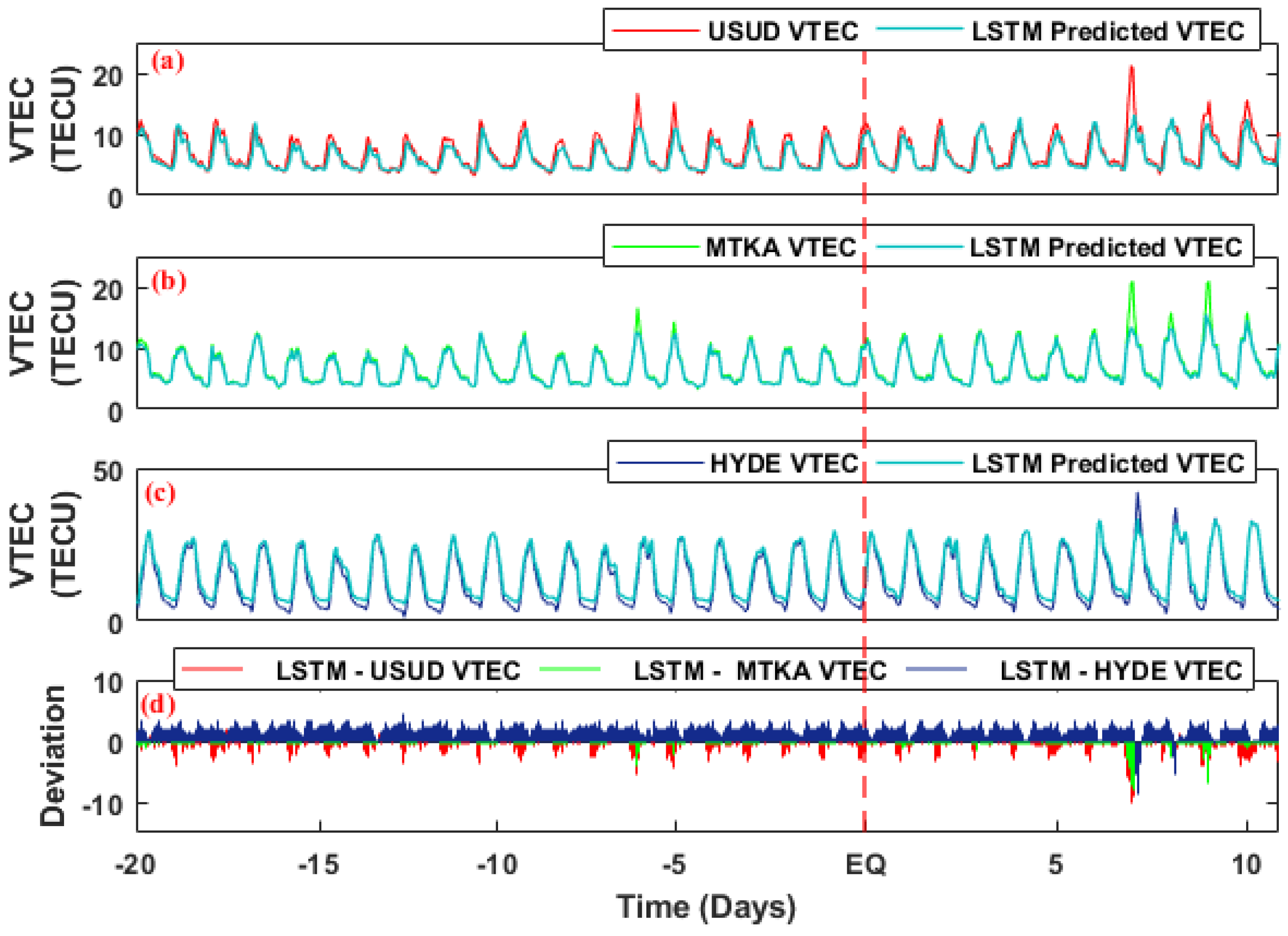
5.5. Total Electron Content
6. Discussion

| Parameters | Anomalous Day | Deviations from NARX Predicted Values | |
|---|---|---|---|
| Pre-EQ | Post-EQ | ||
| OLR (Daytime) | −6, −5 | 58, 19.8 W/m2 | Nil |
| OLR (Nighttime) | −6, −5 | 48, 6 W/m2 | Nil |
| RH (Daytime) | −6 | −15% | Nil |
| RH (Nighttime) | −6, −5 | −6, −27% | Nil |
| AT | −5 | 8 °K | Nil |
| SST | −7, −6 | −2.9, −9.7 °C | Nil |
| VTEC (USUD) | −6, −5, 7, 9 | 3.2, 2.9 TECU | 7.6, 1.7 TECU |
| VTEC (MTKA) | −6, −5, 7, 8, 9 | 3.3, 1.48 TECU | 7.3, 1.8, 6.3 TECU |
| VTEC (HYDE) | 7, 8 | Nil | 9.7, 6.47 TECU |
| Parameters | Anomalous Day | Deviations from LSTM Predicted Values | |
|---|---|---|---|
| Pre-EQ | Post-EQ | ||
| OLR (Daytime) | −6, −5 | 53.8, 26 W/m2 | Nil |
| OLR (Nighttime) | −6, −5 | 54, 9 W/m2 | Nil |
| RH (Daytime) | −6 | −15.7% | Nil |
| RH (Nighttime) | −6, −5 | −13.3, −34.5% | Nil |
| AT | −5 | 7 °K | Nil |
| SST | −7, −6 | −2, −8 °C | Nil |
| VTEC (USUD) | −6, −5, 7, 9 | 3.18, 2 TECU | 7.4, 2.1 TECU |
| VTEC (MTKA) | −6, −5, 7, 8, 9 | 3.23, 1.39 TECU | 6.5, 1.6, 5.8 TECU |
| VTEC (HYDE) | 7, 8 | Nil | 9.63, 6.32 TECU |
7. Conclusions
Author Contributions
Funding
Institutional Review Board Statement
Acknowledgments
Conflicts of Interest
References
- Blackett, M.; Wooster, M.J.; Malamud, B.D. Exploring land surface temperature earthquake precursors: A focus on the Gujarat (India) earthquake of 2001. Geophys. Res. Lett. 2011, 38, L15303. [Google Scholar] [CrossRef]
- Heki, K. Ionospheric electron enhancement preceding the 2011 Tohoku-Oki earthquake. Geophys. Res. Lett. 2011, 38, L17312. [Google Scholar] [CrossRef] [Green Version]
- Carter, B.A.; Kellerman, A.C.; Kane, T.A.; Dyson, P.L.; Norman, R.; Zhang, K. Ionospheric precursors to large earthquakes: A case study of the 2011 Japanese Tohoku Earthquake. J. Atmos. Solar-Terrestrial Phys. 2013, 102, 290–297. [Google Scholar] [CrossRef]
- Shah, M.; Jin, S. Statistical characteristics of seismo-ionospheric GPS TEC disturbances prior to global Mw ≥ 5.0 earthquakes (1998–2014). J. Geodyn. 2015, 92, 42–49. [Google Scholar] [CrossRef]
- Shah, M.; Aibar, A.C.; Tariq, M.A.; Ahmed, J.; Ahmed, A. Possible ionosphere and atmosphere precursory analysis related to Mw > 6.0 earthquakes in Japan. Remote Sens. Environ. 2020, 239, 111620. [Google Scholar] [CrossRef]
- Shah, M.; Ehsan, M.; Abbas, A.; Ahmed, A.; Jamjareegulgarn, P. Possible thermal anomalies associated with global terrestrial earthquakes during 2000–2019 based on MODIS-LST. IEEE Geosci. Remote Sens. Lett. 2021, 19, 1002705. [Google Scholar] [CrossRef]
- Shah, M.; Abbas, A.; Adil, M.A.; Ashraf, U.; de Oliveira-Júnior, J.F.; Tariq, M.A.; Ahmed, J.; Ehsan, M.; Ali, A. Possible seismo-ionospheric anomalies associated with Mw > 5.0 earthquakes during 2000–2020 from GNSS TEC. Adv. Space Res. 2022, 70, 179–187. [Google Scholar] [CrossRef]
- Venkatanathan, N.; Natyaganov, V. Outgoing longwave radiations as pre-earthquake signals: Preliminary results of 24 September 2013 (M 7.7) earthquake. Curr. Sci. 2014, 106, 1291–1297. [Google Scholar]
- Pulinets, S.; Ouzounov, D. Lithosphere–Atmosphere–Ionosphere Coupling (LAIC) model—An unified concept for earthquake precursors validation. J. Asian Earth Sci. 2011, 41, 371–382. [Google Scholar] [CrossRef]
- Liu, J.Y.; Chuo, Y.J.; Shan, S.J.; Tsai, Y.B.; Chen, Y.I.; Pulinets, S.A.; Yu, S.B. Pre-earthquake ionospheric anomalies registered by continuous GPS TEC measurements. Ann. Geophys. 2004, 22, 1585–1593. [Google Scholar] [CrossRef] [Green Version]
- Sorokin, V.M.; Pokhotelov, O.A. Model for the VLF/LF radio signal anomalies formation associated with earthquakes. Adv. Space Res. 2014, 54, 2532–2539. [Google Scholar] [CrossRef]
- Zhang, Z.-X.; Wang, C.-Y.; Shen, X.-H.; Li, X.-Q.; Wu, S.-G. Study of typical space wave—Particle coupling events possibly related with seismic activity. Chin. Phys. B 2014, 23, 109401. [Google Scholar] [CrossRef] [Green Version]
- Aleksandrin, S.Y.; Galper, A.M.; Grishantzeva, L.A.; Koldashov, S.; Maslennikov, L.; Murashov, A.M.; Picozza, P.; Sgrigna, V.; Voronov, S.A. High-energy charged particle bursts in the near-Earth space as earthquake precursors. Ann. Geophys. 2003, 21, 597–602. [Google Scholar] [CrossRef] [Green Version]
- Freund, F. Charge generation and propagation in igneous rocks. J. Geodyn. 2002, 33, 543–570. [Google Scholar] [CrossRef] [Green Version]
- Thomas, J.N.; Huard, J.; Masci, F. A statistical study of global ionospheric map total electron content changes prior to occurrences of M ≥ 6.0 earthquakes during 2000–2014. J. Geophys. Res. Space Phys. 2017, 122, 2151–2161. [Google Scholar] [CrossRef]
- Shi, K.; Guo, J.; Liu, X.; Liu, L.; You, X.; Wang, F. Seismo-ionospheric anomalies associated with Mw 7.8 Nepal earthquake on 2015 April 25 from CMONOC GPS data. Geosci. J. 2020, 24, 391–406. [Google Scholar] [CrossRef]
- Pikridas, C.; Bitharis, S.; Katsougiannopoulos, S.; Spanakaki, K.; Karolos, I.-A. Study of TEC variations using permanent stations GNSS data in relation with seismic events. Application on Samothrace earthquake of 24 May 2014. Geod. Cartogr. 2019, 45, 137–146. [Google Scholar] [CrossRef] [Green Version]
- Liu, X.; Zhang, Q.; Shah, M.; Hong, Z. Atmospheric-ionospheric disturbances following the April 2015 Calbuco volcano from GPS and OMI observations. Adv. Space Res. 2017, 60, 2836–2846. [Google Scholar] [CrossRef]
- Shah, M.; Khan, M.; Ullah, H.; Ali, S. Thermal anomalies prior to The 2015 Gorkha (Nepal) earthquake from modis land surface temperature and outgoing longwave radiations. Geodyn. Tectonophys. 2018, 9, 123–138. [Google Scholar] [CrossRef] [Green Version]
- Shah, M.; Tariq, M.A.; Ahmad, J.; Naqvi, N.A.; Jin, S. Seismo ionospheric anomalies before the 2007 M7. 7 Chile earthquake from GPS TEC and DEMETER. J. Geodyn. 2019, 127, 42–51. [Google Scholar] [CrossRef]
- Hussain, A.; Shah, M. Comparison of GPS TEC with iri models of 2007, 2012, and 1 2016 over sukkur, Pakistan. Nat. Appl. Sci. Int. J. 2020, 1, 1–10. [Google Scholar] [CrossRef] [PubMed]
- Xiong, P.; Shen, X.H.; Bi, Y.X.; Kang, C.L.; Chen, L.Z.; Jing, F.; Chen, Y. Study of outgoing longwave radiation anomalies associated with Haiti earthquake. Nat. Hazards Earth Syst. Sci. 2010, 10, 2169–2178. [Google Scholar] [CrossRef] [Green Version]
- Mohamed, E.K.; Elrayess, M.; Omar, K. Evaluation of thermal anomaly preceding northern red sea earthquake, the 16th June 2020. Arab. J. Sci. Eng. 2022, 47, 7387–7406. [Google Scholar] [CrossRef]
- Ahmed, J.; Shah, M.; Zafar, W.A.; Amin, M.A.; Iqbal, T. Seismoionospheric anomalies associated with earthquakes from the analysis of the ionosonde data. J. Atmos. Solar-Terrestrial Phys. 2018, 179, 450–458. [Google Scholar] [CrossRef]
- Shah, M.; Jin, S. Pre-seismic ionospheric anomalies of the 2013 Mw = 7.7 Pakistan earthquake from GPS and COSMIC observations. Geod. Geodyn. 2018, 9, 378–387. [Google Scholar] [CrossRef]
- Tariq, M.A.; Shah, M.; Hernández-Pajares, M.; Iqbal, T. Pre-earthquake ionospheric anomalies before three major earthquakes by GPS-TEC and GIM-TEC data during 2015–2017. Adv. Space Res. 2019, 63, 2088–2099. [Google Scholar] [CrossRef]
- Kiyani, A.; Shah, M.; Ahmed, A.; Shah, H.H.; Hameed, S.; Adil, M.A.; Naqvi, N.A. Seismo ionospheric anomalies possibly associated with the 2018 Mw 8.2 Fiji earthquake detected with GNSS TEC. J. Geodyn. 2020, 140, 101782. [Google Scholar] [CrossRef]
- Timoçin, E.; Temuçin, H.; Inyurt, S.; Shah, M.; Jamjareegulgarn, P. Assessment of improvement of the IRI model for foF2 variability over three latitudes in different hemispheres during low and high solar activities. Acta Astronaut. 2021, 180, 305–316. [Google Scholar] [CrossRef]
- Abbasi, A.R.; Shah, M.; Ahmed, A.; Naqvi, N.A. Possible ionospheric anomalies associated with the 2009 M w 6.4 Taiwan earthquake from DEMETER and GNSS TEC. Acta Geod. Geophys. 2021, 56, 77–91. [Google Scholar] [CrossRef]
- de Oliveira-Júnior, J.F.; Shah, M.; Abbas, A.; Iqbal, M.S.; Shahzad, R.; de Gois, G.; da Silva, M.V.; da Rosa Ferraz Jardim, A.M.; de Souza, A. Spatiotemporal Analysis of Drought and Rainfall in Pakistan via Standardized Precipitation Index: Homogeneous Regions, Trend, Wavelet and Influence of El Niño-Southern Oscillation. Theor. Appl. Climatol. 2022, 149, 843–862. [Google Scholar] [CrossRef]
- Khan, M.M.; Ghaffar, B.; Shahzad, R.; Khan, M.R.; Shah, M.; Amin, A.H.; Eldin, S.M.; Naqvi, N.A.; Ali, R. Atmospheric anomalies associated with the 2021 M w 7.2 Haiti earthquake using machine learning from multiple satellites. Sustainability 2022, 14, 14782. [Google Scholar] [CrossRef]
- Tariq, M.A.; Yuyan, Y.; Shah, M.; Shah, M.A.; Iqbal, T.; Liu, L. Ionospheric-Thermospheric responses to the May and September 2017 geomagnetic storms over Asian regions. Adv. Space Res. 2022, 70, 3731–3744. [Google Scholar] [CrossRef]
- Li, S.; Wang, F.; Wang, Q.; Ouyang, L.; Chen, X.; Li, J. Numerical Modeling of Branching-Streamer Propagation in Ester-Based Insulating Oil under Positive Lightning Impulse Voltage: Effects from Needle Curvature Radius. IEEE Trans. Dielectr. Electr. Insul. 2022, 30, 139–147. [Google Scholar] [CrossRef]
- Roger, J.; Pelletier, B.; Aucan, J. Update of the tsunami catalogue of New Caledonia using a decision table based on seismic data and marigraphic records. Nat. Hazards Earth Syst. Sci. 2019, 19, 1471–1483. [Google Scholar] [CrossRef] [Green Version]
- Wang, G.; Zhao, B.; Wu, B.; Wang, M.; Liu, W.; Zhou, H.; Han, Y. Research on the Macro-Mesoscopic Response Mechanism of Multisphere Approximated Heteromorphic Tailing Particles. Lithosphere 2022, 2022, 1977890. [Google Scholar] [CrossRef]
- Yue, Z.; Zhou, W.; Li, T. Impact of the Indian Ocean Dipole on Evolution of the Subsequent ENSO: Relative Roles of Dynamic and Thermodynamic Processes. J. Clim. 2021, 34, 3591–3607. [Google Scholar] [CrossRef]
- Zhong, T.; Wang, W.; Lu, S.; Dong, X.; Yang, B. RMCHN: A Residual Modular Cascaded Heterogeneous Network for Noise Suppression in DAS-VSP Records. IEEE Geosci. Remote Sens. Lett. 2022, 20, 7500205. [Google Scholar] [CrossRef]
- Chen, Y.; Zhu, L.; Hu, Z.; Chen, S.; Zheng, X. Risk Propagation in Multilayer Heterogeneous Network of Coupled System of Large Engineering Project. J. Manag. Eng. 2022, 38, 4022003. [Google Scholar] [CrossRef]
- Zhou, G.; Deng, R.; Zhou, X.; Long, S.; Li, W.; Lin, G.; Li, X. Gaussian Inflection Point Selection for LiDAR Hidden Echo Signal Decomposition. IEEE Geosci. Remote Sens. Lett. 2021, 19, 6502705. [Google Scholar] [CrossRef]
- Zhou, G.; Bao, X.; Ye, S.; Wang, H.; Yan, H. Selection of Optimal Building Facade Texture Images From UAV-Based Multiple Oblique Image Flows. IEEE Trans. Geosci. Remote Sens. 2020, 59, 1534–1552. [Google Scholar] [CrossRef]
- Huang, S.; Huang, M.; Lyu, Y. Seismic performance analysis of a wind turbine with a monopile foundation affected by sea ice based on a simple numerical method. Eng. Appl. Comput. Fluid Mech. 2021, 15, 1113–1133. [Google Scholar] [CrossRef]
- Li, R.; Yu, N.; Wang, X.; Liu, Y.; Cai, Z.; Wang, E. Model-Based Synthetic Geoelectric Sampling for Magnetotelluric Inversion with Deep Neural Networks. IEEE Trans. Geosci. Remote Sens. 2020, 60, 4500514. [Google Scholar] [CrossRef]
- Zhang, Y.; Luo, J.; Li, J.; Mao, D.; Zhang, Y.; Huang, Y.; Yang, J. Fast Inverse-Scattering Reconstruction for Airborne High-Squint Radar Imagery Based on Doppler Centroid Compensation. IEEE Trans. Geosci. Remote Sens. 2021, 60, 5205517. [Google Scholar] [CrossRef]
- Xie, X.; Xie, B.; Cheng, J.; Chu, Q.; Dooling, T. A simple Monte Carlo method for estimating the chance of a cyclone impact. Nat. Hazards 2021, 107, 2573–2582. [Google Scholar] [CrossRef]
- Xie, X.; Tian, Y.; Wei, G. Deduction of sudden rainstorm scenarios: Integrating decision makers’ emotions, dynamic Bayesian network and DS evidence theory. Nat. Hazards 2022, 45, 5303435. [Google Scholar] [CrossRef]
- Zhu, X.; Xu, Z.; Liu, Z.; Liu, M.; Yin, Z.; Yin, L.; Zheng, W. Impact of dam construction on precipitation: A regional perspective. Mar. Freshw. Res. 2022, 63, 23–32. [Google Scholar] [CrossRef]
- Schaer, S. Mapping and Predicting the Earth’s Ionosphere Using the Global Positioning System; Schweizerische Geodätische Kommission: Zürich, Switzerland, 1999; Volume 59. [Google Scholar]
- Dobrovolsky, I.P.; Zubkov, S.I.; Miachkin, V.I. Estimation of the size of earthquake preparation zones. Pure Appl. Geophys. 1979, 117, 1025–1044. [Google Scholar] [CrossRef]
- Akyol, A.A.; Arikan, O.; Arikan, F. A machine learning-based detection of earthquake precursors using ionospheric data. Radio Sci. 2020, 55, 1–21. [Google Scholar] [CrossRef]
- Al Ibrahim, M.; Park, J.; Athens, N. Earthquake Warning System: Detecting Earthquake Precursor Signals Using Deep Neural Networks; Stanford University Press: Redwood City, CA, USA, 2018; p. 230. [Google Scholar]
- Ouzounov, D.; Liu, D.; Chunli, K.; Cervone, G.; Kafatos, M.; Taylor, P. Outgoing long wave radiation variability from IR satellite data prior to major earthquakes. Tectonophysics 2007, 431, 211–220. [Google Scholar] [CrossRef]
- Jing, F.; Shen, X.H.; Kang, C.L.; Xiong, P. Variations of multi-parameter observations in atmosphere related to earthquake. Nat. Hazards Earth Syst. Sci. 2013, 13, 27–33. [Google Scholar] [CrossRef] [Green Version]
- Walker, R.; Jackson, J. Offset and evolution of the Gowk fault, SE Iran: A major intra-continental strike-slip system. J. Struct. Geol. 2002, 24, 1677–1698. [Google Scholar] [CrossRef]
- Hereher, M.; Bantan, R.; Gheith, A.; El-Kenawy, A. Spatio-temporal variability of sea surface temperatures in the Red Sea and their implications on Saudi Arabia coral reefs. Geocarto Int. 2022, 37, 5636–5652. [Google Scholar] [CrossRef]
- Shah, M.; Qureshi, R.U.; Khan, N.G.; Ehsan, M.; Yan, J. Artificial Neural Network based thermal anomalies associated with earthquakes in Pakistan from MODIS LST. J. Atmos. Solar-Terrestrial Phys. 2021, 215, 105568. [Google Scholar] [CrossRef]
- Freund, F.T.; Takeuchi, A.; Lau, B.W.S.; Al-Manaseer, A.; Fu, C.C.; Bryant, N.A.; Ouzounov, D. Stimulated infrared emission from rocks: Assessing a stress indicator. eEarth 2007, 2, 7–16. [Google Scholar] [CrossRef] [Green Version]
- Shah, M.; Abbas, A.; Ehsan, M.; Aiber, A.C.; Adhikari, B.; Tariq, M.A.; Ahmed, J.; de Oliveira-Júnior, J.F.; Yan, J.; Melgarejo-Morales, A.; et al. Ionospheric--thermospheric responses in south America to the august 2018 geomagnetic storm based on multiple observations. IEEE J. Sel. Top. Appl. Earth Obs. Remote Sens. 2021, 15, 261–269. [Google Scholar] [CrossRef]
- Ondoh, T. Anomalous sporadic-E layers observed before M7.2 Hyogo-ken Nanbu earthquake; Terrestrial gas emanation model. Adv. Polar Upper Atmos. Res. 2003, 17, 96–108. [Google Scholar]
- Tariq, M.A.; Shah, M.; Inyurt, S.; Shah, M.A.; Liu, L. Comparison of TEC from IRI-2016 and GPS during the low solar activity over Turkey. Astrophys. Space Sci. 2020, 365, 179. [Google Scholar] [CrossRef]
- Yin, L.; Wang, L.; Tian, J.; Yin, Z.; Liu, M.; Zheng, W. Atmospheric Density Inversion Based on Swarm-C Satellite Accelerometer. Appl. Sci. 2023, 13, 3610. [Google Scholar] [CrossRef]
- Liu, Z.; Xu, J.; Liu, M.; Yin, Z.; Liu, X.; Yin, L.; Zheng, W. Remote sensing and geostatistics in urban water-resource monitoring: A review. Mar. Freshw. Res. 2023, 82, 34–45. [Google Scholar] [CrossRef]
- Zhang, S.; Bai, X.; Zhao, C.; Tan, Q.; Luo, G.; Wang, J.; Li, Q.; Wu, L.; Chen, F.; Li, C.; et al. Global CO2 Consumption by Silicate Rock Chemical Weathering: It’s past and Future. Earth’s Future 2021, 9, e1938E–e2020E. [Google Scholar] [CrossRef]
- Cheng, Y.; Fu, L.-Y. Nonlinear seismic inversion by physics-informed Caianiello convolutional neural networks for overpressure prediction of source rocks in the offshore Xihu depression, East China. J. Pet. Sci. Eng. 2022, 215, 110654. [Google Scholar] [CrossRef]
- Shahzad, F.; Shah, M.; Riaz, S.; Ghaffar, B.; Ullah, I.; Eldin, S.M. Integrated Analysis of LithosphereAtmosphere-Ionospheric Coupling Associated with the 2021 Mw 7.2 Haiti Earthquake. Atmosphere 2023, 14, 347. [Google Scholar] [CrossRef]
- Shah, M.; Shahzad, R.; Ehsan, M.; Ghaffar, B.; Ullah, I.; Jamjareegulgarn, P.; Hassan, A.M. Seismo Ionospheric Anomalies around and over the Epicenters of Pakistan Earthquakes. Atmosphere 2023, 14, 601. [Google Scholar] [CrossRef]


| Parameters | Anomalous Day | Deviations from UB and LB | |
|---|---|---|---|
| Pre-EQ | Post-EQ | ||
| OLR (Daytime) | −6, −5 | 36, 11.4 W/m2 | Nil |
| OLR (Nighttime) | −6 | 18 W/m2 | Nil |
| RH (Daytime) | −6 | −8% | Nil |
| RH (Nighttime) | −5 | −6% | Nil |
| AT | −5 | 2 °K | Nil |
| SST | −6 | −4.5 °C | Nil |
| VTEC (USUD) | −6, −5, 7, 9 | 3, 1.5 TECU | 7.5, 1.8 TECU |
| VTEC (MTKA) | −6, −5, 7, 8, 9 | 2.32, 0.5 TECU | 6.6, 1.5, 6.7 TECU |
| VTEC (HYDE) | 7, 8 | Nil | 5.95, 0.8 TECU |
Disclaimer/Publisher’s Note: The statements, opinions and data contained in all publications are solely those of the individual author(s) and contributor(s) and not of MDPI and/or the editor(s). MDPI and/or the editor(s) disclaim responsibility for any injury to people or property resulting from any ideas, methods, instructions or products referred to in the content. |
© 2023 by the authors. Licensee MDPI, Basel, Switzerland. This article is an open access article distributed under the terms and conditions of the Creative Commons Attribution (CC BY) license (https://creativecommons.org/licenses/by/4.0/).
Share and Cite
Draz, M.U.; Shah, M.; Jamjareegulgarn, P.; Shahzad, R.; Hasan, A.M.; Ghamry, N.A. Deep Machine Learning Based Possible Atmospheric and Ionospheric Precursors of the 2021 Mw 7.1 Japan Earthquake. Remote Sens. 2023, 15, 1904. https://doi.org/10.3390/rs15071904
Draz MU, Shah M, Jamjareegulgarn P, Shahzad R, Hasan AM, Ghamry NA. Deep Machine Learning Based Possible Atmospheric and Ionospheric Precursors of the 2021 Mw 7.1 Japan Earthquake. Remote Sensing. 2023; 15(7):1904. https://doi.org/10.3390/rs15071904
Chicago/Turabian StyleDraz, Muhammad Umar, Munawar Shah, Punyawi Jamjareegulgarn, Rasim Shahzad, Ahmad M. Hasan, and Nivin A. Ghamry. 2023. "Deep Machine Learning Based Possible Atmospheric and Ionospheric Precursors of the 2021 Mw 7.1 Japan Earthquake" Remote Sensing 15, no. 7: 1904. https://doi.org/10.3390/rs15071904