Article

Accuracy Enhancement and Feature Extraction for GNSS Daily Time Series Using Adaptive CEEMD-Multi-PCA-Based Filter

Shandong Provincial Key Laboratory of Geomatics and Digital Technology of Shandong Province, Shandong University of Science and Technology, Qingdao 266590, China
*
Author to whom correspondence should be addressed.
Remote Sens. 2023, 15(7), 1902; https://doi.org/10.3390/rs15071902
Submission received: 10 March 2023 / Revised: 27 March 2023 / Accepted: 27 March 2023 / Published: 1 April 2023
(This article belongs to the Special Issue Remote Sensing in Space Geodesy and Cartography Methods)

Abstract

:
Global navigation satellite system (GNSS) positions include various useful signals and some unmodeled errors. In order to enhance the accuracy and extract the features of the GNSS daily time sequence, an improved method of complete ensemble empirical mode decomposition (CEEMD) and multi-PCA (MPCA) based on correlation coefficients and block spatial filtering was proposed. The results showed that the mean standard deviations of the raw residual time sequence were 1.09, 1.20 and 4.79 mm, while those of the newly proposed method were 0.15, 0.20 and 2.86 mm in north, east and up directions, respectively. The proposed method outperforms wavelet decomposition (WD)-PCA and empirical mode decomposition (EMD)-PCA in effectively eliminating low- and high-frequency noise, and is suitable for denoising nonlinear and nonstationary GNSS position sequences. Furthermore, feature extraction of the denoised GNSS daily time series was based on CEEMD, which is superior to WD and EMD. Results of noise analysis suggested that the noise components in the original and denoised GNSS time sequence are complex. The advantages of the proposed method are the following: (i) it fully exploits the merits of CEEMD and WD, where CEEMD is first used to obtain the limited intrinsic modal functions (IMFs) and then to extract seasonal and trend features; (ii) it has good adaptive processing ability via WD for noise-dominant IMFs; and (iii) it fully considers the correlation between the different components of each station and the non-uniform behavior of common mode error on a spatial scale.

1. Introduction

In recent decades, owing to the rapid development of Global Navigation Satellite System (GNSS) technology and the continuous accumulation of observational data, a significant amount of data pertaining to crustal movement velocity fields and crustal deformation in plate boundary regions have been acquired. These data have been applied in geophysics, atmospheric science and dynamic displacement detection during natural disasters [1,2,3,4,5,6,7]. However, the GNSS position time sequence includes not only crustal deformation signals, but also non-tectonic deformation signals and several systematic errors [8,9,10,11,12]. Various error sources affect GNSS positioning accuracy. Researchers have proposed various techniques to calculate the parameters of the GNSS signal time series and the associated noise [13,14]. Research findings indicate that random fluctuations of the GNSS position time series, typically termed as noise, can be represented by a combination of white noise (WN) and power-law (PL) processes [15].
Owing to the superposition of all types of “signals” and “noises” in GNSS coordinate time series, seasonal variations are apparent [16,17,18,19], which include geophysical signals and systematic errors from various sources. To accurately classify GNSS signals into crustal movement and other signals and achieve dependable long-term motion trends, seasonal signals must be estimated and must be obtained accurately [20]. Moreover, a common mode error (CME) is evident between GNSS sites, i.e., the positional error generated by the common movement of the GNSS sites [9,10,21]. Hence, the quality of GNSS observations is affected significantly by these errors, which may result in inaccurate interpretations or biased estimations of geophysical events.
To date, various spatiotemporal filtering methods have been proposed to reduce the CME at GNSS positions, including stacking filtering (STK) [9,10] and principal component analysis (PCA) [12,22]. STK is easy to compute but is only applicable to small-scale, uniformly distributed GNSS networks. PCA can be applied to reduce data dimensions and extract data correlations; however, during denoising, the primary principal components cannot be obtained, and some signal information can be lost. For the GNSS daily coordinate time series, Dong et al. [11] performed PCA and the Karhunen–Loeve expansion to identify signals and unmodeled systematic errors. The results showed that one of the dominant error sources was spatiotemporally correlated with the CME in the GNSS long-term coordinate time series. However, PCA is effective only if the CME exhibits an almost uniform behavior, which is based on the fact that on a certain spatial scale, the CME exhibits a non-uniform behavior. Furthermore, PCA is mainly used to weaken the systematic colored noise in GNSS residual signals, whereas it cannot remove WN noise in the signals.
Although the methods discussed above can reduce the noise in GNSS positions to some degree, they do not perform any decomposition but rather process GNSS datasets in a single dimension, whereas GNSS data are multi-scale in nature; thus the signals cannot be decomposed into different time scales. As a new analytical method for time-frequency localization, the wavelet transform (WT) [23,24,25] can decompose the original signal, obtain the general situation of the signal on a large scale and obtain details regarding the signal on a small scale. It is widely used in signal analysis and noise elimination [26]. Although WT performs well in smoothing noise, no accurate method exists for identifying the wavelet base and decomposition level. The pre-divided time and frequency characteristics of the WT hamper its capacity to adaptively decompose signals into various time frequencies based on the intrinsic features of signals; it is mainly used to eliminate high-frequency random noise, but with low efficiency in eliminating low-frequency colored noise. Based on the merits of WT and PCA, Bakshi [27] proposed a WT-based multi-scale PCA (MSPCA), which proved to be highly efficient in multivariate monitoring. However, when denoising GNSS positions, MSPCA considers only the correlations between the same position directions at different sites, whereas the spatial correlation between the components of the coordinates for all sites is disregarded. Singular spectrum analysis (SSA) [28] is effective for managing signals with small time-domain waveform fluctuations. Moreover, for signals with significant fluctuations, the appropriate noise platform parameters should be selected to significantly reduce noise. However, the selection rules for the noise platform parameters are not clearly defined [29]. Jin et al. [30] used a method combining empirical mode decomposition (EMD) and SSA to estimate the nonlinear trend terms in the time series of actual sea level changes with high accuracy and consistency. Kong et al. [31] performed an SSA and a Fourier fast transform to analyze a long-term polar motion time sequence obtained via Doppler orbitography and radio positioning integrated by satellite observations.
Many methods based on time-scale decomposition have been developed. Shen et al. [32] used variational mode decomposition (VMD) combined with a correlation coefficient to denoise the original sequence and extract seasonal, trend, and residual terms. Xu et al. [33] proposed a type of energy entropy mutual information as the objective function to improve VMD combined with a wavelet packet denoising algorithm, to address inadequate decomposition or to effectively denoise the time series. Montillet et al. [34] used the EMD algorithm to decompose the GPS coordinate time series into a series of sub-time series, and then proposed an algorithm to estimate the Hurst parameter for each sub-time series to calculate the statistics of WN. He et al. [12] performed PCA to a process based on spatial filtering to enhance the accuracy and reliability of GNSS position time series. Lu et al. [35] proposed an EMD-PCA combined method to reduce the multipath effect and high-frequency random noise. He et al. [36] developed a MATLAB-based denoising software named GNSS-TS-NRS, which can denoise signals using five methods, including EMD and ensemble EMD, and can effectively perform signal processing. Lee et al. [37] used EMD and PCA to detect climate change signals to weaken the effect of background noise and increase their ability to detect climate change. Zhang et al. [38] proposed a wavelet decomposition (WD)-PCA combined method to improve the vulnerability of PCA to high-frequency random noise in daily coordinate sequences and effectively improved positioning accuracy. Lu et al. [39] proposed a GPS time series prediction model based on complete ensemble empirical mode decomposition (CEEMD). Based on the model identification rules, each intrinsic modal function (IMF) and residual should be modeled separately, and the final predicted results of the GPS time series can be calculated. For GPS multipath error extraction, Long et al. [40] proposed a new algorithm based on the CEEMD-wavelet-SavGol model to address the mode-mixing effect of the EMD algorithm and the limitations of wavelet denoising. Li et al. [41] developed CEEMD-multi-PCA (CEEMD-MPCA) combined with a correlation coefficient to increase the accuracy and feature extraction of GNSS coseismic positions with a high sampling rate. The CEEMD-MPCA denoising method is not only suitable for the seismic feature extraction of GNSS seismic positions, but also eliminates WN and systematic errors while retaining earthquake waveforms with high performance by considering the correlation among the different components of each station.
To enhance the reliability of GNSS positioning and feature extraction, an adaptive method using CEEMD-MPCA based on correlation coefficients and block spatial filtering is proposed herein. Compared with previous studies, our study offers the following advantages: (i) the CEEMD method is first applied to decompose the GNSS time series into various IMFs based on the inherent time-scale features of the data; (ii) the proposed approach based on MPCA fully considers correlations among different components of each station and the non-uniform behavior of the CME on a spatial scale; and (iii) the CEEMD method is applied to the trend- and seasonal-feature extraction of the denoised GNSS time series.
The remainder of this paper is organized as follows. The GNSS daily time series and processing process are presented in Section 2. Section 3 describes the methodological procedures and principles of the analysis. In Section 4, noise analysis based on Hector software is presented. Finally, the conclusions are presented in Section 5.

2. GNSS Daily Time Series and Preprocessing Procedure

The International GNSS Service (IGS) is a high-precision international GNSS product (https://www.igs.org/about/, accessed on 8 March 2023). Currently, approximately 506 continuously operating GNSS sites are globally distributed and use data from these sites to publish satellite orbits, satellite clocks, zenith path delays, zenith tropospheric delays and other products. The IGS comprises three global data centers: the Crustal Dynamics Data Information System, the South Orange Performing Arts Center and the Institut Géographique National, which can provide pseudo-range and phase observations, broadcast ephemeris and meteorological data free of charge. The SOPAC uses “st_filter” software (http://sopac-ftp.ucsd.edu/pub/timeseries/measures/, accessed on 8 March 2023) to combine constrained solutions from the JPL and SOPAC analysis centers, remove the errors caused by software and processing schemes and derive a consistent solution. The solution strategy adopted by the analysis center and the error model used are details that can be found on the SOPAC website (http://garner.ucsd.edu/pub/measuresESESES_products/ATBD/, accessed on 8 March 2023).
The SOPAC provides three types of data: raw, clean and filtered. Among them, “clean” daily time series data are generated by the removal of outliers, mean and coseismic and non-seismic jumps from the original data. The gaps for a few missing epochs are filled using linear interpolation. In theory, the daily time series of a “clean trend” location contains trends, seasonal signals and spatial correlation noise.
The accuracy of the newly proposed method was assessed using a GNSS daily coordinate time sequence in a 10-year span from 27 October 2010 to 27 October 2020, at 20 sites in the SOPAC network (Figure 1). The selected 20 stations were categorized into two blocks (10 GNSS stations in central California (Block 1) and 10 stations in southern California (Block 2)). This selection was based on the following considerations: First, He et al. [12] showed that in the GNSS region, block-space filtering can weaken seasonal variation, reduce regional effects and enhance the accuracy and reliability of GNSS data. Second, to obtain accurate trends from continuous time sequences, the time span must be at least 2.5 years [4,42]. Finally, the selected IGS stations have a low data loss rate, as shown in Table 1, for the 20 stations; the average data loss rates for Blocks 1 and 2 were 0.98% and 1.81%, respectively (Table 1). The low data loss rate renders it possible to analyze the GNSS time series in both time and frequency domains. Furthermore, the 10-year observation period was sufficient to obtain accurate trends.
The daily GNSS coordinate time sequences and other relevant parameters were obtained for each site. The GNSS time sequence at station P242 is shown in Figure 2. Site P242 exhibited a long-trend term of moving northeast (Figure 2a), and the mean root mean squares of the GNSS residue were 1.46, 1.64 and 4.67 mm in the north (N), east (E) and up (U) directions, respectively (Figure 2b), with clear seasonal variation and primarily annual trends, particularly in the north and up components.

3. Methods

3.1. An Improved Denoising Method for GNSS Daily Time Series

The definitions of the CEEMD method, correlation coefficient between each IMF and raw signal are provided in Equations (A1) and (A2) in the Appendix A. Based on the methods mentioned in the appendix, an improved method involving CEEMD-MPCA combined with the correlation coefficient and block spatial filtering was developed to enhance the accuracy of the GNSS daily coordinate time sequence and feature extraction. In this method, the selected GNSS network is classified into several blocks. The three-dimensional daily GNSS data matrix is converted into a two-dimensional matrix, which is used to decompose the GNSS daily coordinate time sequence into limited IMFs. The inflection point of the transitional IMF is determined using the correlation coefficient. Wavelet denoising is performed to filter the former noise-dominated mode, and the filtered signal is reconstructed using the remaining matrix. Finally, MPCA is performed to reconstruct and process the processed IMF to obtain the denoised time sequence. The details of the improved method are as follows:
(i)
The GNSS network is classified into several blocks based on the scale or range while considering the spatial distribution of the GNSS stations.
(ii)
The three-dimensional GNSS data matrix S ¯ ( m ,   n ,   q ) is converted into a two-dimensional GNSS data matrix S ( n ,   u ) ,   u = m   ×   q , where n, m and q represent the number of epochs, selected station and coordinate directions of each site, respectively. The three coordinate components in order are N, E and U.
(iii)
Each column in matrix S ( n ,   u ) is adaptively decomposed into K IMFs based on the frequency level using the CEEMD method.   I M F s = { i m f j , 1 , i m f j , 2 , , i m f j , K } , j = 1 ,   2 ,   ,   u .
(iv)
The CCs between the raw residual time sequence and each IMF are calculated, and the corresponding matrix   C C s = { c c j , 1 , c c j , 2 , , c c j , K } are obtained. Starting from cc j , 1 , the IMF component i m f j , h corresponds to the first extreme value c c j , h in the CCs, and the next IMF component i m f j , h + 1 is the transitional IMF.
(v)
The transition IMF (noise-dominant) and noise IMFs are combined into a new matrix X D = { x d j , 1 , x d j , 2 , , x d j , h + 1 } , and each column of matrix X D is processed via wavelet denoising; subsequently, the new matrix X R = { x r j , 1 , x r j , 2 , , x r j , h + 1 } is obtained after denoising.
(vi)
The denoised matrix X R and monochromatic IMFs are reconstructed to obtain a new matrix X E = { x e 1 x e 2 , , x e n } . MPCA is applied to matrix X E and the value of cumulative contribution rate (CCR) of the first k components is calculated.
(vii)
If the value of CCR exceeds 85%, then the top k components are selected as the denoised signals, and a new denoised matrix X F = { x f 1 ,   x f 2 , ,   x f n } is reconstructed.

3.2. Feature Extraction of Seasonal and Trend Terms

The fundamental step in data analysis is to determine and remove nonlinear trend terms from the data [41]. Based on EMD, the trend term is defined as follows: the trend for a dataset with a certain time range is a function that has, at the maximum, one extreme value or a monotone function with inherent determination [43].
One of the most evident features of the GNSS daily time sequence is the seasonal term, which is primarily caused by the migration of surface materials, including surface water, snow cover, vegetation changes, and tides [44,45]. Many early studies showed that the seasonal terms of the sequence are mainly composed of semi-annual and annual cycle terms [46,47].
After performing denoising using the proposed method, the denoised matrix X F is used as the starting input matrix. Subsequently, CEEMD is applied to obtain the trend and seasonal terms. The corresponding feature extraction results are calculated as follows:
X F = I SEA + I TRE + R E S
where ISEA represents the seasonal term of the denoised data results obtained via CEEMD, ITRE represents the trend term extracted from the denoised data and RES represents the residuals. The structure of the proposed method is shown in Figure 3.

4. Results and Analysis

4.1. Results of GNSS Denoised Data

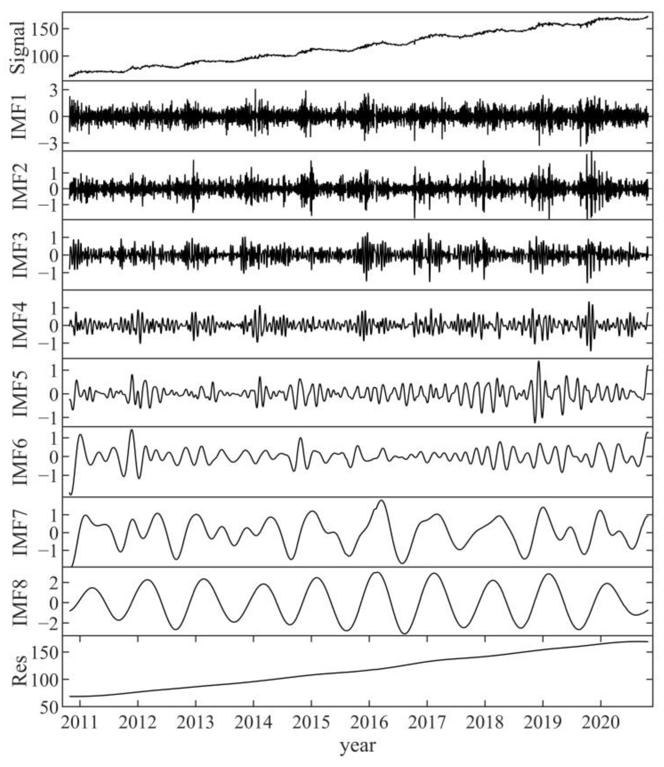
Herein, the N component of site P242 is presented as an example to assess the proposed method. The GNSS coordinate time series were first decomposed using CEEMD into different IMFs, and the decomposition results for the eight IMFs and one residue were obtained (Figure 4). IMF 8 shows a clear annual variation in the GNSS daily time series, whereas IMF 7 shows a strong seasonal cycle.
Table 2 shows the CCs between the raw north GNSS time sequence of station P242 and each IMF decomposed by CEEMD. The transitional IMF was IMF5. Based on our method, IMF1–IMF4 are “noise-dominant” IMFs, IMF5 is a “transition” IMF and the remaining IMFs are “signal-dominant” IMFs. IMF1–IMF5, as “noise-dominant” models, were combined into a new matrix X D = { x d j , 1 , x d j , 2 , , x d j , 5 } ,   j = 1 ,   2 ,   ,   u . For every column of wavelet soft threshold denoising processing, a new matrix X R = { x r j , 1 , x r j , 2 , , x r j , 5 } was obtained. The denoised matrix and “signal-dominant” IMFs were reconstructed to obtain a new matrix X E . The MPCA method was used for matrix X E , and the top k components, where the cumulative contribution rate of the first k components exceeded 85%, were selected. The final denoised matrix X F was reconstructed.
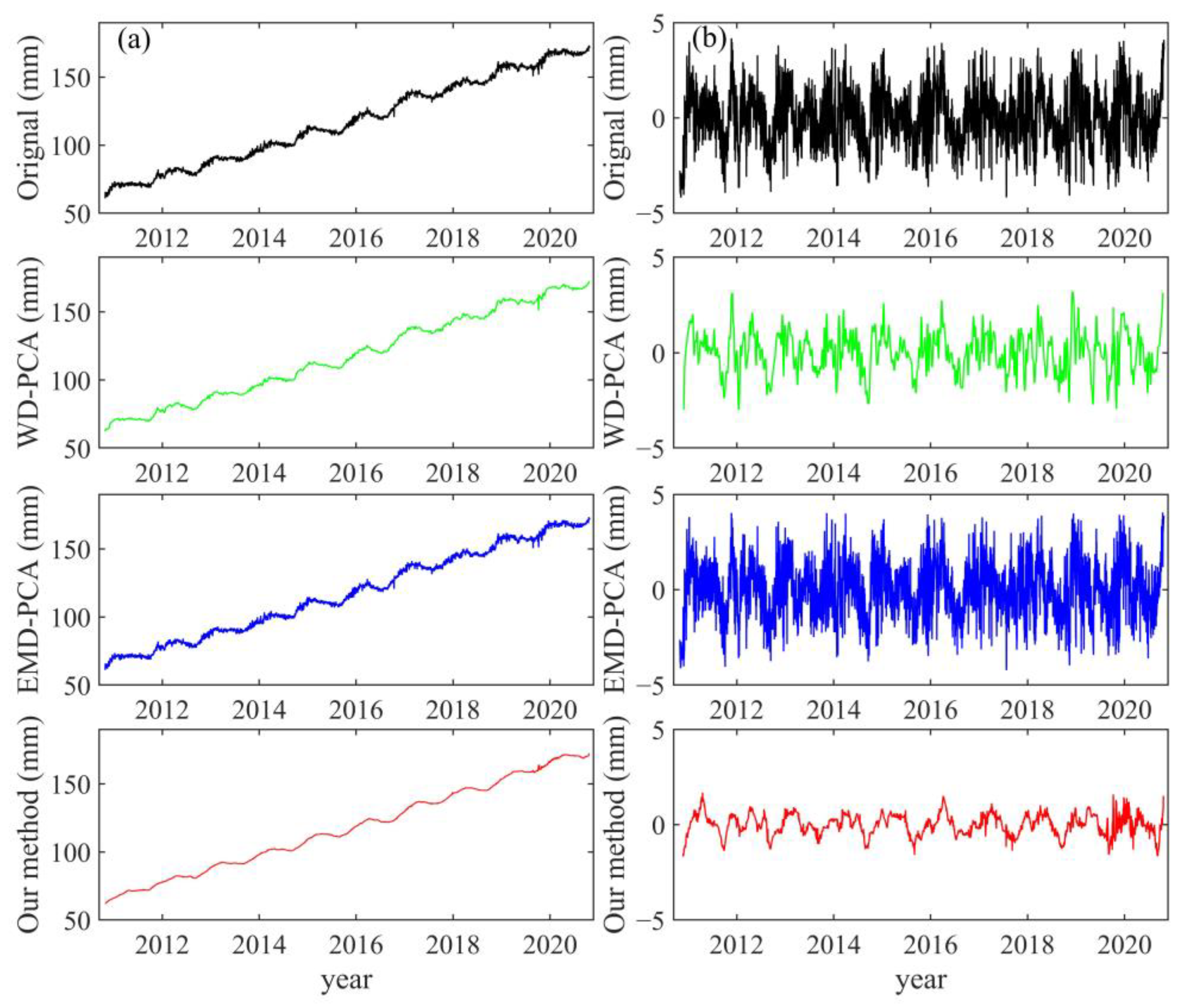
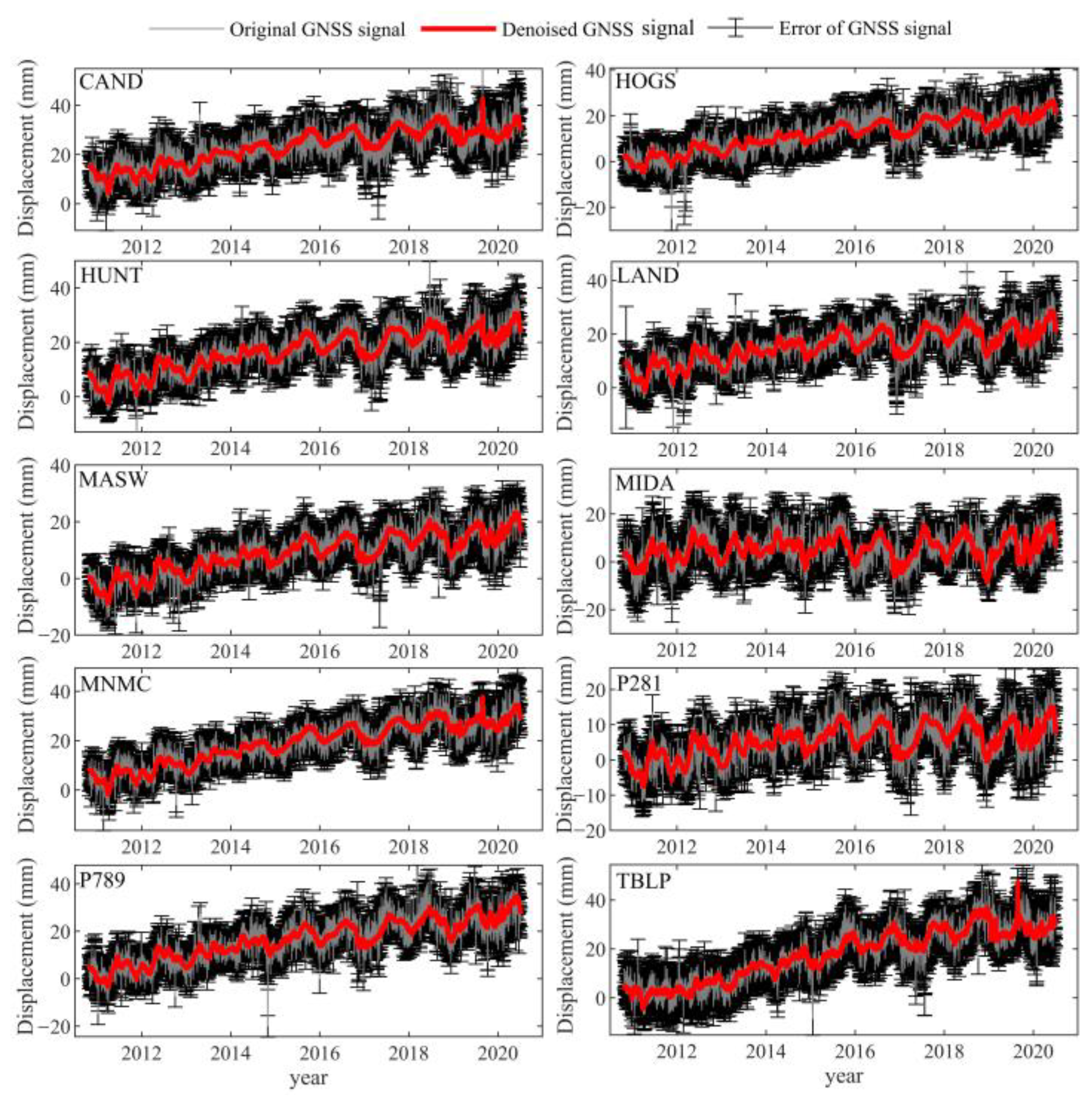
The raw and denoised GNSS coordinate time sequence at station P242 in the N direction and their corresponding residual time series are shown in Figure 5. Clear nonlinear variations and oscillations with time were exhibited in the raw coordinate time series, which indicates that the raw GNSS time series was affected by WN, and the colored noise was nonlinear and nonstationary (Figure 5a). The proposed method was smoother than WD-PCA and EMD-PCA, indicating that the proposed method not only effectively eliminated noise at high frequencies, but also reduced noise at low frequencies. Nonlinear oscillations and random fluctuations with high frequencies were observed in the raw residual time series (Figure 5b), indicating the presence of WN with high frequencies and systematic noise with low frequencies in the raw GNSS daily coordinate sequence. The proposed method can eliminate more noise at both high and low frequencies than WD-PCA and EMD-PCA. WD-PCA considers the advantages of wavelet denoising and PCA in removing noise at both high and low frequencies. Meanwhile, EMD-PCA considers the advantages of EMD and PCA in partially removing low-frequency noise. Furthermore, the proposed method combines the advantages of CEEMD-WD and MPCA, which consider the correlation between all directions of the station and eliminate various noises effectively. CEEMD is more accurate than the other methods because of its highly adaptive and data-driven ability to decompose GNSS datasets into IMFs of different frequencies.
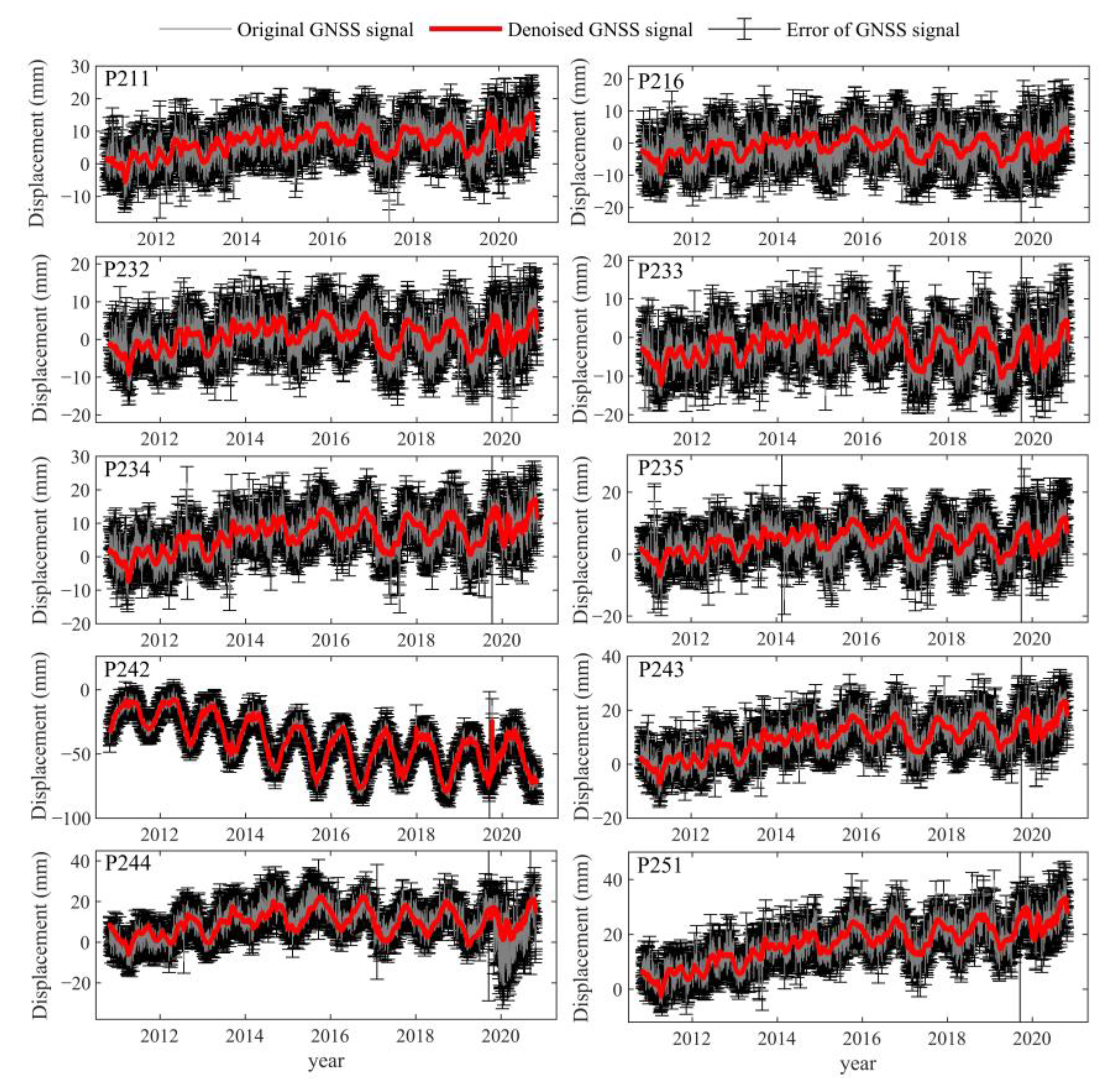
To analyze the denoising effect more comprehensively using the proposed method, the raw and denoised GNSS coordinate time sequences in the U direction for Blocks 1 (Figure 6) and 2 (Figure A1) are shown. The raw GNSS daily time sequence contains centimeter-level fluctuations, namely low-frequency colored noise and clear random oscillations with high frequencies. The denoised coordinate time series was much smoother than the original time series, indicating that the denoising effect is better. For example, the time series of station P242 shows apparent annual cycles, which may be due to changes in the surface environment composed of sea level, continental water and atmospheric load changes, thus resulting in periodic changes in crustal deformation [44,48].
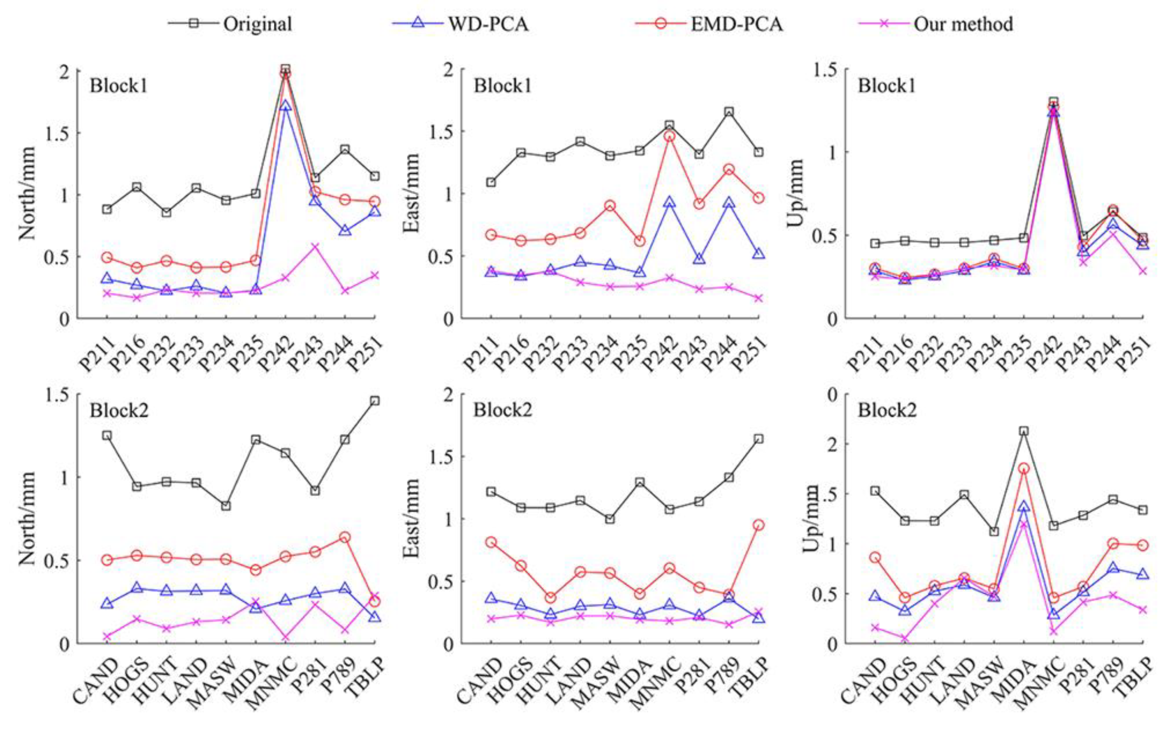
To quantitatively describe the improvement in the accuracy of the GNSS daily positions, the standard deviations (STDs) of the GNSS residual time sequences of various methods at each station are shown in Figure 7. Regardless of the block, the STDs of the original data were the highest. The EMD-PCA method exhibited the least improvement in terms of accuracy, whereas the proposed method exhibited the most significant improvement.
For Block 1, the horizontal components of the proposed method were significantly better than the up component of the other methods. For the N component, the STDs of the original residual data, WD-PCA, EMD-PCA and the proposed method were [0.86–2.02], [0.20–1.71], [0.41–1.98] and [0.17–0.58], respectively. For the E component, the STDs of the original residual time series, WD-PCA, EMD-PCA and the proposed method were [1.09–1.66], [0.34–0.93], [0.62–1.46] and [0.16–0.38], respectively. The proposed approach exhibited a significantly higher accuracy than the other approaches in the horizontal direction because the coordinate time sequences of each station in the horizontal direction indicated a stronger correlation, and MPCA can theoretically fully utilize the correlation between different coordinate components to remove noise (Figure 7). In the up direction, the accuracies achieved by the three methods for stations P216, P232, P233, P235 and P242 were similar. At the remaining stations, the proposed method exhibited a slightly higher accuracy than the other methods. The STD ranges of the original residual time series, WD-PCA, EMD-PCA and C-MPCA data were [4.50–13.02], [2.29–12.36], [2.45–12.71] and [2.35–12.46], respectively, because the correlation between the U components of each station was weak. Considering the correlation between different coordinate components, the filtering effect in the U component was not significant.
For Block 2, the proposed approach showed higher accuracy in the northern regions than the other approaches, except for the MIDA and TBLP stations. For the N component, the STDs of the original residual data, WD-PCA, EMD-PCA and the proposed method were [0.83–1.46], [0.15–0.33], [0.25–0.64] and [0.04–0.29], respectively. The median error of the proposed method exceeded that of the WD-PCA method, which was mainly due to the inferior decomposition effect of CEEMD at this station, which resulted in the low filtering accuracy of these two stations. In the east direction, except for TBLP station, the accuracy of the proposed method exceeded that of the other methods. For the E component, the STD ranges of data obtained by the original residual time series, WD-PCA, EMD-PCA and the proposed method were [1.00–1.64], [0.20–0.36], [0.37–0.95] and [0.15–0.26], respectively. For the U component, the STD ranges of the raw residual data, WD-PCA, EMD-PCA and C-MPCA were [4.24–6.26], [2.54–4.73], [2.92–5.51] and [2.11–4.40], respectively. For the LAND and MASW stations, the WD-PCA method performed slightly better than the EMD-PCA and the proposed method, whereas for the other stations, the proposed method performed better than the other methods. This is because the correlation between the U components of each station was weak. Considering the correlation between different coordinate components, the filtering effect of the upper components was not significant.
Table 3 presents the mean STD in each direction for the overall, Block 1 and Block 2 regions. For the overall denoising, the average STDs of the original residual data, WD-PCA and EMD-PCA in the N, E and U directions were (1.12, 1.28, 5.25) mm, (0.45, 0.53, 3.70) mm and (0.56, 0.68, 3.91) mm, respectively. However, the average STDs of the proposed approach were 0.31, 0.30, 3.46 mm in the N, E and U directions, respectively. Furthermore, after separating the GNSS network into two blocks by determining each block’s scale or range and considering the spatial distribution of the GNSS stations, for Block 1 region in the N, E and U directions, the average STDs of the raw residual data, WD-PCA and EMD-PCA were (1.15, 1.36, 5.70) mm, (0.57, 0.51, 4.32) mm and (0.76, 0.87, 4.59) mm, respectively. However, the average STDs of the proposed approach were 0.27, 0.29 and 4.03 mm, respectively. For Block 2 in the N, E and U directions, the average STDs of the original residual data, WD-PCA and EMD-PCA were (1.09, 1.20, 4.79) mm, (0.28, 0.28, 3.19) mm and (0.50, 0.57, 3.58) mm, respectively. However, the average STDs of the proposed approach were 0.15, 0.20 and 2.86 mm, respectively. The original residual time series exhibited the highest STDs, followed by EMD-PCA, whereas the STDs shown by WD-PCA were lower because WD can accurately separate high-frequency WN and irregular periods. By contrast, the proposed method exhibited the lowest mean STD. This is because the CEEMD method can accurately decompose the GNSS coordinate time series, whereas our method takes the correlations between the different coordinate directions for each station in consideration.

4.2. Feature Extraction of Seasonal and Trend Items

The CEEMD method was subsequently applied to decompose the denoised GNSS coordinate time sequences into numerous IMFs to obtain the trend and seasonal terms, and each IMF was arranged based on frequency, as described by Wu et al. [
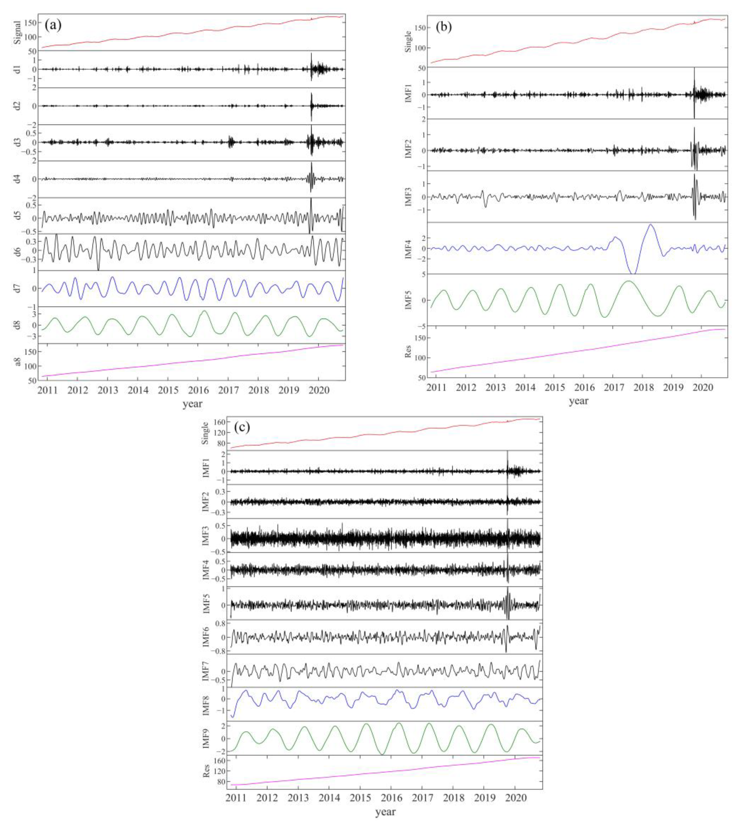
43]. The decomposed results of the denoised GNSS data via CEEMD in the N direction at station P242 are presented and compared with the properties of WD and EMD (Figure A2). d1–d6, d7–d8 and a8, which were extracted using WD, denote the noise, seasonal and trend terms, respectively (Figure A2a). IMF1–IMF3, IMF4–IMF5 and Res, which were extracted using EMD, denote the noise, seasonal and trend terms, respectively (Figure A2b). IMF1–IMF7, IMF8–IMF9, and Res extracted via CEEMD denote the noise, seasonal and trend terms, respectively (Figure A2c).
WD and EMD can be used to perform feature extraction on a time sequence. However, for WD, the amplitudes of the noise part are larger, which indicates that noise exerts a more significant effect on feature extraction. The EMD exhibits a modal overlap. To demonstrate the feature extraction ability of the CEEMD method, the similarity of the slope of the trend term and the Pearson correlation coefficients (PCCs) of the seasonal term were used for the denoised GNSS coordinate time series.
(1)
Comparison results between trend terms.
WD, EMD and CEEMD were applied to trend extraction for Blocks 1 and 2. The slopes of the original sequences and the trend terms were used to verify the superiority of the trend extraction. The similarity of the slope between the raw data and trend terms was calculated as follows:
S i m i l a r i t y = M s i O s i i = 1 , 2 , , u
where Similarity represents the similarity between trend terms, M s i represents the slope of the ith trend term and O s i represents the slope of the ith original data.
The similarity in the slope between the trend term and the denoised GNSS time series is presented in Table 4. The closer the trend term is to the slope value of the raw GNSS data, the more reliable is the extracted result. Based on Table 4, CEEMD is more stable and reliable than EMD and WD. The accuracy of CEEMD is 99.99%, which was higher than that of WD (99.96%) and EMD (97.60%), demonstrating that CEEMD is superior to WD and EMD in terms of trend-term extraction.
(2)
Comparison results between seasonal terms.
The performances of WD, EMD and CEEMD in extracting seasonal items were compared, and the PCC was used to establish the superiority of CEEMD (Table 5).
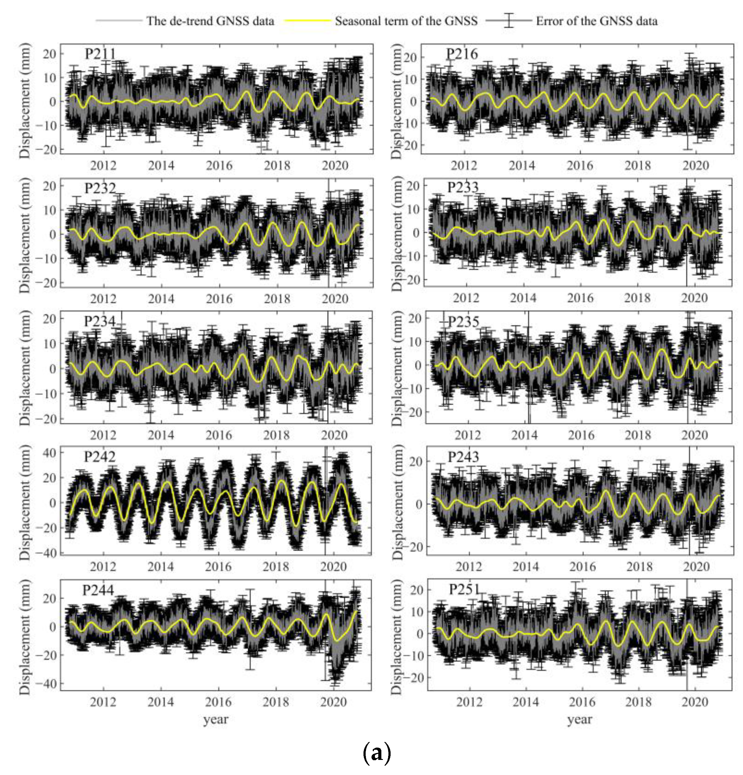
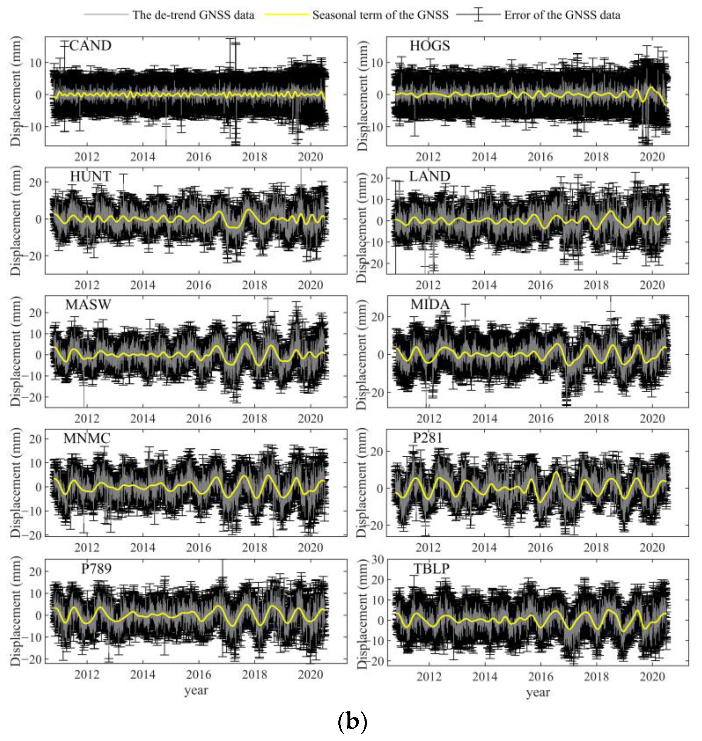
For Block 1, the average PCCs of the seasonal terms extracted via WD, EMD and CEEMD were 0.10, 0.18 and 0.35, respectively, whereas for Block 2, they were 0.12, 0.26 and 0.37, respectively (Table 5). The average PCCs obtained by CEEMD in Block 1 were 250.0% and 94.4% higher than those obtained by WD and EMD, respectively, whereas those in Block 2 were higher by 208.3% and 43.2%, respectively. These results demonstrate that CEEMD is more accurate than EMD and WD for the extraction of seasonal items. The seasonal terms extracted via CEEMD and the other parameters in Blocks 1 and 2 are shown in Figure 8a,b, respectively. Seasonal terms are indicated by yellow lines, GNSS detrended signals are illustrated by grey lines and the errors in GNSS data, which reflect the errors in GNSS signals, are represented by black I-shaped lines. The results showed that the seasonal terms extracted via CEEMD are consistent with the residual time series.

4.3. Noise Analysis

Typical methods for the noise characteristic analysis of GNSS data include maximum likelihood estimation (MLE) and power spectrum analysis. For noise analysis in a time sequence, the nature and intensity of noise in the GNSS data are determined in the frequency and time domains, respectively. Bos et al. [13] developed a technique that substantially increases the efficiency of the MLE method, which has since been improved [49]. Additionally, more advanced and computationally expensive methods, such as Markov chain Monte Carlo methods [14,50] and wavelet analysis [51], have been proposed to obtain unbiased probability distributions for noise in the time series. The definition of the related information criterion (IC) is provided in Appendix A.3.
He et al., objectively selected the best noise model by investigating various criteria such as the AIC and BIC [52]. The performance of the models investigated was quantified by analyzing 500 batches of simulated time series with lengths of 8.2, 16.4 and 24.6 years and known noise characteristics. He et al. processed a time series before jointly estimating stochastic and functional models using a maximum log-likelihood estimator via Hector software [13,53]. To prevent the over-selection of noise models with numerous parameters, the optimal noise model was selected based on the log-likelihood value and information criteria (i.e., AIC, BIC and BIC_tp). He et al., applied these information criteria to Monte Carlo simulations of synthetic time series and obtained highly reliable results [54]. In this study, the Hector software package was employed to estimate the parameters of various combinations of noise models, which were then used to analyze the noise in raw and denoised GNSS residual sequences at the selected GNSS sites in the two blocks. The AIC, BIC and BIC_tp were applied to describe the feasibility of each noise model. WN, WN plus PL noise (WN + PL), WN plus flicker noise (WN + FN), WN plus random walk noise (WN + RW), WN + FN + RW, generalized Gaussian–Markov noise (GGM) and WN plus generalized Gaussian–Markov noise (WN + GGM) were considered in the noise analysis.
The percentages of each noise model with the lowest AIC, BIC and BIC_tp values in the raw and denoised residual sequences of the selected GNSS stations (N, E and U) in Blocks 1 and 2 are shown in Table 6. The values of the AIC, BIC and BIC_tp were mostly consistent, thus demonstrating the reliability of the AIC, BIC and BIC_tp criteria used to determine the best noise model. Additionally, the optimal noise model for the raw GNSS residual sequence in the selected Blocks 1 and 2 regions can be regarded as a combination of the WN + FN + RW model with percentages of 46.7% and 46.7%, respectively, which is based on the BIC_tp criterion for the selection of the best noise model. Furthermore, the percentage of the WN + FN models was 26.7% in the Block 1 region, whereas that of the WN + PL model was 23.3% in the Block 2 region.
For the WD-PCA method for most cases in the selected Blocks 1 and 2 regions, a combination of GGM + WN can be regarded as the optimal noise model, followed by the GGM model. For the EMD-PCA method for most cases in the selected Blocks 1 and 2 regions, a combination of WN + FN + RW could be regarded as the optimal noise model, whereas the GCM model in Block 1 and WN + FN in Block 2 can be regarded as the second-most optimal model. For the proposed method, a combination of WN + GGM model can be regarded as the optimal noise model for most cases in the selected Blocks 1 and 2 networks, whereas the GGM model in Block 1 and GGM + WN model in Block 2 can be regarded as the second-best model. One can conclude that the noise components in the raw and denoised GNSS sequences are complex and that applying only one model to all the GNSS positions in the selected GNSS region is unreasonable (Table 6).
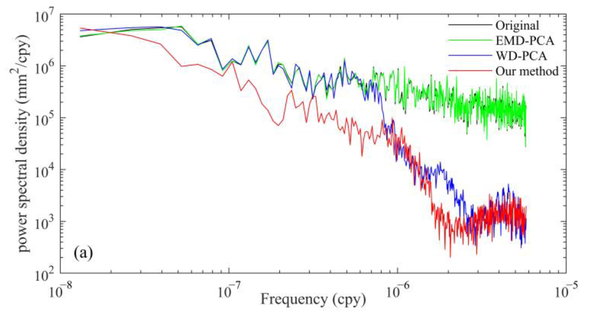
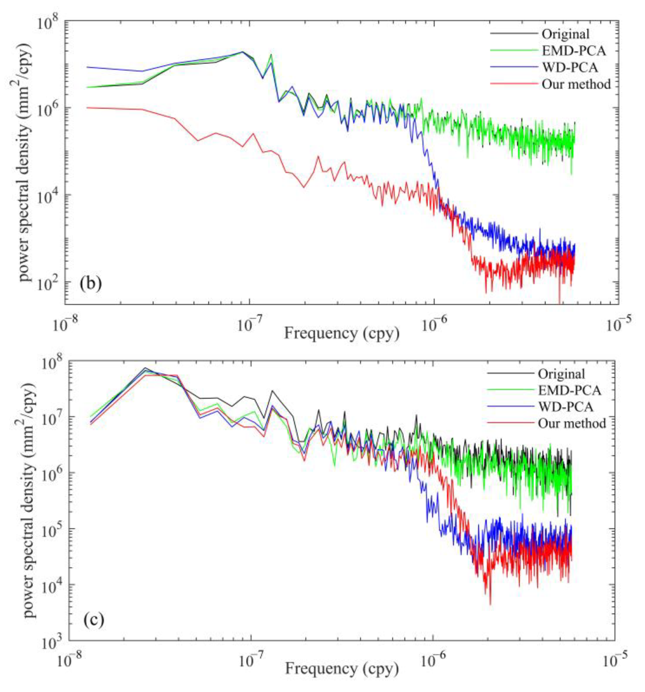
The power spectra of the raw and denoised GNSS residual sequences in the three directions at station P242 are shown in Figure A3. No significant period was removed by CEEMD, while WD-PCA and EMD-PCA eliminated high- and low-frequency noise, respectively; however, the clearance level was limited. The proposed method performed better than WD-PCA and EMD-PCA in eliminating low- and high-frequency noise, respectively. For high-frequency noise in the right side, both WD-PCA and the proposed method exhibited a favorable denoising effect, indicating that the two approaches can fully utilize the merits of the WD method for eliminating high-frequency noise. For the low-frequency noise in the intermediate section, the proposed method was significantly better than the other two methods for all three components. This indicates that the proposed method fully exploits the merits of CEEMD and WD, where CEEMD is first used to obtain various IMFs as well as because of its good adaptive processing ability by WD for noise-dominant IMFs. For the lower-frequency noise in the left side, the proposed method performed better than the other two methods, particularly for the horizontal components. This indicates that the proposed method fully considers the correlation between the different components of each station and the non-uniform behavior of the CME on a spatial scale.

5. Conclusions

To enhance the accuracy of GNSS positioning and feature extraction, an adaptive method using CEEMD and MPCA based on correlation coefficients and block spatial filtering was proposed. The proposed approach fully exploits the merits of CEEMD and WD to remove high- and low-frequency noise. Furthermore, the proposed method fully considers the correlation between the different components of each station and the non-uniform behavior of the CME on a spatial scale to eliminate low-frequency noise. Finally, the seasonal- and trend-term features of the denoised GNSS sequences were extracted using the CEEMD method. The properties of the proposed approach were estimated using a GNSS daily time series from two blocks in California, USA. The following four conclusions were drawn.
(1)
Compared with other typically applied approaches, the newly proposed approaches were more accurate in denoising the GNSS daily time series. In the Block 1 region in the N, E and U directions, the mean STDs of the raw residual data, WD-PCA and EMD-PCA were (1.15, 1.36, 5.70) mm, (0.57, 0.51, 4.32) mm and (0.76, 0.87, 4.59) mm, respectively, whereas those of the proposed approach were 0.27, 0.29 and 4.03 mm, respectively. In Block 2 in the N, E and U directions, the mean STDs of the raw residual data, WD-PCA and EMD-PCA were (1.09, 1.20, 4.79) mm, (0.28, 0.28, 3.19) mm and (0.50, 0.57, 3.58) mm, respectively, whereas those of the proposed approach were 0.15, 0.20 and 2.86 mm, respectively. The performance of the proposed approach across the two regions was consistent, indicating that it can effectively decrease noise at low- and high-frequency in GNSS daily sequences. The proposed method is suitable for denoising nonlinear and nonstationary GNSS position sequences.
(2)
WD, EMD and CEEMD were used to extract the features from the GNSS daily data. The results of the trend-feature extraction showed that the accuracy of CEEMD was 99.99% for trend-term feature extraction in the denoised GNSS daily sequences, which was higher than the 99.96% and 97.60% accuracy levels exhibited by WD for EMD, respectively. Compared with WD and EMD, CEEMD was more reliable and stable in Blocks 1 and 2. The results of seasonal-feature extraction demonstrated that the average PCC extracted via CEEMD was 0.36, which was 63.6% and 27.3% higher than those of WD and EMD, respectively. These results showed that the seasonal terms obtained by CEEMD were consistent with the residual time series, and that CEEMD is more reliable than WD and EMD.
(3)
For the raw GNSS data for most cases in Blocks 1 and 2, the WN + FN + RW model was the optimal noise model. For WD-PCA and EMD-PCA for most cases in Blocks 1 and 2, the WN + GGM and WN + FN + RW models were the best noise models. For the proposed method, the WN + GGM model was the best noise model in Blocks 1 and 2. The second-best model was the GGM model in Block 1 and the GGM + WN model in Block 2. These results were obtained possibly because the components of the noise in the raw and denoised GNSS data were complex, and that applying only one model to all the GNSS positions in the selected GNSS region is unreasonable.
(4)
Results of spectral analysis suggest that the proposed method is better than the other two methods for all three components. The proposed method is suitable for denoising nonlinear and nonstationary GNSS data. The advantage of the proposed method is that it fully exploits the merits of CEEMD and WD. CEEMD was first used to obtain various IMFs and then to obtain noise-dominant IMFs owing to its good adaptive processing ability. Finally, it fully considers the correlation between the different components of each station and the non-uniform behavior of the CME on a spatial scale.

Author Contributions

Conceptualization, Y.L.; methodology, Y.L.; validation, L.H.; formal analysis, L.H.; investigation, L.H.; data curation, L.H. and X.L.; writing—original draft preparation, L.H.; writing—review and editing, Y.L.; funding acquisition, Y.L. All authors have read and agreed to the published version of the manuscript.

Funding

This research was funded by the National Natural Science Foundation of China, grant number 41804001, Natural Science Foundation of Shandong Province, grant number ZR2019BD006. This research was also funded by Scientific Research Foundation of Shandong University of Science and Technology for Recruited Talents, under Grant number 2019RCJJ003.

Data Availability Statement

In view of confidentiality and the need for permission from the authors, data and materials will be available on request.

Acknowledgments

We thank the Scripps Orbit and Permanent Array Center (SOPAC), which provides the GNSS daily data available from SOPAC (http://sopac-ftp.ucsd.edu/pub/timeseries/measures/, accessed on 8 March 2023). Figures were generated using MATLAB software developed by the MathWorks, Inc., in Portola Valley, CA, USA.

Conflicts of Interest

No conflict of potential competing interest exits in the submission of this manuscript, and manuscript is approved by all authors for publication.

Appendix A

Appendix A.1. CEEMD Method

EMD is a signal decomposition method based on the adaptive decomposition of nonlinear and non-stationary data proposed by Huang, et al. [55]. For achieving signal decomposition, the traditional Fourier transform and wavelet transform project the signal to a pre-set function. In contrast, EMD without any predetermined basis function adaptively decomposes a time sequence into finite IMFs through continuous “screening” based on the inherent time-scale characteristics of a time sequence itself. Decomposed IMFs must meet two conditions: (i) the extreme number for one IMF is no more than one zero crossing number; (ii) the average value of the envelope determined by the minimum and maximum is zero [55]. For the given signal S ( t ) , the “screening” algorithm is used to obtain the first IMF step, as follows:
(1)
The locations of all the local minima and maxima in the signal S(t) are identified.
(2)
Interpolate a natural cubic spline through the local maxima (minima) to find the largest (smallest) envelope of S(t).
(3)
Calculate the mean values: a(t) = (max(t) + min(t))/2.
(4)
Remove details with: A(t) = S(t) − a(t).
(5)
Repeat steps (1) to (4) on d(t) until the stopping criterion is met; the resulting d(t) is referred to as an IMF, Ii(t).
(6)
Compute the residual with: R(t) = S(t) − Ii(t).
(7)
Iterate steps (1) to (6) until no more IMFs are available.
Here, the original datasets can be expressed as:
  S ( t ) = i = 1 n I i ( t ) + R n ( t )
where I i represents the ith IMF component, and n refers to the number of IMFs. R n ( t ) represents the final residue. The order of frequency for all decomposed IMFs is from high to low. IMFs can reveal the time series of the multi-scale turbulence characteristics of the residue.
In a multi-year position time series, IMF components with high frequency are generally deleted directly as noise, and the GNSS coordinate sequences can be denoised by the reconstruction of the remainder of IMFs [56,57]. Yet IMFs obtained by EMD usually exhibit mode mixing (noise and signal overlap), and the simple reconstruction of IMF components leads to poor denoising.
Based on the EMD method proposed by Huang, et al. [55], the ensemble empirical mode decomposition (EEMD) method was developed by adding white noise to the signal to reduce the mode mixing phenomenon of the EMD method. However, the EEMD method still has problems, including residual noise, unequal number of modes, large reconstruction error, and poor completeness of decomposition. Therefore, the complete ensemble empirical mode decomposition (CEEMD) method was developed by Yeh, et al. [58], where auxiliary white noise in pairs of negative and positive datasets is added to the raw dataset and can effectively improve the decomposition efficiency. Let the band decomposition signal be S(t) and let f(t) = S(t). The calculation procedures of the CEEMD algorithm are as below: In each stage of decomposition, a specific white noise is added, and a unique residual is calculated to obtain each IMF to complete the exact original signal reconstruction. The application results show that CEEMD is an effecient method in high-frequency denoising and low-frequency information extraction.
After signal decomposition using the CEEMD method, a series of IMFs ranked from high to low frequency can be obtained. During decomposition, remaining auxiliary noise in the dataset reconstruction can be eliminated effectively, which is advantageous in analyzing non-stationary and non-linear time sequence.

Appendix A.2. Correlation Coefficient between Each IMF and the Raw Signal

The IMFs obtained by CEEMD are arranged from high to low frequency according to signal attributes. IMFs with High frequencies primarily include random white noise, whereas IMFs with low frequencies typically include valid signals. Daniel [59] demonstrated that within the first several high-frequency IMF components, the principal function of white noise in each IMF gradually decreases, and the principal function of the signal gradually increases. Kaslovsky and Meyer [59] illustrated that the decomposed IMFs could be divided into three categories: (i) noise IMFs with white noise as the main component; (ii) transitional IMFs containing both noises and signals; and (iii) signal-dominant monochromatic IMFs.
The correlation coefficient (CC) between each IMF and the raw signal could be applied to fix the inflection point between the noise-controlled and signal-controlled IMFs. The CCs between each IMF and the raw signal can be defined as:
c c i , j ( X j , r i , j ) = m ( X i - X ¯ i ) ( r i , j - r ¯ i , j ) m ( X i - X ¯ i ) 2 m ( r i , j - r ¯ i , j ) 2
where X j is the jth signal, r i , j represents the ith IMF component of X j obtained by CEEMD, and m is the raw signal’s length.
According to the definition of transitional IMF by Li, et al. [60], the inflection point of the transitional IMF is as follows: from the first IMF, the IMF corresponding to the first extreme value of the CC is confirmed, and the latter is taken as the inflection point of transitional IMF.

Appendix A.3. Definition of IC

The definition of Akaike Information Criterion (AIC) is as below:
A I C = - 2 log ( L ) + 2 h
where L and h represent likelihood function and the number of model-fitting parameters [61], respectively.
The optimal model has the lowest AIC value and codes the most information with the smallest number of fitting parameters. AIC relative to h has a certain minimum value, and the model of appropriate order is determined by the value of h at the minimum. In general, when model complexity increases (h), L also increases so that the AIC declines. Yet, when the value of h is too large, the growth rate of the likelihood-function slows down, which leads to an increase in AIC, and overfitting occurs and the model becomes too complex. AIC can enhance model fitting and avoid overfitting. AIC has also been developed for other criteria, such as the Bayesian Information Criterion (BIC) [62], which contains a severe penalty by replacing 2h terms with h · ln ( u ) and introducing additional model parameters. When the sample sizes are considered, penalty term of the AIC will be smaller than that of BIC. When the samples sizes are too large, the complexity of the model resulted from high-accuracy can be effectively prevented.
The Bayesian modification of the AIC (BIC) is defined as:
B I C = h · log   ( u )   -   2 log   ( L )
where h and u represent the number of model fitting parameters and the samples, respectively, and L is the likelihood function.
In order to avoid the approximation of assuming that u is very large [63], Schwarz [64] reintroduced the original factor 2π into the derivation of the BIC, which we can call here BIC_tp:
B I C _ t p = - 2 log ( L ) + log ( u 2 π ) h

Appendix B

Figure A1. The effect of the developed denoising method in U direction for block 2. The grey lines denote original GNSS daily time series; the red lines denote the denoised GNSS daily time series; and the black I-shapes indicate errors with corresponding to GNSS positions.
Remotesensing 15 01902 g0a1
Figure A2. Decomposed results of the denoised GNSS data in N component at the P242 station based on WD (a), EMD (b), and CEEMD (c), respectively.
Remotesensing 15 01902 g0a2
Figure A3. Power spectral density of station ‘P242’ for North (a), East (b), and Up (c) directions, expressed in dB of mm2/cpy.
Remotesensing 15 01902 g0a3aRemotesensing 15 01902 g0a3b

References

  1. Parkinson, B.W.; Spilker, J.J. Progress in Astronautics and Aeronautics: Global Positioning System: Theory and Applications; AIAA: Reston, VA, USA, 1996; Volume 164. [Google Scholar]
  2. Hofmann-Wellenhof, B.; Lichtenegger, H.; Collins, J. Global Positioning System: Theory and Practice; Springer Science & Business Media: Berlin/Heidelberg, Germany, 2012. [Google Scholar]
  3. Bock, Y.; Melgar, D. Physical applications of GPS geodesy: A review. Rep. Prog. Phys. 2016, 79, 106801. [Google Scholar] [CrossRef]
  4. Blewitt, G.; Lavallée, D. Effect of annual signals on geodetic velocity. J. Geophys. Res. Solid Earth 2002, 107, ETG 9-1–ETG 9-11. [Google Scholar] [CrossRef] [Green Version]
  5. Li, S.-Q.; Chen, Q.-F.; Zhao, L.; Zhu, L.-P.; Gao, J.-Z.; Li, M.-F.; Liu, G.-P.; Wang, B. Anomalous focal mechanism of the May 2011 Mw 5.7 deep earthquake in Northeastern China: Regional waveform inversion and possible mechanism. Chin. J. Geophys. 2013, 56, 2959–2970. [Google Scholar] [CrossRef]
  6. Xiang, Y.; Yue, J.; Tang, K.; Li, Z. A comprehensive study of the 2016 Mw 6.0 Italy earthquake based on high-rate (10 Hz) GPS data. Adv. Space Res. 2019, 63, 103–117. [Google Scholar] [CrossRef]
  7. Xu, C.; Gong, Z.; Niu, J. Recent developments in seismological geodesy. Geod. Geodyn. 2016, 7, 157–164. [Google Scholar] [CrossRef]
  8. Amiri-Simkooei, A. On the nature of GPS draconitic year periodic pattern in multivariate position time series. J. Geophys. Res. Solid Earth 2013, 118, 2500–2511. [Google Scholar] [CrossRef] [Green Version]
  9. Wdowinski, S.; Bock, Y.; Zhang, J.; Fang, P.; Genrich, J. Southern California permanent GPS geodetic array: Spatial filtering of daily positions for estimating coseismic and postseismic displacements induced by the 1992 Landers earthquake. J. Geophys. Res. Solid Earth 1997, 102, 18057–18070. [Google Scholar] [CrossRef]
  10. Nikolaidis, R. Observation of Geodetic and Seismic Deformation with the Global Positioning System; University of California: San Diego, CA, USA, 2002. [Google Scholar]
  11. Dong, D.; Fang, P.; Bock, Y.; Webb, F.; Prawirodirdjo, L.; Kedar, S.; Jamason, P. Spatiotemporal filtering using principal component analysis and Karhunen-Loeve expansion approaches for regional GPS network analysis. J. Geophys. Res. Solid Earth 2006, 111, B03405. [Google Scholar] [CrossRef] [Green Version]
  12. He, X.; Hua, X.; Yu, K.; Xuan, W.; Lu, T.; Zhang, W.; Chen, X. Accuracy enhancement of GPS time series using principal component analysis and block spatial filtering. Adv. Space Res. 2015, 55, 1316–1327. [Google Scholar] [CrossRef]
  13. Bos, M.; Fernandes, R.; Williams, S.; Bastos, L. Fast error analysis of continuous GNSS observations with missing data. J. Geod. 2013, 87, 351–360. [Google Scholar] [CrossRef] [Green Version]
  14. Bos, M.S.; Montillet, J.-P.; Williams, S.D.P.; Fernandes, R.M.S. Introduction to Geodetic Time Series Analysis. In Geodetic Time Series Analysis in Earth Sciences; Montillet, J.-P., Bos, M.S., Eds.; Springer International Publishing: Cham, Switzerland, 2020; pp. 29–52. [Google Scholar]
  15. Santamaría-Gómez, A.; Bouin, M.N.; Collilieux, X.; Wöppelmann, G. Correlated errors in GPS position time series: Implications for velocity estimates. J. Geophys. Res. Solid Earth 2011, 116, 384–398. [Google Scholar] [CrossRef]
  16. Van Dam, T.; Wahr, J.; Milly, P.; Shmakin, A.; Blewitt, G.; Lavallée, D.; Larson, K. Crustal displacements due to continental water loading. Geophys. Res. Lett. 2001, 28, 651–654. [Google Scholar] [CrossRef] [Green Version]
  17. Dong, D.; Fang, P.; Bock, Y.; Cheng, M.; Miyazaki, S.I. Anatomy of apparent seasonal variations from GPS-derived site position time series. J. Geophys. Res. Solid Earth 2002, 107, ETG 9-1–ETG 9-16. [Google Scholar] [CrossRef] [Green Version]
  18. Penna, N.; Stewart, M. Aliased tidal signatures in continuous GPS height time series. Geophys. Res. Lett. 2003, 30, 2184. [Google Scholar] [CrossRef] [Green Version]
  19. Ray, J.; Altamimi, Z.; Collilieux, X.; Van Dam, T. Anomalous harmonics in the spectra of GPS position estimates. GPS Solut. 2008, 12, 55–64. [Google Scholar] [CrossRef]
  20. Ming, F.; Yang, Y.; Zeng, A.; Jing, Y. Analysis of seasonal signals and long-term trends in the height time series of IGS sites in China. Sci. China Earth Sci. 2016, 59, 1283–1291. [Google Scholar] [CrossRef]
  21. Yuan, L.G.; Ding, X.L.; Chen, W.; Kwok, S.; Chan, S.B.; Hung, P.S.; Chau, K.T. Characteristics of daily position time series from the Hong Kong GPS fiducial network. Chin. J. Geophys. 2008, 51, 976–990. [Google Scholar] [CrossRef]
  22. Jackson, D.A.; Chen, Y. Robust principal component analysis and outlier detection with ecological data. Env. Off. J. Int. Env. Soc. 2004, 15, 129–139. [Google Scholar] [CrossRef]
  23. Lu, C.-W.; Xia, F. Microseismic noise reduction based on EWT and Meyer adaptive threshold. Prog. Geophys. 2020, 35, 1010–1016. [Google Scholar] [CrossRef]
  24. Zeng, J.-W.; Han, L.-G.; Xu, Z. Virtual source signals de-noising based on wavelet transform. Prog. Geophys. 2018, 33, 2507–2511. [Google Scholar] [CrossRef]
  25. Mousavi, S.M.; Langston, C.A.; Horton, S.P. Automatic microseismic denoising and onset detection using the synchrosqueezed continuous wavelet transform. Geophysics 2016, 81, V341–V355. [Google Scholar] [CrossRef]
  26. Azarbad, M.R.; Mosavi, M. A new method to mitigate multipath error in single-frequency GPS receiver with wavelet transform. GPS Solut. 2014, 18, 189–198. [Google Scholar] [CrossRef]
  27. Bakshi, B.R. Multiscale PCA with application to multivariate statistical process monitoring. AIChE J. 1998, 44, 1596–1610. [Google Scholar] [CrossRef]
  28. Vautard, R.; Yiou, P.; Ghil, M. Singular-spectrum analysis: A toolkit for short, noisy chaotic signals. Phys. D Nonlinear Phenom. 1992, 58, 95–126. [Google Scholar] [CrossRef]
  29. Jia, R.-S.; Liang, Y.-Q.; Hua, Y.-C.; Sun, H.-M.; Xia, F.-F. Suppressing non-stationary random noise in microseismic data by using ensemble empirical mode decomposition and permutation entropy. J. Appl. Geophys. 2016, 133, 132–140. [Google Scholar] [CrossRef]
  30. Jin, T.; Xiao, M.; Jiang, W.; Shum, C.; Ding, H.; Kuo, C.Y.; Wan, J. An adaptive method for nonlinear sea level trend estimation by combining EMD and SSA. Earth Space Sci. 2021, 8, e2020EA001300. [Google Scholar] [CrossRef]
  31. Kong, Q.; Zhang, L.; Han, L.; Guo, J.; Zhang, D.; Fang, W. Analysis of 25 years of polar motion derived from the DORIS space geodetic technique using FFT and SSA methods. Sensors 2020, 20, 2823. [Google Scholar] [CrossRef]
  32. Shen, Y.; Zheng, W.; Yin, W.; Xu, A.; Zhu, H. Feature extraction algorithm using a correlation coefficient combined with the VMD and its application to the GPS and GRACE. IEEE Access 2021, 9, 17507–17519. [Google Scholar] [CrossRef]
  33. Xu, H.; Lu, T.; Montillet, J.-P.; He, X. An improved adaptive IVMD-WPT-Based noise reduction algorithm on GPS height time series. Sensors 2021, 21, 8295. [Google Scholar] [CrossRef]
  34. Montillet, J.-P.; Tregoning, P.; McClusky, S.; Yu, K. Extracting white noise statistics in GPS coordinate time series. IEEE Geosci. Remote Sens. Lett. 2012, 10, 563–567. [Google Scholar] [CrossRef]
  35. Lu, C.; Kuang, C.; Zhang, H.; Yi, Z. Multipath correction method by combining EMD and PCA. Geotech. Investig. Surv. 2014, 42, 58–62. [Google Scholar]
  36. He, X.; Yu, K.; Montillet, J.-P.; Xiong, C.; Lu, T.; Zhou, S.; Ma, X.; Cui, H.; Ming, F. GNSS-TS-NRS: An Open-source MATLAB-Based GNSS time series noise reduction software. Remote Sens. 2020, 12, 3532. [Google Scholar] [CrossRef]
  37. Lee, T.; Ouarda, T.B. An EMD and PCA hybrid approach for separating noise from signal, and signal in climate change detection. Int. J. Climatol. 2012, 32, 624–634. [Google Scholar] [CrossRef]
  38. Zhang, H.; Kuang, C.; Lu, C.; Zhou, Y. A multipath correction method based on wavelet filtering and PCA. J. Geod. and Geodynamics 2013, 33, 137–141. [Google Scholar] [CrossRef]
  39. Lu, J.; Chen, X.; Feng, S. A GPS Time Series Prediction Model Based on CEEMD. J. Adv. Comput. Netw 2016, 4, 70–74. [Google Scholar] [CrossRef] [Green Version]
  40. Zhao, L.; Gao, J.; Li, Z.; Wang, J. GPS Multipath Correction Algorithm Based on CEEMD-Wavelet-SavGol Model. Bull. Surv. Mapp. 2017, 11, 1. [Google Scholar] [CrossRef]
  41. Li, Y.; Han, L.; Yi, L.; Zhong, S.; Chen, C. Feature extraction and improved denoising method for nonlinear and nonstationary high-rate GNSS coseismic displacements applied to earthquake focal mechanism inversion of the El Mayor-Cucapah earthquake. Adv. Space Res. 2021, 68, 3971–3991. [Google Scholar] [CrossRef]
  42. Tregoning, P.; Watson, C. Atmospheric effects and spurious signals in GPS analyses. J. Geophys. Res. Solid Earth 2009, 114, 1–15. [Google Scholar] [CrossRef] [Green Version]
  43. Wu, Z.; Huang, N.E.; Long, S.R.; Peng, C.-K. On the trend, detrending, and variability of nonlinear and nonstationary time series. Proc. Natl. Acad. Sci. USA 2007, 104, 14889–14894. [Google Scholar] [CrossRef] [Green Version]
  44. Jiang, W.-P.; Li, Z.; Liu, H.-F.; Zhao, Q. Cause analysis of the non-linear variation of the IGS reference station coordinate time series inside China. Chin. J. Geophys. 2013, 56, 2228–2237. [Google Scholar] [CrossRef]
  45. Tian, Y.; Shen, Z. Progress on reduction of non-tectonic noise in GPS position time series. Acta Seismol. Sin. 2009, 31, 68–81. [Google Scholar]
  46. Goudarzi, M.A.; Cocard, M.; Santerre, R.; Woldai, T. GPS interactive time series analysis software. GPS Solut. 2013, 17, 595–603. [Google Scholar] [CrossRef]
  47. Bogusz, J.; Klos, A. On the significance of periodic signals in noise analysis of GPS station coordinates time series. GPS Solut. 2016, 20, 655–664. [Google Scholar] [CrossRef] [Green Version]
  48. Blewitt, G. Self-consistency in reference frames, geocenter definition, and surface loading of the solid Earth. J. Geophys. Res. Solid Earth 2003, 108. [Google Scholar] [CrossRef] [Green Version]
  49. Langbein, J. Improved efficiency of maximum likelihood analysis of time series with temporally correlated errors. J. Geod. 2017, 91, 985–994. [Google Scholar] [CrossRef] [Green Version]
  50. Olivares-Pulido, G.; Teferle, F.N.; Hunegnaw, A. Markov chain Monte Carlo and the application to geodetic time series analysis. In Geodetic Time Series Analysis in Earth Sciences; Montillet, J.-P., Bos, M.S., Eds.; Springer International Publishing: Cham, Switzerland, 2020; pp. 53–138. [Google Scholar]
  51. Kaczmarek, A.; Kontny, B. Identification of the noise model in the time series of GNSS stations coordinates using wavelet analysis. Remote Sens. 2018, 10, 1611. [Google Scholar] [CrossRef] [Green Version]
  52. He, X.; Bos, M.S.; Montillet, J.P.; Fernandes, R.M.S. Investigation of the noise properties at low frequencies in long GNSS time series. J. Geod. 2019, 93, 1271–1282. [Google Scholar] [CrossRef]
  53. He, X.; Montillet, J.-P.; Fernandes, R.; Melbourne, T.I.; Jiang, W.; Huang, Z. Sea Level Rise Estimation on the Pacific Coast from Southern California to Vancouver Island. Remote Sens. 2022, 14, 4339. [Google Scholar] [CrossRef]
  54. He, X.; Bos, M.S.; Montillet, J.-P.; Fernandes, R.; Melbourne, T.; Jiang, W.; Li, W. Spatial variations of stochastic noise properties in GPS time series. Remote Sens. 2021, 13, 4534. [Google Scholar] [CrossRef]
  55. Huang, N.E.; Shen, Z.; Long, S.R.; Wu, M.C.; Shih, H.H.; Zheng, Q.; Yen, N.-C.; Tung, C.C.; Liu, H.H. The empirical mode decomposition and the Hilbert spectrum for nonlinear and non-stationary time series analysis. Proc. R. Soc. Lond. Ser. A Math. Phys. Eng. Sci. 1998, 454, 903–995. [Google Scholar] [CrossRef]
  56. Boudraa, A.; Cexus, J.; Saidi, Z. EMD-based signal noise reduction. Int. J. Signal Process. 2004, 1, 33–37. [Google Scholar] [CrossRef]
  57. Yang, G.; Liu, Y.; Wang, Y.; Zhu, Z. EMD interval thresholding denoising based on similarity measure to select relevant modes. Signal Process. 2015, 109, 95–109. [Google Scholar] [CrossRef]
  58. Yeh, J.-R.; Shieh, J.-S.; Huang, N.E. Complementary ensemble empirical mode decomposition: A novel noise enhanced data analysis method. Adv. Adapt. Data Anal. 2010, 2, 135–156. [Google Scholar] [CrossRef]
  59. Kaslovsky, D.N.; Meyer, F.G. Noise corruption of empirical mode decomposition and its effect on instantaneous frequency. Adv. Adapt. Data Anal. 2010, 2, 373–396. [Google Scholar] [CrossRef] [Green Version]
  60. Li, Y.; Xu, C.; Yi, L.; Fang, R.J.J.o.G. A data-driven approach for denoising GNSS position time series. J. Geod. 2018, 92, 905–922. [Google Scholar] [CrossRef]
  61. Akaike, H. A new look at the statistical model identification. IEEE Trans. Autom. Control. 1974, 19, 716–723. [Google Scholar] [CrossRef]
  62. Schwarz, G. Estimating the dimension of a model. Ann. Stat. 1978, 6, 461–464. [Google Scholar] [CrossRef]
  63. Anderson, D.; Burnham, K. Model Selection and Multi-Model Inference; Springer: Berlin/Heidelberg, Germany, 2004; Volume 63, p. 10. [Google Scholar]
  64. Schwarz, G.J.T. Estimating the Dimension of a Model. 1978, pp. 461–464. Available online: https://www.jstor.org/stable/2958889 (accessed on 8 March 2023).
Figure 1. Distribution of International GNSS Service (IGS) reference stations.
Remotesensing 15 01902 g001
Figure 2. (a) Raw coordinate time series of P242 station, and (b) the corresponding residual time series.
Remotesensing 15 01902 g002
Figure 3. Flowchart of the proposed method.
Remotesensing 15 01902 g003
Figure 4. Decomposed results based on the CEEMD method in N direction of GNSS station P242.
Remotesensing 15 01902 g004
Figure 5. (a) Raw and denoised GNSS coordinate time series in N direction of site P242, and (b) their corresponding residual time series. (Black lines: raw time series; green lines: resuls via WD-PCA; blue lines: resuls via EMD-PCA; red lines: resuls via the propsed method).
Remotesensing 15 01902 g005
Figure 6. Effect of the proposed denoising method in U direction for Block 1. Grey lines denote original GNSS daily time series; red lines denote denoised GNSS daily time series; and black I-shapes indicate errors corresponding to GNSS positions.
Remotesensing 15 01902 g006
Figure 7. Standard deviations of raw and denoised GNSS residual data in three directions for Blocks 1 and 2.
Remotesensing 15 01902 g007
Figure 8. Extraction effect of GNSS seasonal term (yellow lines) in N direction based on CEEMD for Block 1 (a), and Block 2 (b). Grey lines denote de-trended GNSS sequence, and black I-shapes indicate errors corresponding to GNSS sequence.
Remotesensing 15 01902 g008aRemotesensing 15 01902 g008b
Table 1. Data loss rates for Blocks 1 and 2.
Block 1Data Loss Rate (%)Block 2Data Loss Rate (%)
P2111.23CAND3.49
P2161.78HOGS0.63
P2321.33HUNT1.31
P2331.25LAND1.23
P2340.46MASW0.5
P2350.85MIDA1.46
P2420.68MNMC2.73
P2430.59P2811.82
P2440.77P7891.01
P2510.83TBLP3.95
Table 2. CCs between each component location in site P242 based on the position time series and its corresponding IMFs.
IMFc1c2c3c4c5c6c7c8
N0.410.370.320.290.320.410.760.51
Table 3. Average standard deviations of raw and denoised residual data (mm).
MethodsOverall DenoisingBlock 1Block 2
NEUNEUNEU
Original1.121.285.251.151.365.71.091.24.79
WD-PCA0.450.533.70.570.514.320.280.283.19
EMD-PCA0.560.683.910.760.874.590.50.573.58
Our method0.310.33.460.270.294.030.150.22.86
Table 4. Similarity between denoised GNSS time series and trend term obtained via WD, EMD and CEEMD, separately.
Block 1Similar degree (%)Block 2Similar Degree (%)
WDEMDCEEMDWDEMDCEEMD
P21199.9799.9199.99CAND99.9799.9499.97
P21699.9999.6599.98HOGS99.9599.9999.99
P23299.9999.8999.99HUNT99.9599.9699.99
P23399.9699.8999.98LAND99.9699.9799.99
P23499.9799.9999.99MASW99.9799.9599.99
P23599.97100100MIDA99.9810099.99
P24299.8999.9999.98MNMC99.9399.9699.97
P24399.9699.9899.99P28199.9799.4299.99
P24499.9353.6599.97P78999.9599.91100
P25199.9599.97100TBLP99.9599.899.96
Table 5. Similarity of seasonal terms based on WD, EMD and CEEMD.
Block 1PCCsBlock 2PCCs
WDEMDCEEMDWDEMDCEEMD
P2110.010.050.39CAND0.020.20.31
P2160.120.210.31HOGS0.010.350.4
P2320.010.030.37HUNT0.010.060.39
P2330.130.340.31LAND0.020.360.4
P2340.010.060.37MASW0.130.350.42
P2350.010.30.36MIDA0.120.230.35
P2420.130.380.36MNMC0.010.350.34
P2430.120.220.32P2810.290.050.4
P2440.310.10.34P7890.290.230.32
P2510.130.150.32TBLP0.280.370.38
Table 6. Percentage of each noise model with the lowest values of the Akaike information criterion (AIC), Bayesian information criterion (BIC) and BIC_tp of the raw and denoised GNSS residual sequences at Blocks 1 and 2 (the value in bold indicates the optimal noise model (%)).
BlockNoise ModelRawWD-PCAEMD-PCAOur Method
AICBICBIC_tpAICBICBIC_tpAICBICBIC_tpAICBICBIC_tp
1WN000000000000
WN + PL0010000000000
WN + FN23.33026.700023.336.73.3000
WN + FN + RW43.336.746.700046.733.353.3000
WN + RW06.76.703.33.33.313.32013.33013.3
GGM23.326.71036.74020101003.33046.7
WN + GGM100063.356.776.716.76.723.383.34040
2WN000000000000
WN + PL23.31023.3000000000
WN + FN1026.72000006.76.7000
WN + FN + RW6046.746.70007046.73.3000
WN + RW06.7003.33.36.723.301016.713.3
GGM3.3106.72026.733.30053.346.746.723.3
WN + GGM3.303.3807063.323.323.336.743.336.763.3
Disclaimer/Publisher’s Note: The statements, opinions and data contained in all publications are solely those of the individual author(s) and contributor(s) and not of MDPI and/or the editor(s). MDPI and/or the editor(s) disclaim responsibility for any injury to people or property resulting from any ideas, methods, instructions or products referred to in the content.

