Article

Accuracy Assessment and Impact Factor Analysis of GEDI Leaf Area Index Product in Temperate Forest

1
Engineering Research Center of Ministry of Education for Mine Ecological Restoration, China University of Mining and Technology, Xuzhou 221116, China
2
School of Environment Science and Spatial Informatics, China University of Mining and Technology, Xuzhou 221116, China
3
Geospatial Sciences Center of Excellence, South Dakota State University, 1021 Medary Ave, Wecota Hall Box 506B, Brookings, SD 57007, USA
4
State Key Laboratory of Remote Sensing Science, Jointly Sponsored by Beijing Normal University and Institute of Remote Sensing and Digital Earth of Chinese Academy of Sciences, Beijing 100875, China
5
Beijing Engineering Research Center for Global Land Remote Sensing Products, Institute of Remote Sensing Science and Engineering, Faculty of Geographical Science, Beijing Normal University, Beijing 100875, China
*
Author to whom correspondence should be addressed.
These authors contributed equally to this work.
Remote Sens. 2023, 15(6), 1535; https://doi.org/10.3390/rs15061535
Submission received: 8 February 2023 / Revised: 7 March 2023 / Accepted: 9 March 2023 / Published: 10 March 2023
(This article belongs to the Special Issue Application of LiDAR Point Cloud in Forest Structure)

Abstract

:
The leaf area index (LAI) is a vital parameter for quantifying the material and energy exchange between terrestrial ecosystems and the atmosphere. The Global Ecosystem Dynamics Investigation (GEDI), with its mission to produce a near-global map of forest structure, provides a product of the effective leaf area index (referred to as GEDI LAIe). However, it is unclear about the performance of GEDI LAIe across different temperate forest types and the degree of factors influencing GEDI LAIe performance. This study assessed the accuracy of GEDI LAIe in temperate forests and quantifies the effects of various factors, such as the difference of gap fraction (DGF) between GEDI and discrete point cloud Lidar of the National Ecological Observatory Network (NEON), sensor system parameters, and characteristics of the canopy, topography, and soil. The reference data for the LAIe assessment were derived from the NEON discrete point cloud Lidar, referred to as NEON Lidar LAIe, covering 12 forest types across 22 sites in the Continental United States (the CONUS). Results showed that GEDI underestimated LAIe (Bias: −0.56 m2/m2), with values of the mean absolute error (MAE), root mean square error (RMSE), percent bias (%Bias), and percent RMSE (%RMSE) of 0.70 m2/m2, 0.89 m2/m2, −0.20, and 0.31, respectively. Among forest types, the underestimation of GEDI LAIe in broadleaf forests and mixed forests was generally greater than that in coniferous forests, which showed a moderate error (%RMSE: 0.33~0.52). Factor analysis indicated that multiple factors explained 52% variance of the GEDI LAIe error, among which the DGF contributed the most with a relative importance of 49.82%, followed by characteristics of canopy and soil with a relative importance of 23.20% and 16.18%, respectively. The DGF was a key pivot for GEDI LAIe error; that is, other factors indirectly influence the GEDI LAIe error by affecting the DGF first. Our findings demonstrated that the GEDI LAIe product has good performance, and the factor analysis is expected to shed some light on further improvements in GEDI LAIe estimation.

Graphical Abstract

1. Introduction

Leaf area index (LAI) is defined as half of the total leaf area per unit of the ground surface area [1]. Being a direct proxy of leaves, LAI plays an irreplaceable role in studies of surface thermal radiation, nitrogen deposition, fire monitoring, wildlife protection, and carbon sequestration in terrestrial ecosystems [2,3,4,5]. LAI can be precisely measured directly from destructive sampling of vegetation or indirectly estimated from collected optical images, such as the Digital Hemispherical Photography (DHP) images, based on the Beer–Lambert Law (Beer’s law) in quadrat sampling [6]. The LAI collected by the above two field-measured approaches is usually used for validating LAI products [7,8,9]. However, field surveys consume time, cost, and labor, which hinders their application over a large area. In contrast, indirect methods based on remote sensing data are promising because of the various available datasets for LAI measurement over local, regional, or even global scales [10]. Active remote sensing, especially Lidar, is broadly recognized as an excellent source for LAI measurement owing to its ability to measure leaf area density from the top canopy to the forest floor directly [11,12]. Lidar is also more sensitive to LAI than passive optical images which suffer from spectral saturation [11,12], e.g., Landsat LAI is saturated when LAI is greater than 5 m2/m2 [12].
Spaceborne Lidar is an ideal source for LAI estimation over a large-scale area, due to its ideal cost and acceptable acquisition frequency for sampling [13,14,15]. Currently, three free open accessed spaceborne Lidar are available, including the first and second generation of Ice, Cloud, and land Elevation Satellite (namely ICESat-1 and ICESat-2) and the global ecosystem dynamics investigation (GEDI), in which the effectiveness using ICESat-1 and ICESat-2 for LAI estimation has been demonstrated [14,16]. GEDI, as the second generation full-waveform Lidar after ICESat-1, has several improvements [15], including: (1) a higher sampling frequency with 4-day revisit; (2) a denser coverage (51.6°S~51.6°N), especially for temperate and tropical areas with a footprint distance of 600 m across orbit and 60 m along orbit; and (3) a smaller diameter of footprint (25 m), which can alleviate the influence of topographic slope [17,18]. These improvements are expected to be a step forward for an accurate estimation of LAI [19,20].
Tang et al. (2019) [21] used the Geometric Optical Radiative Transfer (GORT) [22] to invert the gap fraction for producing a near-global effective leaf area index (LAIe) product with GEDI, referred to as GEDI LAIe. At present, few researchers have assessed the accuracy of the GEDI LAIe product [19,20]. For example, Dhargay et al. (2022) evaluated the accuracy of GEDI LAIe over a temperate forest in south-eastern Australia taking Airborne Laser Scanning (ALS) Lidar collected in 2016 as a reference [20]. Ilangakoon et al. (2021) used ALS Lidar acquired in 2014 to assess the GEDI LAIe accuracy across savanna forests in a semi-arid area [19]. However, limited forest types and outdated reference data used in these previous researches might provide only limited insight into GEDI LAIe performance across diverse forest types [19,20]. Since a comprehensive assessment of the GEDI performance of LAIe estimation is a prerequisite for its appropriate application [23,24,25,26], it is urgent to conduct an evaluation of GEDI LAIe over various geographic units and forest types.
To effectively interpret the performance of GEDI LAIe, it is necessary to employ reliable and higher-resolution observations that cover various forest ecosystems. The datasets of the National Ecological Observatory Network (NEON) can be regarded as an ideal evaluation reference. NEON provides exciting nationwide, coordinated, multitemporal, and high-quality LiDAR and field survey data collected at 81 sites across 21 eco-climate domains spanning 30 years from the Airborne Observation Platform (AOP) and Terrestrial Observation System (TOS) [27,28,29]. The advantages of wide distribution and consistency of NEON’s AOP and TOS observations make their datasets valuable for the assessment and cross-site comparison of satellite products. For example, Wang et al. (2021) [30] and Liu et al. (2020) [31] evaluated GEDI products of canopy height and ground elevation using NEON AOP datasets across the USA. Kang et al. (2021) validated the LAI product of Landsat with NEON TOS DHP data [32].
Theoretically, GEDI LAIe is influenced by factors [13,16,18] including GEDI sensor parameters, characteristics of canopy and soil, and topographic slope [19,20,33,34,35]. For example, the signal-to-noise ratio and the transmitted pulse energy are important parameters of the GEDI sensor [20,30] which directly impact GEDI waveform quality [15]. The physical and chemical characteristics of the canopy and soil within a footprint affect the shape and intensity of the GEDI waveform because a waveform intensity of specific height is proportional to the intersecting surface, direction, and reflectance of objects at the corresponding height [36,37]. Topographic slope not only directly increases the terrain but also indirectly affects waveform intensity through a complicated interaction with other factors such as canopy reflectance [30]. Additionally, the GEDI LAIe product was generated under the hypothesis of a random spatial distribution of foliage which might obey the fact of heterogeneous distribution of leaves. Thus, GEDI LAIe should be adjusted by dividing the clumping index which represents the degree of non-random distribution against the random distribution of leaves over space [2,8,38,39,40,41]. Previous studies have reported an underestimation of true LAI (LAIt) without the adjustment for LAIe [39].
The objectives of this study are (1) evaluating the accuracy of GEDI LAIe across various forest types and NEON sites and (2) quantifying the magnitude and direction of factors affecting GEDI LAIe estimation. This study evaluated the accuracy of GEDI LAIe and factors influencing GEDI LAIe performance by employing field-measured datasets from the Fenghuang Mountains in China and the LAIe estimated from discrete point cloud Lidar of NEON AOP, referred to as NEON Lidar LAIe, covering 12 forest types and spanning various geographic area across the Continental United States (CONUS).
To the best of our knowledge, this is the first study to systematically assess the performance of GEDI LAIe and quantify the importance and direct and indirect impact of various factors spanning various geographic units, and abundant forest types in various eco-climate regions. The accuracy assessment of GEDI LAIe among various geographic sites and forest types can answer if the GEDI LAIe product meets a specific requirement of ecological models, estimates of forest health and functioning, and biodiversity monitoring. The findings of factors influencing the performance of GEDI LAIe are expected to provide insight to enable proposal of better filters to screen footprint data for a better application, improve inversion methods for LAI estimation, and modify sensor parameters for next-generation spaceborne Lidar.

2. Materials and Methods
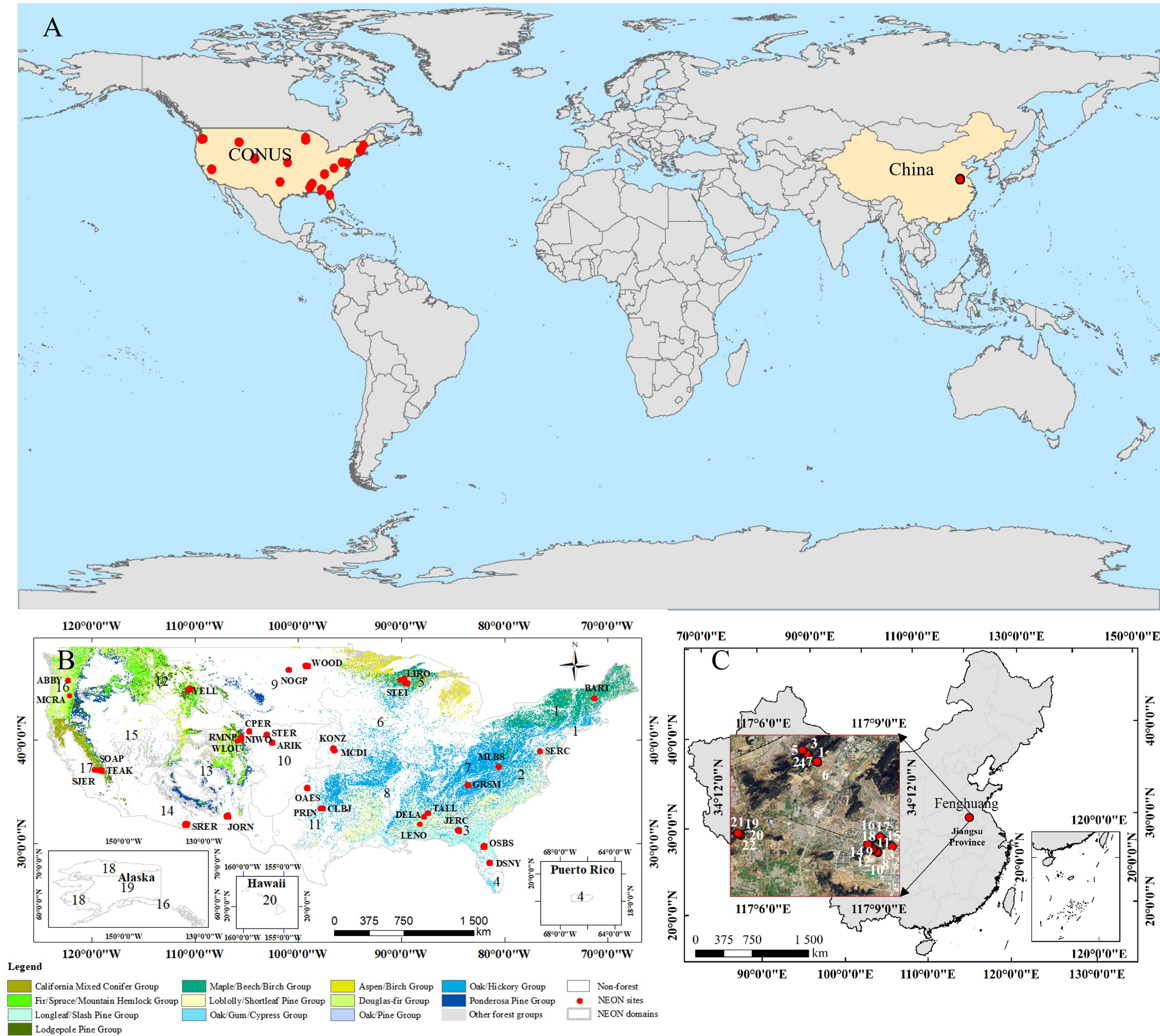
2.1. Study Areas

The CONUS (−124°44′4.59″~−66°53′30.90″W, 24°32′33.17″~49°22′10.17″N) and Fenghuang Mountains in Xuzhou City, Jiangsu Province, China (117°05′3.68″–117°10′24.13″E, 34°09′57.46″–34°13′38.76″N) were selected as the study areas (Figure 1). The reference datasets of NEON Lidar LAIe are environmentally distributed over the CONUS, which spans 17 eco-climatic geographic units and contains rich forest types (coniferous, broadleaf, mixed, etc.). Details of the NEON sites are shown in Supplementary Table S1. Forest types can be found in [30].
The Fenghuang Mountains are in Xuzhou City, Jiangsu Province, China. The 22 plots of field-measured LAIe in the Fenghuang Mountains belong to the temperate monsoon climate, with an average annual temperature of 14.9°, an average annual rainfall of 800~930 mm, and an altitude of less than 237 m. The tree species are mainly Platycladus orientalis, with a small number of Firmiana platanifolia, Broussonetia papyrifera, Ligustrum lucidum, Melia azedarach, Celtis bungeana, and Pistacia chinensis Bunge. The mean tree height of the 22 footprints ranges from 3.9 to 9.8 m; the mean DBH is less than 10 cm; and the tree density is greater than 900 trees/hm2.

2.2. Datasets and Preprocessing

2.2.1. GEDI Data

Since February 2019, NASA’s Distributed Archive of Land Surface Processes (LP DAAC) has released GEDI L1B (geolocated waveform), GEDI L2A (product of canopy height), GEDI L2B (product of foliage characteristics), and GEDI04_A and GEDI04_B (biomass products) [15]. For evaluation of GEDI LAIe performance, the GEDI L1B and GEDI L2B collected during 2019–2021 over the NEON sites across the CONUS were downloaded from the LP DAAC. For comparison of LAIe between GEDI and field measurements in Fenghuang Mountains, two available GEDI L2B orbits including GEDI02_B_2021105070412_O13253_03_T07142_02_003_01_V002 and GEDI02_B_2019159 105633_O02758_03_T01450_02_003_01_V002 were also downloaded from LP DAAC.
To select high-quality GEDI L2B data for GEDI LAIe accuracy analysis, the l2a_quality_flag and l2b_quality_flag equal to 1, degrade_flag equal to 0, landsat_water_persistence of less than 10%, urban_proportion equal to 0, and leaf_off_flag equal to 0 were used to selected good quality GEDI shots that were observations without orbit degradation, did not cover permanent water and urban areas, and were collected in the vegetation growing season [26,30,42]. To further remove outliers, GEDI shots with a difference of less than 50 m between the GEDI ground elevation and the elevation of the TanDEM-X Digital Elevation Model (DEM) were selected [30]. To select forested shots, the filters for landsat_treecover greater than 0, modis_treecover greater than 0, and vegetation height greater than 5 m were used [43].
Notably, GEDI products have a geolocation error of 10.2 m (1σ) [44]. To narrow the discrepancy between GEDI and NEON Lidar caused by this geolocation error, waveform matching was used to identify the GEDI footprint geolocation that best matched the NEON Lidar simulated waveform [45]. The NEON Lidar simulated waveforms were calculated within a 10 × 10 m range of provided GEDI geolocation in 1 m steps. The method of waveform simulation of NEON Lidar, as well as the parameter setup, is described in [45,46].

2.2.2. NEON Data

NEON simultaneously provides datasets collected from the Terrestrial Observation System (TOS) and the Airborne Observation Platform (AOP) [27,28]. The TOS aims at field monitoring of forest structures in plots, while the mission of AOP is to collect high-resolution and accurate airborne remote sensing data. NEON Lidar is one of the AOP products used for evaluating the performance of GEDI LAIe. To quantify the uncertainty of NEON Lidar LAIe, DHP images collected from the NEON TOS plots were used to calculate a field measure of LAIe. The NEON AOP’s DEM and NEON individual tree products were used to extract the topographic slope and tree distribution characteristics within each footprint.
NEON Lidar (accessed on 25 December 2022) [47], TOS DHP images (accessed on 31 January 2023) [48], and DEM (accessed on 25 December 2022) [49] were downloaded from the NEON Scientific Data Center (https://data.neonscience.org/data-products/explore), while the individual tree product [50,51,52] is available at https://zenodo.org/record/3765872# YzZ YC9hByUk (accessed on 20 September 2022). Details of the NEON Lidar, TOS field observations, and the individual tree product are as follows:
(1) NEON Lidar
The NEON Lidar was collected in the peak greenness of growing seasons from 2017 to 2019 (Supplementary Table S1), which is preprocessed with the step of denoise, point cloud classification, and high normalization.
(2) NEON DHP images
NEON TOS provides the DHP images collected in the plot of the flux tower (20 × 20 m). Each plot collects 12 DHP images with 4 m intervals from directions of east, west, south, and north (Supplementary Figure S1). A 180-degree 16 mm Nikon full-frame fisheye lens mounted on a full-frame Nikon DSLR camera was used for the DHP collection. Each NEON site with upward DHP images greater than the number of 12 was used for DHP LAIe estimation. The NEON DHP images, collected from July to September 2019 with an image size of 7360 × 4912, were processed by the software CAN_EYE V6.495 developed by the Emmah laboratory of the French agricultural research institute. The processes of DHP images included optical center selection and projection, gamma correction, masking, automated binary classification, and estimation of LAIe and LAIt [53]. The method of LAIe estimation in the CAN_EYE V6.495 depends on a look-up table for zenithal variation of theoretical gap fraction [54]. By segmenting each DHP into interest segments by angular of zenith and azimuth, DHP LAIe can be estimated by minimizing a cost function of the difference between measured and look-up-table gap fraction [55]. For stable estimation, the Lang graphical method was employed in this study, in which the resolutions of both zenith and azimuth for segmenting imagery were set to 5.0° [56].
(3) NEON individual tree products
NEON individual tree product provides the location, crown area, and height of each tree. The first three terms are derived from NEON’s high-resolution RGB images using the DeepForest method, while the tree height of each tree was extracted from NEON CHM [50,51,52]. Based on this product, we calculated the tree density in each footprint (i.e., the number of trees), the mean crown area of trees, the mean height of trees (tree height), the standard deviation of the crown area, and the standard deviation of tree height for the analysis of the effect factors.

2.2.3. DHP Images Collected in Fenghuang Mountains

This study collected field-measured LAIe derived from DHP across the 22 plots in the Fenghuang Mountains collected during 7–10 August 2022 (Supplementary Table S2). The plots were designed with a size of 40 × 40 m corresponding to each GEDI footprint. Notably, the second GEDI product has a 10.2 m geolocation uncertainty [44]. To alleviate the influence of the geolocation uncertainty on the comparison of LAIe between GEDI and field plots, the plots of neighboring buildings, roads, and escarpment were screened out. Considering GEDI LAIe in Fenghuang Mountains was collected in early growing seasons differing from the peak greenness of growing seasons for the field survey, plots covered with deciduous forest were carefully filtered out. As a result, a total of 13 plots were employed for validating the performance of GEDI LAIe. In each plot, a total of 24 DHP images were collected with a 15 mm Nikon Fisheye Lens mounted on a full-frame Canon Mark III camera in 4 perpendicular directions. To be consistent with the design of the field survey for the DHP collection of NEON TOS, this paper selected the nearest 12 DHP images from the plot center for DHP LAIe estimation. The same as the process of NEON DHP, these collected DHP images were then used to calculate DHP LAIe and LAIt using the software CAN_EYE V6.495 (see details in Section 2.2.2).

2.2.4. Forest Type Inventory

To explore the variation of GEDI LAIe accuracy across different forest types, we refer to the 250 m resolution forest type inventory produced by the USDA Forest Service–Forest Inventory and Analysis (FIA) Program and Remote Sensing Applications Center (RSAC) [57], downloaded from https://www.fs.usda.gov/research/inventory/FIA (accessed on 15 April 2020). A total of 12 forest types over the CONUS were selected, including seven coniferous forests, one mixed forest, and four broadleaf forests. These forest types cover 82.5% of the forested areas of the CONUS, with different conditions of tree height, canopy cover, vertical layer, and topography.

2.2.5. Soil Data

The organic matter content (SOC), soil nitrogen content (N), and soil pH from a depth of 0–5 cm were extracted from the Soilgrids data (https://soilgrids.org/ (accessed on 10 November 2022)), which is a global 3D soil raster product with a spatial resolution of 250 m [58]. The above three soil attributes were used as factors influencing GEDI LAIe.

2.2.6. Vegetation Cover

For canopy clumping correction of GEDI LAIe, the vegetation cover was calculated from the normalized difference vegetation index (NDVI) based on the principle of pixel dichotomy model, in which the NDVI derived from the Level 1T (L1T) image of Landsat 8 OLI covering the Fenghuang Mountains collected on 5 June 2021 (image ID of LC081210362021060502T1) was download from the USGS Earth Resources Observation and Science (EROS) Center.

2.3. Analysis Strategies

2.3.1. GEDI LAIe Estimation Method

GEDI LAIe is estimated from a gap fraction (P) based on Beer’s law formulated as a logarithmic function form (1). The gap fraction regarded as the complement of the canopy cover can be inverted by GORT using a ground-to-total energy ratio (2):
L A I e = 1 G × Ω × I n ( P )  
P = 1 1 1 + R g R v × ρ v ρ g
where G is the leaf projection distribution function with its default setting of 0.5 (spherical distribution), Ω is the clumping index with a default setting of 1, R g / R v is the ground-to-total energy ratio, and the ρ v / ρ g is the ratio of vegetation and soil reflectance.

2.3.2. NEON Lidar LAIe Estimation Method

Based on Beer’s Law, NEON Lidar LAIe can be estimated using (1). Differing from the ground-to-total energy ratio of waveform Lidar, the Lidar Penetration Index (LPI) is generally used as a proxy of the gap fraction estimation for LAIe estimation using discrete point cloud Lidar. Methods for estimating LPI include intensity-based, count-based, and voxel-based methods [59]. The intensity-based method is sensitive to the reflectance of vegetation and land surface [11], while the voxel-based method is controversial because of its unclear physical meaning [54,60]. The count-based method, which uses the ratio of ground returns to all returns for LPI estimation (3) is the most mature and easiest to interpret. Thus, the count-based method was used in this study to estimate the LPI:
L P I = N g N a l l
where N g is the number of returns for ground, N a l l   is the number of all returns. To alleviate the impact from the understory, LiDAR returns above 2 m were used for canopy LPI estimation [61].

2.3.3. Accuracy Assessment Strategy

The field-measured LAIe collected in the Fenghuang Mountains and the NEON Lidar LAIe were employed to verify the accuracy of GEDI LAIe, while the accuracy of NEON Lidar LAIe was verified by filed LAIe derived from NEON TOS’s DHP images. The bias, mean absolute error (MAE), root mean square error (RMSE), percent bias (%Bias), and percent RMSE (%RMSE) were used as accuracy indicators. To analyze the GEDI LAIe performance over different geographic units and forest types, accuracy comparisons of GEDI LAIe were conducted over the 22 NEON sites and the 12 forest types across the CONUS. The calculation of bias, MAE, RMSE, %Bias, and %RMSE can be found in [30].

2.3.4. Effects of Factor analysis Strategy

According to Beer’s law, the gap fraction is a key input for the LAIe estimation. Thus, the error of gap fraction estimation can directly convert to LAIe [22]. Given that, the difference of gap fraction between GEDI and NEON Lidar (DGF) can be an indicator to explain the difference of LAIe between GEDI and NEON Lidar. Meanwhile, the GEDI LAIe product uses the GORT for gap fraction estimation [21]. The performance of the GORT is influenced by characteristics of canopy and soil, which are correlated to input parameters of R g / R v and ρ v / ρ g in GORT [22]. In addition to factors, including DGF, and characteristics of the canopy and soil, which are directly related to GEDI LAIe estimation based on GORT, factors of sensor system parameters were selected to reflect the quality of GEDI observation and the reliability of NEON Lidar being taken as the reference. The consideration of NEON Lidar quality can help to explore the influence degree of the reference data quality on the GEDI LAIe assessment. Meanwhile, the characteristics of the topographic slope were taken into account for their effect on GEDI data quality. For example, a steep slope complicates the GEDI waveform by mixing up the reflectance energy of the canopy and ground [17]. As such, a total of 19 factors, categorized into DGF, characteristics of canopy and soil, sensor system parameters, and characteristics of the topographic slope, were employed to explain the error in GEDI LAIe estimation (Table 1).
To quantify the influence degree of each factor, we calculated the relative importance of each effect factor to the absolute deviation of GEDI LAIe using the LMG function in the “relaimpo” R package. LMG decomposes the variance of the dependent variable into non-negative single-factor variance contributions without being affected by the covariance among independent variables. The ratio of decomposed variance contribution to the variance of the dependent variable represents the relative importance [62].
To analyze the diverse direct and indirect effects of factors on the absolute deviation of GEDI LAIe, a structural equation model was built using IBM® SPSS® Amos. The structural equation model formulates a series of path relationships between independent variables (i.e., the nine factors) and dependent variables (i.e., absolute deviation of GEDI04_A), namely the indirect effect of “independent variable–independent variable–, …, –dependent variable” and the direct effect of “independent variable–dependent variable” [63,64]. The path relationship was quantified using linear regression models. The χ 2 , χ 2 /df, Goodness-of-Fit Index (GFI), Adjusted Goodness-of-Fit Index (AGFI), and Root Mean Square Error of Approximation (RMSEA) were used to determine the validity of the formulated structural equation model.

2.3.5. Leaves Clumping Analysis Strategy

GEDI LAIe was estimated based on the GORT. The GORT assumes that leaves are randomly distributed within the GEDI footprint (i.e., Beer–Lambert law), which disregards the fact that leaves clump at different scales including footprint, crown, branch, and cluster [65]. As a result, a difference occurs between GEDI LAIe and LAIt. The difference between GEDI LAIe and LAIt can be corrected by using the clumping index ( Ω ), namely, the ratio of LAIe to LAIt [6,33,66,67]. Commonly, the clumping index ranges from 0 to 1, with smaller values representing a higher level of clumping [33]. To quantify the impact of clumping, this study used (4) to express the relative errors of GEDI LAIe based on the clumping index.
e = Ω 1
The vegetation clumping within the footprint ( Ω footprint ) consists of the between-crown clumping ( Ω cover ) and within-crown clumping ( Ω crown ) [33]. The between-crown clumping shows the aggregation degree of crowns, which represents the laser that directly reaches the ground without interaction with any crown [66,67]. The within-crown clumping refers to a degree of the non-uniform length of laser transmission crowns against the uniform length assumed by the Beer–Lambert law [66]. We defined Ω footprint , Ω cover , and Ω crown using (5)–(7) to quantify the relative errors caused by the clumping effect of footprint, between-crown clumping, and within-crown clumping, respectively.
Ω footprint = LAI e / LAI t
Ω cover = LAI e / LAI cover
Ω crown = LAI cover / LAI t
where LAIe is GEDI LAIe, LAI t is derived from DHP images collected in the Fenghuang Mountains, and the LAI cover is the corrected result of between-crown clumping [59], calculated by:
LAI cover = 1 G × cover × I n ( P 1 + cover cover )
where G is set as 0.5 assuming that G obeys spherical distribution, and the cover is the vegetation cover calculated from the Landsat image.

3. Results

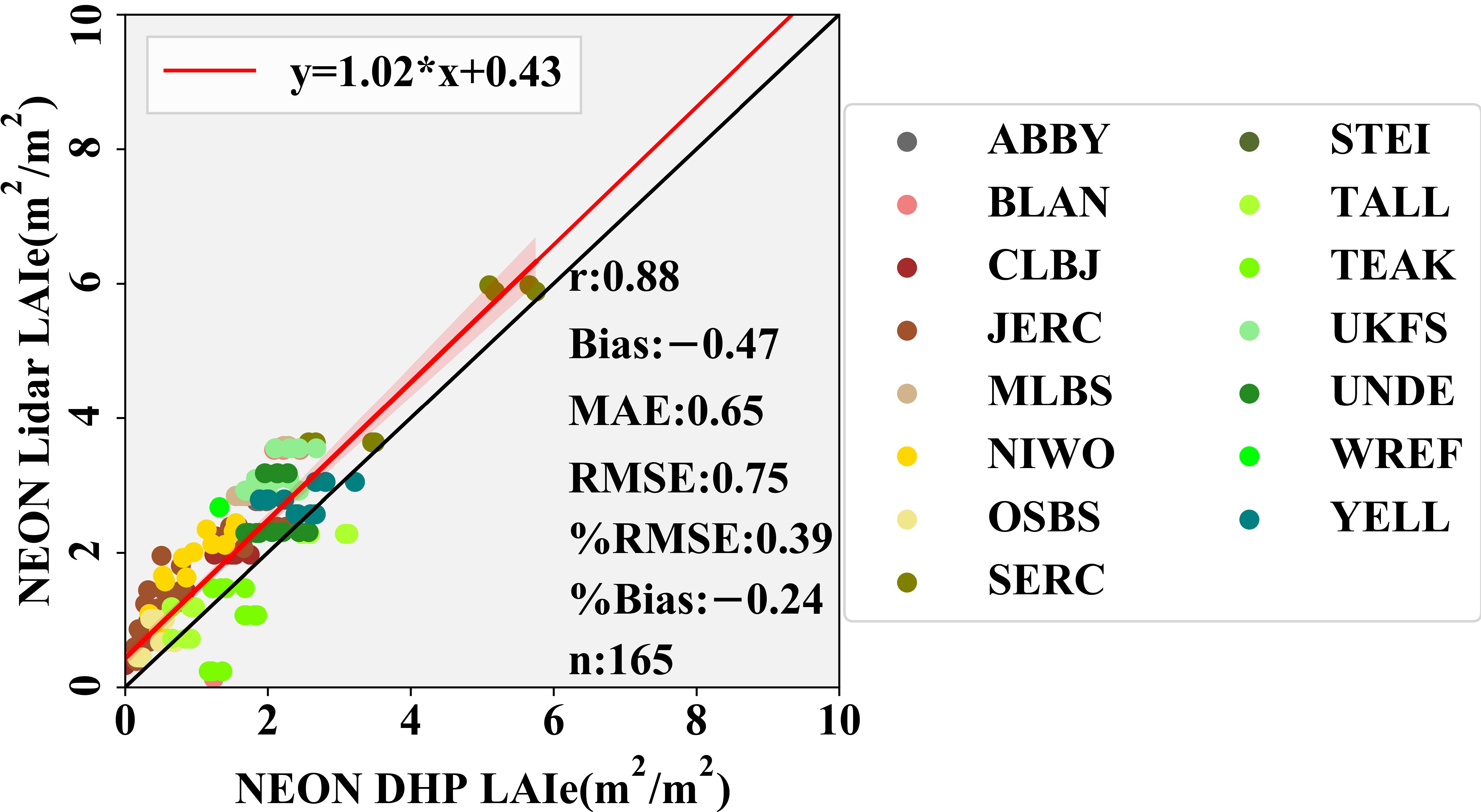
3.1. Accuracy of NEON Lidar LAIe

The accuracy of NEON Lidar LAIe was evaluated using the NEON DHP LAIe (Figure 2). Results show that the NEON Lidar LAIe and NEON DHP LAIe were significantly correlated, with an r value of 0.88 (p < 0.05). The bias value of −0.47 m2/m2 indicates that NEON Lidar overestimated LAIe with the MAE and RMSE values of 0.65 m2/m2 and 0.75 m2/m2, respectively. The %Bias and %RMSE, with values of −0.24 and 0.39, respectively, indicate a moderate error of NEON Lidar LAIe compared to NEON DHP LAIe. The scatters were distributed along the 1:1 line, which demonstrates the consistency of LAIe between NEON Lidar and NEON DHP images. Given the high correlation and reasonable error of NEON Lidar LAIe, it is suitable and reliable to use NEON Lidar LAIe as a reference for evaluating GEDI LAIe.

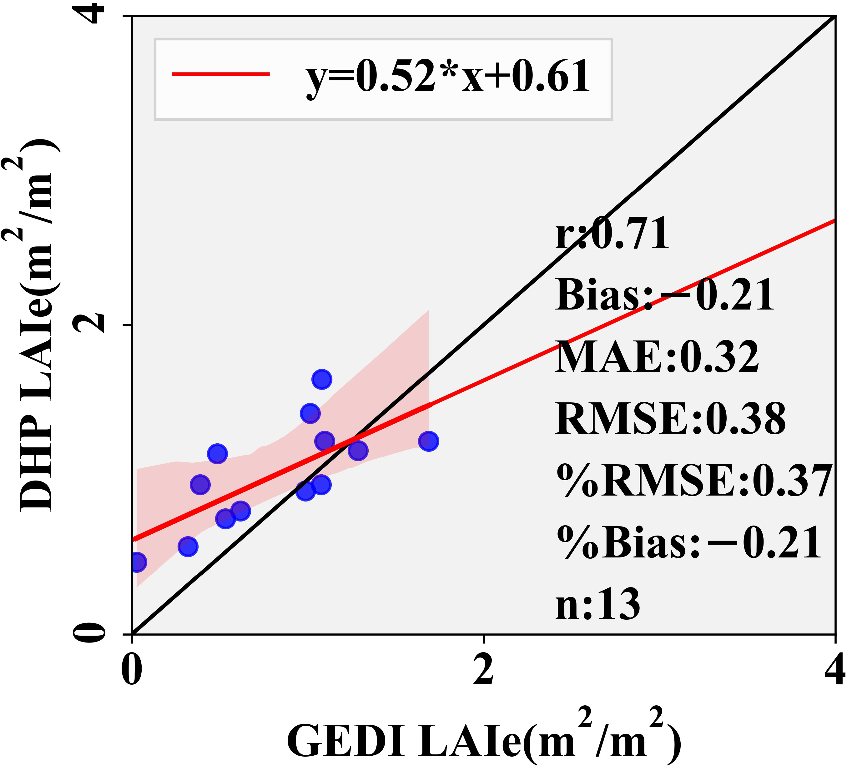
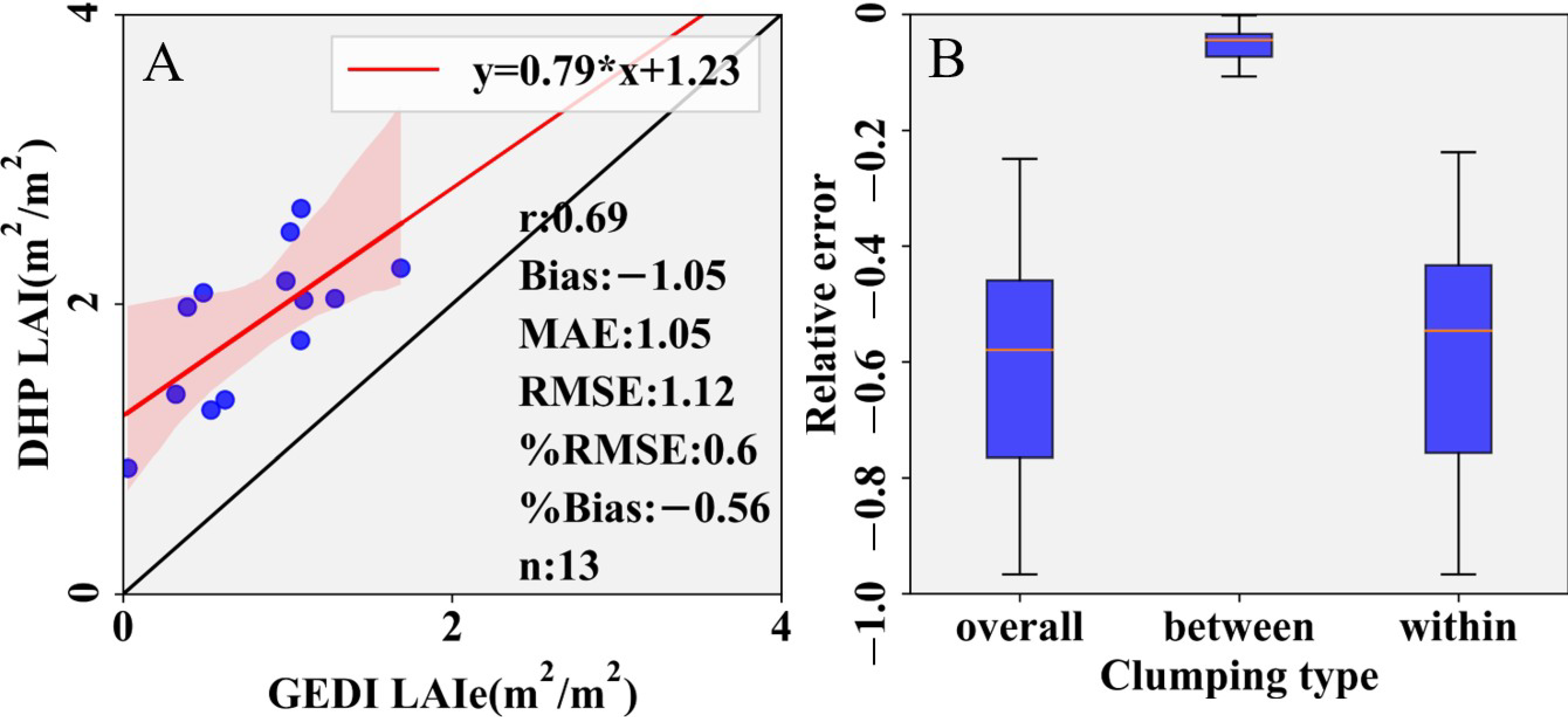
3.2. Comparison of LAIe between GEDI and Field Measurements

A total of 13 high-quality plots with field-measured DHP LAIe in the Fenghuang Mountains were used to estimate the accuracy of GEDI LAIe (Figure 3). Results show a high correlation between GEDI LAIe and DHP LAIe (r value of 0.71). The bias value of −0.21 m2/m2 shows that GEDI underestimated LAIe with MAE and RMSE values of 0.32 m2/m2 and 0.38 m2/m2. The %Bias and %RMSE values of −0.21 and 0.37, respectively, indicate a medium error of GEDI LAIe compared to field measurements. The scatter plot shows that the underestimation is more serious for GEDI observations with LAIe less than 1 m2/m2.

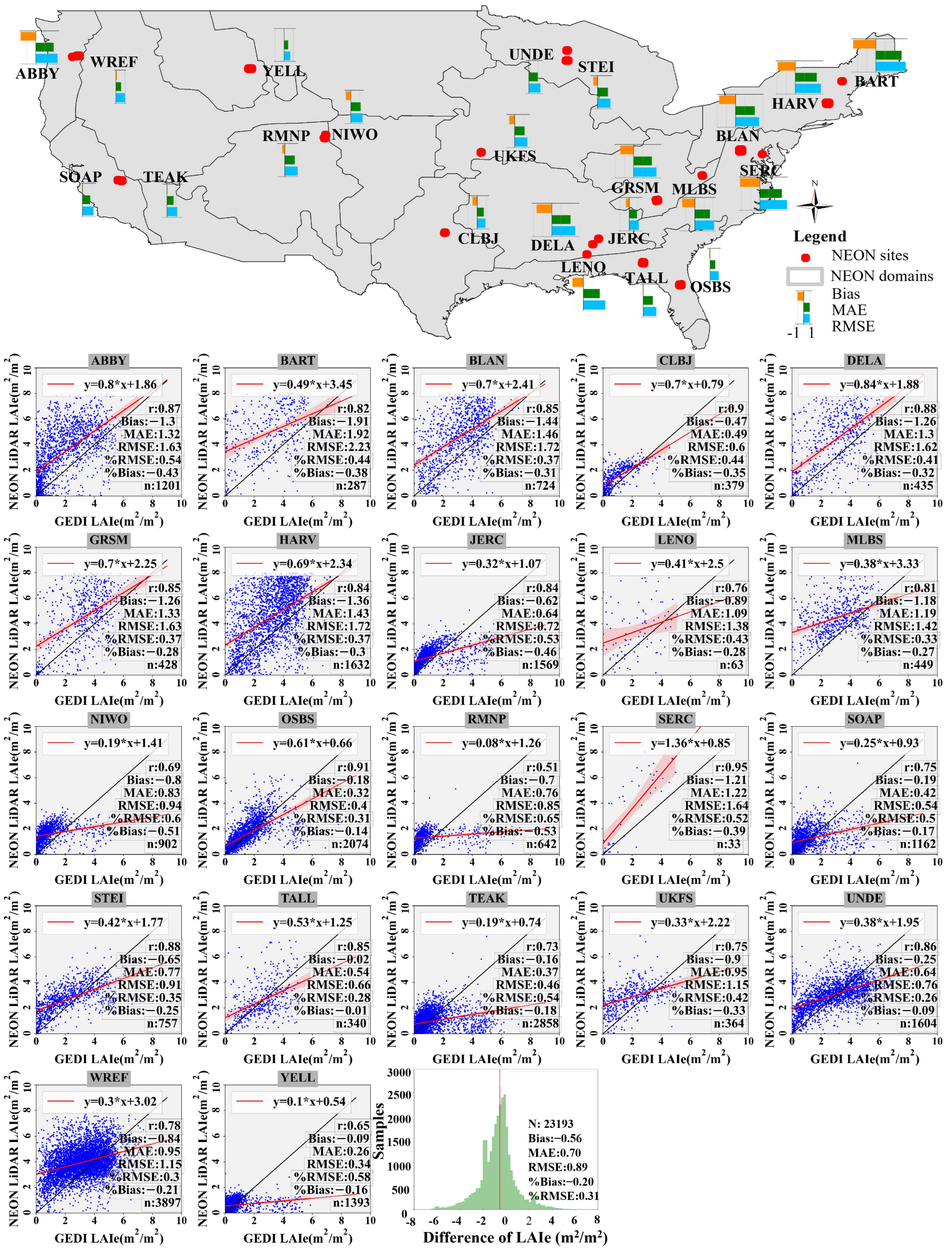
3.3. Accuracy of GEDI LAIe at Different NEON Sites

The accuracy of GEDI LAIe across the 22 sites taking NEON Lidar LAIe as reference datasets was estimated (Figure 4). The values of bias, MAE, RMSE, %Bias, and %RMSE (1σ) were −0.56 m2/m2, 0.70 m2/m2, 0.89 m2/m2, −0.20, and 0.31, respectively. The negative bias indicates the underestimation of GEDI LAIe compared to NEON Lidar LAIe. Meanwhile, the values of %Bias and %RMSE show a moderate error in GEDI LAIe.
The accuracy of GEDI LAIe among different sites showed a significant correlation between GEDI LAIe and NEON Lidar LAIe (r > 0.5, p < 0.05). Among the 22 NEON sites, the values of bias, MAE, and RMSE ranged from −1.91 to −0.02 m2/m2, from 0.26 m2/m2 to 1.92 m2/m2, and from 0.34 m2/m2 to 2.23 m2/m2. The accuracy variation of GEDI LAIe over the CONUS showed that the sites with the higher error were mostly distributed in the eastern (such as BART, HARV, BLAN, SERC, and MLBS) and western (e.g., ABBY) forests compared to the sites located in central regions of the CONUS.
Comparison of %RMSE values among NEON sites showed that it was a challenge for GEDI to precisely estimate LAIe, especially in dense and heterogeneous forests. Specifically, 3 out of 22 sites had a low relative error (%RMSE less than 0.3), 12 out of 22 sites had a moderate relative error (%RMSE greater than 0.3 but less than 0.5), and 7 out of 22 sites had a high relative error (%RMSE greater than 0.5). Among these sites with a high relative error, the sites of ABBY, TEAK, and SERC are covered with dense forests in the western and eastern CONUS [57], and the sites of JERC, NIWO, RMNP, and YELL are covered with sparse forests in a high-heterogeneity landscape in the central CONUS [57].

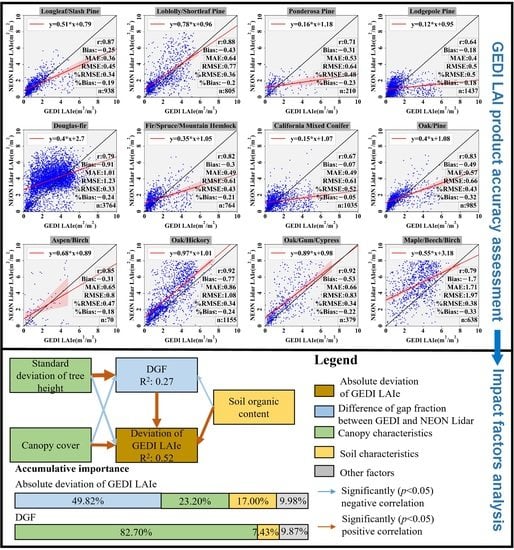
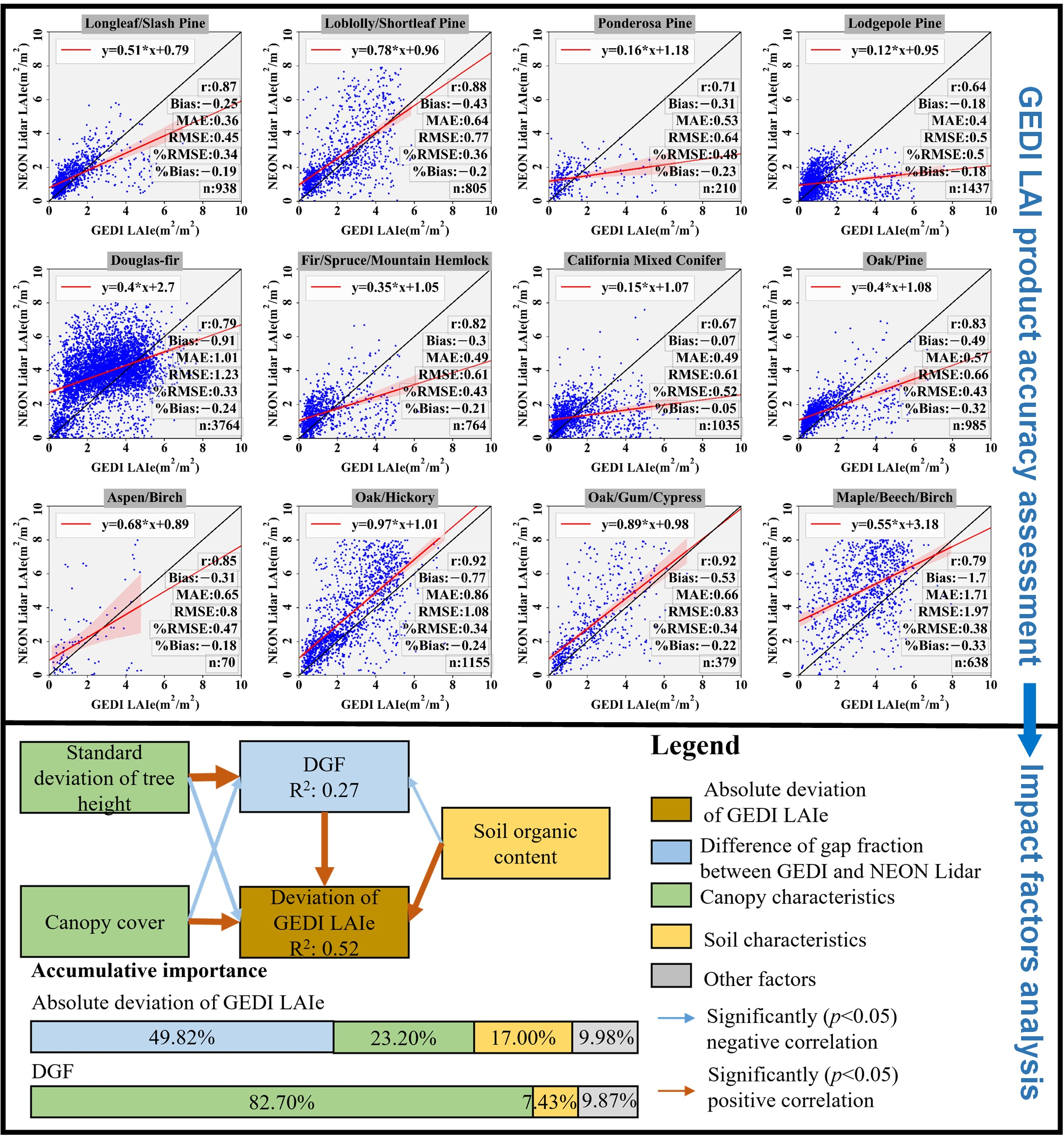
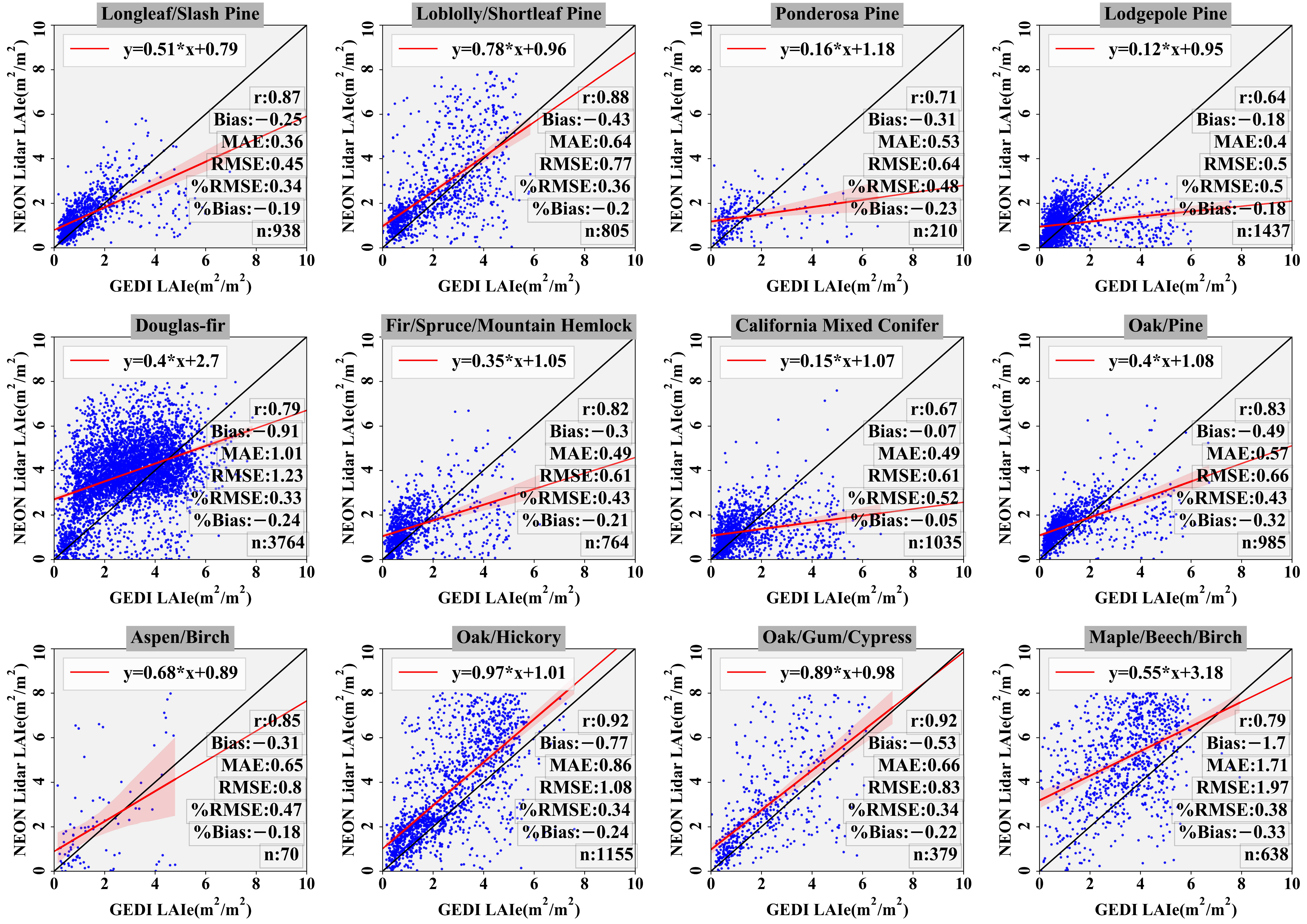
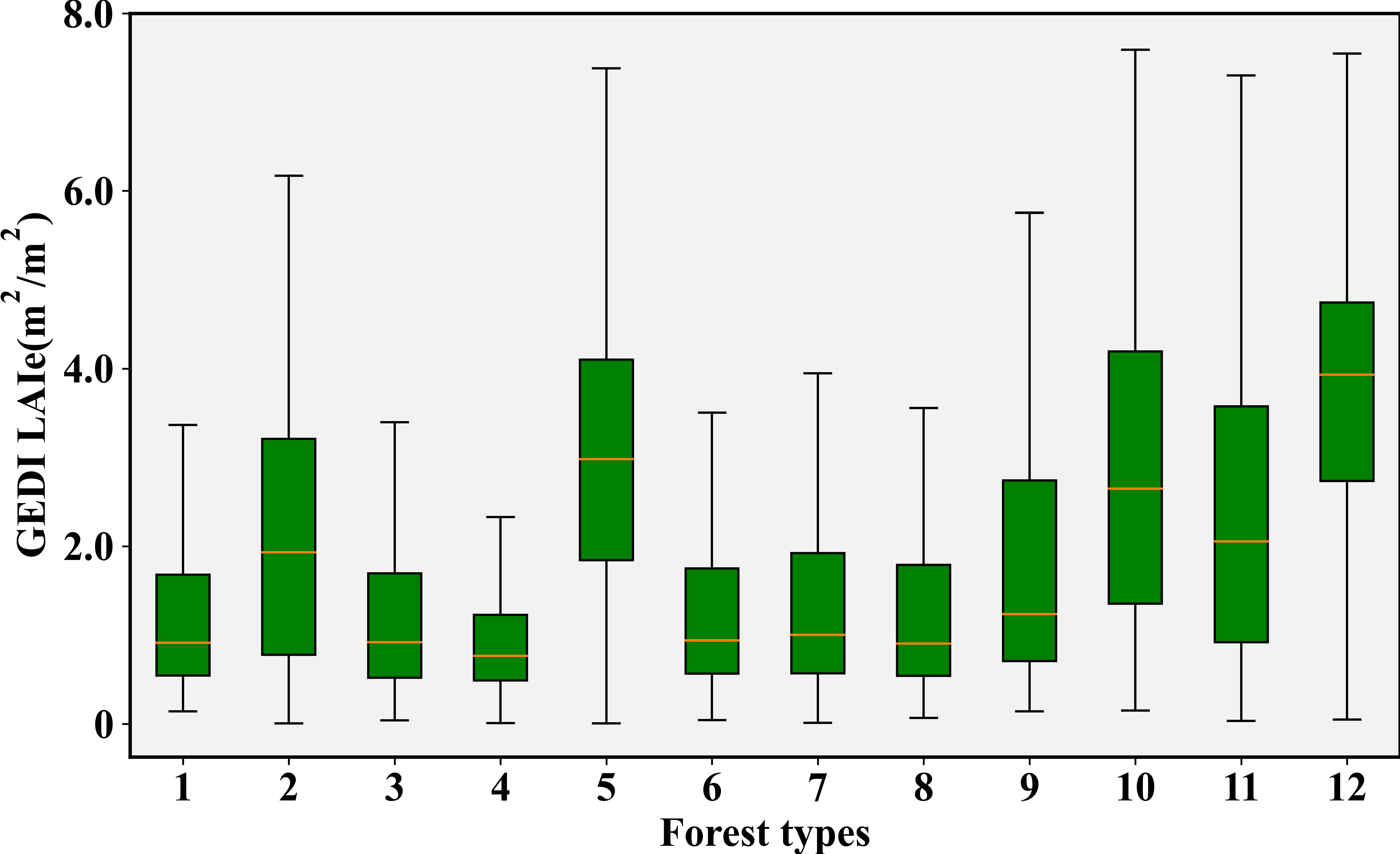
3.4. Accuracy GEDI LAIe among Forest Types

The performance of GEDI LAIe estimation was analyzed among the 12 temperate forest types across the CONUS, including seven types of coniferous forest, one type of mixed forest, and four types of broadleaf forest (Figure 5 and Figure 6). Results showed a significant correlation between GEDI LAIe and NEON Lidar LAIe (r > 0.6, p < 0.05) with a great variation in accuracy metrics among forest types. The ranges of bias, MAE, RMSE, %Bias, and %RMSE were −1.7~−0.07 m2/m2, 0.36~1.71 m2/m2, 0.45~1.98 m2/m2, −0.33~−0.05, and 0.33~0.52, respectively.
A comparison of bias values among forest types shows that GEDI underestimated LAIe for all 12 forest types, while the underestimation was generally greater in broadleaf and mixed forests than in coniferous forests. For example, broadleaf forests and mixed forests such as Oak/Hickory, Oak/Gum/Cypress, Maple/Beech/Birch, and Oak/Pine had bias values of −0.77, −0.53, −1.7, and −0.49 m2/m2, respectively. Coniferous forests such as Longleaf/Slash Pine, Ponderosa Pine, Lodgepole Pine, Fir/Spruce/Mountain Hemlock, and California Mixed Conifer, respectively had Bias values of −0.25, −0.31, −0.18, −0.3, and −0.07 m2/m2, respectively.
Comparison of %RMSE values among forest types showed higher %RMSE values in coniferous and mixed forest types than broadleaf forests. For example, values of %RMSE were higher for Ponderosa Pine (0.48), Lodgepole Pine (0.50), Fir/Spruce/Mountain Hemlock (0.43), California Mixed Conifer (0.52), and Oak/Pine (0.43) than for Oak/Hickory (0.34), Oak/Gum/Cypress (0.34), and Maple/Beech/Birch (0.38). Given that broadleaf forests possessed higher LAIe than forest coniferous and mixed forests (Figure 6), a small deviation may impact greatly the value of %RMSE in coniferous and mixed forests.

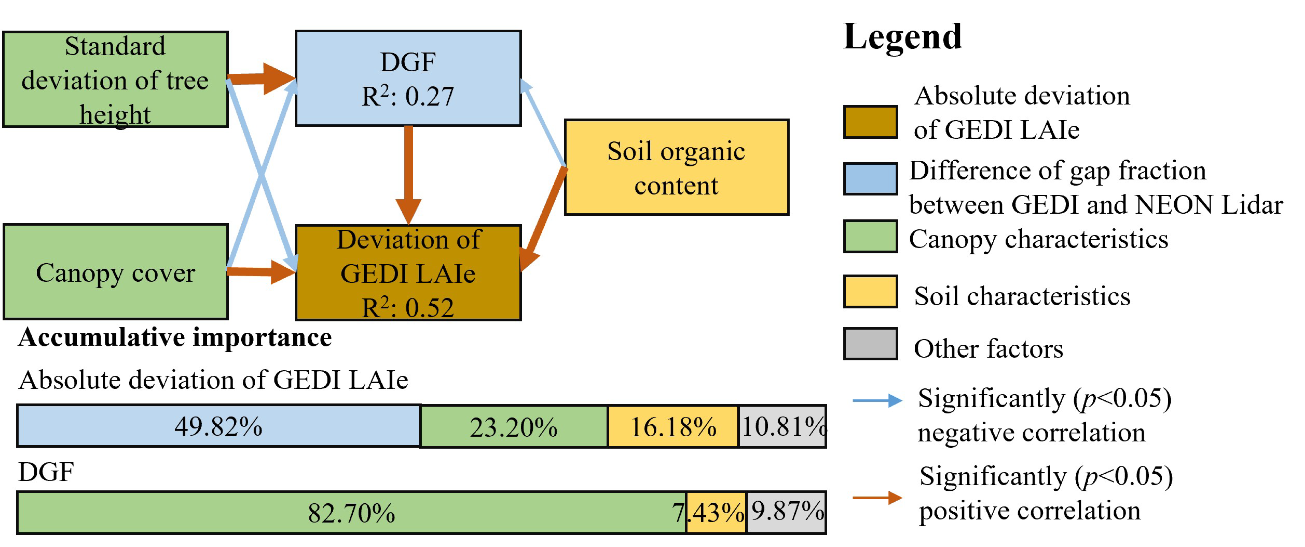
3.5. Effects of Factor Analysis for GEDI LAIe Estimation

The LMG was used to quantify the effect degree of each factor on the absolute deviation of GEDI LAIe (Figure 7, Supplementary Table S3). Results showed that the 19 factors moderately explained the absolute deviation of GEDI LAIe (R2: 0.52). Among factors, the DGF was the most important factor for the absolute deviation of GEDI LAIe, with its relative importance of 49%, followed by characteristics of canopy and soil with their relative importance of 23% and 16%, respectively. Consistent with the results of univariate analysis (see details in Supplementary file), characteristics of slope and sensor system parameters were relatively unimportant, with their relative importance near 10%.
The structural equation model was employed to clarify the direct and indirect effects of factors on the absolute deviation of GEDI LAIe (Figure 7, Supplementary Table S4). The parameters of the structural equation model were estimated using the maximum likelihood method. The χ 2 , χ 2 /df, GFI, AGFI, and RMSEA values were 7.11, 1.78, 0.98, 0.94, and 0.07, respectively. These accuracy metrics suggest that the formulated structural equation in this study met the model accuracy requirements. The SEM showed that only 4 out of 19 factors, including DGF, canopy cover, standard deviation of tree height, and soil organic content, had a significant and direct correlation with the absolute deviation of GEDI LAIe (p < 0.05).
The DGF acted as a pivot for the indirect impacts of canopy cover, standard deviation of tree height, and soil organic content on the absolute deviation of GEDI LAIe. That is, these factors indirectly affected the absolute deviation of GEDI LAIe by first affecting the DGF. All factors explained a total of 27% of the variation in DGF, among which canopy characteristics (relative importance of 82.70%) were the most important for DGF followed by soil characteristics. Specifically, the DGF decreased with the increase in canopy cover and soil organic content but increased with the increase in standard deviation of tree height.

3.6. Analysis of Effects of Clumping on Leaf Area Index of GEDI

The effectiveness of using the clumping indices of Ω footprint , Ω cover , and Ω crown for clumping correction in Fenghuang Mountains was analyzed in this study (Figure 8). Figure 8 shows different improvements when using different clumping indices. Specifically, without correction of clumping (when comparing GEDI LAIe to DHP LAIt), the values of bias, MAE, RMSE, %Bias, and %RMSE were −1.05 m2/m2, 1.05 m2/m2, 1.12 m2/m2, −0.56, and 0.6, respectively. After correcting the clumping between crowns using Ω cover , the values of absolute bias, MAE, and RMSE decreased by 0.05, 0.05, and 0.05 m2/m2, respectively. This fair improvement illustrates that within-crown clumping was dominant compared to between-crown clumping, in which the relative error of 93% was explained by within-crown clumping (Figure 8B). The above results illustrated that clumping correction was critical for GEDI LAI estimation, especially correction of within-crown clumping in temperate coniferous forests.

4. Discussion

4.1. Accuracy Analysis of GEDI LAIe Estimates

Reference data that are positionally accurate, spatially definite, and time-consistent over a large scale is the most challenging for the verification of GEDI LAIe [20,40]. The accuracy of the field-measured LAIe is high, but its high cost and intensive labor hinder its application over large areas [8,59]. Taking optical-based LAI products as a reference can cover a large area, but the assessment result suffered from uncertainties from the registration error, the large discrepancy of spatial scale, and errors of reference data [12]. Thus, using the field-measured LAIe or optical-based LAI products across a large area for assessing GEDI LAIe may be impractical [40,41].
Apart from 13 plots of field-measured LAIe derived from DHP images, NEON Lidar LAIe is regarded as the reference for evaluating GEDI LAIe [40,41] because (1) NEON Lidar LAIe is highly consistent with field-measured LAIe (Figure 2); (2) NEON Lidar covers various geographic units, with 47 typical terrestrial ecosystems across 20 climate zones in the United States; and (3) NEON Lidar has an accurate position which allows geolocation correction for GEDI waveforms by matching a GEDI waveform to a simulated waveform derived from NEON Lidar. Thus, using NEON Lidar LAIe as a reference to assess GEDI LAIe is technically persuasive and representative.
The high correlations of GEDI LAIe with NEON Lidar LAIe (r > 0.5, p < 0.05) (Figure 3, Figure 4, Figure 5 and Figure 6) and DHP LAIe collected in Fenghuang Mountains (0.71, Figure 3) were highly consistent with the widely recognized conclusion that large waveforms can measure LAIe effectively [7,11,68,69,70]. GEDI LAIe performance displayed a large discrepancy among different NEON sites (Figure 4) and forest types (Figure 5). The high values of RMSE in the eastern and western coastal NEON sites and broadleaf forests indicated that GEDI still faces challenges in dense forests with high LAI [23,69]. The moderate relative error of GEDI LAIe compared to NEON Lidar LAIe and DHP LAIe (%RMSE < 0.5) was in line with or even more appropriate for representing GEDI LAIe performance compared to the root mean squared percentage error of 3.83 reported in [19].

4.2. Analysis of Factors Affecting GEDI LAIe Estimation

This study clarified the mechanism and effect degree of factors on the error of GEDI LAIe based on a structural equation model and LMG (Figure 7). To the best of our knowledge, this paper is the first study to analyze the impact of multiple factors and their interactions on real GEDI LAIe estimation rather than pre-launched simulation analysis based on radiation transfer models and post-launched univariate analysis [19,20,33]. The analysis of factors affecting GEDI LAIe illustrated that the DGF is the dominant factor influencing GEDI LAIe estimation with a relative importance of nearly 50%, followed by canopy characteristics with a relative importance of 23%, and soil characteristics with a relative importance of 16%. In addition to a direct impact, canopy characteristics and soil characteristics have indirect influences on the absolute deviation of GEDI LAIe via DGF. Given that the ratio of vegetation and soil reflectance ( ρ v / ρ g ) is an essential term in gap fraction estimation using GORT [22], the canopy and soil characteristics indirectly impact GEDI LAIe through a direct effect on the gap fraction. The above results may shed a light on GEDI LAIe improvements by reducing DGF and uncertainty from the term of ρ v / ρ g . For example, Ni-Meister et al. (2010) proposed a method for the calculation of ρ v / ρ g using two adjacent footprints [71], which can be a potential solution for ρ v / ρ g estimation instead of a usage value of 1.5 in current GEDI LAIe product.
As the most important factor influencing GEDI LAIe estimation, about 27% of DGF variance can be explained by factors of sensor system parameters and characteristics of the canopy, soil, and topographic slope (Figure 7). The great unexplained DGF variance (73%) is probably initiated by systematic or stochastic uncertainties that are not a concern in this study [72]. It is an inherent bias in gap fraction estimation using different Lidar systems which use different concepts of ground returns [41]. NEON Lidar uses the ratio of returns from below 2 m to total returns for gap fraction estimation, which differs from the form of the ground-to-total energy ratio in GORT. Lacking knowledge of true ground returns for both NEON Lidar and GEDI is a potential risk for gap fraction estimation [41]. Luo et al. (2013) demonstrated that taking ground elevation as a threshold to separate ground energy from canopy energy can be site-suitable and lead to better LAI estimation [68]. With a large footprint being commensurate with canopy size, the full waveform can record more details of canopy elements than discrete point cloud Lidar, whose ability for LAIe estimation depends on point density [73]. Having the ability to detect small gaps, full waveform Lidar has more power penetration than discrete cloud point Lidar [72]. These above-mentioned uncertainties reasonably explained the DGF between GEDI and NEON Lidar that was unexplained by factors employed in this study.
Canopy characteristics, especially canopy cover and standard deviation of tree height, are important for both GEDI LAIe estimation and the DGF, with a relative importance of 23% and 82% (Figure 7), respectively. For the impact mechanism of canopy cover, the increase in canopy cover leads to a homogeneous forest resulting in a decrease in the DGF which narrows the absolute deviation of GEDI LAIe. The impact mechanism of the standard deviation of tree height on the DGF and GEDI LAIe estimation can owe to the vertical heterogeneity of the canopy. The increase in vertical heterogeneity of the canopy within the footprint increases the risk of under-sampling the canopy by discrete cloud Lidar compared to GEDI, which increases the DGF [70,73]. Moreover, the increasing vertical heterogeneity complicates the reflectance of the canopy, which can cause non-negligible multiple scattering in full-waveform Lidar [36,37]. The effect of multiple scattering for the DGF includes two scenarios. Firstly, multiple scattering forms pseudo-ground waveform peaks under the ground in large-footprint waveforms [7]. Using the pseudo-ground waveform energy instead of true ground waveform energy will result in an underestimation of the gap fraction [11,12]. Secondly, the energy of multiple scattering is not enough to form a pseudo-ground waveform peak but can exaggerate ground waveform energy. In this case, using the expanded ground waveform energy will cause the overestimation of the gap fraction in large footprint waveforms. Given that GEDI LAIe has a systematic underestimation in this study, it is reasonable to assume that the influence of multiple scattering on GEDI LAIe estimation follows the second scenario in most temperate forests.
Soil characteristics were regarded as a function of ground reflectance that directly affected gap fraction estimation using GORT. The relative importance of soil characteristics to GEDI LAIe estimation and the DGF is 16% and 7%, respectively. These results are comparable with previous studies [7,11,12,19] which reported an influence of 10~25% from the uncertainty of the ratio of ground and canopy reflectance ( ρ v / ρ g ) on LAIe estimation. The low relative importance value suggestes a limited influence of soil reflectance on estimates of gap fraction and LAIe using GEDI waveform in temperate forest areas [22].
Although the effect of topographic slope characteristics and sensor system parameters on the absolute deviation of GEDI LAIe and DGF was not significant in this study, the effect of these factors should not be ignored. For example, in a steep area, there is a risk of mixed energy of canopy and ground and a potential risk of interaction among factors, resulting in a reduction in accuracy of gap fraction estimation [19,30]. Additionally, this study found that the GEDI power beam outperformed the GEDI coverage beam, suggesting the potential for using sensor system parameters as a filter for an improvement of GEDI LAIe estimation.
Note that we analyzed the impact factors mainly based on NEON Lidar LAIe instead of field-measured datasets due to their limited number. Factors affecting the comparison of LAIe between GEDI and field plots should still be stressed. Specifically, the discrepancy caused by the mismatching of space and time directly undermined the assessment of GEDI LAIe (Supplementary Table S5). For example, without removing the outliers of field plots, the r, bias, MAE, RMSE, and %RMSE increased by 0.49, 0.04 m2/m2, 0.47 m2/m2, 0.47 m2/m2, and 0.32. Wang et al. (2022) [30] and Roy et al. (2021) [74] described how the influence of geolocation uncertainty of GEDI might be exaggerated by the high heterogeneity of the forest and topography. The high heterogeneity of forests caused by roads and buildings surrounding the 40 × 40 m plot (plot ID of 8, and 17–18 in Supplementary Figure S3) explained the LAIe difference between GEDI and field plots in the Fenghuang Mountains well. A steep slope (outside the 40 × 40 m plot) caused a change in the geometric relationship between vegetation and ground resulting in abnormal waveform peaks [40]. As a result, the GEDI LAIe substantially differed from field-measured LAIe (plot ID of 6 in Supplementary Table S5 and Figure S3). Thus, geolocation correction or selecting high-quality observations according to various factors such as slope are recommended for the better application of the GEDI LAIe product [30]. Although factor analysis based on NEON Lidar LAIe suggested that the influence of the difference in time between GEDI and NEON Lidar was insignificant (Figure 7, Supplementary Figure S2), a different phenomenon was found in Fenghuang Mountains. Specifically, a greater than 1 m2/m2 difference of LAIe between GEDI and field plots was found in deciduous forests, where GEDI and field plot data were collected in mid-April 2021 and early September 2022, respectively. Selecting a small-time interval between GEDI and its reference for accuracy assessment should be emphasized. Using a time-consistent NEON Lidar, the accuracy assessment result of GEDI LAIe in this study is more reliable than previous studies using relatively outdated reference data [19,20].

4.3. Limitations and Prospects

This study focused on the accuracy assessment of GEDI LAIe in mid-latitude temperate forests. Thus, our results cannot directly provide evidence for the performance of GEDI LAIe in tropical forests and boreal forests. Analysis of other factors related to LAI estimation should be conducted in future work. For example, the impact of the leaf inclination distribution function (G), which is a critical factor in Beer’s law, is not analyzed in this study due to the lack of an available proxy to characterize it. According to Jiang et al., setting the G function to 0.5 (i.e., spherical distribution) can cause a 53% error in GEDI LAIe estimation [35]. It is worth noting that GEDI LAIe is not the true leaf area within a footprint due to the clumping effect [6,33,66,67]. Taking field-measured LAIt as a reference, this study demonstrated a 0.81 relative error of GEDI LAIt estimation if the clumping effect is not corrected (Figure 8). This relative error is consistent with the 0.30~0.93 relative error reported in the previous study [8,33]. Moreover, our results showed that within-canopy clumping (relative errors of 0.79) is the dominant form of canopy clumping in coniferous forests, which is in line with [6,33,66]. Thus, future work is encouraged to correct the clumping effect for GEDI LAIt estimation.

5. Conclusions

GEDI has provided a near-global LAIe product that has the potential to revolutionize the limitations of optical-based LAIe estimation. A comprehensive accuracy assessment of GEDI LAIe products is a prerequisite for its appropriate application. This study makes a direct and indirect assessment of GEDI LAIe based on field survey datasets in Fenghuang Mountains and NEON Lidar LAIe over 22 NEON sites covering 12 forest types across the CONUS. Results showed a systematical underestimation of GEDI LAIe in temperate forests with a moderate error (%RMSE: 0.33~0.52). The performance of GEDI LAIe varied between forest types, with higher error in dense broadleaf forest compared to sparse coniferous forest. Analysis of the influence of factors revealed that the absolute deviation of GEDI LAIe was mostly impacted by the accuracy of the gap fraction (relative importance of 49%), followed by characteristics of canopy and soil with a relative importance of 23% and 16%, respectively. The vertical heterogeneity proxied by the standard deviation of the tree height and canopy cover is a non-negligible factor for estimates of GEDI LAIe and gap fraction. Findings in this study provide insight into the accuracy of GEDI LAIe for various forest types and geographic units and clarify the mechanism of multiple factors to GEDI LAIe, which are valuable for the application and improvement of GEDI LAIe.

Supplementary Materials

The following supporting information can be downloaded at: https://www.mdpi.com/article/10.3390/rs15061535/s1, Figure S1: Locations for taking DHP imageries within a plot; Figure S2. The relationship between the absolute deviation of GEDI LAIe (|Bias|) and factors; Figure S3. Accuracy comparison of GEDI LAIe between before and after filtering outliers when compared to filed-measured LAIe based on Digital Hemispherical Photography imageries. Table S1: The NEON AOP discrete LiDAR sites and their features; Table S2: Field-measured LAIe and LAIt corresponding to the 22 footprints of GEDI in the Fenghuang Mountains; Table S3. The relative importance of each factor for the absolute deviation of GEDI LAIe (referred to as LAIe deviation) and the difference between gap fraction derived from GEDI and NEON Lidar (referred to as DGF); Table S4. Path parameters in a structural equation model for GEDI LAIe deviation analysis; Table S5. Examples of forest landscape for GEDI footprint to conduct field survey and the corresponding GEDI waveform.

Author Contributions

Conceptualization, C.W. and D.J.; Funding acquisition, C.W. and D.J.; Methodology, C.W., D.J. and L.T.; Resources, C.W., D.J. and I.N.; Software, C.W. and D.J.; Supervision, D.J. and S.L.; Validation, C.W. and D.J.; Writing—original draft, C.W.; Writing—review and editing, C.W., D.J., I.N., S.L. and L.T. All authors have read and agreed to the published version of the manuscript.

Funding

This work is funded by the ‘Outstanding Innovation Scholarship for Doctoral Candidate of CUMT’ (Grant No. 2019YCBS054). The participation of Duo Jia was supported by China Postdoctoral Science Foundation (2022M723378). The participation of Izaya Numata was supported by NASA LCLUC (80NSSC20K0365).

Data Availability Statement

The raw discrete point cloud LiDAR (NEON LiDAR) and GEDI data were generated at the National Ecological Observation Network (NEON) and the Land Processes Distributed Active Archive Center (LP DAAC), respectively. Derived data supporting the findings of this study are available from the corresponding author on request.

Acknowledgments

Authors in this study particularly appreciate Andrew J. Elmore, Mark A. Cochrane, and Yuanyuan Li for their support in GEDI and field data collection.

Conflicts of Interest

The authors declare no conflict of interest.

References

  1. Chen, J.M.; Black, T.A. Defining leaf area index for non-flat leaves. Plant. Cell Environ. 1992, 15, 421–429. [Google Scholar] [CrossRef]
  2. Chen, J.M.; Ju, W.; Ciais, P.; Viovy, N.; Liu, R.; Liu, Y.; Lu, X. Vegetation structural change since 1981 significantly enhanced the terrestrial carbon sink. Nat. Commun. 2019, 10, 4259. [Google Scholar] [CrossRef] [PubMed] [Green Version]
  3. Fang, J.; Shugart, H.H.; Liu, F.; Yan, X.; Song, Y.; Lv, F. FORCCHN V2.0: An individual-based model for predicting multiscale forest carbon dynamics. Geosci. Model Dev. 2022, 15, 6863–6872. [Google Scholar] [CrossRef]
  4. Parker, G.G.; Lefsky, M.A.; Harding, D.J. Light transmittance in forest canopies determined using airborne laser altimetry and in-canopy quantum measurements. Remote Sens. Environ. 2001, 76, 298–309. [Google Scholar] [CrossRef]
  5. Hyde, P.; Dubayah, R.; Peterson, B.; Blair, J.B.; Hofton, M.; Hunsaker, C.; Knox, R.; Walker, W. Mapping forest structure for wildlife habitat analysis using waveform lidar: Validation of montane ecosystems. Remote Sens. Environ. 2005, 96, 427–437. [Google Scholar] [CrossRef]
  6. Hu, R.; Luo, J.; Yan, G.; Zou, J.; Mu, X. Indirect measurement of forest leaf area index using path length distribution model and multispectral canopy imager. IEEE J. Sel. Top. Appl. Earth Obs. Remote Sens. 2016, 9, 2532–2539. [Google Scholar] [CrossRef]
  7. Tang, H.; Brolly, M.; Zhao, F.; Strahler, A.H.; Schaaf, C.L.; Ganguly, S.; Zhang, G.; Dubayah, R. Deriving and validating Leaf Area Index (LAI) at multiple spatial scales through lidar remote sensing: A case study in Sierra National Forest, CA. Remote Sens. Environ. 2014, 143, 131–141. [Google Scholar] [CrossRef]
  8. Yan, G.; Hu, R.; Luo, J.; Weiss, M.; Jiang, H.; Mu, X.; Xie, D.; Zhang, W. Review of indirect optical measurements of leaf area index: Recent advances, challenges, and perspectives. Agric. For. Meteorol. 2019, 265, 390–411. [Google Scholar] [CrossRef]
  9. Wei, S.; Yin, T.; Dissegna, M.A.; Whittle, A.J.; Ow, G.L.F.; Yusof, M.L.M.; Lauret, N.; Gastellu-Etchegorry, J.P. An assessment study of three indirect methods for estimating leaf area density and leaf area index of individual trees. Agric. For. Meteorol. 2020, 292–293, 108101. [Google Scholar] [CrossRef]
  10. Fang, H.; Baret, F.; Plummer, S.; Schaepman-Strub, G. An Overview of Global Leaf Area Index (LAI): Methods, Products, Validation, and Applications. Rev. Geophys. 2019, 57, 739–799. [Google Scholar] [CrossRef]
  11. Tang, H.; Dubayah, R.; Swatantran, A.; Hofton, M.; Sheldon, S.; Clark, D.B.; Blair, B. Retrieval of vertical LAI profiles over tropical rain forests using waveform lidar at la selva, costa rica. Remote Sens. Environ. 2012, 124, 242–250. [Google Scholar] [CrossRef]
  12. Tang, H.; Dubayah, R.; Brolly, M.; Ganguly, S.; Zhang, G. Large-scale retrieval of leaf area index and vertical foliage profile from the spaceborne waveform lidar (GLAS/ICESat). Remote Sens. Environ. 2014, 154, 8–18. [Google Scholar] [CrossRef]
  13. Cui, L.; Guo, J.; Jiao, Z.; Sun, M.; Dong, Y.; Zhang, X.; Yin, S.; Chang, Y.; DIng, A.; Xie, R. Retrieval of the Forest Leaf Area Index Based on the Laser Penetration Ratio from the GLAS Waveform Lidar Data. In Proceedings of the IGARSS 2019-2019 IEEE International Geoscience and Remote Sensing Symposium, Yokohama, Japan, 28 July–2 August 2019; pp. 8972–8975. [Google Scholar] [CrossRef]
  14. Zhang, J.; Tian, J.; Li, X.; Wang, L.; Chen, B.; Gong, H.; Ni, R.; Zhou, B.; Yang, C. Leaf area index retrieval with ICESat-2 photon counting LiDAR. Int. J. Appl. Earth Obs. Geoinf. 2021, 103, 102488. [Google Scholar] [CrossRef]
  15. Dubayah, R.; Blair, J.B.; Goetz, S.; Fatoyinbo, L.; Hansen, M.; Healey, S.; Hofton, M.; Hurtt, G.; Kellner, J.; Luthcke, S.; et al. The Global Ecosystem Dynamics Investigation: High-resolution laser ranging of the Earth’s forests and topography. Sci. Remote Sens. 2020, 1, 100002. [Google Scholar] [CrossRef]
  16. Cui, L.; Jiao, Z.; Zhao, K.; Sun, M.; Dong, Y.; Yin, S. Index Using Transmitted Energy Information Derived from ICESat GLAS Data. Remote Sens. 2020, 12, 2457. [Google Scholar] [CrossRef]
  17. Yang, W.; Ni-Meister, W.; Lee, S. Assessment of the impacts of surface topography, off-nadir pointing and vegetation structure on vegetation lidar waveforms using an extended geometric optical and radiative transfer model. Remote Sens. Environ. 2011, 115, 2810–2822. [Google Scholar] [CrossRef]
  18. Yang, X.; Wang, C.; Xi, X.; Wang, Y.; Zhang, Y.; Zhou, G. Footprint Size Design of Large-Footprint Full-Waveform LiDAR for Forest and Topography Applications: A Theoretical Study. IEEE Trans. Geosci. Remote Sens. 2021, 59, 9745–9757. [Google Scholar] [CrossRef]
  19. Ilangakoon, N.; Glenn, N.F.; Schneider, F.D.; Dashti, H.; Hancock, S.; Spaete, L.; Goulden, T. Airborne and Spaceborne Lidar Reveal Trends and Patterns of Functional Diversity in a Semi-Arid Ecosystem. Front. Remote Sens. 2021, 2, 743320. [Google Scholar] [CrossRef]
  20. Dhargay, S.; Lyell, C.S.; Brown, T.P.; Inbar, A.; Sheridan, G.J.; Lane, P.N.J. Performance of GEDI Space-Borne LiDAR for Quantifying Structural Variation in the Temperate Forests of South-Eastern Australia. Remote Sens. 2022, 14, 3615. [Google Scholar] [CrossRef]
  21. Tang, H.; Armston, J. Algorithm Theoretical Basis Document (ATBD) for GEDI L2B Footprint Canopy Cover and Vertical Profile Metrics; Goddard Space Flight Center: Greenbelt, MD, USA, 2019. [Google Scholar]
  22. Ni-Meister, W.; Jupp, D.L.B.; Dubayah, R. Modeling lidar waveforms in heterogeneous and discrete canopies. IEEE Trans. Geosci. Remote Sens. 2001, 39, 1943–1958. [Google Scholar] [CrossRef] [Green Version]
  23. Rishmawi, K.; Huang, C.; Schleeweis, K.; Zhan, X. Integration of VIIRS Observations with GEDI-Lidar Measurements to Monitor Forest Structure Dynamics from 2013 to 2020 across the Conterminous United States. Remote Sens. 2022, 14, 2320. [Google Scholar] [CrossRef]
  24. Boucher, P.B.; Hancock, S.; Orwig, D.A.; Duncanson, L.; Armston, J.; Tang, H.; Krause, K.; Cook, B.; Paynter, I.; Li, Z.; et al. Detecting change in forest structure with simulated GEDI lidarwaveforms: A case study of the hemlock woolly adelgid (HWA; adelges tsugae) infestation. Remote Sens. 2020, 12, 1304. [Google Scholar] [CrossRef] [Green Version]
  25. Sanchez-Lopez, N.; Boschetti, L.; Hudak, A.T.; Hancock, S.; Duncanson, L.I. Estimating time since the last stand-replacing disturbance (TSD) from spaceborne simulated GEDI data: A feasibility study. Remote Sens. 2020, 12, 3506. [Google Scholar] [CrossRef]
  26. Wang, C.; Elmore, A.J.; Numata, I.; Cochrane, M.A.; Lei, S.; Hakkenberg, C.R.; Li, Y.; Zhao, Y.; Tian, Y. A Framework for Improving Wall-to-Wall Canopy Height Mapping by Integrating GEDI LiDAR. Remote Sens. 2022, 14, 3618. [Google Scholar] [CrossRef]
  27. Schimel, D.; Hargrove, W.; Hoffman, F.; MacMahon, J. NEON: A hierarchically designed national ecological network. Front. Ecol. Environ. 2007, 5, 59. [Google Scholar] [CrossRef]
  28. Ordway, E.M.; Elmore, A.J.; Kolstoe, S.; Quinn, J.E.; Swanwick, R.; Cattau, M.; Taillie, D.; Guinn, S.M.; Chadwick, K.D.; Atkins, J.W.; et al. Leveraging the NEON Airborne Observation Platform for socio-environmental systems research. Ecosphere 2021, 12, e03640. [Google Scholar] [CrossRef]
  29. Hakkenberg, C.R.; Goetz, S.J. Climate mediates the relationship between plant biodiversity and forest structure across the United States. Glob. Ecol. Biogeogr. 2021, 30, 2245–2258. [Google Scholar] [CrossRef]
  30. Wang, C.; Elmore, A.J.; Numata, I.; Cochrane, M.A.; Shaogang, L.; Huang, J.; Zhao, Y.; Li, Y. Factors affecting relative height and ground elevation estimations of GEDI among forest types across the conterminous USA. GIScience Remote Sens. 2022, 59, 975–999. [Google Scholar] [CrossRef]
  31. Liu, A.; Cheng, X.; Chen, Z.; Liu, A. Performance evaluation of GEDI and ICESat-2 laser altimeter data for terrain and canopy height retrievals. Remote Sens. Environ. 2021, 264, 112571. [Google Scholar] [CrossRef]
  32. Kang, Y.; Ozdogan, M.; Gao, F.; Anderson, M.C.; White, W.A.; Yang, Y.; Yang, Y.; Erickson, T.A. A data-driven approach to estimate leaf area index for Landsat images over the contiguous US. Remote Sens. Environ. 2021, 258, 112383. [Google Scholar] [CrossRef]
  33. Jiang, H.; Cheng, S.; Yan, G.; Kuusk, A.; Hu, R.; Tong, Y.; Mu, X.; Xie, D.; Zhang, W.; Zhou, G.; et al. Clumping Effects in Leaf Area Index Retrieval from Large-Footprint Full-Waveform LiDAR. IEEE Trans. Geosci. Remote Sens. 2022, 60, 4406220. [Google Scholar] [CrossRef]
  34. Jiang, H.; Yan, G.; Tong, Y.; Cheng, S.; Yang, X.; Hu, R.; Li, L.; Mu, X.; Xie, D.; Zhang, W.; et al. Correcting Crown-Level Clumping Effect for Improving Leaf Area Index Retrieval from Large-Footprint LiDAR: A Study Based on the Simulated Waveform and GLAS Data. IEEE J. Sel. Top. Appl. Earth Obs. Remote Sens. 2021, 14, 12386–12402. [Google Scholar] [CrossRef]
  35. Yan, G.; Jiang, H.; Luo, J.; Mu, X.; Li, F.; Qi, J.; Hu, R.; Xie, D.; Zhou, G. Quantitative Evaluation of Leaf Inclination Angle Distribution on Leaf Area Index Retrieval of Coniferous Canopies. J. Remote Sens. 2021, 2021, 2708904. [Google Scholar] [CrossRef]
  36. Calders, K.; Lewis, P.; Disney, M.; Verbesselt, J.; Herold, M. Investigating assumptions of crown archetypes for modelling LiDAR returns. Remote Sens. Environ. 2013, 134, 39–49. [Google Scholar] [CrossRef]
  37. Gastellu-Etchegorry, J.P.; Yin, T.; Lauret, N.; Grau, E.; Rubio, J.; Cook, B.D.; Morton, D.C.; Sun, G. Simulation of satellite, airborne and terrestrial LiDAR with DART (I): Waveform simulation with quasi-Monte Carlo ray tracing. Remote Sens. Environ. 2016, 184, 418–435. [Google Scholar] [CrossRef]
  38. Mitchell, P.J.; Benyon, R.G.; Lane, P.N.J. Responses of evapotranspiration at different topographic positions and catchment water balance following a pronounced drought in a mixed species eucalypt forest, Australia. J. Hydrol. 2012, 440–441, 62–74. [Google Scholar] [CrossRef]
  39. Chen, J.M.; Menges, C.H.; Leblanc, S.G. Global mapping of foliage clumping index using multi-angular satellite data. Remote Sens. Environ. 2005, 97, 447–457. [Google Scholar] [CrossRef]
  40. Mallet, C.; Bretar, F. Full-waveform topographic lidar: State-of-the-art. ISPRS J. Photogramm. Remote Sens. 2009, 64, 1–16. [Google Scholar] [CrossRef]
  41. Wang, Y.; Fang, H. Estimation of LAI with the LiDAR technology: A review. Remote Sens. 2020, 12, 3457. [Google Scholar] [CrossRef]
  42. Luthcke, S.B.; Rebold, T.; Thomas, T.; Pennington, T. Algorithm Theoretical Basis Document (ATBD) for GEDI Waveform Geolocation for L1 and L2 Products; Goddard Space Flight Center: Greenbelt, MD, USA, 2019. [Google Scholar]
  43. Potapov, P.; Li, X.; Hernandez-Serna, A.; Tyukavina, A.; Hansen, M.C.; Kommareddy, A.; Pickens, A.; Turubanova, S.; Tang, H.; Silva, C.E.; et al. Mapping global forest canopy height through integration of GEDI and Landsat data. Remote Sens. Environ. 2021, 253, 112165. [Google Scholar] [CrossRef]
  44. Hansen, C.M.; Healey, S.; Hofton, M.; Hurtt, G.; Fatoyinbo, L.; Kellner, J.; Luthcke, S.; Armston, J.; Burns, P.; Duncanson, L.; et al. Global Ecosystem Dynamics Investigation (GEDI) Level 1B User Guide For SDPS PGEVersion 3 (P003) of GEDI L1B Data Science Team. Sci. Remote Sens. 2020, 3, 1–13. [Google Scholar]
  45. Blair, J.B.; Hofton, M.A. Modeling laser altimeter return waveforms over complex vegetation using high-resolution elevation data. Geophys. Res. Lett. 1999, 26, 2509–2512. [Google Scholar] [CrossRef]
  46. Hancock, S.; Armston, J.; Hofton, M.; Sun, X.; Tang, H.; Duncanson, L.I.; Kellner, J.R.; Dubayah, R. The GEDI Simulator: A Large-Footprint Waveform Lidar Simulator for Calibration and Validation of Spaceborne Missions. Earth Space Sci. 2019, 6, 294–310. [Google Scholar] [CrossRef] [PubMed]
  47. NEON (National Ecological Observatory Network). Discrete Return LiDAR Point Cloud (DP1.30003.001), RELEASE-2022. Available online: https://data.neonscience.org (accessed on 25 December 2022). [CrossRef]
  48. NEON (National Ecological Observatory Network). Digital Hemispheric Photos of Plot Vegetation (DP1.10017.001), RELEASE-2023. Available online: https://data.neonscience.org (accessed on 31 January 2023). [CrossRef]
  49. NEON (National Ecological Observatory Network). Elevation—LiDAR (DP3.30024.001), RELEASE-2022. Available online: https://data.neonscience.org (accessed on 25 December 2022). [CrossRef]
  50. Weinstein, B.G.; Marconi, S.; Bohlman, S.; Zare, A.; White, E. Individual tree-crown detection in rgb imagery using semi-supervised deep learning neural networks. Remote Sens. 2019, 11, 1309. [Google Scholar] [CrossRef] [Green Version]
  51. Weinstein, B.G.; Marconi, S.; Bohlman, S.A.; Zare, A.; White, E.P. Cross-site learning in deep learning RGB tree crown detection. Ecol. Inform. 2020, 56, 101061. [Google Scholar] [CrossRef]
  52. Weinstein, B.G.; Marconi, S.; Aubry-Kientz, M.; Vincent, G.; Senyondo, H.; White, E.P. DeepForest: A Python package for RGB deep learning tree crown delineation. Methods Ecol. Evol. 2020, 11, 1743–1751. [Google Scholar] [CrossRef]
  53. Weiss, M.; Baret, F. CAN_EYE V6.4.91 User Manual; HAL Open Science: Lyon, France, 2017; pp. 1–20. [Google Scholar]
  54. Riaño, D.; Valladares, F.; Condés, S.; Chuvieco, E. Estimation of leaf area index and covered ground from airborne laser scanner (Lidar) in two contrasting forests. Agric. For. Meteorol. 2004, 124, 269–275. [Google Scholar] [CrossRef]
  55. Liu, J.; Li, L.; Akerblom, M.; Wang, T.; Skidmore, A.; Zhu, X.; Heurich, M. Comparative evaluation of algorithms for leaf area index estimation from digital hemispherical photography through virtual forests. Remote Sens. 2021, 13, 3325. [Google Scholar] [CrossRef]
  56. Weiss, M.; Baret, F.; Smith, G.J.; Jonckheere, I.; Coppin, P. Review of methods for in situ leaf area index (LAI) determination Part II. Estimation of LAI, errors and sampling. Agric. For. Meteorol. 2004, 121, 37–53. [Google Scholar] [CrossRef]
  57. Blackard, J.A.; Finco, M.V.; Helmer, E.H.; Holden, G.R.; Hoppus, M.L.; Jacobs, D.M.; Lister, A.J.; Moisen, G.G.; Nelson, M.D.; Riemann, R.; et al. Mapping U.S. forest biomass using nationwide forest inventory data and moderate resolution information. Remote Sens. Environ. 2008, 112, 1658–1677. [Google Scholar] [CrossRef]
  58. Hengl, T.; De Jesus, J.M.; Heuvelink, G.B.M.; Gonzalez, M.R.; Kilibarda, M.; Blagotić, A.; Shangguan, W.; Wright, M.N.; Geng, X.; Bauer-Marschallinger, B.; et al. SoilGrids250m: Global Gridded Soil Information Based on Machine Learning. PLoS ONE 2017, 12, e0169748. [Google Scholar] [CrossRef] [Green Version]
  59. Tian, L.; Qu, Y.; Qi, J. Estimation of forest lai using discrete airborne lidar: A review. Remote Sens. 2021, 13, 2408. [Google Scholar] [CrossRef]
  60. Armston, J.; Disney, M.; Lewis, P.; Scarth, P.; Phinn, S.; Lucas, R.; Bunting, P.; Goodwin, N. Direct retrieval of canopy gap probability using airborne waveform lidar. Remote Sens. Environ. 2013, 134, 24–38. [Google Scholar] [CrossRef]
  61. Wagner, W.; Ullrich, A.; Ducic, V.; Melzer, T.; Studnicka, N. Gaussian decomposition and calibration of a novel small-footprint full-waveform digitising airborne laser scanner. ISPRS J. Photogramm. Remote Sens. 2006, 60, 100–112. [Google Scholar] [CrossRef]
  62. Grömping, U. Relative importance for linear regression in R: The package relaimpo. J. Stat. Softw. 2006, 17, 1–27. [Google Scholar] [CrossRef] [Green Version]
  63. Gough, C.M.; Atkins, J.W.; Fahey, R.T.; Hardiman, B.S. High rates of primary production in structurally complex forests. Ecology 2019, 100, e02864. [Google Scholar] [CrossRef] [Green Version]
  64. Murphy, B.A.; May, J.A.; Butterworth, B.J.; Andresen, C.G.; Desai, A.R. Unraveling Forest Complexity: Resource Use Efficiency, Disturbance, and the Structure-Function Relationship. J. Geophys. Res. Biogeosci. 2022, 127, e2021JG006748. [Google Scholar] [CrossRef]
  65. Chen, J.M.; Cihlar, J. Quantifying the Effect of Canopy Architecture on Optical Measurements of Leaf Area Index Using Two Gap Size Analysis Methods. IEEE Trans. Geosci. Remote Sens. 1995, 33, 777–787. [Google Scholar] [CrossRef]
  66. Hu, R.; Yan, G.; Nerry, F.; Liu, Y.; Jiang, Y.; Wang, S.; Chen, Y.; Mu, X.; Zhang, W.; Xie, D. Using Airborne Laser Scanner and Path Length Distribution Model to Quantify Clumping Effect and Estimate Leaf Area Index. IEEE Trans. Geosci. Remote Sens. 2018, 56, 3196–3209. [Google Scholar] [CrossRef]
  67. Yang, X.; Wang, C.; Pan, F.; Nie, S.; Xi, X.; Luo, S. Retrieving leaf area index in discontinuous forest using ICESat/GLAS full-waveform data based on gap fraction model. ISPRS J. Photogramm. Remote Sens. 2019, 148, 54–62. [Google Scholar] [CrossRef]
  68. Luo, S.; Wang, C.; Li, G.; Xi, X. Retrieving leaf area index using ICESat/GLAS full-waveform data. Remote Sens. Lett. 2013, 4, 745–753. [Google Scholar] [CrossRef]
  69. Tang, H.; Ganguly, S.; Zhang, G.; Hofton, M.A.; Nelson, R.F.; Dubayah, R. Characterizing leaf area index (LAI) and vertical foliage profile (VFP) over the United States. Biogeosciences 2016, 13, 239–252. [Google Scholar] [CrossRef] [Green Version]
  70. Tian, J.; Wang, L.; Li, X.; Shi, C.; Gong, H. Differentiating Tree and Shrub LAI in a Mixed Forest with ICESat/GLAS Spaceborne LiDAR. IEEE J. Sel. Top. Appl. Earth Obs. Remote Sens. 2017, 10, 87–94. [Google Scholar] [CrossRef]
  71. Ni-Meister, W.; Lee, S.; Strahler, A.H.; Woodcock, C.E.; Schaaf, C.; Yao, T.; Ranson, K.J.; Sun, G.; Blair, J.B. Assessing general relationships between aboveground biomass and vegetation structure parameters for improved carbon estimate from lidar remote sensing. J. Geophys. Res. Biogeosci. 2010, 115, G00E11. [Google Scholar] [CrossRef] [Green Version]
  72. Mahoney, C.; Hopkinson, C.; Kljun, N.; van Gorsel, E. Estimating canopy gap fraction using ICESat GLAS within Australian forest ecosystems. Remote Sens. 2017, 9, 59. [Google Scholar] [CrossRef] [Green Version]
  73. Zhao, F.; Yang, X.; Strahler, A.H.; Schaaf, C.L.; Yao, T.; Wang, Z.; Román, M.O.; Woodcock, C.E.; Ni-Meister, W.; Jupp, D.L.B.; et al. A comparison of foliage profiles in the Sierra National Forest obtained with a full-waveform under-canopy EVI lidar system with the foliage profiles obtained with an airborne full-waveform LVIS lidar system. Remote Sens. Environ. 2013, 136, 330–341. [Google Scholar] [CrossRef] [Green Version]
  74. Roy, D.P.; Kashongwe, H.B.; Armston, J.; Pot, D. The impact of geolocation uncertainty on GEDI tropical forest canopy height estimation and change monitoring. Sci. Remote Sens. 2021, 4, 100024. [Google Scholar] [CrossRef]
Figure 1. The distribution of study areas (A) including 22 NEON sites across the CONUS (B) and field-measured plots located in the Fenghuang Mountains in China (C). The red points in (A) were NEON sites in the COUNS and location of the Fenghuang Mountains in China. The numbers in (B) were identifications for the eco-climate region in the U.S.A. The red rectangle in (C) was the boundary for the field survey around the Fenghuang Mountains, while the red points in (C) were plot locations. The white number showed the field plot ID. The true color images were downloaded from google maps.
Remotesensing 15 01535 g001
Figure 2. Comparison of NEON Lidar LAIe and NEON DHP LAIe. The bias greater than 0 indicates that NEON Lidar overestimated LAIe compared to DHP LAIe, and vice versa. The black and red solid lines are the 1:1 line and regression line, respectively.
Remotesensing 15 01535 g002
Figure 3. Comparison of LAIe between GEDI and DHP images. The black and red solid lines are the 1:1 line and regression line, respectively.
Remotesensing 15 01535 g003
Figure 4. Comparison of LAIe between GEDI and NEON Lidar among the 22 NEON sites. The top map shows the spatial distribution of accuracy metrics among the NEON sites. The black and red solid lines in scatter plot are the 1:1 line and regression line, respectively. The scatter plots and histogram show the LAIe difference between GEDI and NEON Lidar, respectively. Each scatter plot represented a NEON site with its name marked in the gray rectangle.
Remotesensing 15 01535 g004
Figure 5. Comparison of LAIe between GEDI and NEON Lidar among forest types. Each scatter plot indicated a forest type with its name marked by a gray rectangle. The black and red solid lines are the 1:1 line and regression line, respectively.
Remotesensing 15 01535 g005
Figure 6. Values of GEDI LAIe among forest types. The values from 1 to 12 on the X-axis represented forest types of Longleaf/Slash Pine, Loblolly/Shortleaf Pine, Ponderosa Pine, Lodgepole Pine, Douglas-fir, Fir/Spruce/Mountain Hemlock, California Mixed Conifer, Oak/Pine, Aspen/Birch, Oak/Hickory, Oak/Gum/Cypress, and Maple/Beech/Birch, respectively.
Remotesensing 15 01535 g006
Figure 7. Structural equation model for explaining the direct and indirect effect of factors on the absolute deviation of GEDI LAIe. Different colored boxes represented categories of factors (see Table 1). Light blue and brown arrows show a significant negative and positive correlation between factors, respectively. The R2 and relative importance were calculated by IMG. Other factors included the characteristics of topographic slope and sensor system parameters.
Remotesensing 15 01535 g007
Figure 8. The influence (A) and relative errors (B) of the clumping effect. The black and red solid lines in (A) are the 1:1 line and regression line, respectively. The relative error is caused by clumping in different scales, such as footprint (overall), between crowns (between), and within crowns (within).
Remotesensing 15 01535 g008
Table 1. Definition and data sources of factors potentially affecting the absolute deviation of GEDI LAIe used in factor importance analysis.
CategoriesFactorsData SourceCategoriesFactorsData Source
DGFDGFGEDI L2B and NEON LidarTopographic slopeSlope (°)NEON DTM
CanopyForest typesForest type inventoryStandard deviation of slope
Canopy coverField of landsat_treecover in GEDI L2BSensor system parametersSensitivity (0.9–1.0)GEDI L2B
Mean height of trees (m)NEON’s individual tree productObservation time (day and night)
Standard deviation of tree heightBeam type (power beam and coverage beam)
Number of treesModes in waveform (1–20)
Standard deviation of crown areaPoint density of NEON Lidar (point/m2)NEON Lidar
SoilSoil nitrogen content (g/kg)Soilgrids dataScan angle (°)
Soil organic content (kg/kg)Difference of time between GEDI and NEON Lidar (Day of year)GEDI and NEON
Soil pH
Disclaimer/Publisher’s Note: The statements, opinions and data contained in all publications are solely those of the individual author(s) and contributor(s) and not of MDPI and/or the editor(s). MDPI and/or the editor(s) disclaim responsibility for any injury to people or property resulting from any ideas, methods, instructions or products referred to in the content.

