
Region-Specific and Weather-Dependent Characteristics of the Relation between GNSS-Weighted Mean Temperature and Surface Temperature over China

 ,
,  , ,
, ,
Abstract
:1. Introduction
2. Methods and Data
2.1. Role of in GNSS Water Vapor Retrieving
2.2. Determination of Linear Models
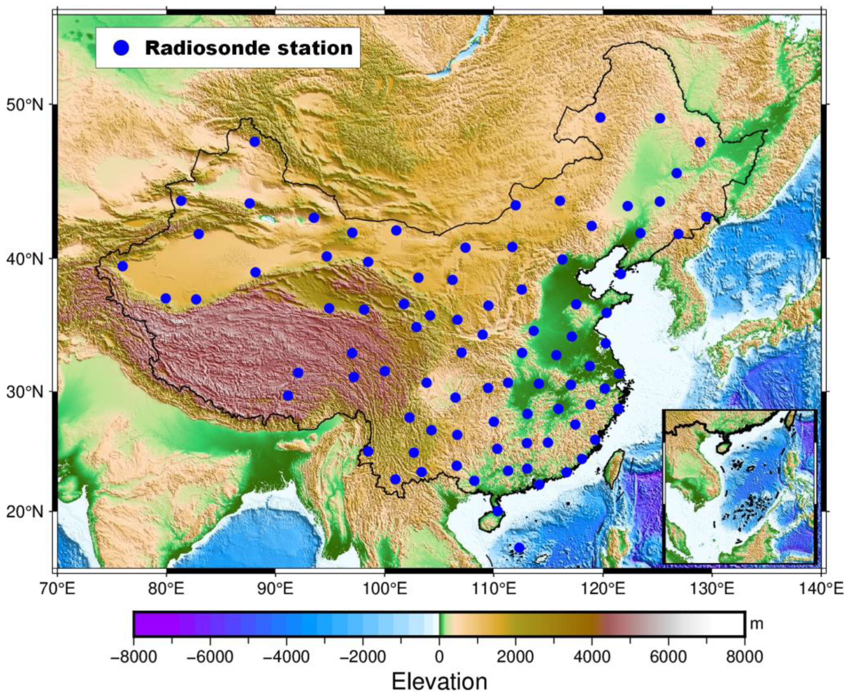
2.3. Radiosonde Data
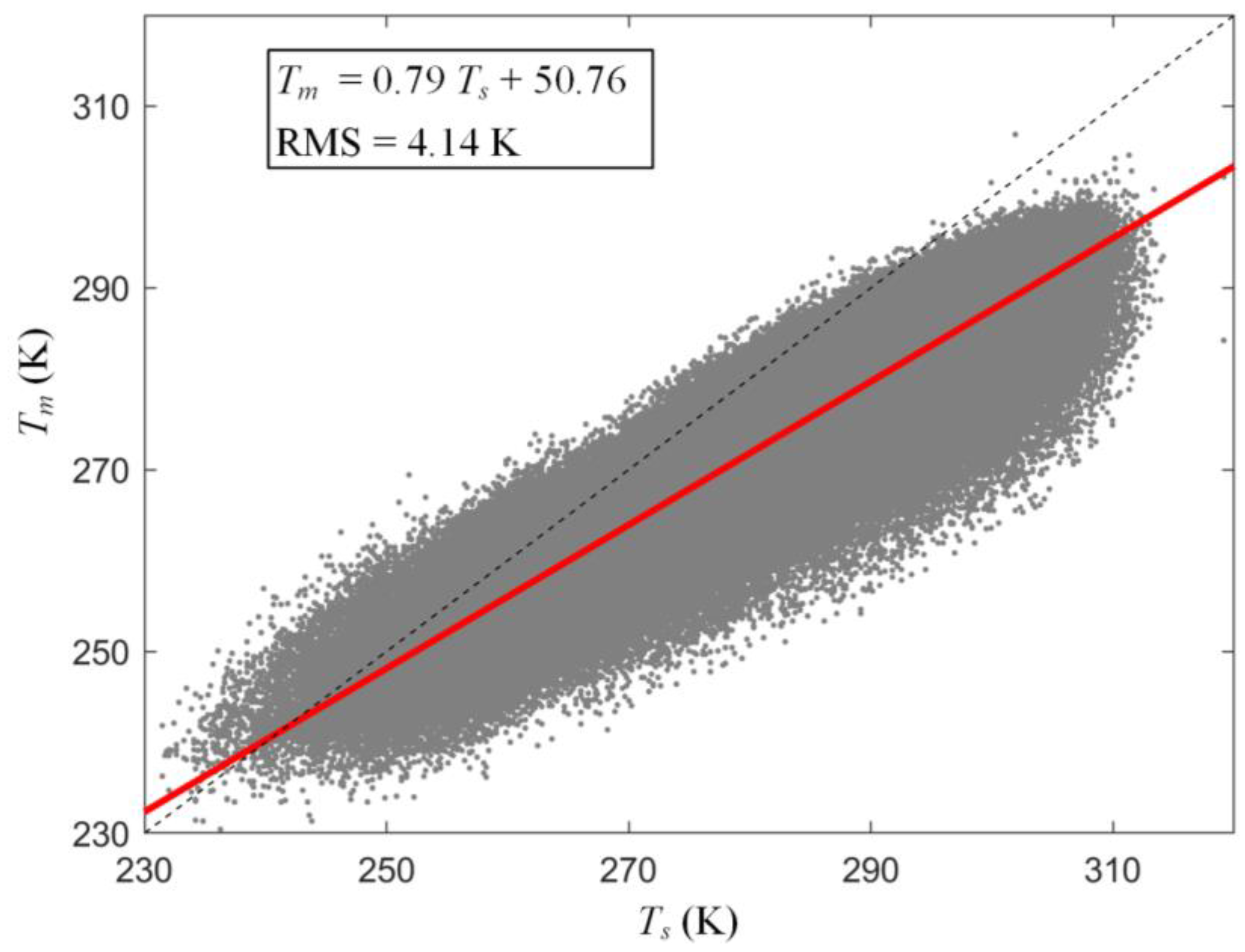
3. Unified Model
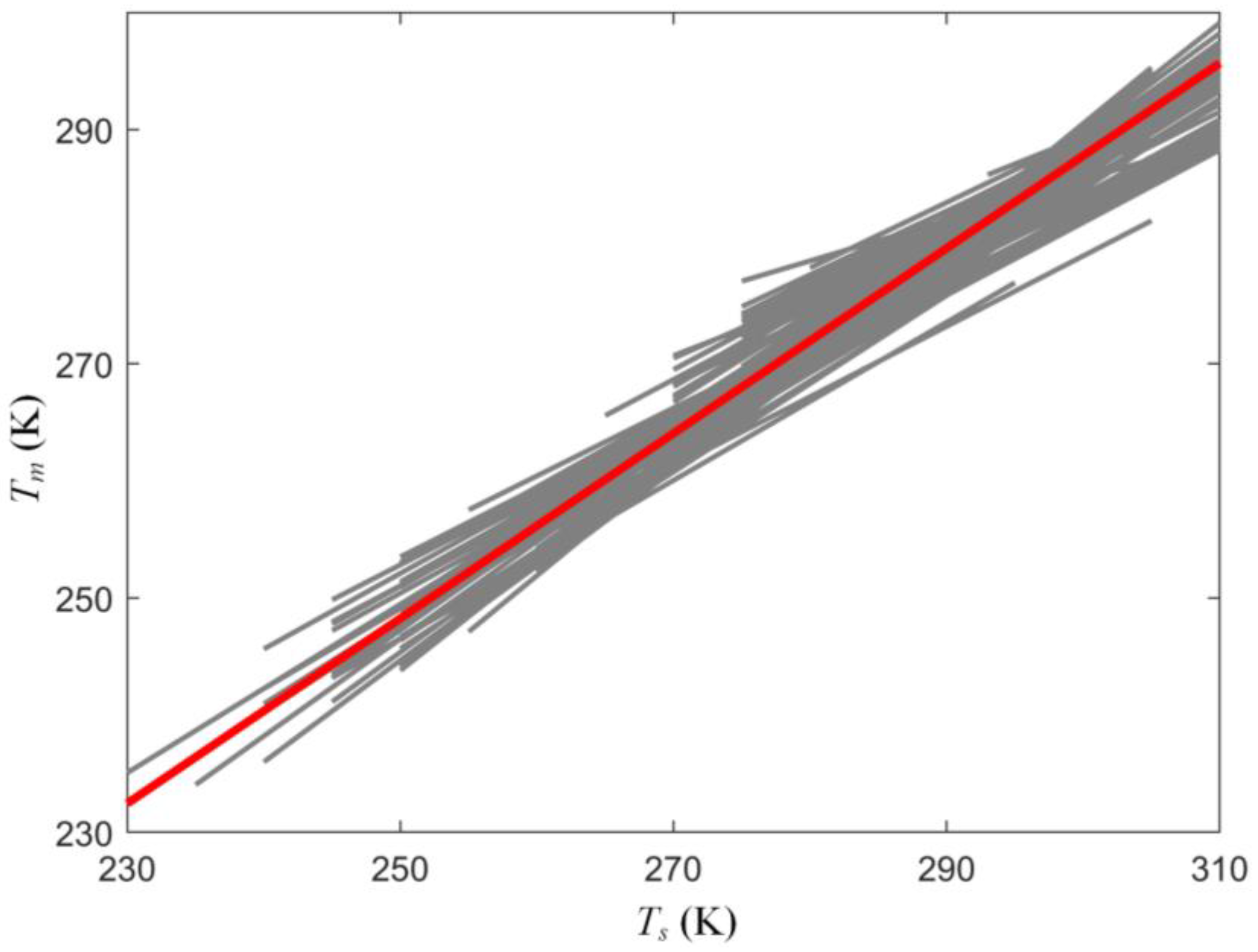
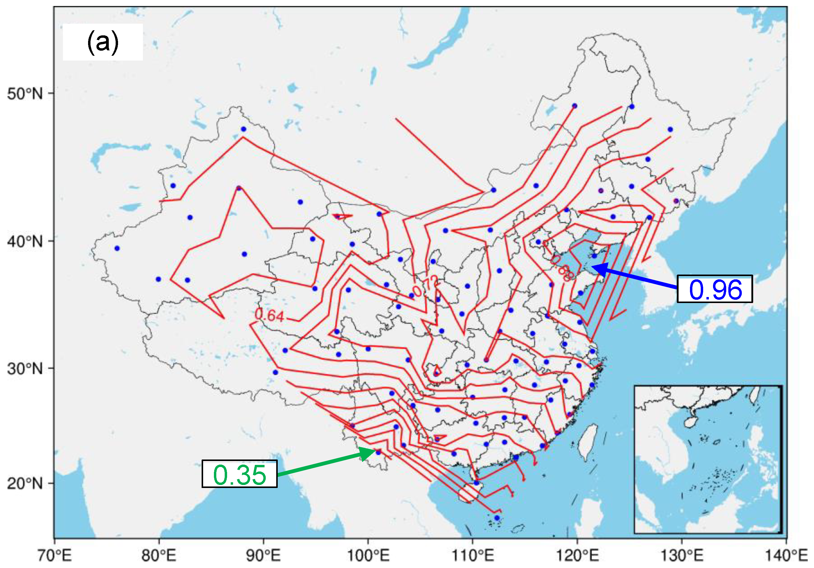
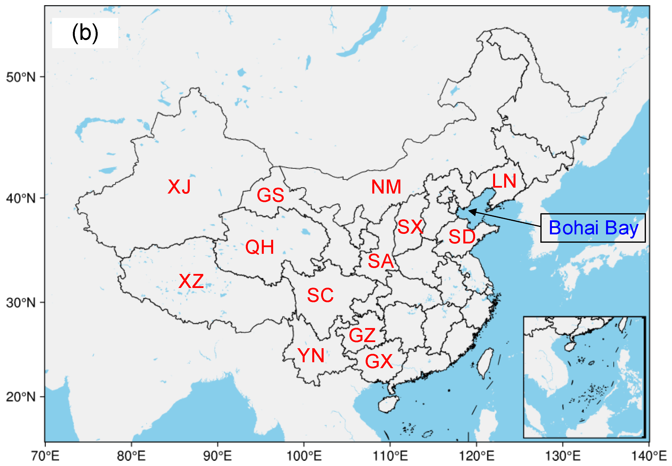
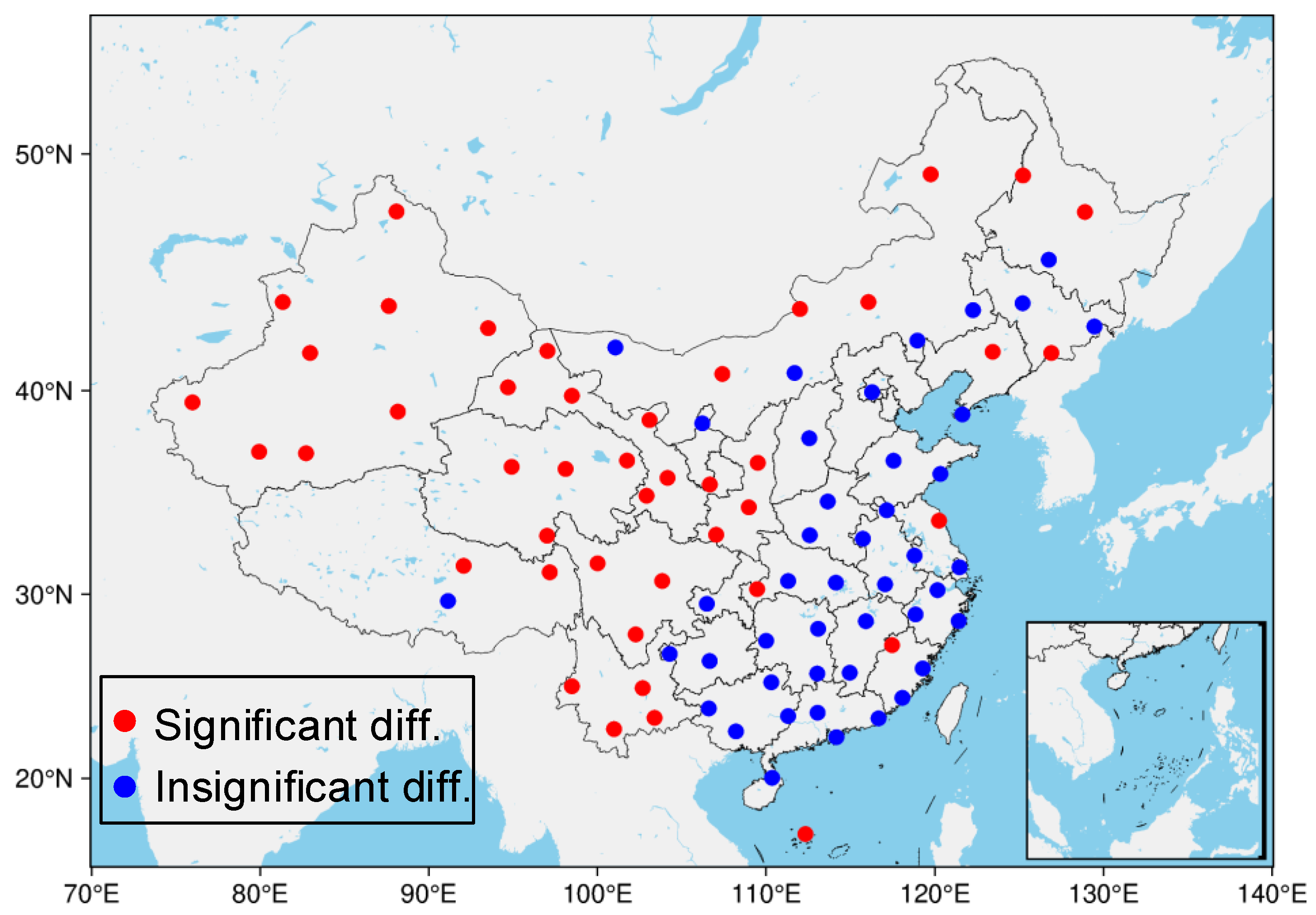
4. Region-Specific Characteristics of Linear Relations
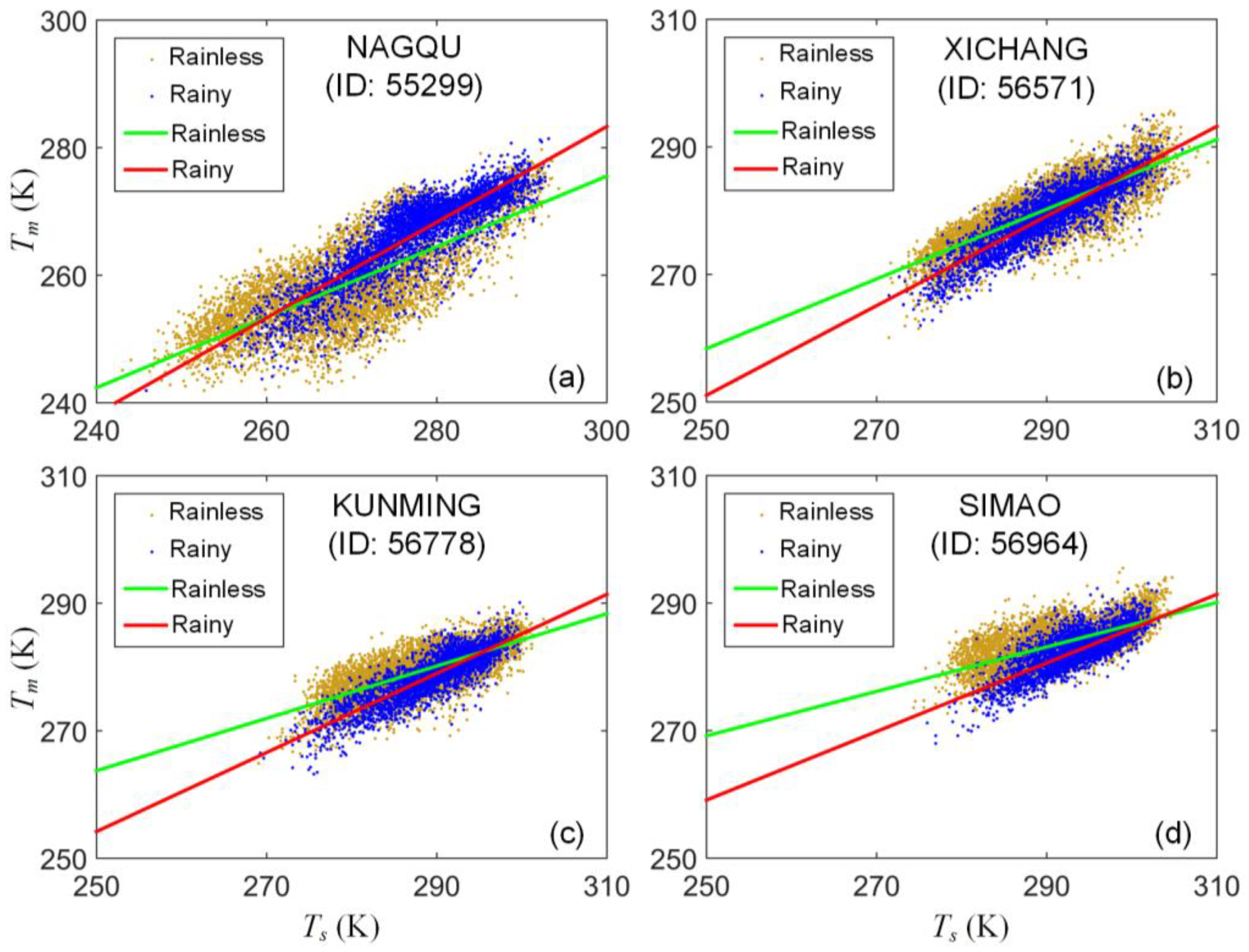
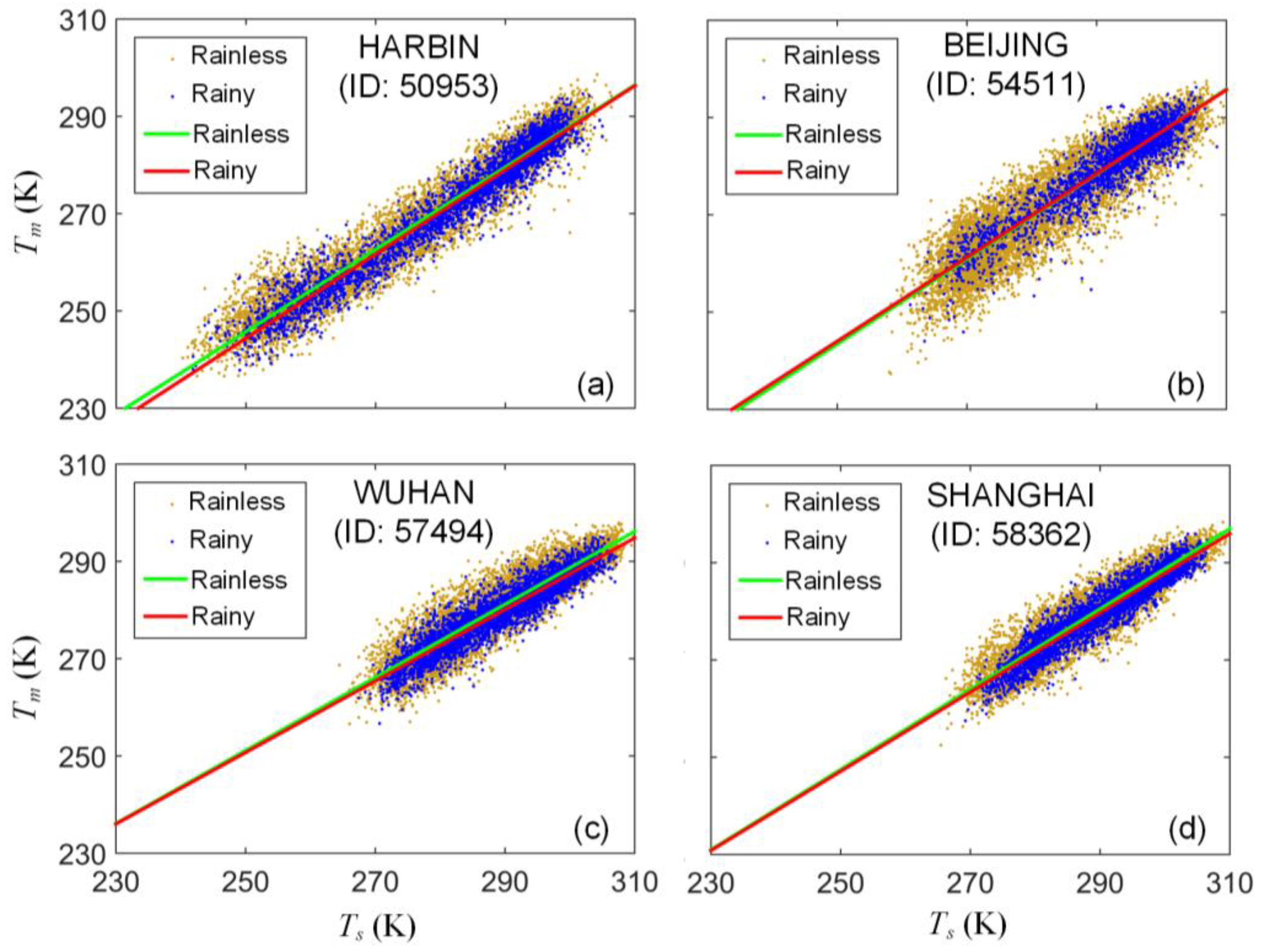
5. Weather-Dependent Characteristics of Linear Relations
5.1. Weather-Dependent Linear Models
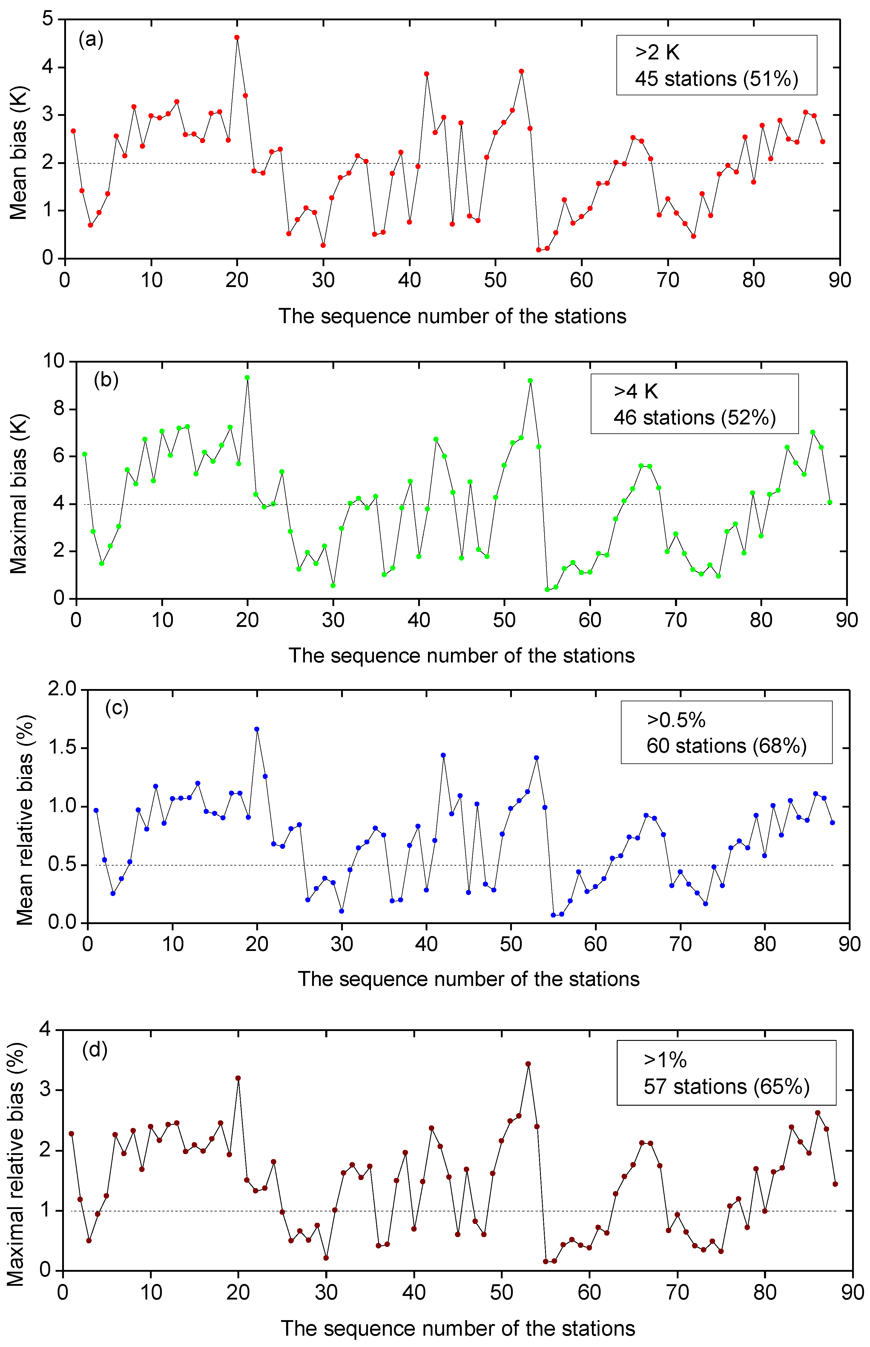
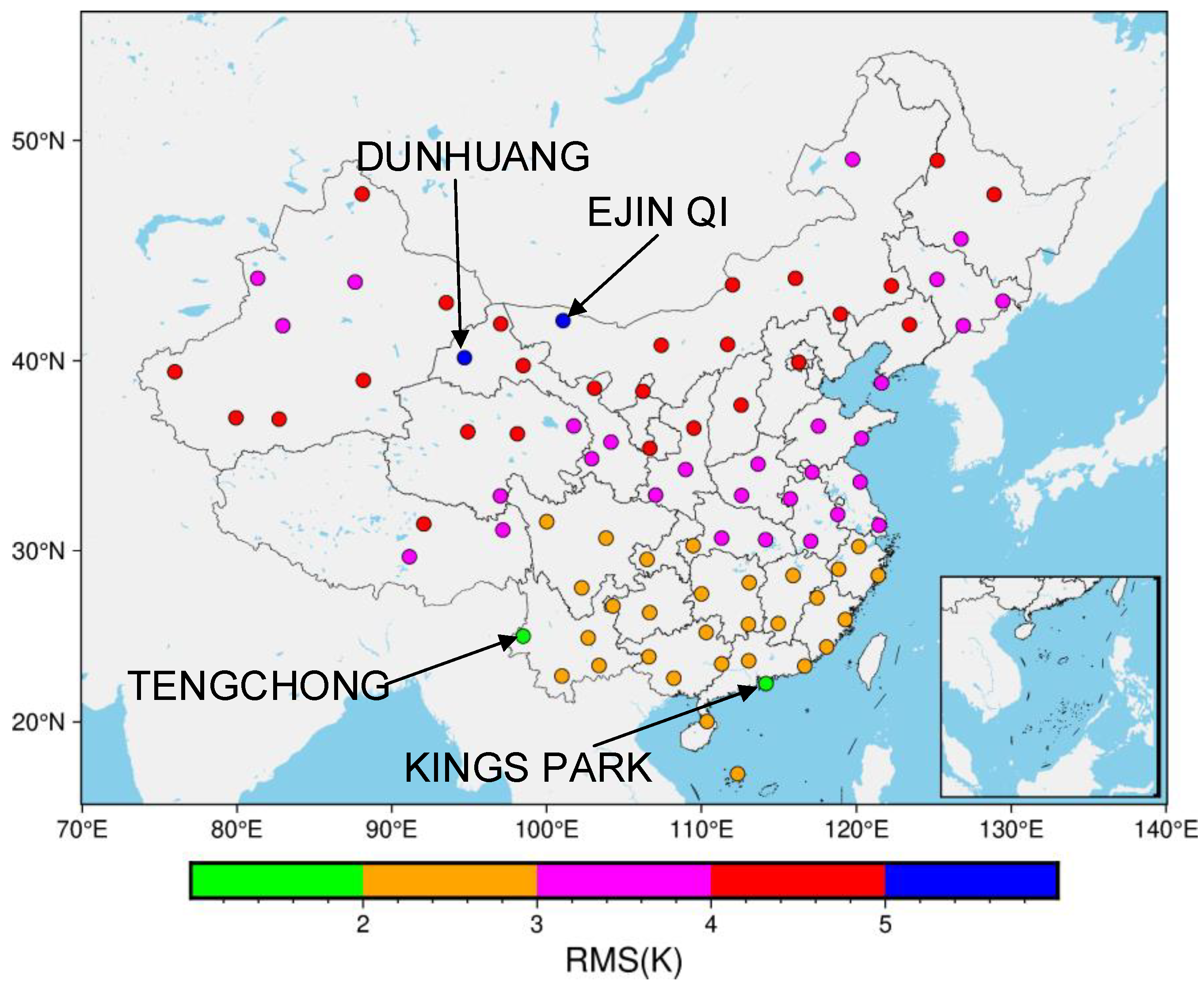
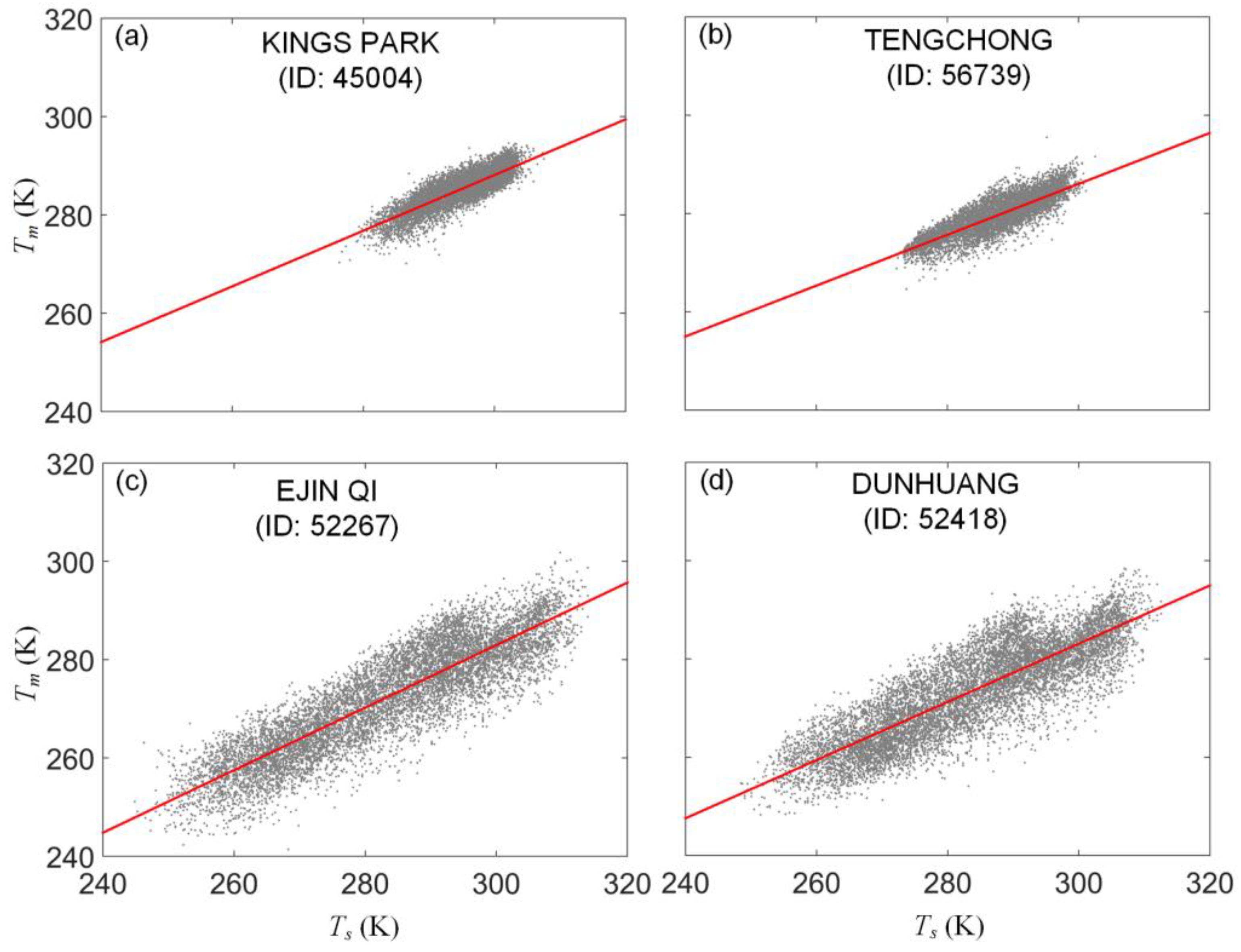
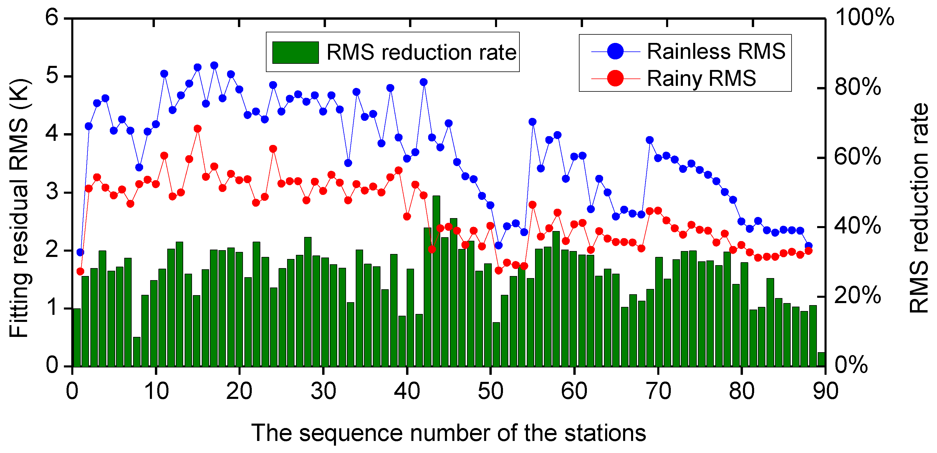
5.2. Comparison of Regression Precision of Weather-Dependent Models
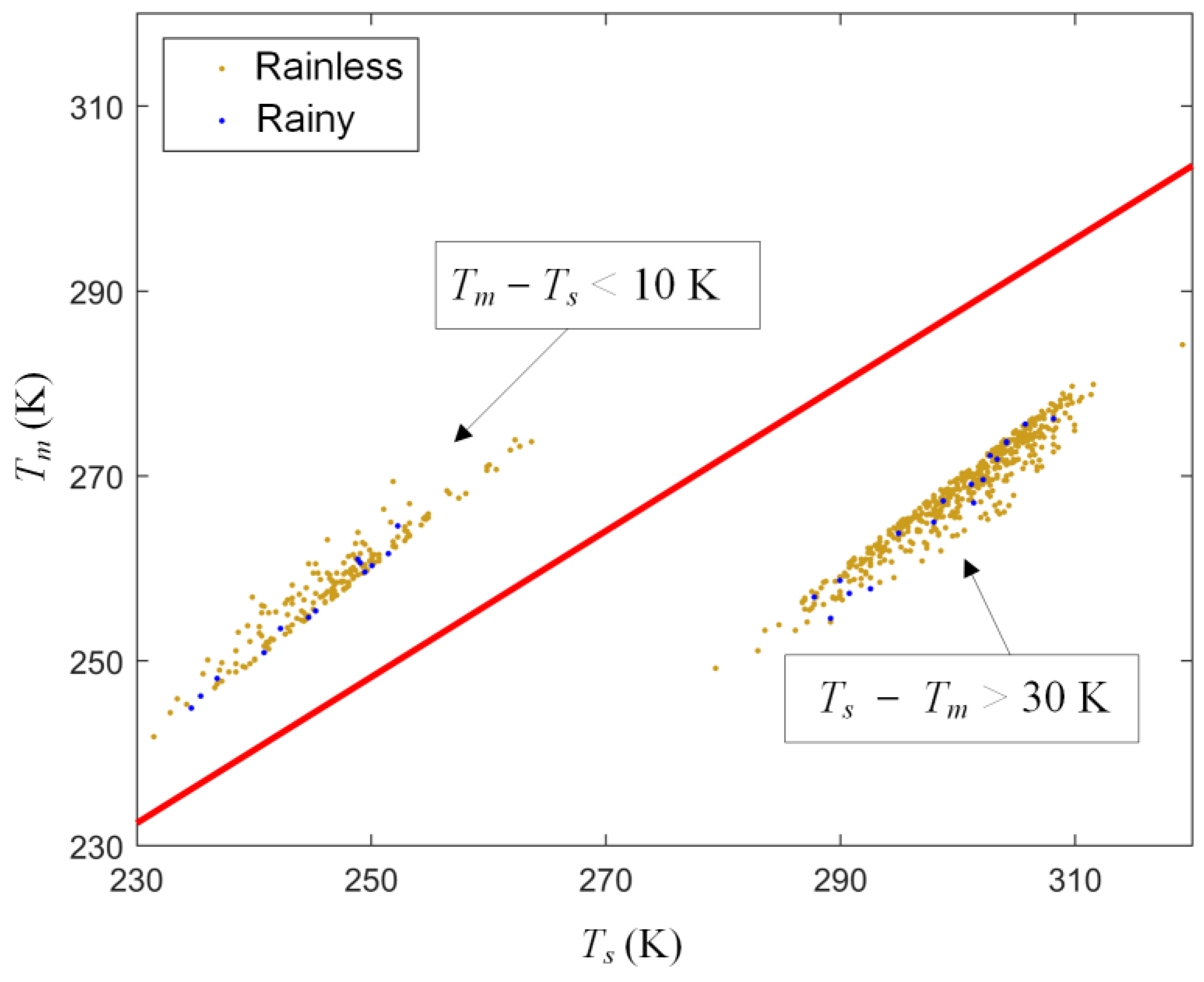
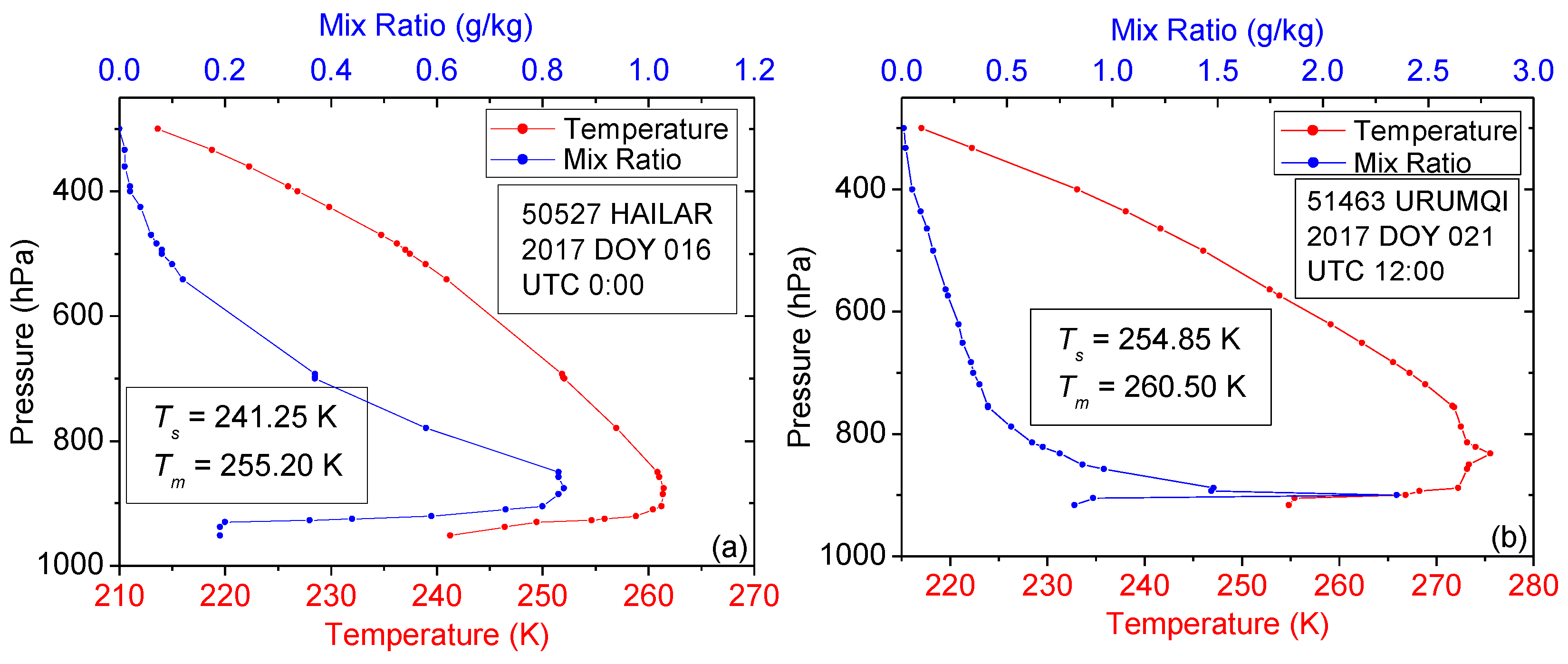
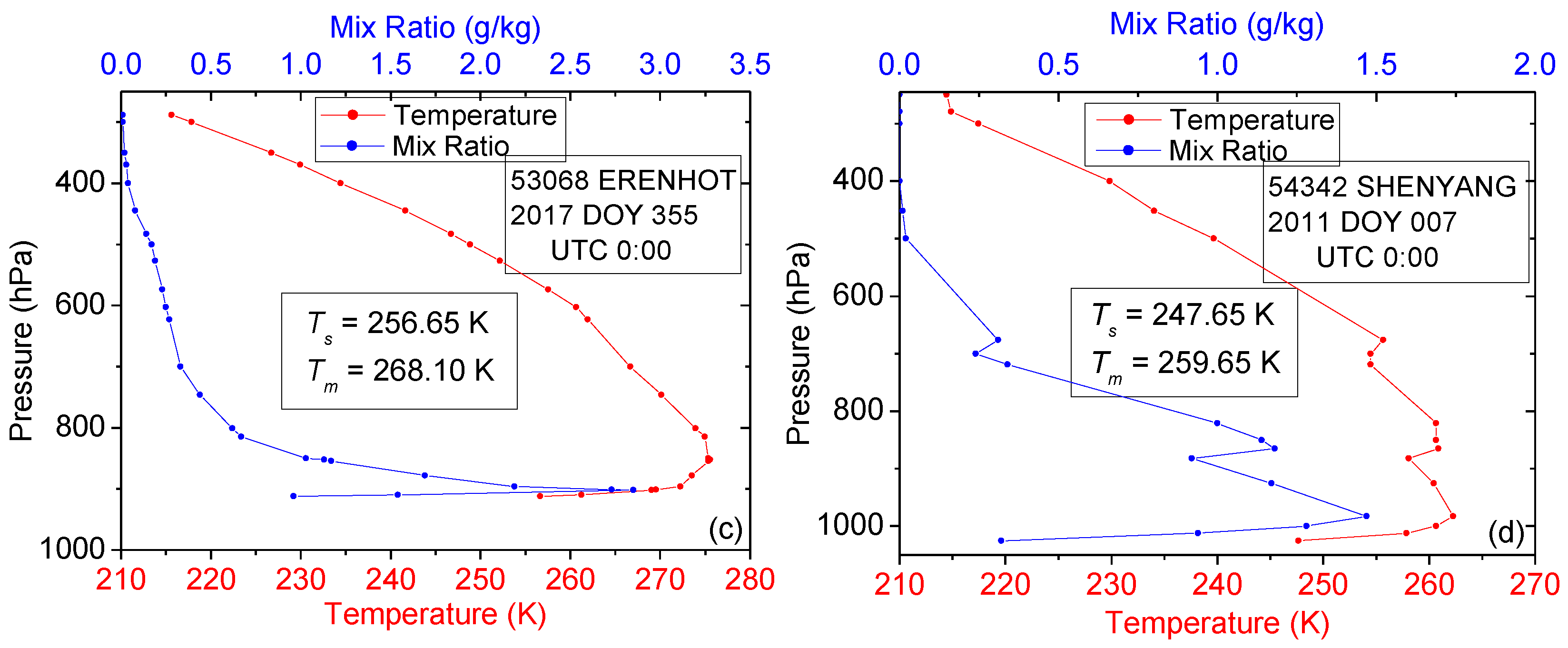
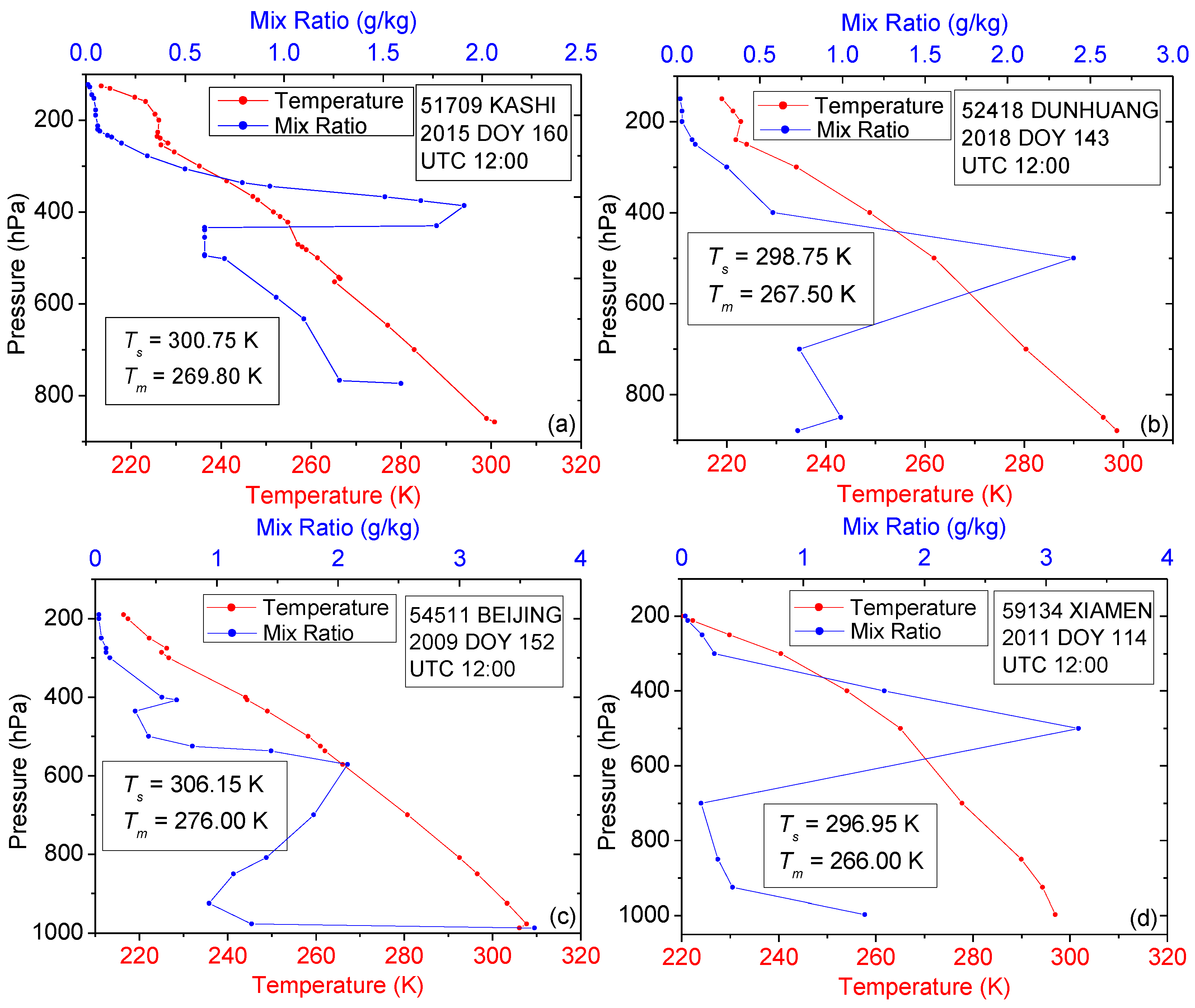
5.3. Weather Conditions Related to Some Specific Data Points
6. Conclusions
Author Contributions
Funding
Data Availability Statement
Acknowledgments
Conflicts of Interest
Appendix A

| Radiosonde Station | Weather- Indenpedent Model | Rainless-Day Model | Rainy-Day Model | ||||||
|---|---|---|---|---|---|---|---|---|---|
| NO. | ID/STN | Lat/Lon | H (m) | a | b | a | b | a | b |
| C1 | C2 | C3 | C4 | C5 | C6 | C7 | C8 | C9 | C10 |
| 1 | 45004 Kings Park | 22.31 114.16 | 66 | 0.57 | 118.16 | 0.62 | 102.43 | 0.49 | 139.34 |
| 2 | 50527 Hailar | 49.21 119.75 | 611 | 0.72 | 69.55 | 0.71 | 72.53 | 0.76 | 56.88 |
| 3 | 50557 Nenjiang | 49.16 125.23 | 243 | 0.77 | 55.79 | 0.75 | 59.88 | 0.81 | 42.53 |
| 4 | 50774 Yichun | 47.71 128.9 | 232 | 0.83 | 38.75 | 0.81 | 44.72 | 0.88 | 25.43 |
| 5 | 50953 Harbin | 45.75 126.76 | 143 | 0.85 | 33.30 | 0.85 | 34.35 | 0.87 | 27.88 |
| 6 | 51076 Altay | 47.73 88.08 | 737 | 0.65 | 90.53 | 0.63 | 96.10 | 0.70 | 75.13 |
| 7 | 51431 Yining | 43.95 81.33 | 664 | 0.65 | 89.68 | 0.61 | 102.63 | 0.74 | 63.36 |
| 8 | 51463 Urumqi | 43.78 87.62 | 919 | 0.60 | 103.13 | 0.57 | 111.42 | 0.64 | 90.21 |
| 9 | 51644 Kuqa | 41.71 82.95 | 1100 | 0.62 | 97.46 | 0.61 | 100.22 | 0.70 | 74.88 |
| 10 | 51709 Kashi | 39.46 75.98 | 1291 | 0.60 | 102.14 | 0.58 | 109.11 | 0.69 | 77.31 |
| 11 | 51777 Ruoqiang | 39.03 88.16 | 889 | 0.58 | 109.52 | 0.57 | 111.79 | 0.67 | 84.11 |
| 12 | 51828 Hotan | 37.13 79.93 | 1375 | 0.61 | 97.69 | 0.60 | 101.21 | 0.69 | 75.81 |
| 13 | 51839 Minfeng | 37.06 82.71 | 1409 | 0.58 | 108.82 | 0.56 | 112.92 | 0.69 | 77.39 |
| 14 | 52203 Hami | 42.81 93.51 | 739 | 0.62 | 98.06 | 0.61 | 99.81 | 0.68 | 79.26 |
| 15 | 52267 Ejin Qi | 41.95 101.06 | 941 | 0.64 | 92.16 | 0.63 | 92.55 | 0.65 | 88.61 |
| 16 | 52323 Maz. Shan | 41.80 97.03 | 1770 | 0.64 | 89.84 | 0.63 | 93.16 | 0.72 | 68.73 |
| 17 | 52418 Dunhuang | 40.15 94.68 | 1140 | 0.59 | 105.47 | 0.58 | 108.71 | 0.71 | 69.68 |
| 18 | 52533 Jiuquan | 39.76 98.48 | 1478 | 0.62 | 96.06 | 0.60 | 101.51 | 0.72 | 67.19 |
| 19 | 52681 Minqin | 38.63 103.08 | 1367 | 0.65 | 89.38 | 0.63 | 93.73 | 0.74 | 61.29 |
| 20 | 52818 Golmud | 36.41 94.90 | 2809 | 0.60 | 98.88 | 0.58 | 104.50 | 0.69 | 74.83 |
| 21 | 52836 Dulan | 36.30 98.10 | 3192 | 0.75 | 57.22 | 0.73 | 63.54 | 0.80 | 46.86 |
| 22 | 52866 Xining | 36.71 101.75 | 2296 | 0.66 | 86.40 | 0.62 | 96.60 | 0.78 | 53.66 |
| 23 | 52983 Yu Zhong | 35.87 104.15 | 1875 | 0.67 | 84.57 | 0.64 | 92.16 | 0.77 | 55.08 |
| 24 | 53068 Erenhot | 43.65 112.00 | 966 | 0.68 | 78.05 | 0.67 | 81.56 | 0.75 | 60.08 |
| 25 | 53463 Hohhot | 40.81 111.68 | 1065 | 0.77 | 54.02 | 0.76 | 57.16 | 0.82 | 38.47 |
| 26 | 53513 Linhe | 40.76 107.40 | 1041 | 0.76 | 59.71 | 0.76 | 59.63 | 0.81 | 45.27 |
| 27 | 53614 Yinchuan | 38.48 106.21 | 1112 | 0.74 | 63.52 | 0.74 | 65.35 | 0.79 | 49.17 |
| 28 | 53772 Taiyuan | 37.78 112.55 | 779 | 0.77 | 54.03 | 0.77 | 55.92 | 0.82 | 41.52 |
| 29 | 53845 Yan An | 36.60 109.50 | 959 | 0.72 | 68.70 | 0.71 | 74.04 | 0.81 | 45.08 |
| 30 | 53915 Pingliang | 35.55 106.66 | 1348 | 0.77 | 56.72 | 0.75 | 61.35 | 0.83 | 38.31 |
| 31 | 54102 Xilin Hot | 43.95 116.06 | 991 | 0.74 | 64.15 | 0.71 | 70.49 | 0.80 | 45.91 |
| 32 | 54135 Tongliao | 43.60 122.26 | 180 | 0.88 | 24.00 | 0.88 | 23.01 | 0.88 | 22.81 |
| 33 | 54161 Changchun | 43.90 125.21 | 238 | 0.87 | 27.66 | 0.87 | 27.91 | 0.88 | 24.66 |
| 34 | 54218 Chifeng | 42.26 118.96 | 572 | 0.85 | 32.86 | 0.84 | 34.16 | 0.86 | 28.66 |
| 35 | 54292 Yanji | 42.88 129.46 | 178 | 0.92 | 13.44 | 0.93 | 12.03 | 0.93 | 11.70 |
| 36 | 54342 Shenyang | 41.76 123.43 | 43 | 0.82 | 41.59 | 0.82 | 41.50 | 0.85 | 31.26 |
| 37 | 54374 Linjiang | 41.71 126.91 | 333 | 0.82 | 41.93 | 0.82 | 44.82 | 0.87 | 27.26 |
| 38 | 54511 Beijing | 39.93 116.28 | 55 | 0.87 | 25.21 | 0.87 | 24.89 | 0.86 | 28.63 |
| 39 | 54662 Dalian | 38.90 121.63 | 97 | 0.96 | 2.57 | 0.97 | -0.20 | 0.93 | 10.08 |
| 40 | 54727 Zhangqiu | 36.70 117.55 | 123 | 0.83 | 37.24 | 0.84 | 36.95 | 0.82 | 40.26 |
| 41 | 54857 Qingdao | 36.06 120.33 | 77 | 0.96 | 3.35 | 0.98 | -3.63 | 0.91 | 17.59 |
| 42 | 55299 Nagqu | 31.48 92.06 | 4508 | 0.67 | 77.83 | 0.55 | 109.67 | 0.75 | 58.35 |
| 43 | 55591 Lhasa | 29.66 91.13 | 3650 | 0.63 | 93.57 | 0.60 | 101.16 | 0.67 | 82.90 |
| 44 | 56029 Yushu | 33.01 97.01 | 3682 | 0.73 | 64.51 | 0.66 | 81.31 | 0.76 | 56.47 |
| 45 | 56080 Hezuo | 35.00 102.90 | 2910 | 0.74 | 63.76 | 0.69 | 76.10 | 0.82 | 42.92 |
| 46 | 56137 Qamdo | 31.15 97.16 | 3307 | 0.70 | 74.10 | 0.65 | 87.75 | 0.71 | 70.39 |
| 47 | 56146 Garze | 31.61 100.00 | 522 | 0.72 | 70.94 | 0.66 | 86.30 | 0.76 | 58.98 |
| 48 | 56187 Wenjiang | 30.70 103.83 | 541 | 0.71 | 72.29 | 0.69 | 80.93 | 0.79 | 48.56 |
| 49 | 56571 Xichang | 27.90 102.26 | 1599 | 0.58 | 110.66 | 0.55 | 121.73 | 0.70 | 75.35 |
| 50 | 56691 Weining | 26.86 104.28 | 2236 | 0.62 | 102.15 | 0.60 | 107.06 | 0.60 | 105.10 |
| 51 | 56739 Tengchong | 25.11 98.48 | 1649 | 0.52 | 130.75 | 0.53 | 127.02 | 0.61 | 102.11 |
| 52 | 56778 Kunming | 25.01 102.68 | 1892 | 0.45 | 148.44 | 0.41 | 161.20 | 0.62 | 99.25 |
| 53 | 56964 Simao | 22.76 100.98 | 1303 | 0.35 | 181.68 | 0.35 | 182.07 | 0.54 | 124.71 |
| 54 | 56985 Mengzi | 23.38 103.38 | 1302 | 0.49 | 138.31 | 0.49 | 141.13 | 0.58 | 113.11 |
| 55 | 57083 Zhengzhou | 34.71 113.65 | 111 | 0.81 | 46.17 | 0.81 | 45.67 | 0.81 | 44.03 |
| 56 | 57127 Hanzhong | 33.06 107.03 | 509 | 0.78 | 54.11 | 0.75 | 61.72 | 0.86 | 27.99 |
| 57 | 57131 Jinghe | 34.43 108.97 | 411 | 0.75 | 60.92 | 0.74 | 64.27 | 0.83 | 39.08 |
| 58 | 57178 Nanyang | 33.03 112.58 | 131 | 0.80 | 48.24 | 0.80 | 48.23 | 0.82 | 42.57 |
| 59 | 57447 Enshi | 30.28 109.46 | 458 | 0.77 | 56.77 | 0.74 | 66.97 | 0.81 | 45.32 |
| 60 | 57461 Yichang | 30.70 111.30 | 134 | 0.80 | 48.09 | 0.81 | 47.18 | 0.80 | 48.65 |
| 61 | 57494 Wuhan | 30.61 114.13 | 23 | 0.75 | 64.14 | 0.75 | 63.45 | 0.74 | 66.97 |
| 62 | 57516 Chongqing | 29.51 106.48 | 260 | 0.81 | 47.57 | 0.77 | 58.23 | 0.83 | 38.87 |
| 63 | 57679 Changsha | 28.20 113.08 | 46 | 0.70 | 78.60 | 0.71 | 76.15 | 0.67 | 85.54 |
| 64 | 57749 Huaihua | 27.56 110.00 | 261 | 0.68 | 83.41 | 0.68 | 83.76 | 0.67 | 86.91 |
| 65 | 57816 Guiyang | 26.48 106.65 | 1222 | 0.62 | 101.20 | 0.64 | 94.89 | 0.59 | 108.71 |
| 66 | 57957 Guilin | 25.33 110.30 | 166 | 0.63 | 99.24 | 0.67 | 87.73 | 0.59 | 110.69 |
| 67 | 57972 Chenzhou | 25.80 113.03 | 185 | 0.62 | 101.09 | 0.64 | 96.77 | 0.60 | 107.27 |
| 68 | 57993 Ganzhou | 25.85 114.95 | 125 | 0.63 | 98.02 | 0.64 | 96.53 | 0.62 | 102.24 |
| 69 | 58027 Xuzhou | 34.28 117.15 | 42 | 0.84 | 37.63 | 0.85 | 35.50 | 0.83 | 38.18 |
| 70 | 58150 Sheyang | 33.76 120.25 | 7 | 0.86 | 32.34 | 0.87 | 27.96 | 0.86 | 29.31 |
| 71 | 58203 Fuyang | 32.86 115.73 | 33 | 0.84 | 37.86 | 0.85 | 35.13 | 0.81 | 44.24 |
| 72 | 58238 Nanjing | 32.00 118.80 | 7 | 0.81 | 44.31 | 0.82 | 42.58 | 0.81 | 46.42 |
| 73 | 58362 Shanghai | 31.40 121.46 | 4 | 0.82 | 42.85 | 0.82 | 41.29 | 0.81 | 43.50 |
| 74 | 58424 Anqing | 30.53 117.05 | 20 | 0.79 | 51.17 | 0.81 | 45.75 | 0.76 | 61.78 |
| 75 | 58457 Hangzhou | 30.23 120.16 | 43 | 0.79 | 50.87 | 0.80 | 49.28 | 0.78 | 53.00 |
| 76 | 58606 Nanchang | 28.60 115.91 | 50 | 0.74 | 67.77 | 0.76 | 61.88 | 0.70 | 78.62 |
| 77 | 58633 Qu Xian | 28.96 118.86 | 71 | 0.73 | 70.12 | 0.72 | 73.11 | 0.74 | 67.51 |
| 78 | 58665 Hongjia | 28.61 121.41 | 2 | 0.78 | 54.31 | 0.80 | 50.01 | 0.77 | 58.05 |
| 79 | 58725 Shaowu | 27.33 117.46 | 219 | 0.69 | 81.32 | 0.69 | 82.75 | 0.71 | 76.99 |
| 80 | 58847 Fuzhou | 26.08 119.28 | 85 | 0.73 | 69.83 | 0.75 | 64.35 | 0.70 | 78.76 |
| 81 | 59134 Xiamen | 24.48 118.08 | 139 | 0.68 | 84.50 | 0.73 | 71.76 | 0.60 | 108.31 |
| 82 | 59211 Baise | 23.90 106.60 | 175 | 0.64 | 95.58 | 0.64 | 97.28 | 0.65 | 93.27 |
| 83 | 59265 Wuzhou | 23.48 111.30 | 120 | 0.58 | 114.12 | 0.62 | 104.13 | 0.54 | 125.68 |
| 84 | 59280 Qing Yuan | 23.66 113.05 | 19 | 0.59 | 111.25 | 0.64 | 97.52 | 0.54 | 126.00 |
| 85 | 59316 Shantou | 23.35 116.66 | 3 | 0.63 | 100.81 | 0.67 | 87.97 | 0.56 | 120.00 |
| 86 | 59431 Nanning | 22.63 108.21 | 126 | 0.54 | 125.08 | 0.58 | 114.61 | 0.50 | 138.79 |
| 87 | 59758 Haikou | 20.03 110.35 | 24 | 0.56 | 121.84 | 0.61 | 108.11 | 0.50 | 137.63 |
| 88 | 59981 Xisha Dao | 16.83 112.33 | 5 | 0.47 | 149.53 | 0.41 | 167.98 | 0.47 | 147.96 |
References
- Bevis, M.; Businger, S.; Herring, T.; Rocken, C.; Anthes, R.; Ware, R. GPS meteorology: Remote sensing of atmospheric water vapor using the Global Positioning System. J. Geophys. Res. 1992, 97, 15787–15801. [Google Scholar] [CrossRef]
- Rocken, C.; Hove, T.; Johnson, J.; Solheim, F.; Ware, R.; Bevis, M.; Chiswell, S.; Businger, S. GPS/STORM—GPS sensing of atmospheric water vapor for meteorology. J. Atmos. Ocean Tech. 1995, 12, 468–478. [Google Scholar] [CrossRef]
- Fang, P.; Bevis, M.; Bock, Y.; Gutman, S.; Wolfe, D. GPS meteorology: Reducing systematic errors in geodetic estimates for zenith delay. Geophys. Res. Lett. 1998, 25, 3583–3586. [Google Scholar] [CrossRef]
- Vaquero-Martinez, J.; Anton, M. Review on the role of GNSS meteorology in monitoring water vapor for atmospheric physics. Remote Sens. 2021, 13, 2287. [Google Scholar] [CrossRef]
- Wang, M. The Assessment and Meteorological Applications of High Spatiotemporal Resolution GPS ZTD/PW Derived by Precise Point Positioning. Ph.D. Dissertation, Tong University, Shanghai, China, 2019. [Google Scholar]
- Zhang, Y.; Cai, C.; Chen, B.; Dai, W. Consistency evaluation of precipitable water vapor derived from ERA5, ERA-Interim, GNSS, and radiosondes over China. Radio Sci. 2019, 54, 561–571. [Google Scholar] [CrossRef]
- Shikhovtsev, A.; Khaikin, V.; Mironov, A.; Kovadlo, P. Statistical Analysis of the Water Vapor Content in North Caucasus and Crimea. Atmos. Ocean Opt. 2022, 35, 168–175. [Google Scholar] [CrossRef]
- Emardson, T.; Elgered, G.; Johansson, J. Three months of continuous monitoring of atmospheric water vapor with a network of Global Positioning System receivers. J. Geophys. Res. 1998, 103, 1807–1820. [Google Scholar] [CrossRef]
- Jin, S.; Luo, O. Variability and climatology of PWV from global 13-year GPS observations. IEEE Trans. Geosci. Remote 2009, 47, 1918–1924. [Google Scholar] [CrossRef]
- Birkenheuer, D.; Gutman, S. A comparison of GOES moisture-derived product and GPS-IPW data during IHOP-2002. J. Atmos. Ocean Tech. 2005, 22, 1838–1845. [Google Scholar] [CrossRef] [Green Version]
- Tan, J.; Chen, B.; Wang, W.; Yu, W.; Dai, W. Evaluating precipitable water vapor products from Fengyun-4A meteorological satellite using radiosonde, GNSS, and ERA5 Data. IEEE Trans. Geosci. Remote 2022, 60, 4106512. [Google Scholar] [CrossRef]
- Adams, D.; Gutman, S.; Holub, K.; Pereira, D. GNSS observations of deep convective time scales in the Amazon. Geophys. Res. Lett. 2013, 40, 2818–2823. [Google Scholar] [CrossRef]
- Huang, L.; Mo, Z.; Xie, S.; Liu, L.; Chen, J.; Kang, C.; Wang, S. Spatiotemporal characteristics of GNSS-derived precipitable water vapor during heavy rainfall events in Guilin, China. Satell. Navig. 2021, 2, 13. [Google Scholar] [CrossRef]
- Shi, C.; Zhou, L.; Fan, L.; Zhang, W.; Cao, Y.; Wang, C.; Xiao, F.; Lv, G.; Liang, H. Analysis of ‘21·7’ extreme rainstorm process in Henan Province using BeiDou/GNSS observation. Chin. J. Geophys. 2022, 65, 186–196. [Google Scholar]
- Moore, A.; Small, I.; Gutman, S.; Bock, Y.; Dumas, J.; Fang, P.; Haase, J.; Jackson, M.; Laber, J. National weather service forecasters use GPS precipitable water vapor for enhanced situational awareness during the southern California summer monsoon. Bull. Am. Meteorol. Soc. 2015, 96, 1867–1877. [Google Scholar] [CrossRef]
- Wang, M.; Wang, J.; Bock, Y.; Liang, H.; Dong, D.; Fang, P. Dynamic mapping of the movement of landfalling atmospheric rivers over southern California with GPS data. Geophys. Res. Lett. 2019, 46, 3551–3559. [Google Scholar] [CrossRef]
- Askne, J.; Nordius, H. Estimation of tropospheric delay for microwaves from surface weather data. Radio Sci. 1987, 22, 379–386. [Google Scholar] [CrossRef]
- Davis, J.; Herring, T.; Shapiro, I.; Rogers, A.; Elgered, G. Geodesy by radio interferometry: Effects of atmospheric modeling errors on estimates of baseline length. Radio Sci. 1985, 20, 1593–1607. [Google Scholar] [CrossRef]
- Bevis, M.; Businger, S.; Chiswell, S.; Herring, T.; Anthes, R.; Rocken, C.; Ware, R. GPS meteorology: Mapping zenith wet delays onto precipitable water. J. Appl. Meteorol. 1994, 33, 379–386. [Google Scholar] [CrossRef]
- Jade, S.; Vijayan, M.; Gaur, V.; Prabhu, T.; Sahu, S. Estimates of precipitable water vapour from GPS data over the Indian subcontinent. J. Atmos. Sol-Terr. Phy. 2005, 67, 623–635. [Google Scholar] [CrossRef]
- Yao, Y.; Zhang, B.; Yue, S.; Xu, C.; Peng, W. Global empirical model for mapping zenith wet delays onto precipitable water. J. Geod. 2013, 87, 439–448. [Google Scholar] [CrossRef]
- Wang, X.; Zhang, K.; Wu, S.; Fan, S.; Cheng, Y. Water vapor weighted mean temperature and its impact on the determination of precipitable water vapor and its linear trend. J. Geophys. Res. 2016, 121, 833–852. [Google Scholar] [CrossRef]
- Mendes, V.; Prates, G.; Santos, L.; Langley, R. An evaluation of the accuracy of models for the determination of the weighted mean temperature of the atmosphere. In Proceedings of the ION 2000 National Technical Meeting, Anaheim, CA, USA, 26–28 January 2000. [Google Scholar]
- Singh, D.; Ghosh, J.; Kashyap, D. Weighted mean temperature model for extra tropical region of India. J. Atmos. Sol-Terr. Phys. 2014, 107, 48–53. [Google Scholar] [CrossRef]
- Huang, L.; Jiang, W.; Liu, L.; Chen, H.; Ye, S. A new global grid model for the determination of atmospheric weighted mean temperature in GPS precipitable water vapor. J. Geod. 2019, 93, 159–176. [Google Scholar] [CrossRef]
- Ross, R.; Rosenfeld, S. Estimating mean weighted temperature of the atmosphere for Global Positioning System applications. J. Geophys. Res. 1997, 102, 21719–21730. [Google Scholar] [CrossRef] [Green Version]
- Wang, J.; Zhang, L.; Dai, A. Global estimates of water-vapor-weighted mean temperature of the atmosphere for GPS applications. J. Geophys. Res. 2005, 110, D21101. [Google Scholar] [CrossRef] [Green Version]
- Baltink, H.; Van Der Marel, H.; Van Der Hoeven, A. Integrated atmospheric water vapor estimates from a regional GPS network. J. Geophys. Res. 2002, 107, ACL 3-1–ACL 3-8. [Google Scholar] [CrossRef] [Green Version]
- Raju, C.; Saha, K.; Thampi, B.; Parameswaran, K. Empirical model for mean temperature for Indian zone and estimation of precipitable water vapor from ground based GPS measurements. Ann. Geophys. 2007, 25, 1935–1948. [Google Scholar] [CrossRef] [Green Version]
- Sapucci, L. Evaluation of modeling water-vapor-weighted mean tropospheric temperature for GNSS-integrated water vapor estimates in Brazil. J. Appl. Meteorol. Clim. 2014, 53, 715–730. [Google Scholar] [CrossRef]
- Zhang, D.; Yuan, L.; Huang, L.; Li, Q. Atmospheric weighted mean temperature modeling for Australia. Geomat. Inf. Sci. Wuhan Univ. 2022, 47, 1146–1153. [Google Scholar]
- Emardson, T.; Derks, H. On the relation between the wet delay and the integrated precipitable water vapour in the European atmosphere. Meteorol. Appl. 2000, 7, 61–68. [Google Scholar] [CrossRef]
- Isioye, O.; Combrinck, L.; Botai, J. Modelling weighted mean temperature in the West African region: Implications for GNSS meteorology. Meteorol. Appl. 2016, 23, 614–632. [Google Scholar] [CrossRef]
- Zhang, S.; Gong, L.; Gao, W.; Zeng, Q.; Xiao, F.; Liu, Z.; Lei, J. A weighted mean temperature model using principal component analysis for Greenland. GPS Solut. 2023, 27, 57. [Google Scholar] [CrossRef]
- Liou, Y.; Teng, Y.; Van Hove, T.; Liljegren, J. Comparison of precipitable water observations in the near tropics by GPS, microwave radiometer, and radiosondes. J. Appl. Meteorol. 2001, 40, 5–15. [Google Scholar] [CrossRef]
- Liu, Y.; Chen, Y.; Liu, J. Determination of weighted mean tropospheric temperature using ground meteorological measurements. Geo-Spat. Inform. Sci. 2001, 4, 14–18. [Google Scholar]
- Wang, X.; Song, L.; Dai, Z.; Cao, Y. Feature analysis of weighted mean temperature Tm in Hong Kong. J. Nanjing Univ. Inf. Sci. Technol. 2011, 3, 47–52. [Google Scholar]
- Böhm, J.; Möller, G.; Schindelegger, M.; Pain, G.; Weber, R. Development of an improved empirical model for slant delays in the troposphere (GPT2w). GPS Solut. 2015, 19, 433–441. [Google Scholar] [CrossRef] [Green Version]
- Landskron, D.; Böhm, J. VMF3/GPT3: Refined discrete and empirical troposphere mapping functions. J. Geod. 2018, 92, 349–360. [Google Scholar] [CrossRef]
- Yao, Y.; Zhu, S.; Yue, S. A globally applicable, season-specific model for estimating the weighted mean temperature of the atmosphere. J. Geod. 2012, 86, 1125–1135. [Google Scholar] [CrossRef]
- Yao, Y.; Xu, C.; Zhang, B.; Cao, N. GTm-III: A new global empirical model for mapping zenith wet delays onto precipitable water vapour. Geophys. J. Int. 2014, 197, 202–212. [Google Scholar] [CrossRef] [Green Version]
- Zhang, H.; Yuan, Y.; Li, W.; Ou, J.; Li, Y.; Zhang, B. GPS PPP-derived precipitable water vapor retrieval based on Tm/Ps from multiple sources of meteorological data sets in China. J. Geophys. Res. 2017, 122, 4165–4183. [Google Scholar] [CrossRef]
- Yang, F.; Guo, J.; Chen, M.; Zhang, D. Establishment and analysis of a refinement method for the GNSS empirical weighted mean temperature model. Acta Geod. Cartogr. Sin. 2022, 51, 2339–2345. [Google Scholar]
- Liang, H.; Cao, Y.; Wan, X.; Xu, Z.; Wang, H.; Hu, H. Meteorological applications of precipitable water vapor measurements retrieved by the national GNSS network of China. Geod. Geodyn. 2015, 6, 135–142. [Google Scholar] [CrossRef] [Green Version]
- Li, J.; Mao, J.; Li, C.; Xia, Q. The approach to remote sensing of water vapor based on GPS and linear regression Tm in eastern region of China. Acta Meteorol. Sin. 1999, 57, 283–292. [Google Scholar]
- Wang, Y.; Liu, L.; Hao, X.; Xiao, J.; Wang, H.; Xu, H. The application study of the GPS meteorology network in Wuhan region. Acta Geod. Cartogr. Sin. 2007, 36, 141–145. [Google Scholar]
- Lv, Y.; Yin, H.; Huang, D.; Wang, X. Modeling of weighted mean atmospheric temperature and application in GPS/PWV of Chengdu region. Sci. Surv. Map 2008, 33, 103–105. [Google Scholar]
- Li, G.; Li, G.; Du, C.; Miao, Z. Weighted mean temperature models for mapping zenith wet delays onto precipitable water in north china. J. Nanjing Inst. Meteorol. 2009, 32, 80–86. [Google Scholar]
- Thayer, G. An improved equation for the radio refractive index of air. Radio Sci. 1974, 9, 803–807. [Google Scholar] [CrossRef]
- Wallace, J.; Hobbs, P. Atmospheric Science: An Introductory Survey, 2nd ed.; Academic Press: New York, NY, USA, 2006; p. 80. [Google Scholar]
- Wessel, P.; Luis, J.; Uieda, L.; Scharroo, R.; Wobbe, F.; Smith, W.; Tian, D. The Generic Mapping Tools version 6. Geochem. Geophys. Geosyst. 2019, 20, 5556–5564. [Google Scholar] [CrossRef] [Green Version]
- Vihma, T.; Kilpeläinen, T.; Manninen, M.; Sjöblom, A.; Jakobson, E.; Palo, T.; Jaagus, J.; Maturilli, M. Characteristics of temperature and humidity inversions and low-level jets over Svalbard fjords in spring. Adv. Meteorol. 2011, 2011, 486807. [Google Scholar] [CrossRef]
- Yao, Y.; Zhang, B.; Xu, C.; Chen, J. Analysis of the global Tm-Ts correlation and establishment of the latitude-related linear model. Chin. Sci. Bull. 2014, 59, 2340–2347. [Google Scholar] [CrossRef]


Disclaimer/Publisher’s Note: The statements, opinions and data contained in all publications are solely those of the individual author(s) and contributor(s) and not of MDPI and/or the editor(s). MDPI and/or the editor(s) disclaim responsibility for any injury to people or property resulting from any ideas, methods, instructions or products referred to in the content. |
© 2023 by the authors. Licensee MDPI, Basel, Switzerland. This article is an open access article distributed under the terms and conditions of the Creative Commons Attribution (CC BY) license (https://creativecommons.org/licenses/by/4.0/).
Share and Cite
Wang, M.; Chen, J.; Han, J.; Zhang, Y.; Fan, M.; Yu, M.; Sun, C.; Xie, T. Region-Specific and Weather-Dependent Characteristics of the Relation between GNSS-Weighted Mean Temperature and Surface Temperature over China. Remote Sens. 2023, 15, 1538. https://doi.org/10.3390/rs15061538
Wang M, Chen J, Han J, Zhang Y, Fan M, Yu M, Sun C, Xie T. Region-Specific and Weather-Dependent Characteristics of the Relation between GNSS-Weighted Mean Temperature and Surface Temperature over China. Remote Sensing. 2023; 15(6):1538. https://doi.org/10.3390/rs15061538
Chicago/Turabian StyleWang, Minghua, Junping Chen, Jie Han, Yize Zhang, Mengtian Fan, Miao Yu, Chengzhi Sun, and Tao Xie. 2023. "Region-Specific and Weather-Dependent Characteristics of the Relation between GNSS-Weighted Mean Temperature and Surface Temperature over China" Remote Sensing 15, no. 6: 1538. https://doi.org/10.3390/rs15061538