
Forest Emissions Reduction Assessment Using Optical Satellite Imagery and Space LiDAR Fusion for Carbon Stock Estimation


Abstract
:1. Introduction
2. Data and Methods
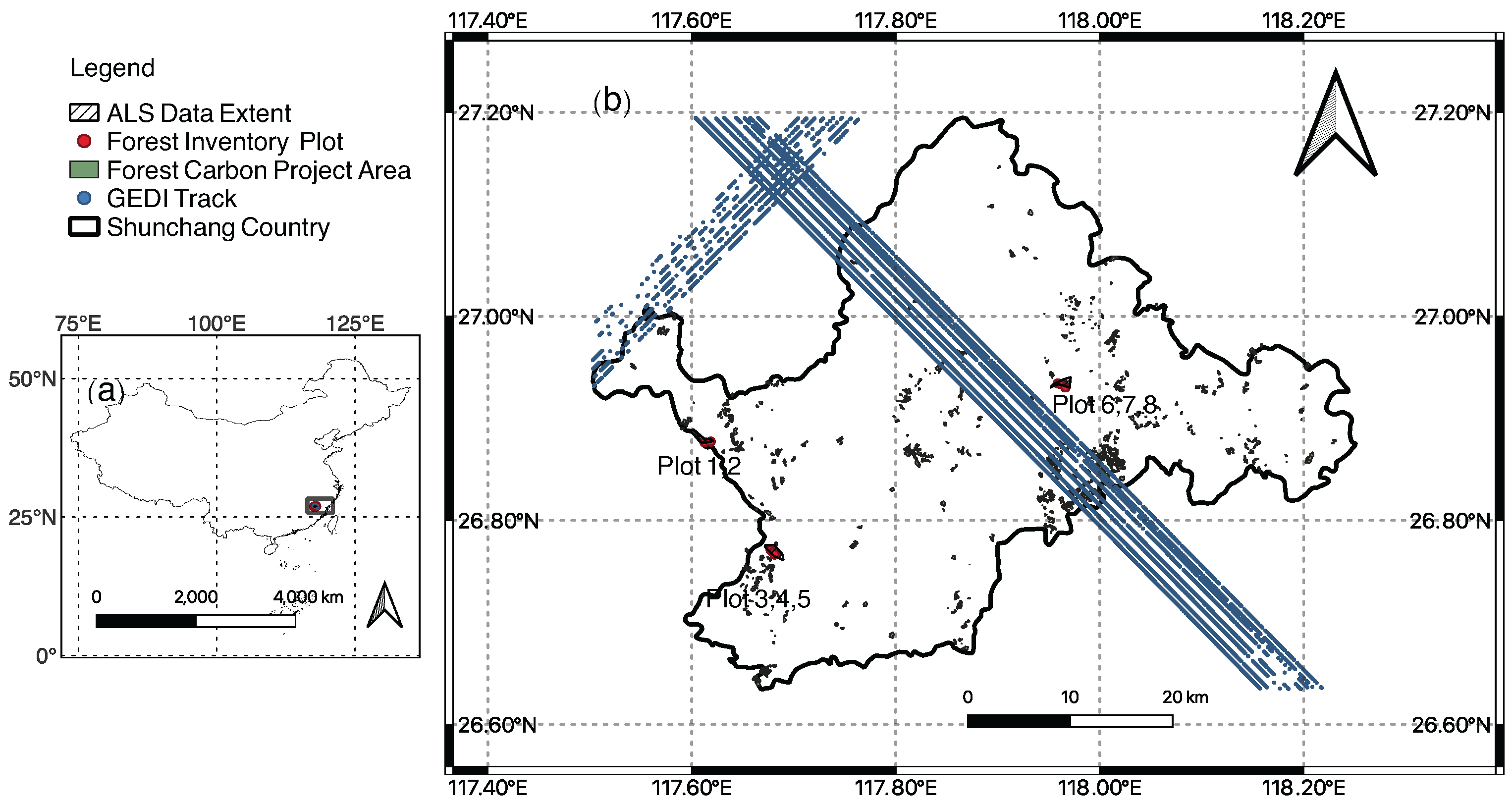
2.1. Research Area
2.2. Field Data and Biomass Allometry
2.3. ALS Data
2.4. Optical Satellite Imagery and Space LiDAR Data
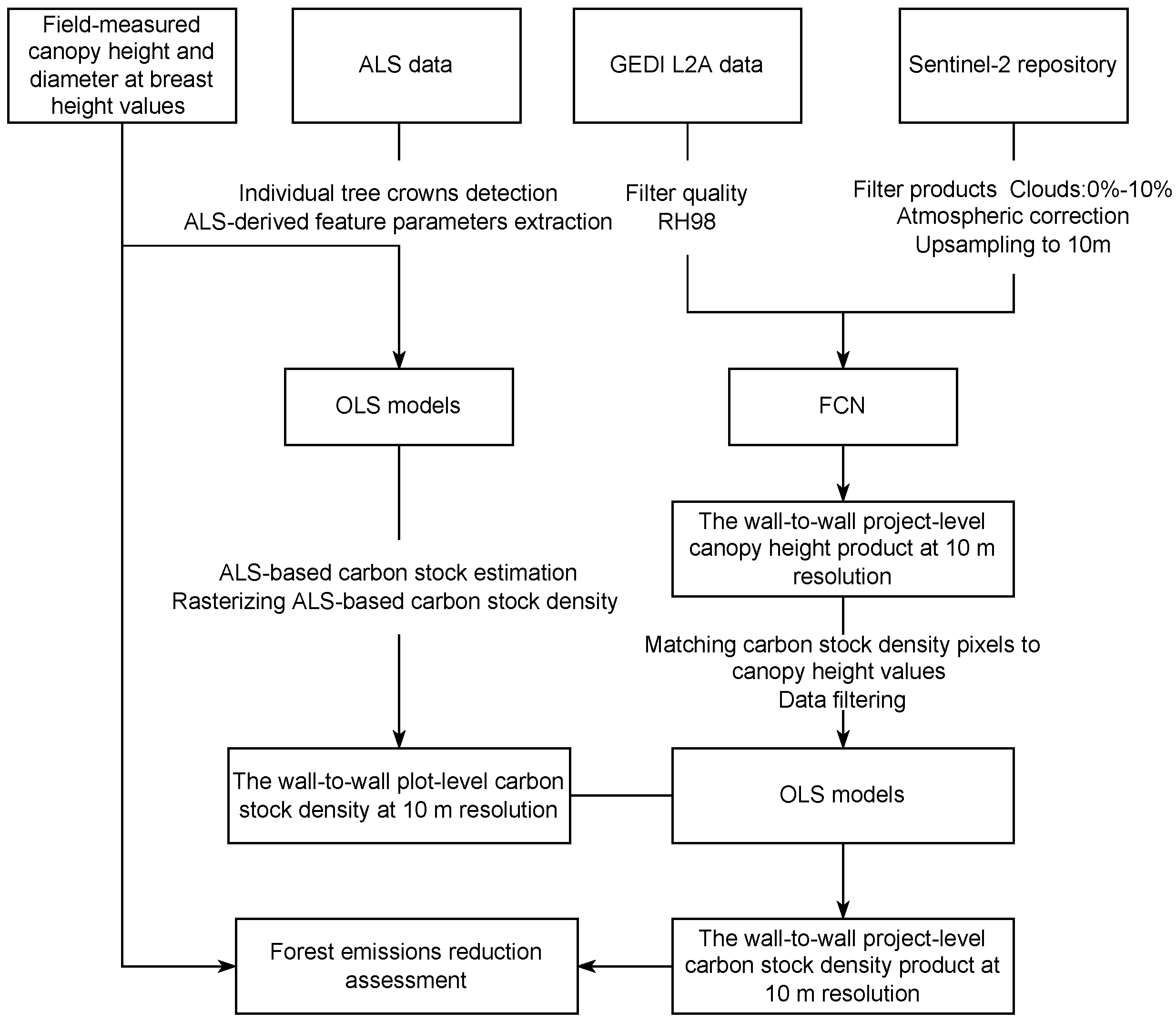
2.5. LiDAR Data Pre-Processing and Individual Tree Segmentation
2.6. Estimating Plot-Level carbon from ALS Data
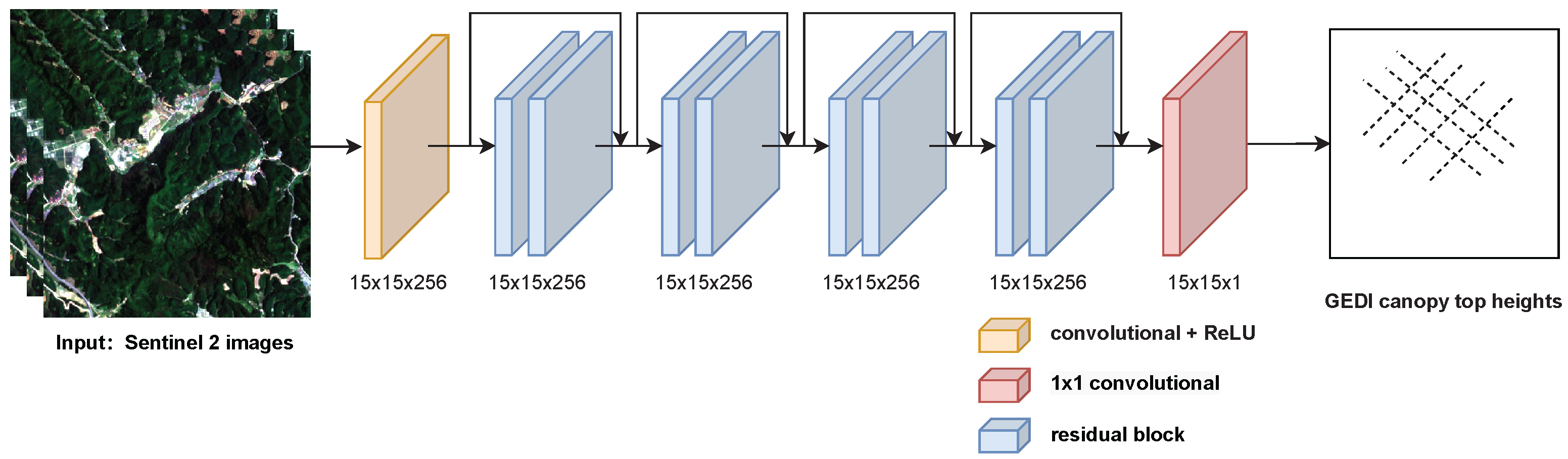
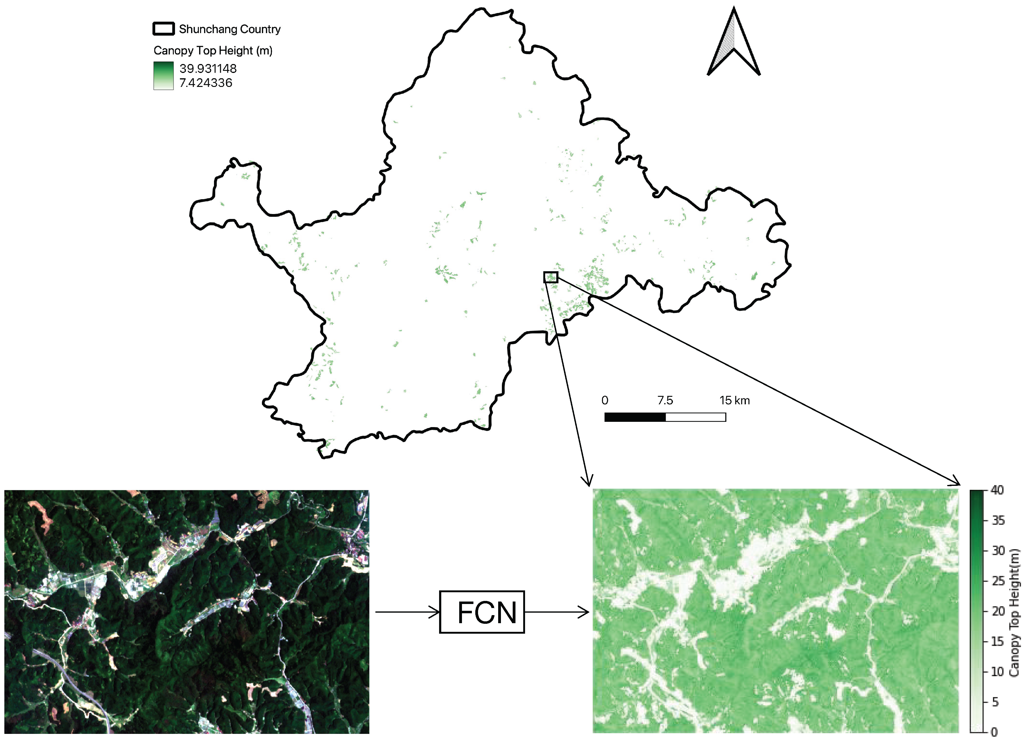
2.7. Sentinel-2 GEDI Data Fusion for Dense Canopy Top Height Mapping
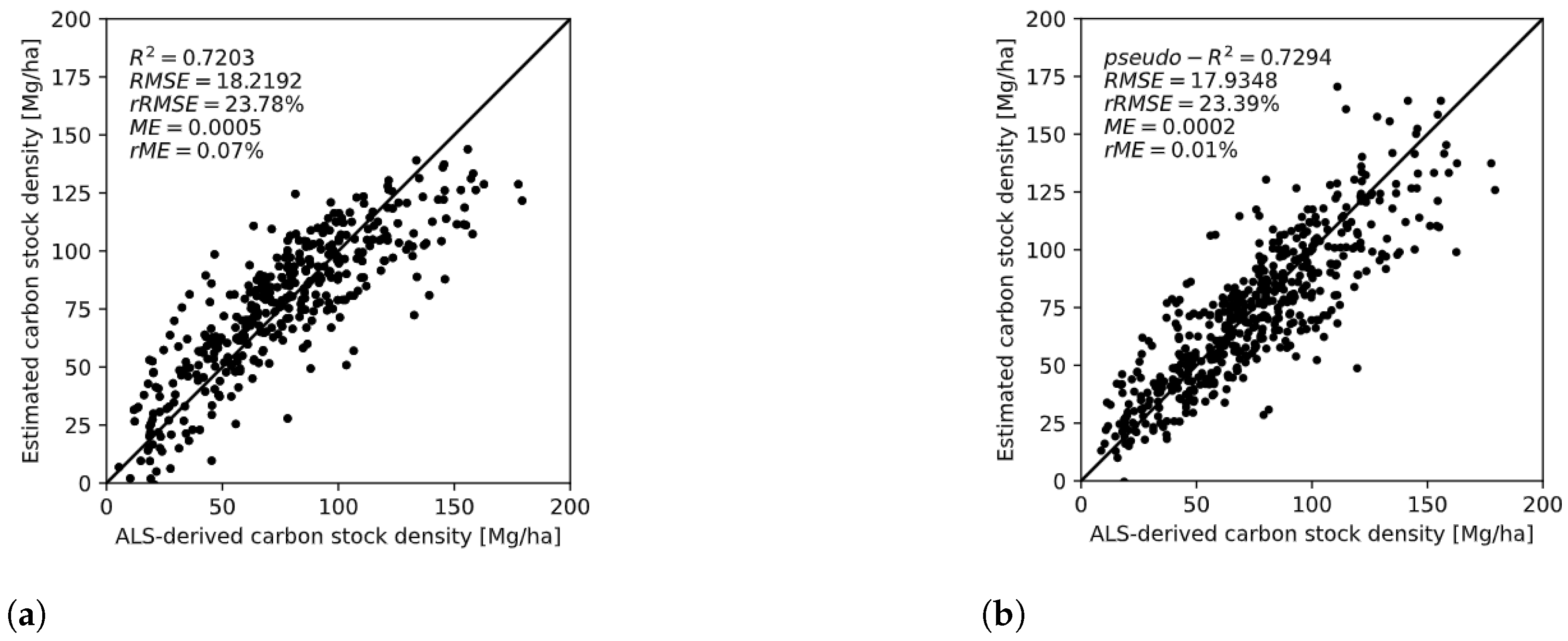
2.8. Estimating Carbon Stock Density from Dense Canopy Top Height and ALS Data
2.9. Project-Level Carbon Stock Assessment
3. Results
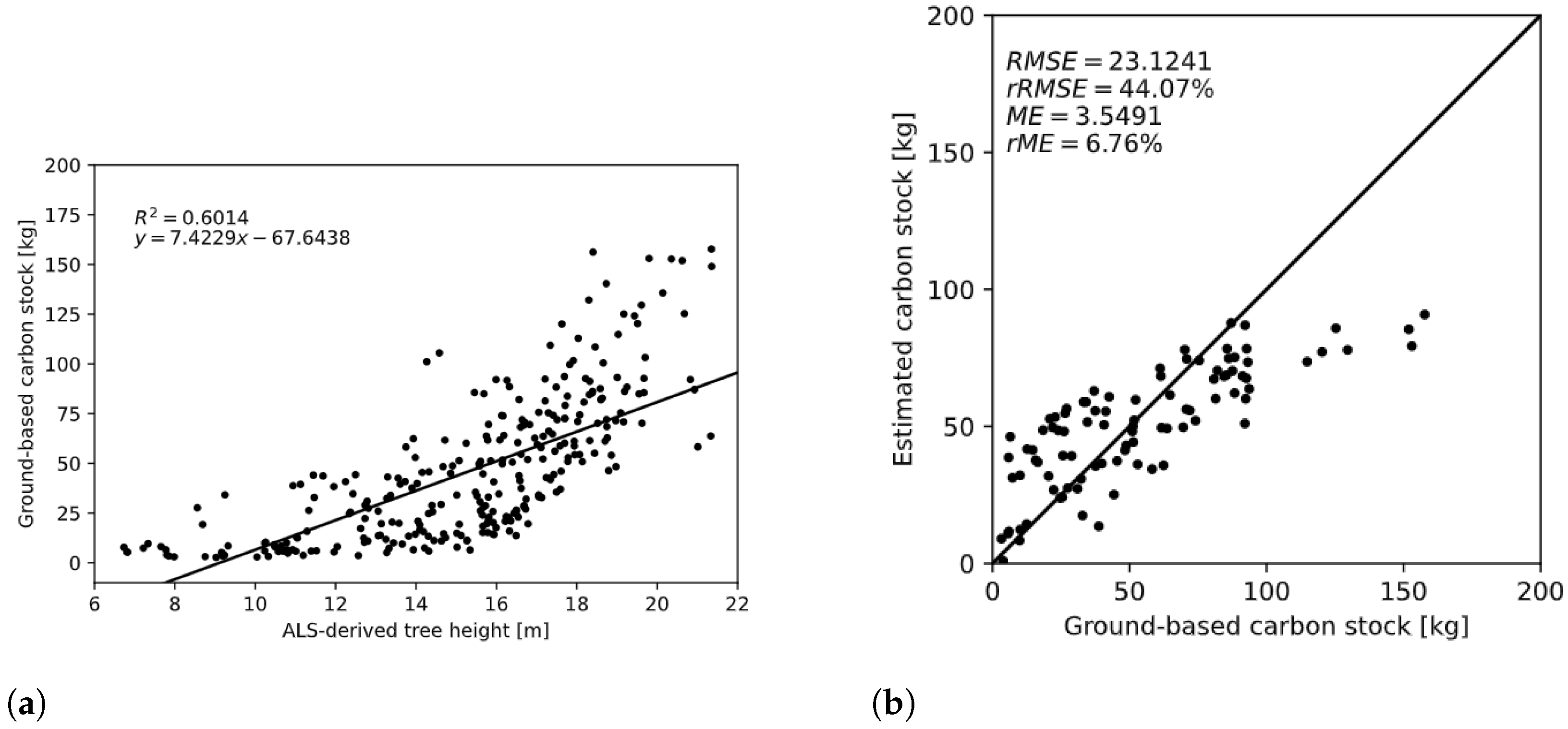
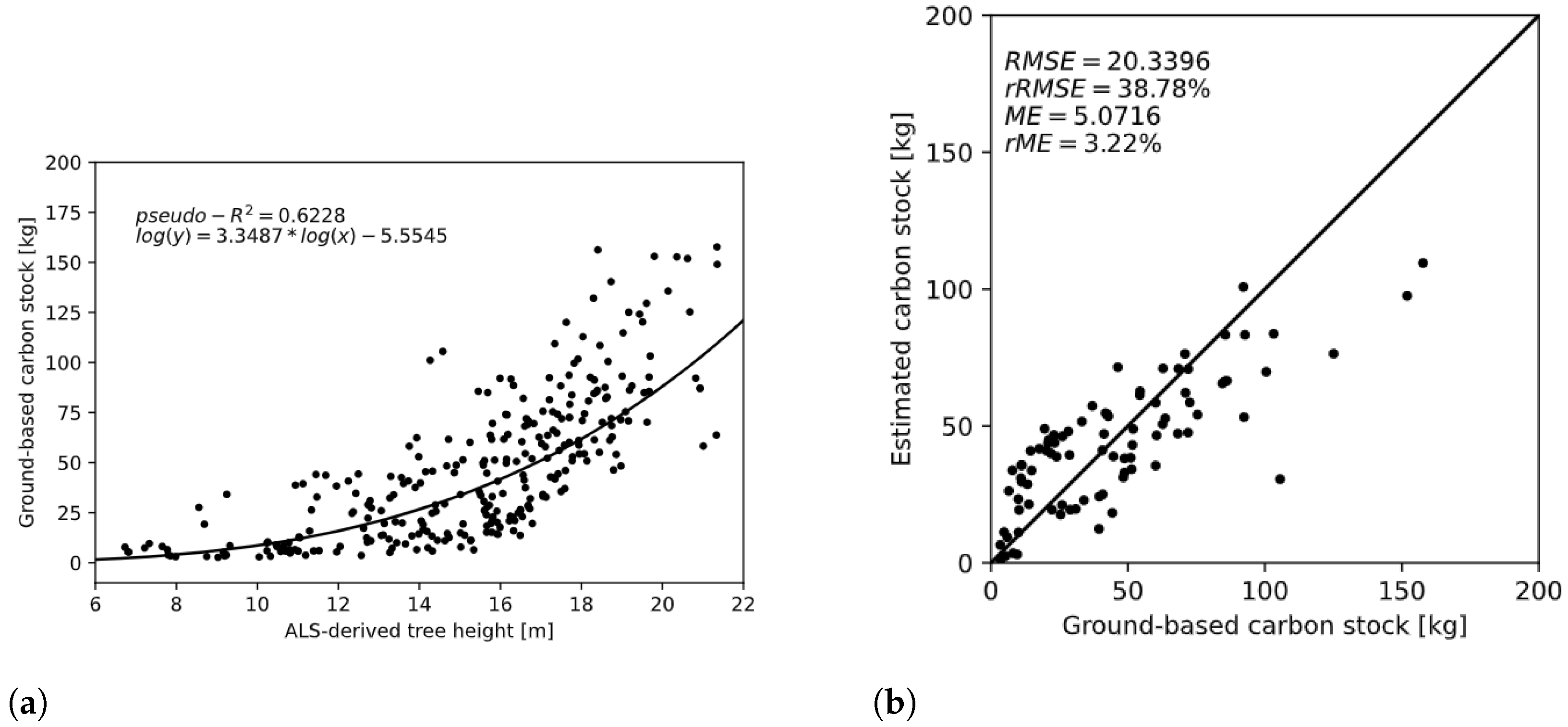
3.1. Performance of Tree-Centric ALS-Based Carbon Stock Estimation
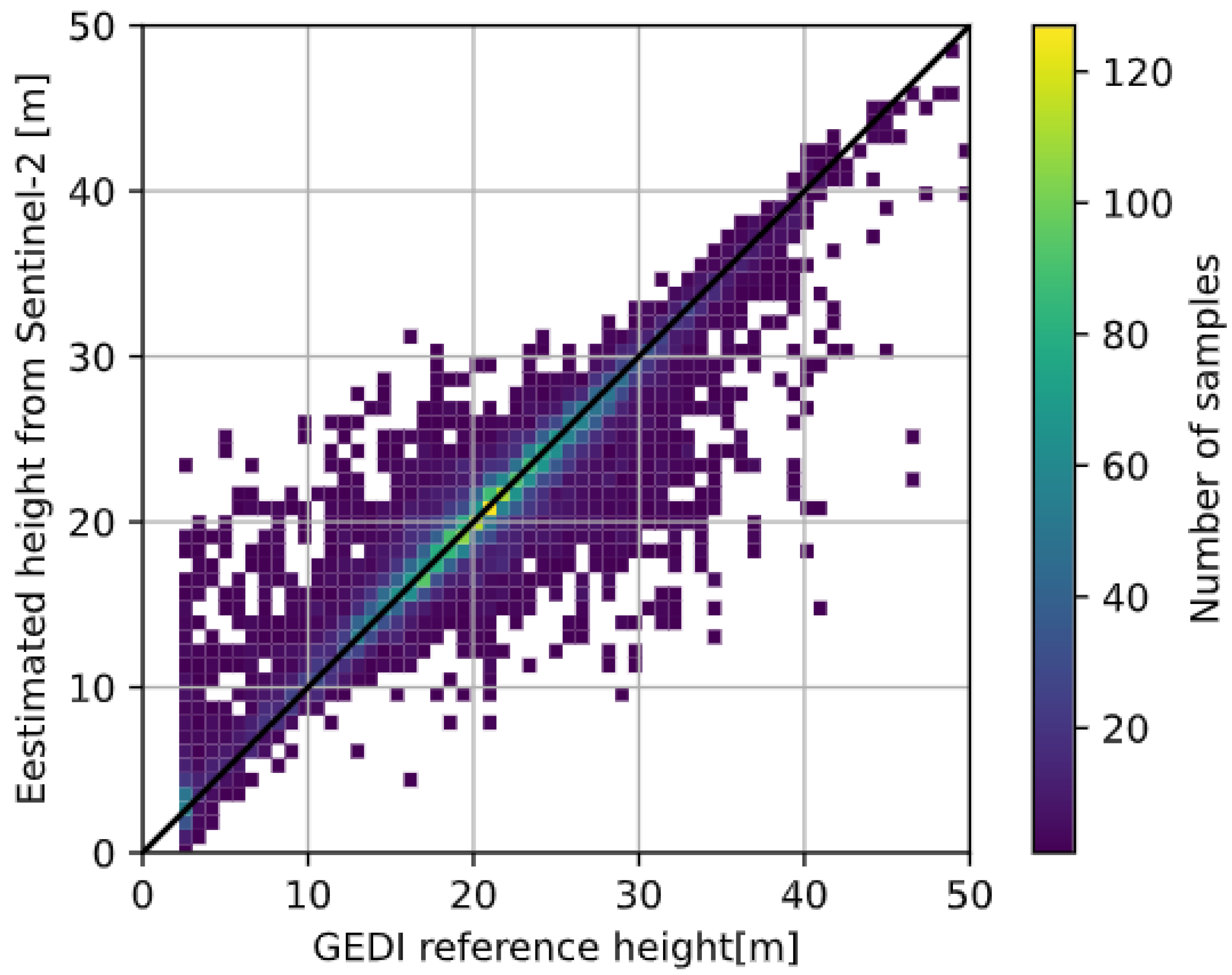
3.2. Performance of Dense Canopy Top Height Mapping
3.3. Performance of Project Emissions Reduction Estimation
4. Discussion
4.1. Benefits of Optical Satellite Imagery and Space LiDAR Data Fusion
4.2. Comparison with Other Canopy Height and Biomass Carbon Stock Estimation Models
4.3. Major Challenges from Field Data Collection to Satellite-Based Project-Level Carbon Stock Mapping
5. Conclusions
Author Contributions
Funding
Data Availability Statement
Conflicts of Interest
References
- Harris, N.L.; Gibbs, D.A.; Baccini, A.; Birdsey, R.A.; De Bruin, S.; Farina, M.; Fatoyinbo, L.; Hansen, M.C.; Herold, M.; Houghton, R.A.; et al. Global maps of twenty-first century forest carbon fluxes. Nat. Clim. Chang. 2021, 11, 234–240. [Google Scholar] [CrossRef]
- Cook-Patton, S.C.; Leavitt, S.M.; Gibbs, D.; Harris, N.L.; Lister, K.; Anderson-Teixeira, K.J.; Briggs, R.D.; Chazdon, R.L.; Crowther, T.W.; Ellis, P.W.; et al. Mapping carbon accumulation potential from global natural forest regrowth. Nature 2020, 585, 545–550. [Google Scholar] [CrossRef]
- Lee, D.H.; Kim, D.H.; Kim, S.I. Characteristics of forest carbon credit transactions in the voluntary carbon market. Clim. Policy 2018, 18, 235–245. [Google Scholar] [CrossRef]
- Qin, S.; Nie, S.; Guan, Y.; Zhang, D.; Wang, C.; Zhang, X. Forest emissions reduction assessment using airborne LiDAR for biomass estimation. Resour. Conserv. Recycl. 2022, 181, 106224. [Google Scholar] [CrossRef]
- Drake, J.B.; Dubayah, R.O.; Knox, R.G.; Clark, D.B.; Blair, J.B. Sensitivity of large-footprint lidar to canopy structure and biomass in a neotropical rainforest. Remote Sens. Environ. 2002, 81, 378–392. [Google Scholar] [CrossRef]
- Popescu, S.C. Estimating biomass of individual pine trees using airborne lidar. Biomass Bioenergy 2007, 31, 646–655. [Google Scholar] [CrossRef]
- Chen, Q.; Qi, C. Lidar remote sensing of vegetation biomass. Remote Sens. Nat. Resour. 2013, 399, 399–420. [Google Scholar]
- Lu, D.; Chen, Q.; Wang, G.; Liu, L.; Li, G.; Moran, E. A survey of remote sensing-based aboveground biomass estimation methods in forest ecosystems. Int. J. Digit. Earth 2016, 9, 63–105. [Google Scholar] [CrossRef]
- Rodríguez-Veiga, P.; Wheeler, J.; Louis, V.; Tansey, K.; Balzter, H. Quantifying forest biomass carbon stocks from space. Curr. For. Rep. 2017, 3, 1–18. [Google Scholar] [CrossRef] [Green Version]
- Saatchi, S.S.; Harris, N.L.; Brown, S.; Lefsky, M.; Mitchard, E.T.; Salas, W.; Zutta, B.R.; Buermann, W.; Lewis, S.L.; Hagen, S.; et al. Benchmark map of forest carbon stocks in tropical regions across three continents. Proc. Natl. Acad. Sci. USA 2011, 108, 9899–9904. [Google Scholar] [CrossRef] [Green Version]
- Baccini, A.; Goetz, S.J.; Walker, W.S.; Laporte, N.T.; Sun, M.; Sulla-Menashe, D.; Hackler, J.; Beck, P.S.A.; Dubayah, R.; Friedl, M.A.; et al. Estimated carbon dioxide emissions from tropical deforestation improved by carbon-density maps. Nat. Clim. Chang. 2012, 2, 182–185. [Google Scholar] [CrossRef]
- Huang, H.; Liu, C.; Wang, X.; Zhou, X.; Gong, P. Integration of multi-resource remotely sensed data and allometric models for forest aboveground biomass estimation in China. Remote Sens. Environ. 2019, 221, 225–234. [Google Scholar] [CrossRef]
- Zhang, R.; Zhou, X.; Ouyang, Z.; Avitabile, V.; Qi, J.; Chen, J.; Giannico, V. Estimating aboveground biomass in subtropical forests of China by integrating multisource remote sensing and ground data. Remote Sens. Environ. 2019, 232, 111341. [Google Scholar] [CrossRef]
- Campbell, M.J.; Dennison, P.E.; Kerr, K.L.; Brewer, S.C.; Anderegg, W.R. Scaled biomass estimation in woodland ecosystems: Testing the individual and combined capacities of satellite multispectral and lidar data. Remote Sens. Environ. 2021, 262, 112511. [Google Scholar] [CrossRef]
- Nandy, S.; Srinet, R.; Padalia, H. Mapping forest height and aboveground biomass by integrating ICESat-2, Sentinel-1 and Sentinel-2 data using Random Forest algorithm in northwest Himalayan foothills of India. Geophys. Res. Lett. 2021, 48, e2021GL093799. [Google Scholar] [CrossRef]
- Lang, N.; Jetz, W.; Schindler, K.; Wegner, J.D. A high-resolution canopy height model of the Earth. arXiv 2022, arXiv:2204.08322. [Google Scholar]
- Guerra-Hernández, J.; Narine, L.L.; Pascual, A.; Gonzalez-Ferreiro, E.; Botequim, B.; Malambo, L.; Neuenschwander, A.; Popescu, S.C.; Godinho, S. Aboveground biomass mapping by integrating ICESat-2, SENTINEL-1, SENTINEL-2, ALOS2/PALSAR2, and topographic information in Mediterranean forests. GIScience Remote Sens. 2022, 59, 1509–1533. [Google Scholar] [CrossRef]
- Jiang, F.; Deng, M.; Tang, J.; Fu, L.; Sun, H. Integrating spaceborne LiDAR and Sentinel-2 images to estimate forest aboveground biomass in Northern China. Carbon Balance Manag. 2022, 17, 1–13. [Google Scholar] [CrossRef]
- Shendryk, Y. Fusing GEDI with earth observation data for large area aboveground biomass mapping. Int. J. Appl. Earth Obs. Geoinf. 2022, 115, 103108. [Google Scholar] [CrossRef]
- Santoro, M.; Cartus, O.; Wegmüller, U.; Besnard, S.; Carvalhais, N.; Araza, A.; Herold, M.; Liang, J.; Cavlovic, J.; Engdahl, M.E. Global estimation of aboveground biomass from spaceborne C-band scatterometer observations aided by LiDAR metrics of vegetation structure. Remote Sens. Environ. 2022, 279, 113114. [Google Scholar] [CrossRef]
- Réjou-Méchain, M.; Barbier, N.; Couteron, P.; Ploton, P.; Vincent, G.; Herold, M.; Mermoz, S.; Saatchi, S.; Chave, J.; De Boissieu, F.; et al. Upscaling forest biomass from field to satellite measurements: Sources of errors and ways to reduce them. Surv. Geophys. 2019, 40, 881–911. [Google Scholar] [CrossRef]
- Chave, J.; Andalo, C.; Brown, S.; Cairns, M.A.; Chambers, J.Q.; Eamus, D.; Fölster, H.; Fromard, F.; Higuchi, N.; Kira, T.; et al. Tree allometry and improved estimation of carbon stocks and balance in tropical forests. Oecologia 2005, 145, 87–99. [Google Scholar] [CrossRef] [PubMed]
- Penman, J.; Gytarsky, M.; Hiraishi, T.; Krug, T.; Kruger, D.; Pipatti, R.; Buendia, L.; Miwa, K.; Ngara, T.; Tanabe, K.; et al. Good Practice Guidance for Land Use, Land-Use Change and Forestry; IPCC: Geneva, Switzerland, 2003. [Google Scholar]
- Dubayah, R.; Armston, J.; Kellner, J.; Duncanson, L.; Healey, S.; Patterson, P.; Hancock, S.; Tang, H.; Bruening, J.; Hofton, M.; et al. GEDI L4A Footprint Level Aboveground Biomass Density; Version 2.1; ORNL DAAC: Oak Ridge, TN, USA, 2022. [Google Scholar]
- Blair, J.B.; Hofton, M.A. Modeling laser altimeter return waveforms over complex vegetation using high-resolution elevation data. Geophys. Res. Lett. 1999, 26, 2509–2512. [Google Scholar] [CrossRef]
- Chave, J.; Davies, S.J.; Phillips, O.L.; Lewis, S.L.; Sist, P.; Schepaschenko, D.; Armston, J.; Baker, T.R.; Coomes, D.; Disney, M.; et al. Ground data are essential for biomass remote sensing missions. Surv. Geophys. 2019, 40, 863–880. [Google Scholar] [CrossRef]
- Zhang, K.; Chen, S.C.; Whitman, D.; Shyu, M.L.; Yan, J.; Zhang, C. A progressive morphological filter for removing nonground measurements from airborne LIDAR data. IEEE Trans. Geosci. Remote Sens. 2003, 41, 872–882. [Google Scholar] [CrossRef] [Green Version]
- Hyyppa, J.; Kelle, O.; Lehikoinen, M.; Inkinen, M. A segmentation-based method to retrieve stem volume estimates from 3-D tree height models produced by laser scanners. IEEE Trans. Geosci. Remote Sens. 2001, 39, 969–975. [Google Scholar] [CrossRef]
- Dalponte, M.; Coomes, D.A. Tree-centric mapping of forest carbon density from airborne laser scanning and hyperspectral data. Methods Ecol. Evol. 2016, 7, 1236–1245. [Google Scholar] [CrossRef] [Green Version]
- Long, J.; Shelhamer, E.; Darrell, T. Fully convolutional networks for semantic segmentation. In Proceedings of the IEEE Conference on Computer Vision and Pattern Recognition, Boston, MA, USA, 7–12 June 2015; pp. 3431–3440. [Google Scholar]
- He, K.; Zhang, X.; Ren, S.; Sun, J. Deep residual learning for image recognition. In Proceedings of the IEEE Conference on Computer Vision and Pattern Recognition, Las Vegas, NV, USA, 26 June–1 July 2016; pp. 770–778. [Google Scholar]
- Kingma, D.P.; Ba, J. Adam: A method for stochastic optimization. arXiv 2014, arXiv:1412.6980. [Google Scholar]
- Asner, G.P.; Mascaro, J. Mapping tropical forest carbon: Calibrating plot estimates to a simple LiDAR metric. Remote Sens. Environ. 2014, 140, 614–624. [Google Scholar] [CrossRef]
- Li, W.; Niu, Z.; Shang, R.; Qin, Y.; Wang, L.; Chen, H. High-resolution mapping of forest canopy height using machine learning by coupling ICESat-2 LiDAR with Sentinel-1, Sentinel-2 and Landsat-8 data. Int. J. Appl. Earth Obs. Geoinf. 2020, 92, 102163. [Google Scholar] [CrossRef]
- Sothe, C.; Gonsamo, A.; Lourenço, R.B.; Kurz, W.A.; Snider, J. Spatially Continuous Mapping of Forest Canopy Height in Canada by Combining GEDI and ICESat-2 with PALSAR and Sentinel. Remote Sens. 2022, 14, 5158. [Google Scholar] [CrossRef]
- Torres de Almeida, C.; Gerente, J.; Rodrigo dos Prazeres Campos, J.; Caruso Gomes Junior, F.; Providelo, L.A.; Marchiori, G.; Chen, X. Canopy Height Mapping by Sentinel 1 and 2 Satellite Images, Airborne LiDAR Data, and Machine Learning. Remote Sens. 2022, 14, 4112. [Google Scholar] [CrossRef]
- Gupta, R.; Sharma, L.K. Mixed tropical forests canopy height mapping from spaceborne LiDAR GEDI and multisensor imagery using machine learning models. Remote Sens. Appl. Soc. Environ. 2022, 27, 100817. [Google Scholar] [CrossRef]
- Lang, N.; Schindler, K.; Wegner, J.D. Country-wide high-resolution vegetation height mapping with Sentinel-2. Remote Sens. Environ. 2019, 233, 111347. [Google Scholar] [CrossRef] [Green Version]
- Duncanson, L.; Kellner, J.R.; Armston, J.; Dubayah, R.; Minor, D.M.; Hancock, S.; Healey, S.P.; Patterson, P.L.; Saarela, S.; Marselis, S.; et al. Aboveground biomass density models for NASA’s Global Ecosystem Dynamics Investigation (GEDI) lidar mission. Remote Sens. Environ. 2022, 270, 112845. [Google Scholar] [CrossRef]
- Swetnam, T.L.; Brooks, P.D.; Barnard, H.R.; Harpold, A.A.; Gallo, E.L. Topographically driven differences in energy and water constrain climatic control on forest carbon sequestration. Ecosphere 2017, 8, e01797. [Google Scholar] [CrossRef] [Green Version]
- Torresan, C.; Berton, A.; Carotenuto, F.; Chiavetta, U.; Miglietta, F.; Zaldei, A.; Gioli, B. Development and performance assessment of a low-cost UAV laser scanner system (LasUAV). Remote Sens. 2018, 10, 1094. [Google Scholar] [CrossRef] [Green Version]
- Schwartz, M.; Ciais, P.; Ottlé, C.; De Truchis, A.; Vega, C.; Fayad, I.; Brandt, M.; Fensholt, R.; Baghdadi, N.; Morneau, F.; et al. High-resolution canopy height map in the Landes forest (France) based on GEDI, Sentinel-1, and Sentinel-2 data with a deep learning approach. arXiv 2022, arXiv:2212.10265. [Google Scholar]
- Kanmegne Tamga, D.; Latifi, H.; Ullmann, T.; Baumhauer, R.; Bayala, J.; Thiel, M. Estimation of Aboveground Biomass in Agroforestry Systems over Three Climatic Regions in West Africa Using Sentinel-1, Sentinel-2, ALOS, and GEDI Data. Sensors 2022, 23, 349. [Google Scholar] [CrossRef]
- Chen, L.; Ren, C.; Bao, G.; Zhang, B.; Wang, Z.; Liu, M.; Man, W.; Liu, J. Improved object-based estimation of forest aboveground biomass by integrating LiDAR data from GEDI and ICESat-2 with multi-sensor images in a heterogeneous mountainous region. Remote Sens. 2022, 14, 2743. [Google Scholar] [CrossRef]
- Heurich, M. Automatic recognition and measurement of single trees based on data from airborne laser scanning over the richly structured natural forests of the Bavarian Forest National Park. For. Ecol. Manag. 2008, 255, 2416–2433. [Google Scholar] [CrossRef]
- Aubry-Kientz, M.; Dutrieux, R.; Ferraz, A.; Saatchi, S.; Hamraz, H.; Williams, J.; Coomes, D.; Piboule, A.; Vincent, G. A comparative assessment of the performance of individual tree crowns delineation algorithms from ALS data in tropical forests. Remote Sens. 2019, 11, 1086. [Google Scholar] [CrossRef] [Green Version]
- Xu, W.; Deng, S.; Liang, D.; Cheng, X. A crown morphology-based approach to individual tree detection in subtropical mixed broadleaf urban forests using UAV LiDAR data. Remote Sens. 2021, 13, 1278. [Google Scholar] [CrossRef]
- Zhang, C.; Zhou, Y.; Qiu, F. Individual tree segmentation from LiDAR point clouds for urban forest inventory. Remote Sens. 2015, 7, 7892–7913. [Google Scholar] [CrossRef] [Green Version]
- Kendall, A.; Gal, Y. What uncertainties do we need in bayesian deep learning for computer vision? Adv. Neural Inf. Process. Syst. 2017, 30, 5580–5590. [Google Scholar]
- Duncanson, L.; Armston, J.; Disney, M.; Avitabile, V.; Barbier, N.; Calders, K.; Carter, S.; Chave, J.; Herold, M.; MacBean, N.; et al. Aboveground Woody Biomass Product Validation Good Practices Protocol. Version 1.0. In Good Practices for Satellite Derived Land Product Validation; Duncanson, L., Disney, M., Armston, J., Nickeson, J., Minor, D., Camacho, F., Eds.; Land Product Validation Subgroup (WGCV/CEOS): New York, NY, USA, 2021; p. 236. [Google Scholar]
- Saarela, S.; Wästlund, A.; Holmström, E.; Mensah, A.A.; Holm, S.; Nilsson, M.; Fridman, J.; Ståhl, G. Mapping aboveground biomass and its prediction uncertainty using LiDAR and field data, accounting for tree-level allometric and LiDAR model errors. For. Ecosyst. 2020, 7, 1–17. [Google Scholar] [CrossRef]
- Breidenbach, J.; Ivanovs, J.; Kangas, A.; Nord-Larsen, T.; Nilsson, M.; Astrup, R. Improving living biomass C-stock loss estimates by combining optical satellite, airborne laser scanning, and NFI data. Can. J. For. Res. 2021, 51, 1472–1485. [Google Scholar] [CrossRef]


| Model | pseudo-R2 | RMSE (m) | rRMSE (%) | ME (m) | rME (%) |
|---|---|---|---|---|---|
| FCN | 0.8142 | 3.5467 | 16.89 | −1.2329 | −5.87 |
| RF | 0.6279 | 6.1348 | 29.21 | −0.3176 | −1.51 |
| SVR | 0.7037 | 6.3252 | 30.12 | 1.5633 | 7.44 |
| CNN | 0.7856 | 4.6730 | 22.25 | 2.2397 | 10.67 |
| Plot | SD (Mg/ha) | Max (Mg/ha) | Min (Mg/ha) | |
|---|---|---|---|---|
| 1 | 83.16 | 8.47 | 121.35 | 56.31 |
| 2 | 93.98 | 6.51 | 117.72 | 70.02 |
| 3 | 23.62 | 7.18 | 50.82 | 7.49 |
| 4 | 49.86 | 6.16 | 68.23 | 20.58 |
| 5 | 92.45 | 9.82 | 131.79 | 76.63 |
| 6 | 73.76 | 11.96 | 109.90 | 57.79 |
| 7 | 137.42 | 25.15 | 185.90 | 95.88 |
| 8 | 118.66 | 18.92 | 178.46 | 92.59 |
| Plot | SD (Mg/ha) | Max (Mg/ha) | Min (Mg/ha) | |
|---|---|---|---|---|
| 1 | 85.47 | 9.74 | 105.46 | 55.63 |
| 2 | 91.70 | 10.98 | 105.18 | 67.52 |
| 3 | 29.12 | 7.85 | 47.53 | 9.40 |
| 4 | 56.92 | 10.59 | 71.75 | 12.92 |
| 5 | 98.17 | 12.57 | 126.40 | 77.71 |
| 6 | 77.90 | 9.70 | 101.78 | 57.67 |
| 7 | 129.40 | 22.24 | 173.13 | 99.34 |
| 8 | 107.63 | 15.34 | 161.74 | 86.17 |
Disclaimer/Publisher’s Note: The statements, opinions and data contained in all publications are solely those of the individual author(s) and contributor(s) and not of MDPI and/or the editor(s). MDPI and/or the editor(s) disclaim responsibility for any injury to people or property resulting from any ideas, methods, instructions or products referred to in the content. |
© 2023 by the authors. Licensee MDPI, Basel, Switzerland. This article is an open access article distributed under the terms and conditions of the Creative Commons Attribution (CC BY) license (https://creativecommons.org/licenses/by/4.0/).
Share and Cite
Jiao, Y.; Wang, D.; Yao, X.; Wang, S.; Chi, T.; Meng, Y. Forest Emissions Reduction Assessment Using Optical Satellite Imagery and Space LiDAR Fusion for Carbon Stock Estimation. Remote Sens. 2023, 15, 1410. https://doi.org/10.3390/rs15051410
Jiao Y, Wang D, Yao X, Wang S, Chi T, Meng Y. Forest Emissions Reduction Assessment Using Optical Satellite Imagery and Space LiDAR Fusion for Carbon Stock Estimation. Remote Sensing. 2023; 15(5):1410. https://doi.org/10.3390/rs15051410
Chicago/Turabian StyleJiao, Yue, Dacheng Wang, Xiaojing Yao, Shudong Wang, Tianhe Chi, and Yu Meng. 2023. "Forest Emissions Reduction Assessment Using Optical Satellite Imagery and Space LiDAR Fusion for Carbon Stock Estimation" Remote Sensing 15, no. 5: 1410. https://doi.org/10.3390/rs15051410