Article

A Comparison of Modeling Methods for Predicting Forest Attributes Using Lidar Metrics

Warnell School of Forestry and Natural Resources, University of Georgia, 180 E Green Street, Athens, GA 30602, USA
*
Author to whom correspondence should be addressed.
Remote Sens. 2023, 15(5), 1284; https://doi.org/10.3390/rs15051284
Submission received: 5 January 2023 / Revised: 11 February 2023 / Accepted: 14 February 2023 / Published: 25 February 2023
(This article belongs to the Special Issue Application of LiDAR Point Cloud in Forest Structure)

Abstract

:
Recent advancements in laser scanning technology have demonstrated great potential for the precise characterization of forests. However, a major challenge in utilizing metrics derived from lidar data for the forest attribute prediction is the high degree of correlation between these metrics, leading to multicollinearity issues when developing multivariate linear regression models. To address this challenge, this study compared the performance of four different modeling methods for predicting various forest attributes using aerial lidar data: (1) Least Squares Regression (LSR), (2) Adaptive Least Absolute Shrinkage and Selection Operator (ALASSO), (3) Random Forest (RF), and (4) Generalized Additive Modeling Selection (GAMSEL). The study used three primary plot-level forest attributes (volume, basal area, and dominant height) as response variables and thirty-nine plot-level lidar metrics as explanatory variables. A k-fold cross-validation approach was used, with consistent folds to assess the performance of each method. Our results revealed that no single method demonstrated a significant advantage over the others. Nonetheless, the highest R2 values of 0.88, 0.83, and 0.87 for volume, basal area, and dominant height, respectively, were achieved using the ALASSO method. This method was also found to be less biased, followed by GAMSEL and LSR.

Graphical Abstract

1. Introduction

Forest investment planning requires accurate inventories describing a given stand’s size and product distribution. To achieve this, attributes such as breast height diameter (DBH), tree heights, merchantability, and volume of standing trees are regularly sampled to describe the value of a given stand. However, traditional methods of field-based inventories are often time-consuming and expensive due to the cost of establishing adequate samples capturing the existing variability [1,2,3]. Moreover, the variables collected through field-based inventories are limited within the instrumental range and accessibility of a field crew, and their credibility highly depends on the quality and quantity of the field samples [4]. Furthermore, studies demanding more comprehensive variables, such as biomass or tree taper studies, require the destructive sampling of a subsequent number of trees. The feasibility of such sampling is extremely limited by capital, organization, labor, and protected areas [5,6]. Therefore, over the last two decades, researchers have focused on improving the use of remotely sensed information as auxiliary variables in forest inventories. The advent of inexpensive multispectral satellite data [7] or the use of hyperspectral imagining, radar, and laser scanning has opened the door to new developments [8,9,10], not only allowing fast and repetitive data collection over a large spatial area but also allowing for a reduction in the inventory cost.
Airborne laser scanning (ALS) is a type of active remote sensing system with its own source of electromagnetic energy that has revolutionized remote sensing technology over the last three decades [11,12]. The major highlight of this revolution is its capability to measure the three-dimensional structure of imaged areas directly and to extract bio-spatial data, such as aboveground vegetation-related data, from geospatial information, such as the terrain surface, using laser pulses [13]. In ALS, a laser scanner is attached to the aerial platform, such as crewed or uncrewed aircraft, which distributes the transmitted pulses across the flight direction, measuring the 3D position of points at the surface with an accuracy of a few decimeters in vegetation canopies [14]. Lidar (Light Detecting and Ranging) is one of the ALS systems that presents a remarkable performance by offering a high density of points, intensity measurements for the returning signal, multiple echoes per laser pulse, and centimeter accuracy for horizontal and vertical positioning [15]. Because of such features, a lidar is a valuable tool for forest characterization and monitoring across the landscape [11,15,16,17,18].
Two approaches commonly used for forest attribute estimation using three-dimensional lidar point clouds are the Individual tree-based approach [19,20] and the area-based approach [21,22]. Individual tree-based approaches are applied when single-tree level attributes are required, and high-density lidar data is available. For single-tree level attribute extraction, several automated and semi-automated algorithms, such as the local maximum-based methods [23,24], local curvature methods [25], the watershed methods [26,27], and many other methods have been proposed and applied by several researchers in past few years. However, these algorithms are difficult to implement due to the generation of omission and inclusion errors when individualizing trees [28,29]. Moreover, joining and overlapping tree crowns can be problematic when identifying individual trees [30]. Therefore, applying an individual tree-based approach in complex stands such as uneven-aged natural forests and plantations with high stem density is difficult. Area-based approaches (ABA) is another method that is more commonly used in diverse forest biomes for forest attribute estimation and mapping [31,32,33]. In this approach, various plots or grids, level metrics such as mean height, dominant height, the density of 3D point clouds in different height percentiles, skewness, kurtosis, canopy cover, etc., are generated using the echo heights (backscattering of laser beam towards the sensor each time the laser beam is totally or partially intercepted by an object) and intensities (the strength of the laser beam that returned to the sensor) of lidar point cloud data [18]. Those metrics extracted from point cloud data are then compared with the plot-level data to estimate stand level attributes.
However, some serious challenges exist in estimating stand-level attributes using lidar metrics. Among the major challenges are the high data dimensionality and redundancy in some of them [34]. For instance, Shi et al. (2018) evaluated the correlation among 37 frequently used lidar metrics. Their result indicated that about 60 percent of lidar metrics correlate above 70 percent to each other [35]. Thus, such high dimensional and highly correlating metrics obtained from 3D lidar data require a robust statistical modeling approach to obtain meaningful information and accurate inventory parameter estimation. To produce reliable models relating ground attributes with lidar metrics, several studies have proposed various parametric, semiparametric, and nonparametric modeling methods, such as the Ordinary Least Squares (OLS) regression [7,17,36], nonlinear least squares regression [37], randomforest (RF)-based imputation [35,38,39], Geographically Weighted Regression (GWR) [40,41] Artificial Neural Networks (ANN) [42], Support Vector Regression (SVR) [43], and others.
The linear regression model (LM) is one of the most used regression methods for modeling remote sensing data with field-measured data. The key advantage of using this method is the simplicity and easy interoperability of the resulting model. However, when applying this method to develop a model predicting forest attributes using lidar-derived metrics, multicollinearity between different metrics is one of the major problems limiting its applicability. Multicollinearity, also called collinearity, refers to a phenomenon in which explanatory variables in a multiple regression model are highly linearly related. This implies that two or more variables provide the same information in more than one way [44]. Moreover, traditional linear model-fitting methods, such as the Ordinary Least Squares (OLS) regression, require a large sample size, which also increases the regression variances in the case of multicollinearity. Such substantial variances of regression coefficients make it challenging to test the hypothesis concerning the effects of the predictors [45].
To overcome the issue of multicollinearity and the high dimension of predictor variables, nonparametric machine learning techniques, such as the Support Vector Regression (SVR), Random Forest (RF), k-nearest neighbor imputation (kNN), etc., have been introduced as alternatives to the traditional regression analysis. For example, Shi et al. (2018) used the random forest to classify tree species using lidar metrics and demonstrated its usefulness for highly correlated variables [35]. Furthermore, Pascual et al. (2019) applied a kNN imputation based on a random forest approach to estimate the forest attributes [46]. However, the usual pitfall of the random forest method is that the models are complex, not easily interpretable, and tend to overfit, given the large number of predictors used [47]. Moreover, some research found a higher bias with random forests while predicting out of the range covered by the training data. [46,47].
Another approach to deal with multicollinearity is using semi-parametric methods such as the adaptive least absolute shrinkage and selection operator (ALASSO) regularization in a regression analysis [48,49] and Generalized Additive Modeling Selection (GAMSEL) [50]. Unlike OLS, these regression methods can accommodate nonlinear relations and have more flexibility in terms of statistical assumptions. Moreover, they are known for their variable selection and regularization ability and for enhancing a model’s prediction accuracy and interpretability, especially for high-dimension data [50,51]. In the case of selecting variables to predict forest attributes with highly correlated lidar metrics, such ability can help select the most suitable predictors to develop a robust model. However, the applicability of these semi-parametric methods has not been explicitly explored for the forest attribute estimation utilizing lidar data.
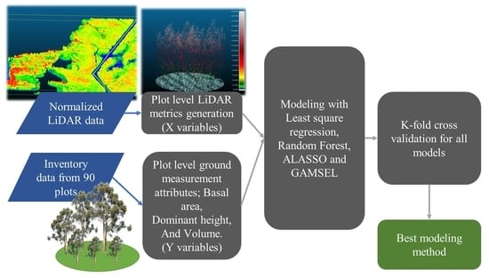
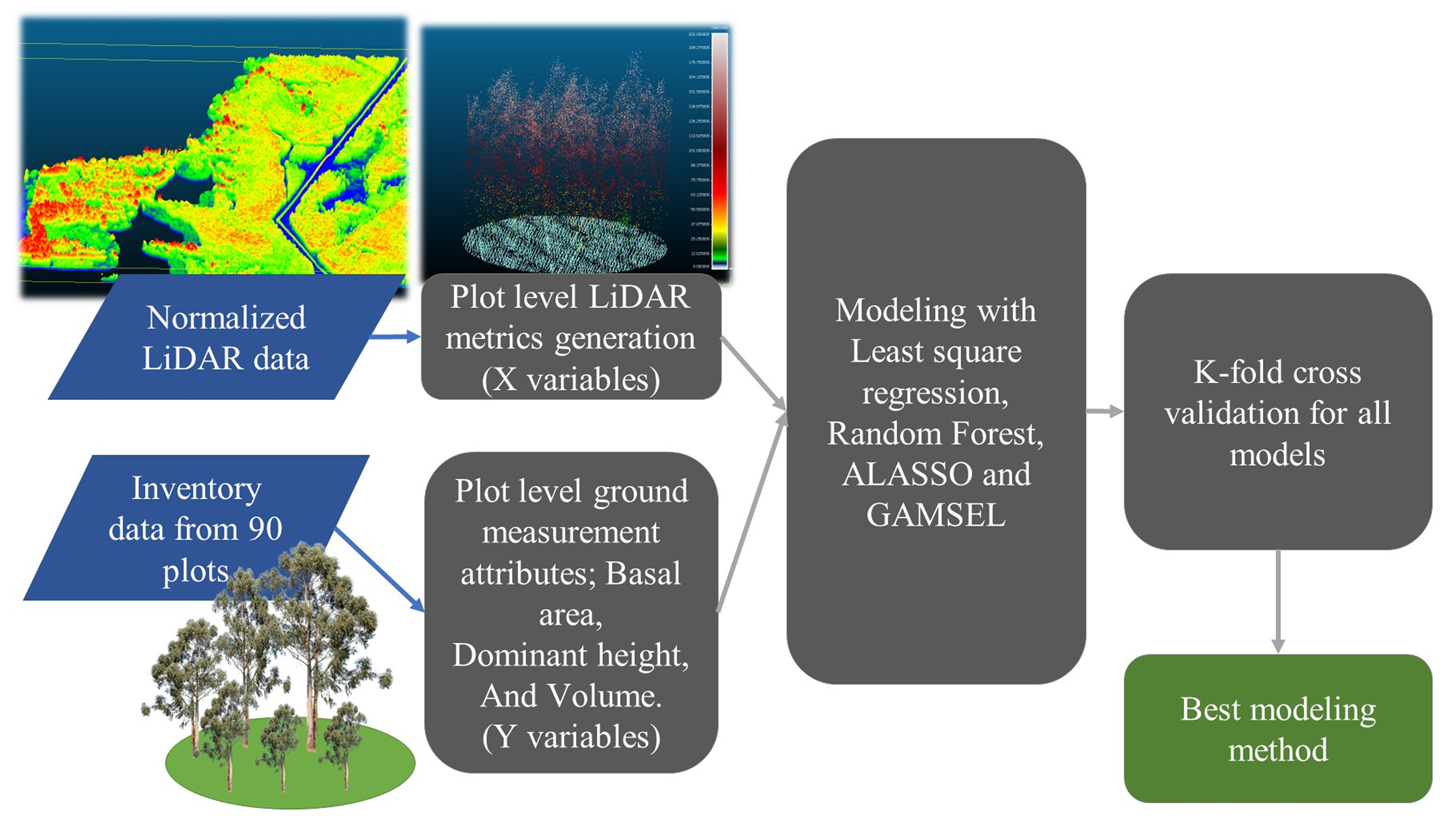
This research aims at developing equations to estimate forest attributes using two different modeling approaches—parametric and nonparametric regression for forest attribute prediction using lidar metrics. We evaluated four modeling methods: (1) Least squares regression (LSR), (2) adaptive least absolute shrinkage and selection operator (ALASSO), (3) random forest (RF), and (4) Generalized Additive Modeling Selection (GAMSEL). The last three methods aim to directly address the multicollinearity problem in ABA methodology while providing flexible model forms that might improve the relationship between lidar metrics and ground information.

2. Materials and Methods

2.1. Study Site

This study uses the data from an intensively managed Eucalyptus globulus plantation administrated by Manulife Investment Management in the Bio Bio region of central Chile (37°21′S; 73°20′W). Plantation ages range from 6 to 12 years. The area lies in a sub-humid and temperate climatic region with a maritime influence and four dry months per year. The temperature varies between 5.0 and 22.8 °C, with an average of 12.6 °C, and the mean annual rainfall is up to 1376 mm [52]. The predominant topography is hilly, with an elevation range of 80 m to 740 m. Soils in the plantation areas are deep marine sediments with loamy red clays on the surface and dark red clays in-depth, classified as Merilupo [53]. The soils are well structured, favoring deep root growth development and better soil water holding capacity. Figure 1 shows the study area and the distribution of inventory plots.

2.2. Field Data Collection

The field crew collected inventory data from April 12th to the 21st of 2021. Ninety circular plots of 400 m2 were established inside 69 lidar data acquisition square sites. The center of each circular plot was positioned using a global navigation satellite system. In each plot, the diameter of all trees greater than 15 cm at the breast height was measured using a diameter caliper, and the heights of ten dominating trees were measured with the Vertex. The latter information was used to develop a regression between height and diameter, to estimate all unmeasured heights from the plot using a linearized Schumacher type of Equation.
This study is focused on predicting three major variables needed for forest characterization: dominant height, basal area, and volume. Dominant height generally refers to the average height of the tallest trees in a forest. It is frequently used as a metric to assess a forest ecosystem’s general composition and vitality, with taller trees serving as an indicator of a more advanced and developed forest structure [54]. Similarly, the basal area measures the cumulative cross-sectional area of all tree stems at a given height, typically at breast height. It is a widely utilized variable in forestry and ecological management for characterizing the structural attributes of a forest stand. Likewise, tree volume is another important metric in forest ecology and management, which refers to the total volume of a tree stem, including the trunk and branches. It provides information on determining the wood quality, amount of biomass stored, harvest estimation, and various others that are essential for forest management and monitoring.
This study calculated the plot level dominant height as the average height from the 100 largest trees per hectare (the ones with the largest diameter) [54]. Basal area (BA) and volume were calculated by summing the individual tree data at the plot level and used as the response variable for this study. Equations of calculating the plot BA and volume are shown in Equations (1) and (2).
Basal area was calculated using Equation (1),
B A = i = 1 n ( ( π   × ( D B H i ) 2 4 × 10 , 000     )
where DBH is the breast height diameter (1.37 m from the ground) and 10,000 is a conversion factor that converts cm to square meters.
The merchantable volume per plot was calculated using the volume equation shown in Equation (2) up to a utilization index of 6 cm. Manulife Investment Management derived the equation from a sample of randomly selected eucalyptus trees between the ages of 5 and 12 years.
V o l u m e = β 0 × T P H β 1 × B A β 2 × H D o m β 3 × A g e β 4  
where T P H is the number of trees per hectare, B A is a basal area, H D o m is the dominant height of the plot, and Age is the Age of the stand. β0, β1, β2, β3, and β40 = 0.39239906, β1 = 0.04033281, β2 = 0.84491105, β3 = 0.85388192, and β4 = −0.18976973) are eucalyptus plantation specific parameters.

2.3. Lidar Data

This study used laser scanning data covering the study area collected by Manulife Investment Management group on 5 April 2021. The airborne laser scanner used was a discrete lidar sensor with a field of view of 40 degrees, and the flight altitude was 900 m. The average pulse density (the average number of pulses returned from the surface) was 43.6 points/m2 for the study area. Further specifications of the scanner are summarized in Table 1. For this study, we used 63 tiles distributed between the 37°32′12.32″S and 37°58′39.32″S latitude and between the 73°38′55.22″W and 73°06′23.08″W longitude.

2.4. Individual Tree Detection

While the primary focus of this study is to determine plot-level attributes, we also briefly examine the estimation of individual tree-level attributes, as it has been challenging in eucalyptus plantation forests in this region due to the intricate crown structure [55]. For individual tree detection, the first step of the data pre-processing, which involves noise filtering and normalization, was conducted by Manulife Investment Management Group. Then, we used the lidR package [56] in the R environment [57] for further processing. In order to identify individual trees using height-normalized lidar data, we first generated a 0.5 m resolution Canopy Height Model (CHM) using the ‘pitfree’ algorithm in the lidR package [58]. Subsequently, we utilized the CHM to apply a tree segmentation algorithm for individual tree detection, employing a local maxima-based algorithm [15]. Finally, we used a circular moving window with a fixed tree window size of 3 m × 3 m. Next, we applied this function to all sixty-three lidar tiles to calculate the number of trees in each plot for window sizes. The estimated number of trees was then added to the explanatory variable list for the tree density estimation.

2.5. Lidar Metrics Generation

Many studies have demonstrated that forest attributes such as the basal area, stand volume, and dominant height have a significant relationship with lidar height percentiles and density metrics [16,56,57]. Therefore, our explanatory variables in this study were lidar height percentiles and density metrics.
To generate the lidar height percentiles and density metrics listed in Table 2, we first clipped the normalized point cloud by the shape files defining the perimeter of the plots measured in the field. After that, 39 metrics were calculated at each plot level using elevation and pulse return values. A detailed description of those 39 metrics is presented in Table 2. Similarly, the summary statistics of all lidar metrics are described in Table 3.

2.6. Modeling Methods

In this study, we tested four modeling approaches (two parametric and two non-parametric) to predict ground-based variables. Two parametric methods are: The Ordinary Least Square (OLS), which provides us with a benchmark with respect to other common studies, and the adaptive least absolute shrinkage and selection operator (ALASSO), which is known to allow for a variable selection and to solve multicollinearity issues, at the expense of a small bias in the final prediction. Moreover, there are two non-parametric methods: The random forest regression (RF) and Generalized Additive Modeling Selection (GAMSEL). The former deals with collinearity by building decision trees with different sets of predictors and averaging them, and the later combines a series of basis functions with a penalization term (similar to ALASSO) to overcome multicollinearity. Each method was used to predict the basal area, dominant height, and merchantable volume using the lidar metrics described in Table 1. Details of each modeling approach are briefly introduced in the sections below:

2.6.1. Ordinary Least Squares Regression

Ordinary Least Squares (OLS) regression is a traditional data modeling approach, and is well-established for its simplicity and easy-making inferences with good predictive performances. The OLS fitting was performed using field-measured plot attributes as the response variable and lidar metrics as explanatory variables. To avoid a bias due to the multicollinearity between linear predictors, we used a subset regression approach to eliminate the high correlation between the explanatory variables to avoid a bias due to the multicollinearity between linear predictors. This approach identifies the subset of lidar-derived variables that best predicts the response variable using an efficient branch-and-bound algorithm implemented in the ‘leaps’ package in R to run the all-subset regression.
To identify the best models from the all-subset regression, we considered using the adjusted R-square (adj. R2), Mallow’s CP (CP), and Bayesian Information Criterion (BIC) because of their capability to address the overfitting issue. Model selection statistics such as the coefficient of determination (R2), which in modeling is the measure for goodness-of-fit based on the proportion of explained variance, becomes higher, and the residual sum of squares (RSS) becomes smaller when the model variables increase [58]. Thus, the model, including all variables, always results in the best selection statistics. The adjusted R2 deals with this problem by adjusting the value of R2 by considering the impact of additional independent variables in the model. Similarly, C p statistics address the limitation of R2 by adding a penalty to the training RSS to adjust the number of predictors in the model [59]. For a least square model with a fixed number of predictors, the C p is computed using Equation (3).
C p = 1 n ( RSS + 2 d σ ^ 2 )
where σ ^ 2 represents the estimated variance, n is the number of observations, d is the number of predictors, and the term 2 d σ ^ 2 is a penalty term that increases as the number of predictors in the model increases. Likewise, BIC is derived from a Bayesian point of view, and similar to C p , we selected the model with the lowest BIC value. For a least squares model containing d predictors, the BIC is computed using Equation (4).
BIC = 1 σ ^ 2 ( RSS + log ( n ) d σ ^ 2   )
Despite this method, variables selected by all subset regressions can also have a high correlation. Therefore, once several “best” models were identified based on adj R2, CP, and BIC, the variance inflation factor (VIF) and conditional indices (CI) were used to examine whether the variables were highly correlated. In a model, VIF and CI reflect the magnitude of the correlations between the independent variables. Thus, the larger values for these indices indicate a higher multicollinearity. According to Belsley, Kuh, and Welsch (1980), condition indices around 10 suggest weak correlations, while between 30 and 100 indicate moderate to strong correlations. If the condition index exceeds 100, it signifies serious multicollinearity issues [60]. Likewise, a VIF of above ten indicates the occurrence of multicollinearity among the predictor variables [44,61,62]. Hence, in this study, models that included explanatory variables with a VIF > 10 and CI > 30 were discarded from the final model.

2.6.2. Adaptive Least Absolute Shrinkage and Selection Operator Regression

The least absolute shrinkage and selection operator (LASSO) is a method of regression that has been gaining popularity in recent years, specifically in the statistical and machine learning field, due to its ability to handle high dimensional data sets [63]. This type of regression adds a penalization term to the loss function that shrinks the regression coefficients toward zero [49]. This is conducted by forcing the sum of the absolute value of the regression coefficients to be less than a fixed value (λ). After shrinkage, variables with a regression coefficient of zero are excluded from the model and, thus, constrain the complexity of the model [64].
Penalized regression methods attempt to achieve two fundamental goals of regression, predicting accurately and selecting the relevant variables simultaneously [65]. The major advantage of LASSO over conventional variable selection methods is that it performs a continuous variable selection and is more computationally feasible for larger datasets such as the variables used in this study. The lasso regression loss function can be defined as follows:
Y = β 0 + λ 1 × β 1 × x 1 + λ 2 × β 2 × x 2 λ n × β n × x n
where Y are dependent variables, and in our case, ground measured values for dominant height, basal area, and volume. Similarly, x 1 , x 2 , … x n are the independent variable, which in our case will be lidar metrics, β 0 ,   β 1 , β 2 β n are the regression coefficient for the independent variables. λ is the lasso shrinkage parameter that can shrink coefficients to zero.
This method needs a grid search method to find the best regularization parameters. Moreover, no proper regularization parameter allows this method to exploit the oracle properties defined by Fan and Li [66]. In the linear regression, an estimator that identifies the correct subset of actual variables and has an optimal estimation rate is known as the oracle properties. Thus, the adaptive lasso, which has oracle properties, was proposed as an alternative to improve the variable selection properties of the lasso [67]. It has the same advantages as the lasso; additionally, it avoids overfitting and penalizing large coefficients.
In linear regression, the lasso seeks to minimize:
Residual sum of square + λ   × (sum of the absolute value of the magnitude of coefficients)
i = 1 n ( y i β 0 j = 1 p β j x i j ) 2 +   λ   j = 1 p | β j |   = R S S +   λ   j = 1 p | β j |
where λ indicates the shrinkage amount and is chosen through a 10-fold cross-validation, β j is the estimated coefficients. When λ = 0, it implies that all features are included and, thus, equivalent to the linear regression.
Likewise, the adaptive lasso seeks to minimize the following:
R S S + λ j = 1 p w ^ j | β j |
where w ^ j is an adaptive weights vector parameter in the Equation. This weight vector performs different regularizations for each coefficient.
We used the k-fold cross-validation approach for this study to choose the best λ value. For this approach, we first randomly divided the dataset into ten sub-samples of equal size. After that, nine sub-samples were used to develop a prediction, and the remaining sub-sample validated the model. This procedure was performed ten times, with each of the ten sub-samples being used for validation and the others for model development. The result is produced by combining the ten different validation results for a range of λ values and choosing the preferred λ, which is then used to determine the final model. We used the “glmnet” package in R to perform the adaptive lasso regression for this study.

2.6.3. Random Forest

The RF algorithm is a nonparametric ensemble learning method for classification or regression based on several decision trees, which was developed by Breiman (2001). This method has several advantages with respect to the linear regression when the best lidar metrics selections are the ultimate goal: e.g., (1) Variable deletion is not required since it can handle a large number of input variables; (2) it estimates the variables that are important in the classification, measured as the mean decrease accuracy; (3) the generated forests can be saved for future use on other data; and (4) it reduces overfitting and is, therefore, more accurate compared to the boosted regression-based methods that are trained on the same data [68]. The regression was carried out using the ‘random forest’ [69] package in R. The accuracy of the RF-based method also depends on tuning parameters, such as ‘Ntree’ (i.e., number of trees grown) and ‘mtry’ (i.e., number of predictors sampled for splitting at each node); thus, their values have to be optimized carefully. Parameter values with complex rules tend to overfit the training data; as a result, a model performs very well for the training data but may yield the worst prediction for the independent data [70]. In the case of RF, the Out-of-Bag (OOB) observation method is widely used for selecting suboptimal parameter values to avoid the model overfitting. For this study, we used the ‘tuneRF’ function in random forest packages, which search for an optimal value for the parameters based on the OOB error estimation method.

2.6.4. Generalized Additive Modeling Selection (GAMSEL)

GAM (Generalized Additive Model) is a nonparametric extension of linear regression models which splits the regression lines into multiple segments and then applies local smoothing functions to track the non-linearity in the relationships between the dependent and independent variables [71]. In this study, we used an extension of GAMs called the Generalized Additive Modeling Selection (GAMSEL), a penalized likelihood method for fitting sparse generalized additive models, specifically for data with high dimensions. By allowing the effect of each variable to be estimated as either a linear, low-complexity curve or a zero as determined by the data, this method interpolates between null, linear, and additive models [50]. We used the ‘gamsel’ package in the R [72], where we first fitted the GAM model with all independent variables. After that, similarly to the ALASSO model, we applied a k-fold cross-validation with ten folds to find the best value for the penalization term, which is then used to fit the final model.

2.7. Model Validation

The k- fold cross-validation method was used to assess the accuracy of the four modeling approaches evaluated in this study. This approach involves a random division of the observations set into k groups, or folds, of equal size. Then, the first fold was used as a validation set, and the model was fitted on the remaining k-1 folds [59].
To do this, we first divided the datasets into nine folds (9 plots in one-fold). Then, the first fold was used as a validation set, and the model was fitted on the remaining eight folds. This procedure was repeated nine times with different subsets for validation. Finally, the model was used to predict the data on the first fold. An illustration of the k-fold cross-validation is shown in Figure 2.

3. Results

3.1. Summary Statistics and Variable Relationship

In the field-measured 90 plots, the highest plot dominant height measured was 35.23 m, and the lowest was 12.63 m. Likewise, the timber volume varied between 26 m3/ha to 363 m3/ha and BA between 6.21 m2/ha and 36.79 m2/ha. A more detailed statistical summary of field-measured attributes is shown in Table 4.
Figure 3 shows Pearson’s correlation coefficients between each response variable and the highly correlated four corresponding lidar metrics. This shows that the 75th and 80th percentiles, representing the middle and upper canopy of a stand, strongly correlate with the BA and the volume. Furthermore, the 90th and 95th percentiles had the highest correlation coefficient of 0.93 with the dominant height. Besides these four variables shown in Figure 3, all other response variables also demonstrate moderate to high correlations with the response variables.

3.2. Least Squares Regression Model

After the iterative variable selection process using the least squares regression, the final model retained only two predictors that satisfied the multicollinearity test, i.e., VIF and CI. In the final model for the volume and basal area, the 75th percentile of the echo height and the percentage of the first return above the mean echo height were the two variables retained (Equations (8) and (9)). For both equations, the 75th percentile had the most significant coefficient, indicating its higher relative importance for predicting both the volume and basal area.
Volume = 5.271 + 0.5176 p 75 + 0.0612 rp 1
BA = 0.414 + 0.0486 p 75 + 0.0103 rp 1
where p 75 is the 75th percentile of echo height, and r p 1 is the percentage of the first returns above the mean.
Likewise, for the dominant height, as shown in Equation (10), the 90th and 40th percentiles of the echo height are the two variables that are held in the model while keeping the collinearity indices within the acceptable range. Details of VIF and CI values for each selected variable are presented in Table 5.
Dom .   height = 1.466 + 1.196 p 90 + 0.132 p 10
where p 90 is the 90th percentile of the echo height, and x2 is the 40th percentile of the echo height.

3.3. Random Forest

In RF-based models, height percentile variables were the most important for all three response variables. As shown in Figure 4, the 90th, 75th, and 80th percentiles of the echo height were the most significant variables for estimating the volume. Similarly, all echo height metrics that describe the upper canopy level, namely the 95th, 80th, 90th, and 99th percentiles, were the most important variables for the dominant height estimation model. Finally, in the basal area model, the mid-canopy echo heights, i.e., the 60th and 65th percentiles of height, and the variable “percentage of first return above mean” are the most important metrics. A summary of all important variables is shown in Figure 4.

3.4. ALASSO Regression Model

The ALASSO method retained nine, eight, and eight variables on the final model for volume, basal area, and dominant height, respectively. The 1st percentile of the echo height and the first return ratio over the mean appeared in all three models; likewise, the 75th percentile, 85th percentile of echo height, and percentage of the first return above minimum height, as well as above the mean, were other selected variables in the model. For volume prediction, the 1st percentile of the echo height was the most significant variable, with a coefficient of 1.122, followed by the 80th percentile height, with a coefficient of 0.25. The canopy relief ratio was the most crucial variable in the basal area model, followed by the 1st percentile of the echo height with a coefficient of 0.549 and 0.08, respectively. Likewise, the 1st percentile of the echo height with a coefficient of 0.69 has the highest impact, followed by the 90th percentile with a coefficient of 0.58 on the dominant height model. A list of all the variables and their coefficients selected for volume, BA, and the dominant height model with ALASSO is shown in Table 6.

3.5. Generalized Additive Modeling Selection

Using the GAMSEL method, we obtained eleven variables for the basal area (BA) model, nine for the volume model, and five for the dominant height model. A common variable in all three models was the ‘first return percentage above the mean’, which reflects the canopy cover and structure in the stand. It was also one of the highly significant variables for the volume and basal area, as shown in Figure 5 and Figure 6. In a similar manner, the basal area and volume, height means, height kurtosis, first percentile, 25th percentile, 80th percentile, and all returns above the mean and first return ratio were the repeating variables. Moreover, for volume, besides the first return percentage above the mean, the 80th and 25th percentile were the other key variables in the model representing the upper and lower canopy, respectively. Likewise, for the basal area and echo height means, all return percentages above the mean and 75th percentile were the key variables in addition to the first return percentage above the mean, 80th, and 25th percentile.
As described earlier, one significant benefit of the GAM model is that it can incorporate a non-linear relationship between the response and predictor variable. Hence, in our final GAMSEL model, all variables retained had a non-linear relationship with respect to the response variable. The detailed relation between all selected variables (with nonzero coefficients) for basal area, volume, and dominant height models with the function of the last lambda value is shown in Figure 5, Figure 6 and Figure 7, respectively.

3.6. Model Comparison Summary

In this comparison, for volume, the highest R2 of 0.88 was achieved with ALASSO and GAMSEL, and ALASSO yielded the lowest RMSE of 0.781 m3/plot. Likewise, the highest R2 of 0.83 and the lowest RMSE of 0.109 for the basal area were achieved with the ALASSO method. In the dominant height case, ALASSO and GAMSEL yielded the highest R2 of 0.87. The least RMSE of 1.353 m was achieved using the least squares modeling method. Consistent with the RMSE, the lowest Mean Square Error (MSE) was attained for the volume and basal area models using the ALASSO method, followed by the GAMSEL method. For the dominant height model, the minimum MSE was achieved using the least squares (LS) method, followed by the ALASSO method. Table 7 summarizes the k-fold cross-validation results for four modeling methods. Figure 8 shows the residual vs. fitted plot for the volume, BA, and dominant height for the ALASSO model. Overall, the ALASSO method demonstrated a better consistency and produced residual plots with fewer biases compared to the other three methods. A detailed residual vs. fitted plot for the volume, BA, and dominant height for all four modeling methods is shown in Appendix A.

3.7. Individual Tree Detection

The individual tree detection method performed very poorly, yielding a correlation of 0.018 when comparing the number of trees detected by the model with the tree density measured in the field. However, when combining the number of trees estimated with the segmentation algorithm with the other thirty-nine metrics and applying the least squares regression, the model accuracy (adjusted R2) increased to 0.15. Likewise, for model accuracy, the random forest and GAMSEL regression methods achieved 0.18 and 0.178, respectively. Additionally, when incorporating all 39 lidar metrics and the number of trees estimated by the algorithm for each plot as explanatory variables in the ALASSO regression method, we obtained a comparable adjusted R-squared value of 0.18 to that of the other methods.

4. Discussion

In recent decades, several forest-related industries around the globe have adopted laser scanning as auxiliary information to complement forest inventories. However, the modeling methods in use for the forest parameter estimation are still not adequately exploiting the information in the point clouds [
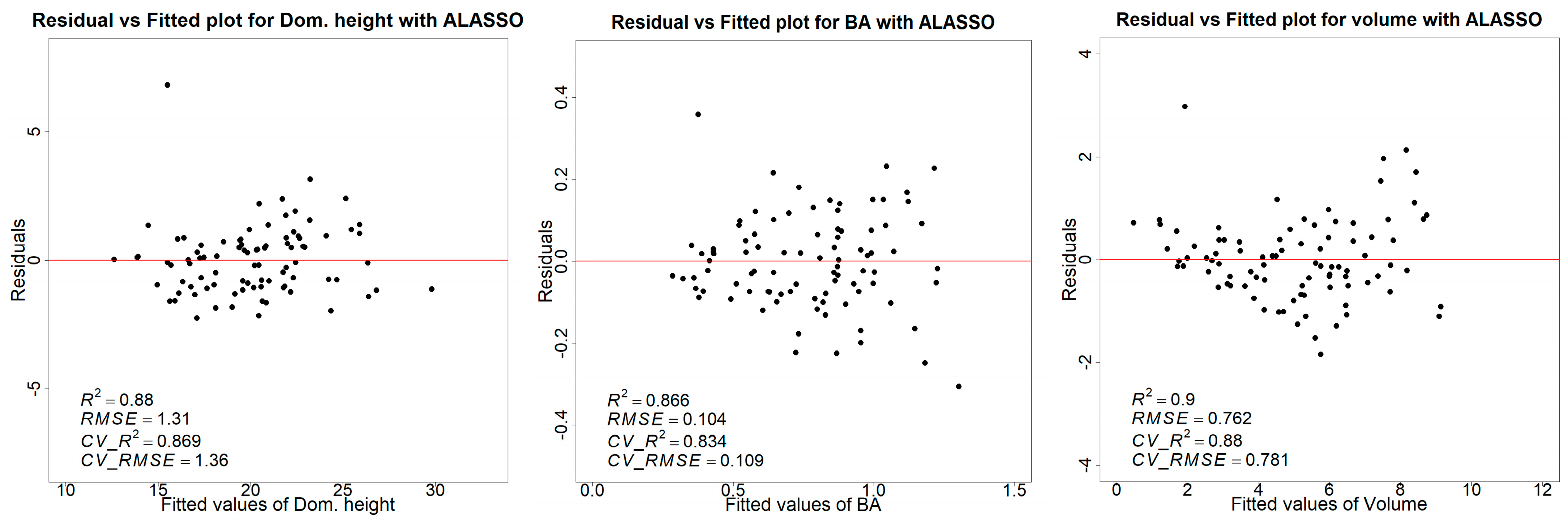
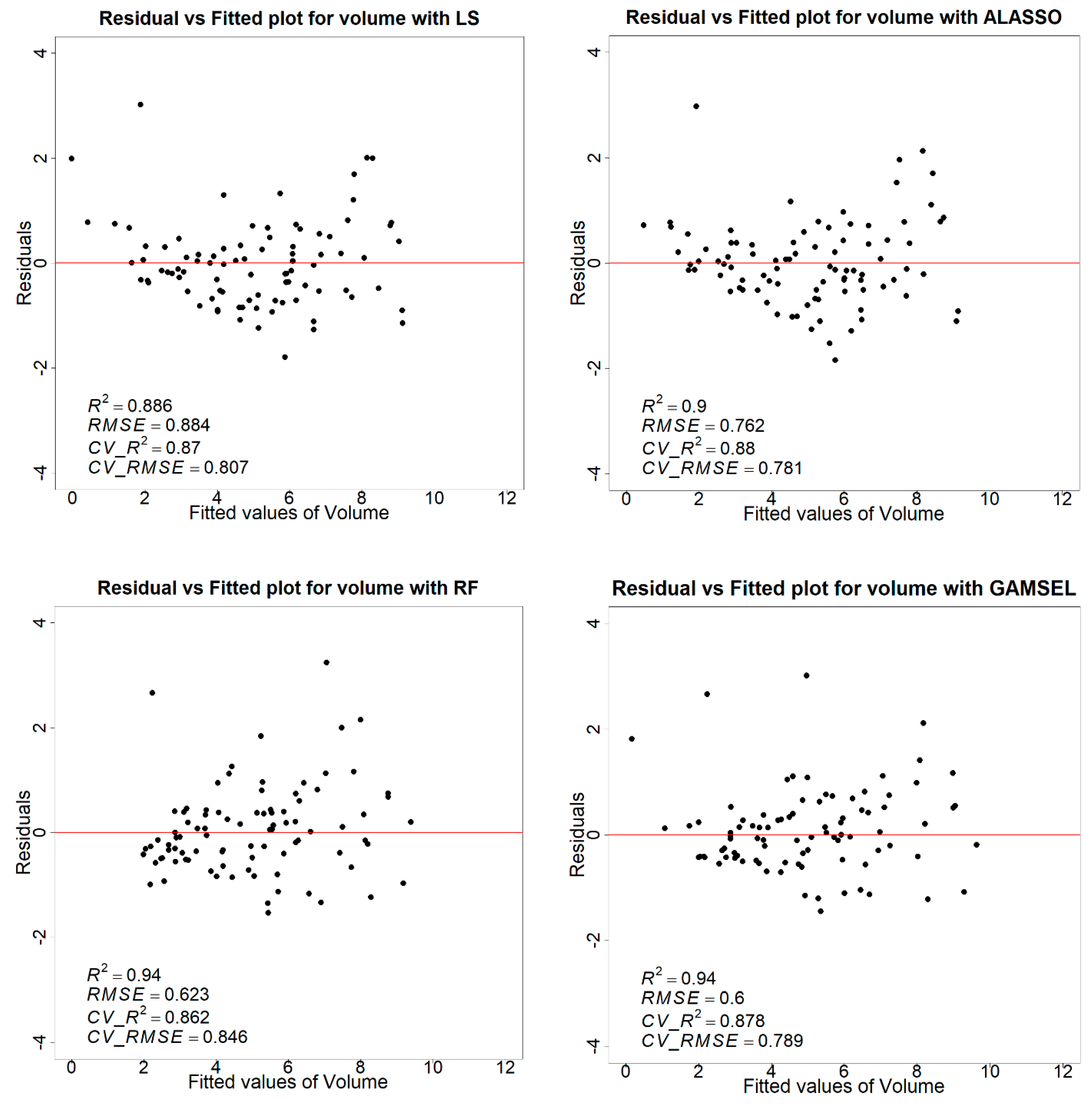
73]. In this study, we compared the performance of four different modeling methods to predict various forest attributes using aerial lidar data. When comparing those four methods for volume estimation, adaptive lasso performed better than the other three. Although the overall coefficient of determination (adj. R2) of 0.88 and the lowest RMSE of 19.53 m3/ha was achieved in this study with adaptive lasso regression, the difference compared to other methods is very nominal, i.e., 19.73 m3/ha, 20.18 m3/ha, and 21.15 m3/ha with respect to the GAMSEL, LS (least squares), and random forest, respectively. The RMSE of 19.53 m3/ha is low compared to other studies in similar forest conditions. A possible reason for this might be lidar data with better point cloud density (44 points/m2) and a relatively smaller study area than other studies. Leite et al. (2020) compared a few parametric and nonparametric regression methods for the area-based volume estimation of a eucalyptus plantation using low-lidar data (5 points/m2) and concluded the best result of adj. R2 0.83 and RMSE 40.71 m3/ha using the artificial neural network (ANN) and the lowest of adj. R2 0.79 and RMSE 46.76 m3/ha with the linear regression method [74]. Likewise, Silva et al. (2016) applied the principal component approach for predicting the stem volume in eucalyptus plantations using a lidar metric generated from medium-density (10/points/m2) lidar point clouds. They achieved an adj R2 of 0.87 and RMSE of 27.60 m3/ha [56].
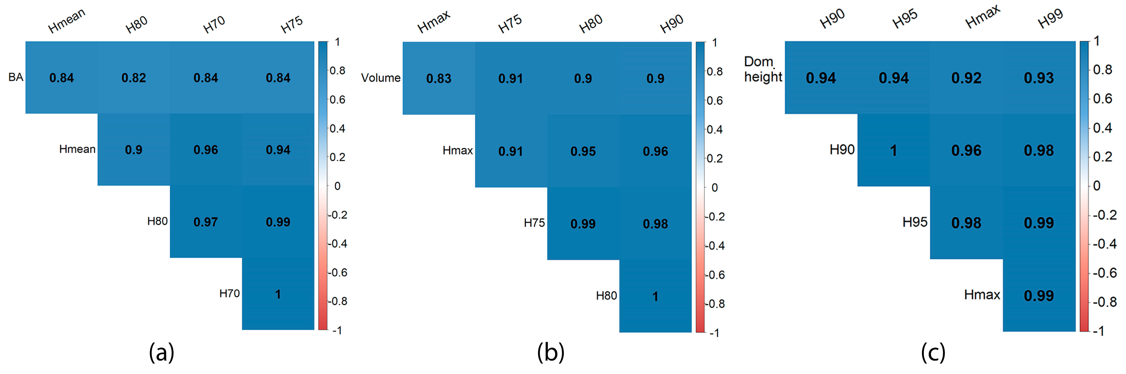
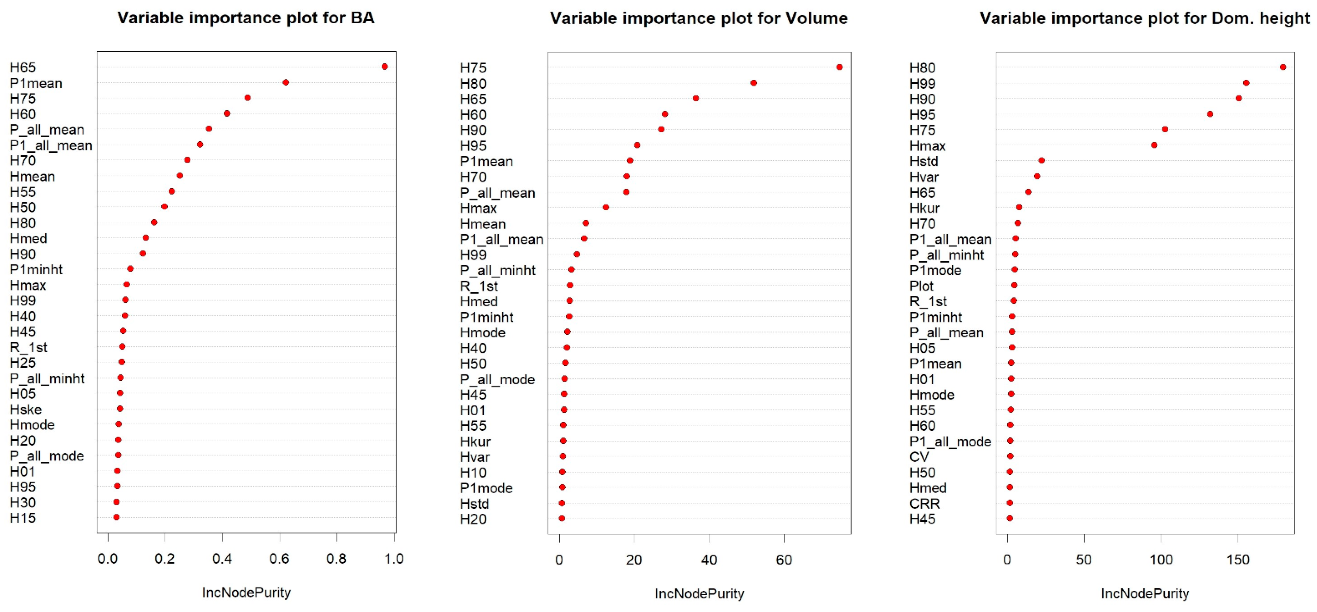
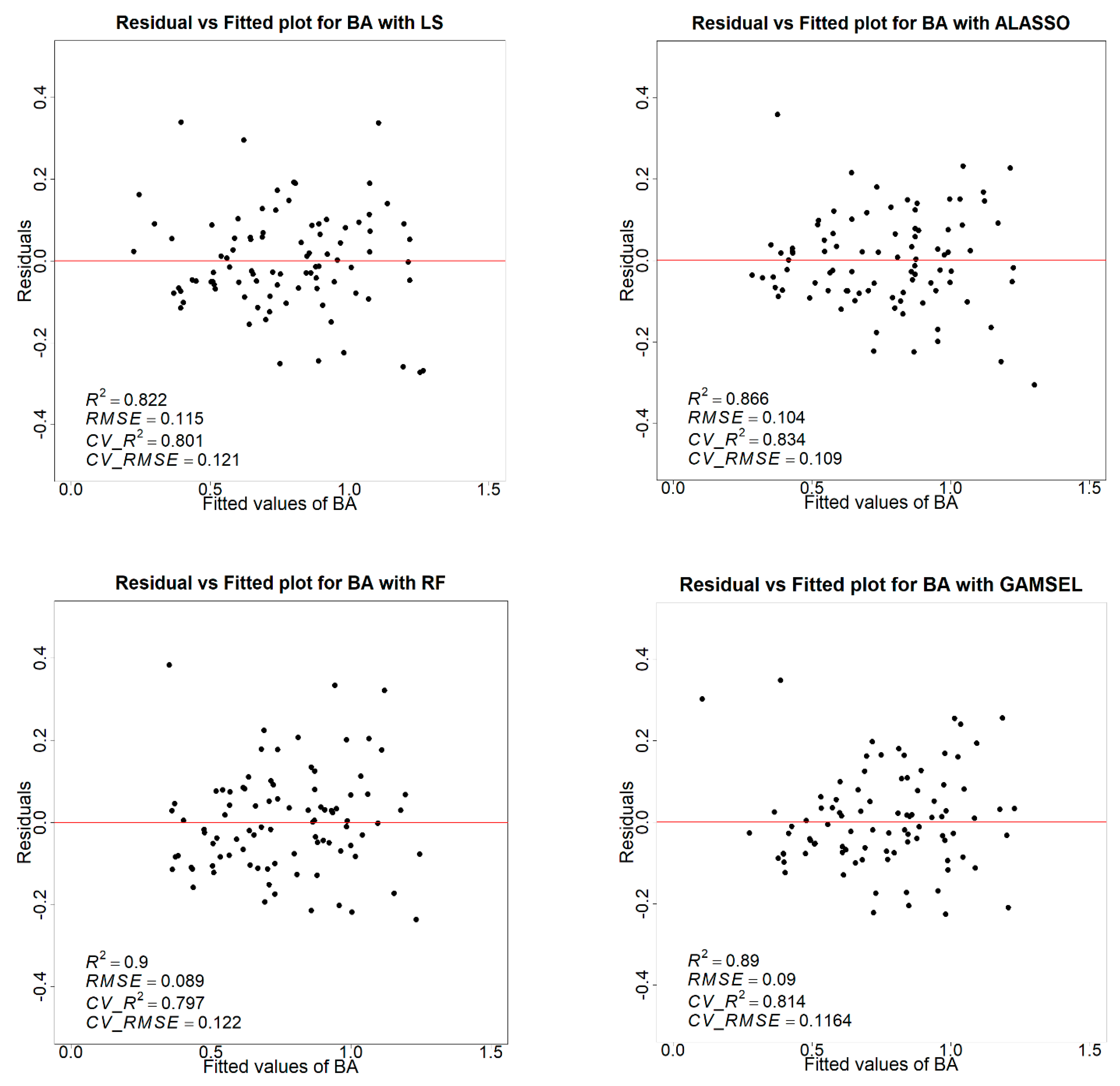
In this study, the 75th percentile of height was included in all four models as a vital metric for estimating the volume. After the 75th percentile, the 90th percentile, canopy relief ratio, and percentage of the first return above the mean are primary metrics predicting the volume. Consistent with the outcome obtained for the volume model, the optimal model for the basal area was determined using the adaptive lasso regression method. The adaptive lasso regression slightly improved the prediction for the basal area with an overall adj. R2 of 0.83 and RMSE 2.73 m2/ha compared to the adj. R2 of 0.81, 0.80, and 0.80 and RMSE of 2.90 m2/ha, 3.03 m2/ha, and 3.05 m2/ha with GAMSEL, LS, and random forest, respectively. Likewise, for the dominant height, both the adaptive lasso and GAMSEL model achieved the highest adj. R2 of 0.87 followed by LS and random forest regression methods with an adj. R2 of 0.86 and 0.83, respectively. However, in terms of better RMSE for dominant height, the least square method resulted in a slightly better RMSE of 33.83 m/ha, followed by the adaptive lasso, GAMSEL, and the random forest with an RMSE of 33.98 m/ha, 33.53 m/ha, and 38.82 m/ha, respectively. Other researchers, such as Brown et al. (2022), compared linear and random forest methods for the basal area estimation using variables from the low-density lidar and multispectral imageries. In that study, they achieved a slightly better result with the random forest method (R2 of 0.39 and 0.36, and RMSE of 5.662 m2/ha and 5.731 m2/ha with the random forest and LS, respectively) but an overall low accuracy compared to our study [57]. In another study by Li et al. (2022), they proposed a model with a good generalization capability for the basal area using lidar-derived metrics for eucalyptus plantation forests achieving an R2 of 0.71 and rRMSE of 18.22% [75] using the least square method.
Furthermore, Li et al. (2022) used an exhaustive combination of lidar metrics with a clear meaning in forest mensuration. They formulated 86 tree type-specific and region-generalized models and sorted the most meaningful variables for estimating the stand volume and basal area. In that study, they found the 75th and 95th percentile, the percentage of the first returns above the minimum height, and the standard height deviation as important variables for the basal area estimation. Similarly to this is the 95th percentile, first return ratio above the mean height, and the coefficient of a height variance for the volume estimation in the eucalyptus forest [75]. The 50th to 75th percentile represents the middle and upper part of the stand canopy; likewise, the 80th to 99th percentile characterizes the upper part of the canopy [29,
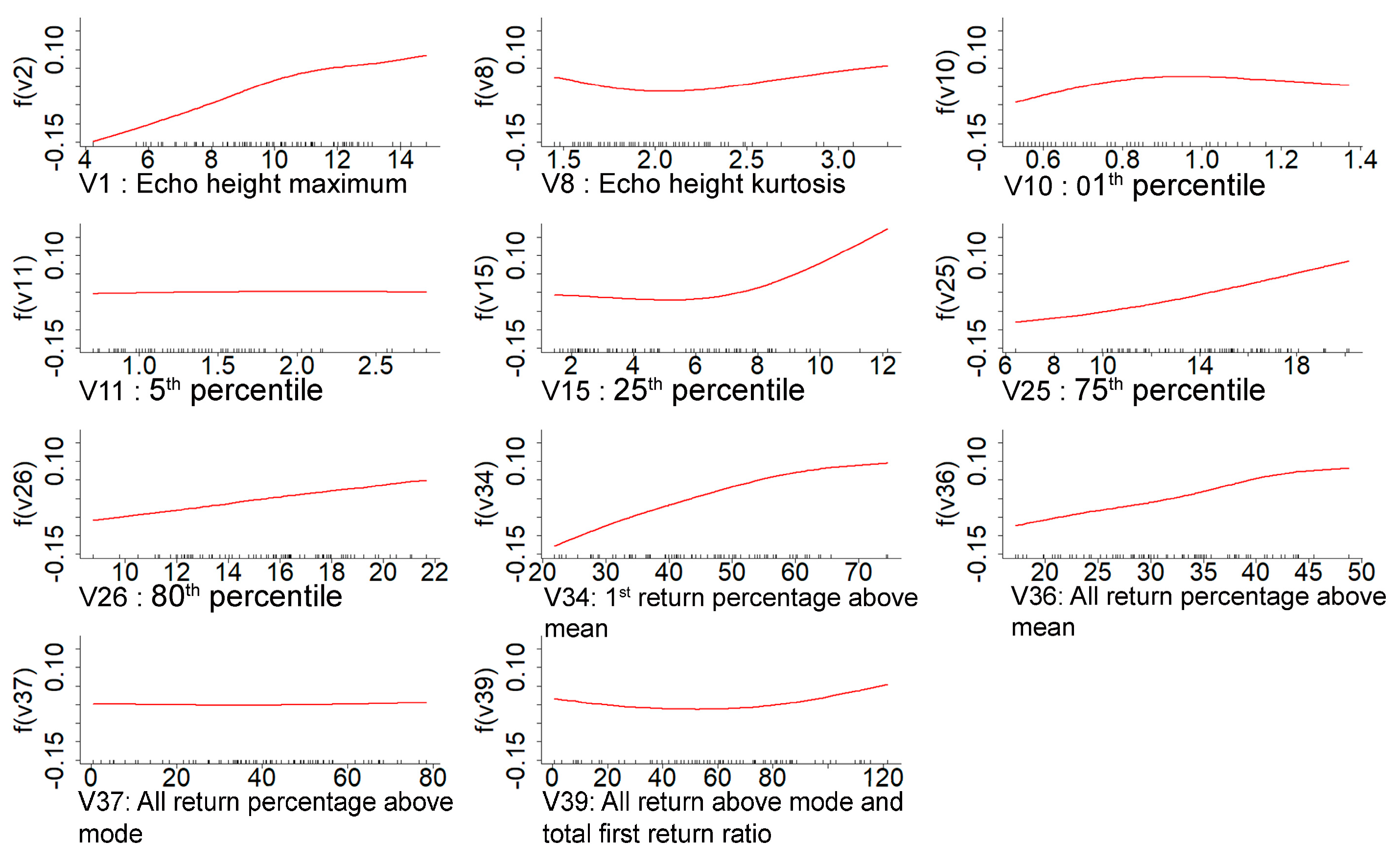
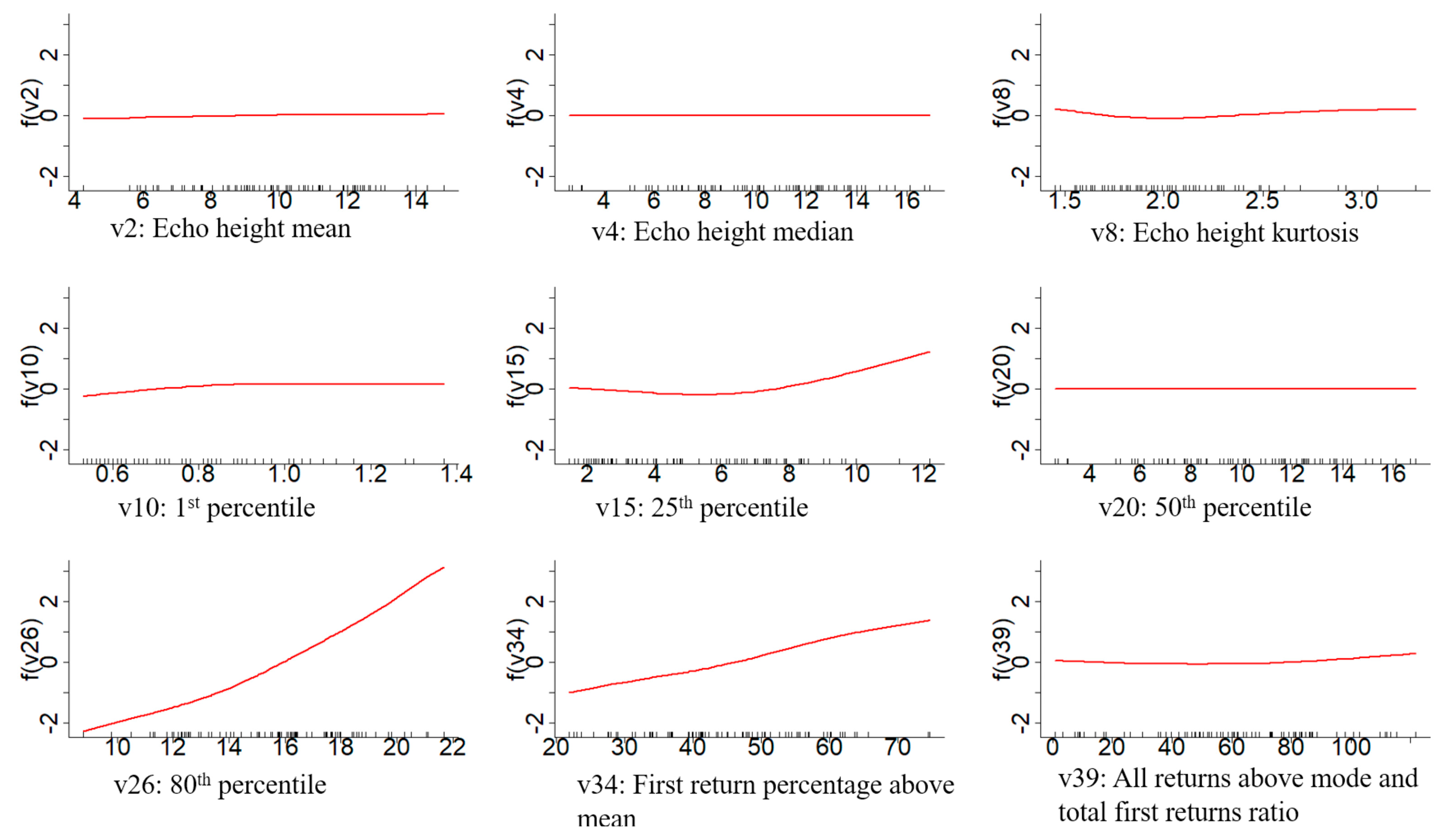
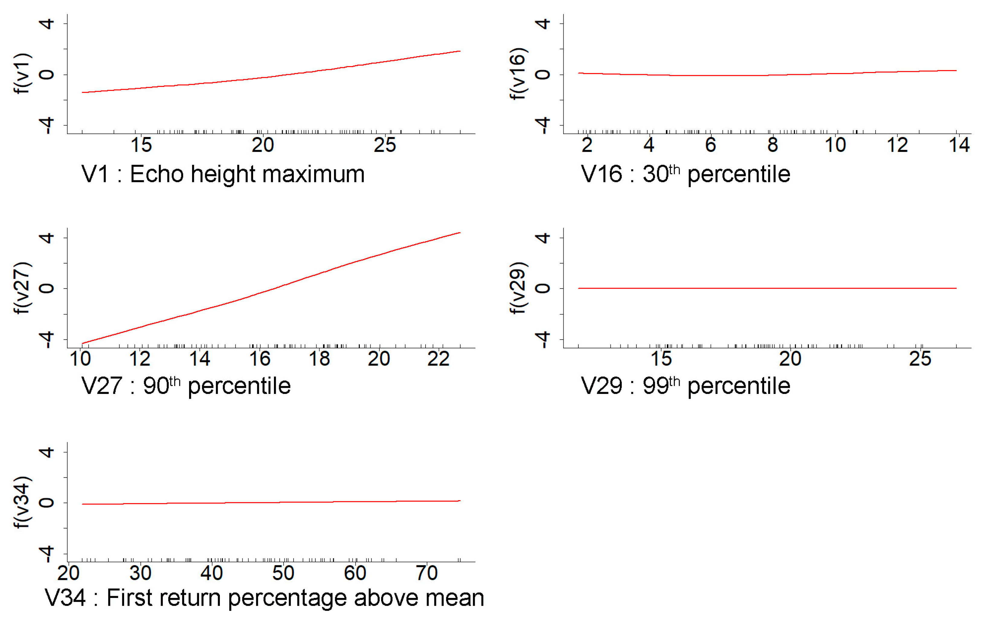
76]. Therefore, including these mid and upper-canopy percentiles and density metrics representing the crown structure and cover makes the model more generalizable and significant. This result corresponds with the variables selected in our models. In our study, the 75th percentile of the echo height and the percentage of the first returns above the mean are the two significant variables in the LS model for the basal area and volume. Comparably, the foremost contributing variables in the random forest model are the height percentiles representing the canopy’s middle and upper parts, and the minimal contributing variables are below the 40th percentile. Corresponding to the LS and random forest, the most significant variables in the GAMSEL model are also from the middle and upper percentiles and density ratio variables representing the canopy structure and cover. However, the variables included in the adaptive lasso are distinct from the other three since the most contributing variable for the basal area is the canopy relief ratio, and for volume and dominant height, it is the first percentile of echo height. Although these selected variables are not among the topmost variables in the other three models, they have similar properties to those selected variables in the other three models. The canopy relief ratio is the ratio of the mean and maximum value of all echo heights in a given area, signifying the canopy structure like other density metrics. Similarly, the first percentile represents the bottom portion of the stem and tends to fluctuate evenly according to the stem density.
We tested the performance of popular parametric, semiparametric, and nonparametric modeling methods for the forest attribute estimation. In our test, the semiparametric models, i.e., the adaptive lasso and GAMSEL, slightly improved the estimates; however, none performed significantly differently from the others. Kangas et al. (2016), in their study of the aboveground biomass (AGB) estimation, tested the parametric, semiparametric, and nonparametric models using real-world and simulated lidar-based variables. In that comparison, although they achieved a better accuracy with the nonparametric model, i.e., local constant kernel, they found it leading to the underestimation of the variance; thus, they recommended using the semiparametric, i.e., GAM, which they found more consistent and suitable for the internal model [77]. On the other hand, even though parametric models such as the least squares regression are a more straightforward method, applications at a practical scale are scarcer. One primary reason is that when the number of dependent variables is very high, evaluating each variable to obtain a meaningful model conforming to all assumptions is not practical [78]. Hence, even though our results demonstrate the nominal difference in accuracies between the evaluated models, the semiparametric model seems more fitting to apply in a practical scenario.
In our study, the individual tree detection method failed to estimate the total number of trees in the plot correctly. One probable reason for such low correlations can be the small sample plot size of just 400 m2, resulting in the insufficient number of trees to adjust the error due to the trees in the plot boundary. Moreover, in the field inventory, a standard GNSS receiver was used to establish the plot center, which might also have contributed to the low accuracy of ITD. Some studies have suggested that using a higher-density lidar point cloud will improve the ITD accuracy. However, a study was conducted in a similar eucalyptus plantation forest by Corte et al. (2022), and applying a similar ITD approach in high-density lidar data (>1400 pts/m2) did not noticeably contribute to improving the accuracy (average R2 = 0.24). They mentioned a complex stand structure and irregular branching forms of the eucalyptus causing omission and commission when outlining trees, in addition to the error associated with the GPS positioning as the major limitation [55]. Those mentioned limitations are also the case in our study. In addition, half of the sample plots are from regrowth forests with complex branching and multiple stems; it was challenging to delineate the crown of every branch.

5. Conclusions

In our study, the assessment of various methods for forest attribute estimation using high-dimensional lidar metrics showed no method to be superior to the others in terms of significant advantage. The ALASSO method, however, demonstrated the highest R2 values of 0.88, 0.83, and 0.87 for the volume, basal area, and dominant height, respectively. Furthermore, GAMSEL and LSR followed this method regarding the performance and lack of bias.
In conclusion, this study provides insights into the performance of different modeling methods for predicting forest attributes using aerial lidar data. In light of this result and the ease of implementation, we recommend using the ALASSO method for the forest attribute estimation. However, further research is needed to investigate the generalizability of these results to other forest types and conditions.

Author Contributions

Conceptualization, C.R.M.; methodology, C.R.M. and A.P.; software, A.A.; validation, C.R.M. and A.P.; formal analysis, A.A.; writing—original draft preparation, A.A.; writing—review and editing, C.R.M. and A.P.; supervision, A.P.; funding acquisition, C.R.M. and A.P. All authors have read and agreed to the published version of the manuscript.

Funding

The Warnell School of Forestry and Natural Resources at the University of Georgia provided funding support for the author’s graduate assistantship and the Plantation Management Research Cooperative for publication efforts.

Data Availability Statement

The data provided for this research is not publicly available.

Acknowledgments

The authors would like to thank Manulife Investment Management for providing the data for this research, both lidar data acquisition and plot forest inventory data.

Conflicts of Interest

The authors declare no conflict of interest.

Appendix A

Figure A1. Each panel shows the residual vs. fitted plot for volume with LS, ALASSO, RF, and GAMSEL models. R2 and RMSE are the model accuracy before cross-validation, and CV_R2 and CV RMSE show the model accuracy result of nine-fold cross-validation.
Remotesensing 15 01284 g0a1
Figure A2. Each panel shows the residual vs. fitted plot for the basal area with LS, ALASSO, RF, and GAMSEL models. R2 and RMSE are the model accuracy before cross-validation, and CV_R2 and CV RMSE show the model accuracy result of nine-fold cross-validation.
Remotesensing 15 01284 g0a2
Figure A3. Each panel shows the residual vs. fitted plot for dominant height with LS, ALASSO, RF, and GAMSEL models. R2 and RMSE are the model accuracy before cross−validation, and CV_R2 and CV_RMSE show the model accuracy result of nine−fold cross−validation.
Remotesensing 15 01284 g0a3

References

  1. Lovell, J.L.; Jupp, D.L.B.; Newnham, G.J.; Coops, N.C.; Culvenor, D.S. Simulation study for finding optimal lidar acquisition parameters for forest height retrieval. For. Ecol. Manag. 2005, 214, 398–412. [Google Scholar] [CrossRef]
  2. White, J.C.; Coops, N.C.; Wulder, M.A.; Vastaranta, M.; Hilker, T.; Tompalski, P. Remote sensing technologies for enhancing forest inventories: A review. Can. J. Remote Sens. 2016, 42, 619–641. [Google Scholar] [CrossRef] [Green Version]
  3. McRoberts, R.E.; Tomppo, E.O. Remote sensing support for national forest inventories. Remote sensing of environment 2007, 110, 412–419. [Google Scholar] [CrossRef]
  4. Liang, X.; Kankare, V.; Hyyppä, J.; Wang, Y.; Kukko, A.; Haggrén, H.; Yu, X.; Kaartinen, H.; Jaakkola, A.; Guan, F. Terrestrial laser scanning in forest inventories. ISPRS J. Photogramm. Remote Sens. 2016, 115, 63–77. [Google Scholar] [CrossRef]
  5. Brown, S. Estimating Biomass and Biomass Change of Tropical Forests: A Primer; Food & Agriculture Org.: Rome, Italy, 1997; Volume 134. [Google Scholar]
  6. Picard, N.; Saint-André, L.; Henry, M. Manual for building tree volume and biomass allometric equations: From field measurement to prediction. In Manual for Building Tree Volume and Biomass Allometric Equations: From Field Measurement to Prediction, FAO; Food and Agricultural Organization of the United Nations: Rome, Italy, 2012. [Google Scholar]
  7. Holopainen, M.; Kalliovirta, J. Modern data acquisition for forest inventories. In Forest Inventory; Springer: Berlin/Heidelberg, Germany, 2006; pp. 343–362. [Google Scholar]
  8. Pajeres, G. Overview and current status of remote sensing applications based on unmanned aerial vehicles. Photogramm. Eng. Remote Sens. 2015, 81, 281–329. [Google Scholar] [CrossRef] [Green Version]
  9. Toth, C.; Jóźków, G. Remote sensing platforms and sensors: A survey. ISPRS J. Photogramm. Remote Sens. 2016, 115, 22–36. [Google Scholar] [CrossRef]
  10. Zhu, L.; Suomalainen, J.; Liu, J.; Hyyppä, J.; Kaartinen, H.; Haggren, H. A review: Remote sensing sensors. Multi-Purp. Appl. Geospat. Data 2018, 71049, 19–42. [Google Scholar]
  11. Salas, C.; Ene, L.; Gregoire, T.G.; Næsset, E.; Gobakken, T. Modelling tree diameter from airborne laser scanning derived variables: A comparison of spatial statistical models. Remote Sens. Environ. 2010, 114, 1277–1285. [Google Scholar] [CrossRef]
  12. Ørka, H.O.; Jutras-Perreault, M.-C.; Candelas-Bielza, J.; Gobakken, T. Delineation of Geomorphological Woodland Key Habitats Using Airborne Laser Scanning. Remote Sens. 2022, 14, 1184. [Google Scholar] [CrossRef]
  13. Reutebuch, S.E.; Andersen, H.-E.; McGaughey, R.J. Light detection and ranging (LIDAR): An emerging tool for multiple resource inventory. J. For. 2005, 103, 286–292. [Google Scholar]
  14. Næsset, E.; Gobakken, T.; Holmgren, J.; Hyyppä, H.; Hyyppä, J.; Maltamo, M.; Nilsson, M.; Olsson, H.; Persson, Å.; Söderman, U. Laser scanning of forest resources: The Nordic experience. Scand. J. For. Res. 2004, 19, 482–499. [Google Scholar] [CrossRef]
  15. Popescu, S.C.; Wynne, R.H. Seeing the trees in the forest. Photogramm. Eng. Remote Sens. 2004, 70, 589–604. [Google Scholar] [CrossRef] [Green Version]
  16. Asner, G.P.; Mascaro, J.; Muller-Landau, H.C.; Vieilledent, G.; Vaudry, R.; Rasamoelina, M.; Hall, J.S.; Van Breugel, M. A universal airborne LiDAR approach for tropical forest carbon mapping. Oecologia 2012, 168, 1147–1160. [Google Scholar] [CrossRef] [PubMed]
  17. Ioki, K.; Tsuyuki, S.; Hirata, Y.; Phua, M.-H.; Wong, W.V.C.; Ling, Z.-Y.; Saito, H.; Takao, G. Estimating above-ground biomass of tropical rainforest of different degradation levels in Northern Borneo using airborne LiDAR. For. Ecol. Manag. 2014, 328, 335–341. [Google Scholar] [CrossRef]
  18. Coops, N.C.; Tompalski, P.; Goodbody, T.R.H.; Queinnec, M.; Luther, J.E.; Bolton, D.K.; White, J.C.; Wulder, M.A.; van Lier, O.R.; Hermosilla, T. Modelling lidar-derived estimates of forest attributes over space and time: A review of approaches and future trends. Remote Sens. Environ. 2021, 260, 112477. [Google Scholar] [CrossRef]
  19. Popescu, S.C.; Wynne, R.H.; Nelson, R.F. Measuring individual tree crown diameter with lidar and assessing its influence on estimating forest volume and biomass. Can. J. Remote Sens. 2003, 29, 564–577. [Google Scholar] [CrossRef]
  20. Li, W.; Guo, Q.; Jakubowski, M.K.; Kelly, M. A new method for segmenting individual trees from the lidar point cloud. Photogramm. Eng. Remote Sens. 2012, 78, 75–84. [Google Scholar] [CrossRef] [Green Version]
  21. Naesset, E. Determination of mean tree height of forest stands using airborne laser scanner data. ISPRS J. Photogramm. Remote Sens. 1997, 52, 49–56. [Google Scholar] [CrossRef]
  22. Næsset, E. Predicting forest stand characteristics with airborne scanning laser using a practical two-stage procedure and field data. Remote Sens. Environ. 2002, 80, 88–99. [Google Scholar] [CrossRef]
  23. Koch, B.; Heyder, U.; Weinacker, H. Detection of individual tree crowns in airborne lidar data. Photogramm. Eng. Remote Sens. 2006, 72, 357–363. [Google Scholar] [CrossRef] [Green Version]
  24. Silva, C.A.; Hudak, A.T.; Vierling, L.A.; Loudermilk, E.L.; O’Brien, J.J.; Hiers, J.K.; Jack, S.B.; Gonzalez-Benecke, C.; Lee, H.; Falkowski, M.J. Imputation of individual longleaf pine (Pinus palustris Mill.) tree attributes from field and LiDAR data. Can. J. Remote Sens. 2016, 42, 554–573. [Google Scholar] [CrossRef]
  25. Bian, Y.; Zou, P.; Shu, Y.; Yu, R. Individual tree delineation in deciduous forest areas with LiDAR point clouds. Can. J. Remote Sens. 2014, 40, 152–163. [Google Scholar] [CrossRef]
  26. Kwak, D.-A.; Lee, W.-K.; Lee, J.-H.; Biging, G.S.; Gong, P. Detection of individual trees and estimation of tree height using LiDAR data. J. For. Res. 2007, 12, 425–434. [Google Scholar] [CrossRef]
  27. Hirata, Y.; Furuya, N.; Suzuki, M.; Yamamoto, H. Airborne laser scanning in forest management: Individual tree identification and laser pulse penetration in a stand with different levels of thinning. For. Ecol. Manag. 2009, 258, 752–760. [Google Scholar] [CrossRef]
  28. Goerndt, M.E.; Monleon, V.J.; Temesgen, H. Relating forest attributes with area-and tree-based light detection and ranging metrics for western Oregon. West. J. Appl. For. 2010, 25, 105–111. [Google Scholar] [CrossRef] [Green Version]
  29. Bouvier, M.; Durrieu, S.; Fournier, R.A.; Renaud, J.-P. Generalizing predictive models of forest inventory attributes using an area-based approach with airborne LiDAR data. Remote Sens. Environ. 2015, 156, 322–334. [Google Scholar] [CrossRef]
  30. Gleason, C.J.; Im, J. A review of remote sensing of forest biomass and biofuel: Options for small-area applications. GIScience Remote Sens. 2011, 48, 141–170. [Google Scholar] [CrossRef]
  31. Hall, S.; Burke, I.; Box, D.; Kaufmann, M.; Stoker, J.M. Estimating stand structure using discrete-return lidar: An example from low density, fire prone ponderosa pine forests. For. Ecol. Manag. 2005, 208, 189–209. [Google Scholar] [CrossRef]
  32. Lim, K.; Treitz, P.; Baldwin, K.; Morrison, I.; Green, J. Lidar remote sensing of biophysical properties of tolerant northern hardwood forests. Can. J. Remote Sens. 2003, 29, 658–678. [Google Scholar] [CrossRef]
  33. Kronseder, K.; Ballhorn, U.; Böhm, V.; Siegert, F. Above ground biomass estimation across forest types at different degradation levels in Central Kalimantan using LiDAR data. Int. J. Appl. Earth Obs. Geoinf. 2012, 18, 37–48. [Google Scholar] [CrossRef]
  34. Marrs, J.; Ni-Meister, W. Machine learning techniques for tree species classification using co-registered LiDAR and hyperspectral data. Remote Sens. 2019, 11, 819. [Google Scholar] [CrossRef] [Green Version]
  35. Shi, Y.; Wang, T.; Skidmore, A.K.; Heurich, M. Important LiDAR metrics for discriminating forest tree species in Central Europe. ISPRS J. Photogramm. Remote Sens. 2018, 137, 163–174. [Google Scholar] [CrossRef]
  36. Strunk, J.L.; Reutebuch, S.E.; Foster, J.R. LiDAR inventory and monitoring of a complex forest. In Proceedings of the ASPRS 2008 Annual Conference Portland, Portland, OR, USA, 28 April–2 May 2008. [Google Scholar]
  37. Packalén, P.; Mehtätalo, L.; Maltamo, M. ALS-based estimation of plot volume and site index in a eucalyptus plantation with a nonlinear mixed-effect model that accounts for the clone effect. Ann. For. Sci. 2011, 68, 1085–1092. [Google Scholar] [CrossRef] [Green Version]
  38. Hudak, A.T.; Crookston, N.L.; Evans, J.S.; Hall, D.E.; Falkowski, M.J. Nearest neighbor imputation of species-level, plot-scale forest structure attributes from LiDAR data. Remote Sens. Environ. 2008, 112, 2232–2245. [Google Scholar] [CrossRef] [Green Version]
  39. Latifi, H.; Nothdurft, A.; Koch, B. Non-parametric prediction and mapping of standing timber volume and biomass in a temperate forest: Application of multiple optical/LiDAR-derived predictors. Forestry 2010, 83, 395–407. [Google Scholar] [CrossRef] [Green Version]
  40. Chen, G.; Zhao, K.; McDermid, G.J.; Hay, G.J. The influence of sampling density on geographically weighted regression: A case study using forest canopy height and optical data. Int. J. Remote Sens. 2012, 33, 2909–2924. [Google Scholar] [CrossRef]
  41. Shin, J.; Temesgen, H.; Strunk, J.L.; Hilker, T. Comparing Modeling Methods for Predicting Forest Attributes Using LiDAR Metrics and Ground Measurements. Can. J. Remote Sens. 2016, 42, 739–765. [Google Scholar] [CrossRef]
  42. Niska, H.; Skon, J.-P.; Packalen, P.; Tokola, T.; Maltamo, M.; Kolehmainen, M. Neural networks for the prediction of species-specific plot volumes using airborne laser scanning and aerial photographs. IEEE Trans. Geosci. Remote Sens. 2009, 48, 1076–1085. [Google Scholar] [CrossRef]
  43. Monnet, J.-M.; Chanussot, J.; Berger, F. Support vector regression for the estimation of forest stand parameters using airborne laser scanning. IEEE Geosci. Remote Sens. Lett. 2011, 8, 580–584. [Google Scholar] [CrossRef] [Green Version]
  44. Holcomb, J.P. Applied Regression Analysis, /Applied Regression Analysis: A Research Tool. Am. Stat. 1999, 53, 170. [Google Scholar] [CrossRef]
  45. Osborne, J.W.; Waters, E. Four assumptions of multiple regression that researchers should always test. Pract. Assess. Res. Eval. 2002, 8, 2. [Google Scholar]
  46. Pascual, A.; Bravo, F.; Ordoñez, C. Assessing the robustness of variable selection methods when accounting for co-registration errors in the estimation of forest biophysical and ecological attributes. Ecol. Model. 2019, 403, 11–19. [Google Scholar] [CrossRef]
  47. Shah, A.D.; Bartlett, J.W.; Carpenter, J.; Nicholas, O.; Hemingway, H. Comparison of Random Forest and Parametric Imputation Models for Imputing Missing Data Using MICE: A CALIBER Study. Am. J. Epidemiol. 2014, 179, 764–774. [Google Scholar] [CrossRef] [PubMed] [Green Version]
  48. Duzan, H.; Shariff, N.S.B.M. Ridge regression for solving the multicollinearity problem: Review of methods and models. J. Appl. Sci. 2015, 15, 392–404. [Google Scholar] [CrossRef] [Green Version]
  49. Tibshirani, R. Regression shrinkage and selection via the lasso: A retrospective. J. R. Stat. Soc. Ser. B (Stat. Methodol.) 2011, 73, 273–282. [Google Scholar] [CrossRef]
  50. Chouldechova, A.; Hastie, T.J. Generalized Additive Model Selection. arXiv 2015, arXiv:1506.03850. [Google Scholar]
  51. Sun, Y.; Jin, X.; Pukkala, T.; Li, F. Predicting Individual Tree Diameter of Larch (Larix olgensis) from UAV-LiDAR Data Using Six Different Algorithms. Remote Sens. 2022, 14, 1125. [Google Scholar] [CrossRef]
  52. Ramírez, M.; Rodríguez, J.; Peredo, M.; Valenzuela, S.; Mendonça, R. Wood anatomy and biometric parameters variation of Eucalyptus globulus clones. Wood Sci. Technol. 2009, 43, 131–141. [Google Scholar] [CrossRef]
  53. Centro de Infromacion de Recursos Naturales (CIREN). Agrological study of VIII region “Soil description, materials and symbols”. Tomo 2 Publicacio’n Ciren No. 121 Chili 1999. (In Spanish) [Google Scholar]
  54. Wang, Y.; LeMay, V.M.; Baker, T.G. Modelling and prediction of dominant height and site index of Eucalyptus globulus plantations using a nonlinear mixed-effects model approach. Can. J. For. Res. 2007, 37, 1390–1403. [Google Scholar] [CrossRef]
  55. Corte, A.P.D.; da Cunha Neto, E.M.; Rex, F.E.; Souza, D.; Behling, A.; Mohan, M.; Sanquetta, M.N.I.; Silva, C.A.; Klauberg, C.; Sanquetta, C.R. High-Density UAV-LiDAR in an Integrated Crop-Livestock-Forest System: Sampling Forest Inventory or Forest Inventory Based on Individual Tree Detection (ITD). Drones 2022, 6, 48. [Google Scholar] [CrossRef]
  56. Silva, C.A.; Klauberg, C.; Hudak, A.T.; Vierling, L.A.; Liesenberg, V.; Carvalho, S.P.e.; Rodriguez, L.C. A principal component approach for predicting the stem volume in Eucalyptus plantations in Brazil using airborne LiDAR data. For. Int. J. For. Res. 2016, 89, 422–433. [Google Scholar] [CrossRef] [Green Version]
  57. Brown, S.; Narine, L.L.; Gilbert, J. Using Airborne Lidar, Multispectral Imagery, and Field Inventory Data to Estimate Basal Area, Volume, and Aboveground Biomass in Heterogeneous Mixed Species Forests: A Case Study in Southern Alabama. Remote Sens. 2022, 14, 2708. [Google Scholar] [CrossRef]
  58. Barrett, J.P. The coefficient of determination—Some limitations. Am. Stat. 1974, 28, 19–20. [Google Scholar]
  59. James, G.; Witten, D.; Hastie, T.; Tibshirani, R. An Introduction to Statistical Learning; Springer: Berlin/Heidelberg, Germany, 2013; Volume 112. [Google Scholar]
  60. Belsley, D.A.; Kuh, E.; Welsch, R. Identifying influential data and sources of collinearity. Regres. Diagn. 1980, 1, 85–191. [Google Scholar]
  61. Belsley, D.A.; Kuh, E.; Welsch, R.E. Regression Diagnostics: Identifying Influential Data and Sources of Collinearity; John Wiley & Sons: Hoboken, NJ, USA, 2005. [Google Scholar]
  62. Kutner, M.; Nachtsheim, C.; Neter, J. Applied Linear Regression Models, 4th ed.; McGraw-Hill/Irwin: New York, NY, USA, 2004. [Google Scholar]
  63. Zhao, P.; Yu, B. On model selection consistency of Lasso. J. Mach. Learn. Res. 2006, 7, 2541–2563. [Google Scholar]
  64. Ranstam, J.; Cook, J.A. LASSO regression. Br. J. Surg. 2018, 105, 1348. [Google Scholar] [CrossRef]
  65. Koirala, A.; Montes, C.R.; Bullock, B.P. Modeling dominant height using stand and water balance variables for loblolly pine in the Western Gulf, US. For. Ecol. Manag. 2021, 479, 118610. [Google Scholar] [CrossRef]
  66. Fan, J.; Li, R. Variable selection via nonconcave penalized likelihood and its oracle properties. J. Am. Stat. Assoc. 2001, 96, 1348–1360. [Google Scholar] [CrossRef]
  67. Zou, H. The adaptive lasso and its oracle properties. J. Am. Stat. Assoc. 2006, 101, 1418–1429. [Google Scholar]
  68. Cootes, T.F.; Ionita, M.C.; Lindner, C.; Sauer, P. Robust and Accurate Shape Model Fitting Using Random Forest Regression Voting; Springer: Berlin, Heidelberg, 2012; pp. 278–291. [Google Scholar]
  69. Liaw, A.; Wiener, M. Classification and regression by randomForest. R News 2002, 2, 18–22. [Google Scholar]
  70. Probst, P.; Wright, M.N.; Boulesteix, A.L. Hyperparameters and tuning strategies for random forest. Wiley Interdiscip. Rev. Data Min. Knowl. Discov. 2019, 9, e1301. [Google Scholar] [CrossRef] [Green Version]
  71. Hastie, T.; Tibshirani, R. Generalized Additive Models: Some Applications. J. Am. Stat. Assoc. 1987, 82, 371–386. [Google Scholar] [CrossRef]
  72. Chouldechova, A.; Hastie, T.; Spinu, V. gamsel: Fit regularization path for generalized additive models. R Package Version 2018, 1. [Google Scholar]
  73. da Cunha Neto, E.M.; Rex, F.E.; Veras, H.F.P.; Moura, M.M.; Sanquetta, C.R.; Käfer, P.S.; Sanquetta, M.N.I.; Zambrano, A.M.A.; Broadbent, E.N.; Dalla Corte, A.P. Using high-density UAV-Lidar for deriving tree height of Araucaria Angustifolia in an Urban Atlantic Rain Forest. Urban For. Urban Green. 2021, 63, 127197. [Google Scholar] [CrossRef]
  74. Leite, R.V.; Amaral, C.H.d.; Pires, R.d.P.; Silva, C.A.; Soares, C.P.B.; Macedo, R.P.; Silva, A.A.L.d.; Broadbent, E.N.; Mohan, M.; Leite, H.G. Estimating stem volume in eucalyptus plantations using airborne LiDAR: A comparison of area-and individual tree-based approaches. Remote Sens. 2020, 12, 1513. [Google Scholar] [CrossRef]
  75. Li, C.; Chen, Z.; Zhou, X.; Zhou, M.; Li, Z. Development of Generalized Estimation Models of Forest Inventory Attributes Using an Exhaustive Combination of Airborne Lidar-Derived Metrics. 2022. Available online: https://ssrn.com/abstract=4104346 (accessed on 4 January 2023).
  76. Næsset, E. Area-based inventory in Norway–from innovation to an operational reality. In Forestry Applications of Airborne Laser Scanning; Springer: Berlin/Heidelberg, Germany, 2014; pp. 215–240. [Google Scholar]
  77. Kangas, A.; Myllymäki, M.; Gobakken, T.; Næsset, E. Model-assisted forest inventory with parametric, semiparametric, and nonparametric models. Can. J. For. Res. 2016, 46, 855–868. [Google Scholar] [CrossRef] [Green Version]
  78. Opsomer, J.D.; Breidt, F.J.; Moisen, G.G.; Kauermann, G. Model-assisted estimation of forest resources with generalized additive models. J. Am. Stat. Assoc. 2007, 102, 400–409. [Google Scholar] [CrossRef] [Green Version]
Figure 1. Study area and plots’ location in the Bio Bio region, central Chile.
Remotesensing 15 01284 g001
Figure 2. The illustration of the nine-fold cross-validation. The dataset is divided into nine random subsets; from there, eight are used for training and one for validation. This process is repeated nine times with different subsets for validation.
Remotesensing 15 01284 g002
Figure 3. Pearson’s correlation coefficients for each response variable and the four highly correlated predictor variables. (a) Pearson’s correlation coefficients plot for BA; (b) Pearson’s correlation coefficients plot for volume; (c) Pearson’s correlation coefficients plot for dominant height.
Remotesensing 15 01284 g003
Figure 4. Variable importance plot for dominant height, BA, and volume in random forest models.
Remotesensing 15 01284 g004
Figure 5. Each panel shows the relationship of the variable with nonzero coefficients (Xaxis) in the GAMSEL model for basal area estimation with the functions for the last value of the lambda (Y-axis).
Remotesensing 15 01284 g005
Figure 6. Each panel shows the relationship of the variable with nonzero coefficients (X-axis) in the GAMSEL model for volume estimation with the functions for the last value of the lambda (Y-axis).
Remotesensing 15 01284 g006
Figure 7. Each panel shows the relationship of the variable with nonzero coefficients (X-axis) in the GAMSEL model for dominant height estimation with the functions for the last value of the lambda (Y-axis).
Remotesensing 15 01284 g007
Figure 8. Each panel shows the residual vs. fitted plot for volume with ALASSO models. R2 and RMSE are the model accuracy before cross-validation, and CV_R2 and CV RMSE show the model accuracy result of nine-fold cross-validation.
Remotesensing 15 01284 g008
Table 1. Technical specification for the airborne laser scanning sensor and data.
ParametersDescriptions
Flight date5th April 2021
Altitude (m) above ground level900
Scan angle (degrees)20 degrees
Pulse density per m243.6
Laser wavelength1550 nm
Table 2. Description of plot-level metrics derived from lidar data.
AbbreviationsDescription
Hmax, Hmean, Hmode, and HmedMaximum, Mean, Mode, and median values of the echo heights within a plot
Hstd, Hvar, Hcv, Hkur, and HskeStandard deviation, variance, coefficient of variation, kurtosis, and skewness of the echo heights within a plot
H01, H05, H10, H15, H20, H25, H30, H35, H40, H45, H50, H55, H60, H65, H70, H75, H80, H90, H95, and H99Echo height distribution percentiles (1st, 5th, 10th, ……, 90th, 95th, 100th) within a plot.
CRRCanopy relief ratio = (height mean − height minimum)/(height maximum − height minimum)
P1minht, P1mean, and P1modePercentage of first returns above minimum height, mean, and mode
P_all_minht, P_all_mean, and P_all_mode Percentage of all returns above minimum height, mean, and mode
R_1st(All returns above 0.5 m/total first returns) ×100
R_all_mean(All returns above mean/total first returns) × 100
R_all_mode(All returns above mode/total first returns) × 100
Table 3. Summary statistics of thirty-nine lidar metrics.
Lidar metricsMinimumMaximumMeanSD
Hmax12.5732.5121.153.96
Hmean4.2415.9310.152.51
Hmode0.5125.556.876.08
Hmed2.6217.9910.703.44
Hstd3.119.145.421.25
Hvar9.6683.6130.9514.74
Hcv35.6986.8155.0912.53
Hkur1.453.271.990.36
Hske−1.001.20−0.210.41
H010.531.370.770.19
H050.712.821.440.48
H100.945.172.341.04
H151.157.073.321.59
H201.289.624.392.12
H251.4512.175.532.60
H301.7013.906.662.96
H352.1114.827.743.23
H402.3515.528.763.42
H452.4816.959.733.49
H502.6217.9910.703.44
H552.8018.7411.623.36
H603.0419.8112.463.31
H653.7221.3513.273.28
H704.8422.7614.023.25
H756.4124.0914.733.25
H808.7726.0516.113.34
H9010.0727.3116.883.43
H9510.9228.6817.873.56
H9911.8030.3319.373.76
CRR0.250.620.470.08
P1minht37.9596.8773.0114.57
P_all_minht31.0192.6859.2113.81
R_1st40.07162.7991.6125.97
P1mean21.8674.6045.9412.07
P1mode8.3992.8552.5822.17
P_all_mean17.2148.7931.797.36
P_all_mode0.4879.1439.6919.69
R_all_mean22.2396.9549.3114.60
P_all_mode0.68147.6660.8531.51
Table 4. Summary statistics of forest attributes from ground measurement.
ResponseMinimumMaximumMedianMeanSD
Basal area (m2/ha)6.2536.7519.519.257
Dominant height (m)12.6735.2319.4820.494.11
Volume (m3/ha)29.75363139.25130.563.25
Tree density (trees/ha)750192513751354.410
Table 5. The collinearity index value for all variables selected in the LS model for volume, basal area, and dominant height.
VolumeBasal AreaDominant Height
p 75 (H75) r p 1 (P1mean) p 75 (H75) r p 1 (P1mean) p 90 (H90) p 10 (H40)
VIF1.781.781.831.831.61.6
CI9.4613.269.4113.326.3613.58
Table 6. List of variables and their coefficients selected for volume, BA, and dominant height model by adaptive lasso regression method.
Coefficient
VolumeBADom. Height
Intercept (β0)−5.701−0.7311.572
Height maximum 0.069
Height standard deviation 0.137
Height variation0.031
Height skewness0.385
Height 01st percentile1.1220.0750.684
Height 10th percentile 0.021
Height 20th percentile0.032
Height 75th percentile0.0870.002
Height 80th percentile0.2510.036
Height 90th percentile 0.578
Height 99th percentile 0.275
Canopy relief ratio 0.549
Percentage of first returns above the min height 0.0030.002
(All returns above 0.5 m/total first returns) * 100 0.002
The percentage of first returns above mean0.0340.0030.014
The percentage of first returns above mean0.0280.009
The percentage of all returns above mean0.014
Total no. of variables988
Table 7. K-fold cross-validation result summary for all response variables with four different modeling methods.
Response VariableModelR2RMSEMSE
Volume (m3/plot)LS0.870.8070.651
ALASSO0.880.7810.634
RF0.860.8460.713
GAMSEL0.880.7890.622
Basal area (m2/plot)LS0.80.1210.0145
ALASSO0.830.1090.0129
RF0.80.1220.0148
GAMSEL0.8140.1160.0135
Dom. height (m)LS0.861.3531.831
ALASSO0.871.3591.849
RF0.831.4872.317
GAMSEL0.871.4212.021
Disclaimer/Publisher’s Note: The statements, opinions and data contained in all publications are solely those of the individual author(s) and contributor(s) and not of MDPI and/or the editor(s). MDPI and/or the editor(s) disclaim responsibility for any injury to people or property resulting from any ideas, methods, instructions or products referred to in the content.

