
Assessing Impacts of Flood and Drought over the Punjab Region of Pakistan Using Multi-Satellite Data Products

Abstract
:
1. Introduction
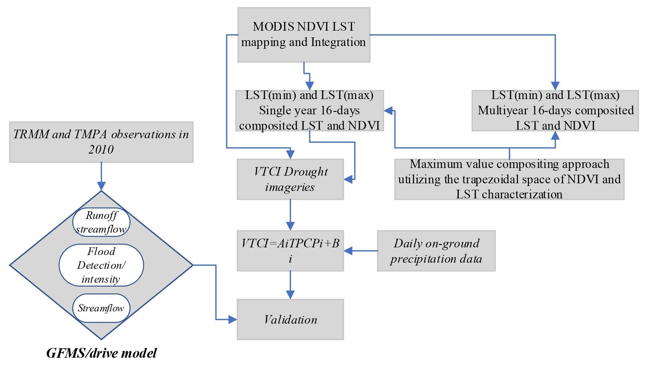
2. Study Area
3. Materials and Method
3.1. Datasets
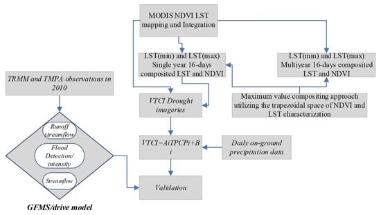
3.2. Methods
4. Results and Discussion
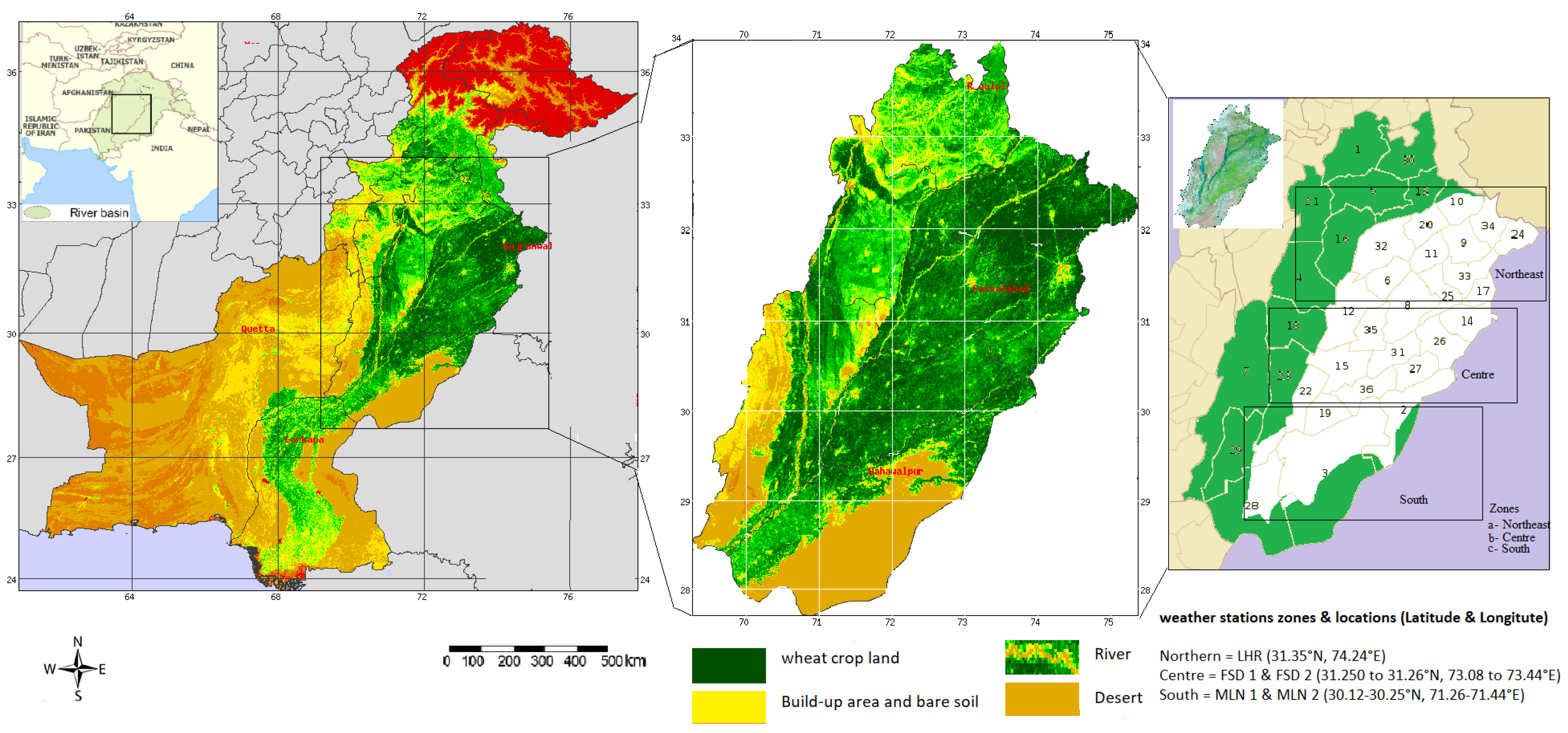
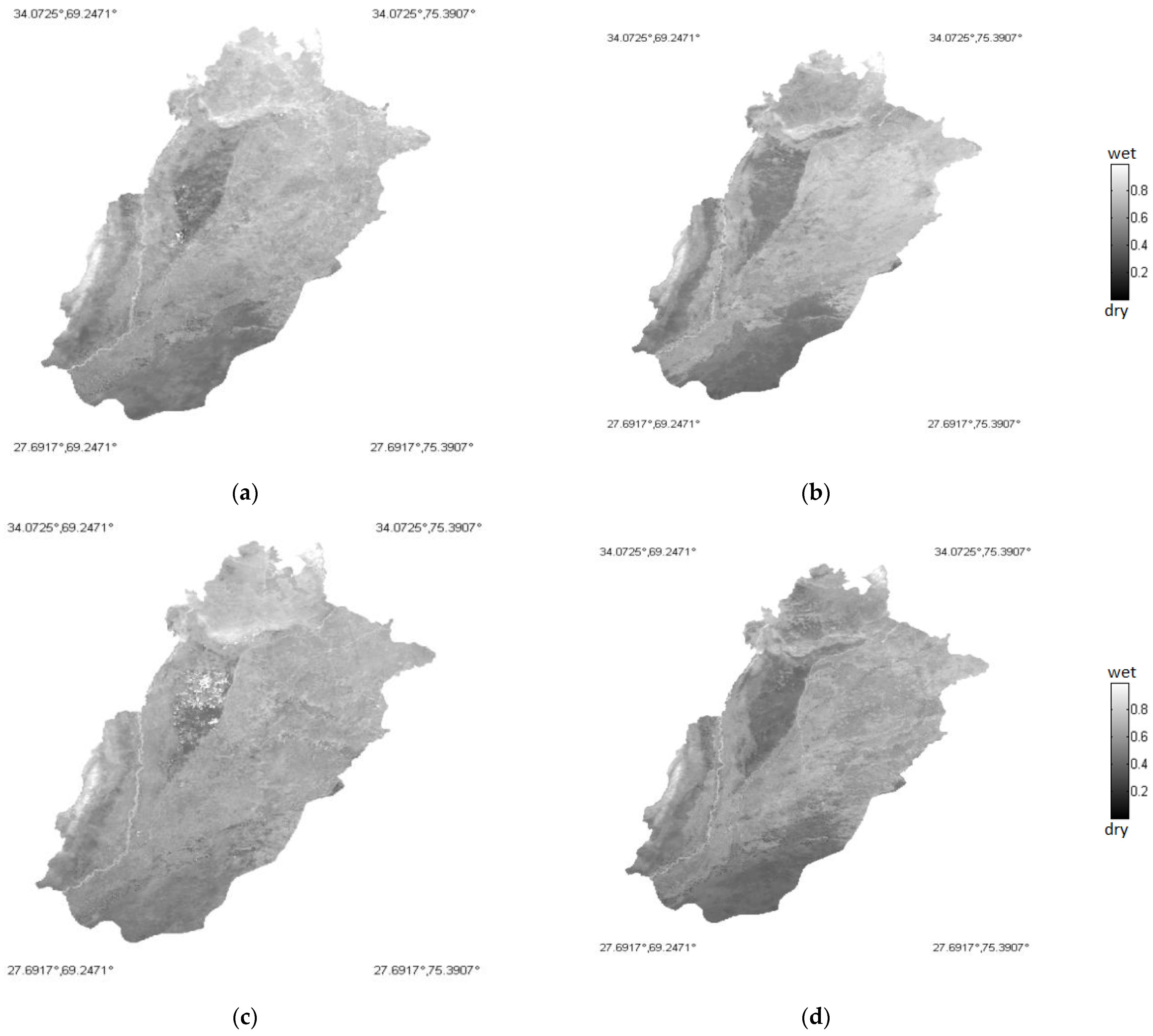
4.1. VTCI Drought, Warm and Cold Edges
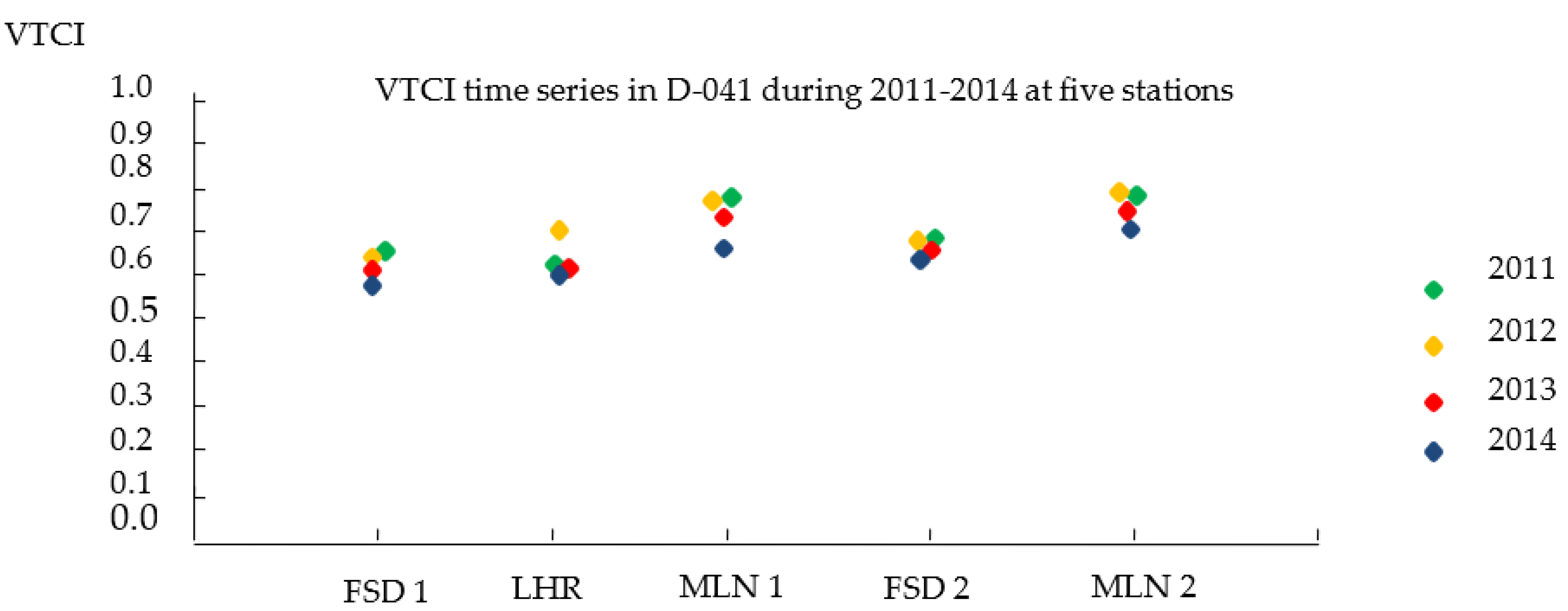
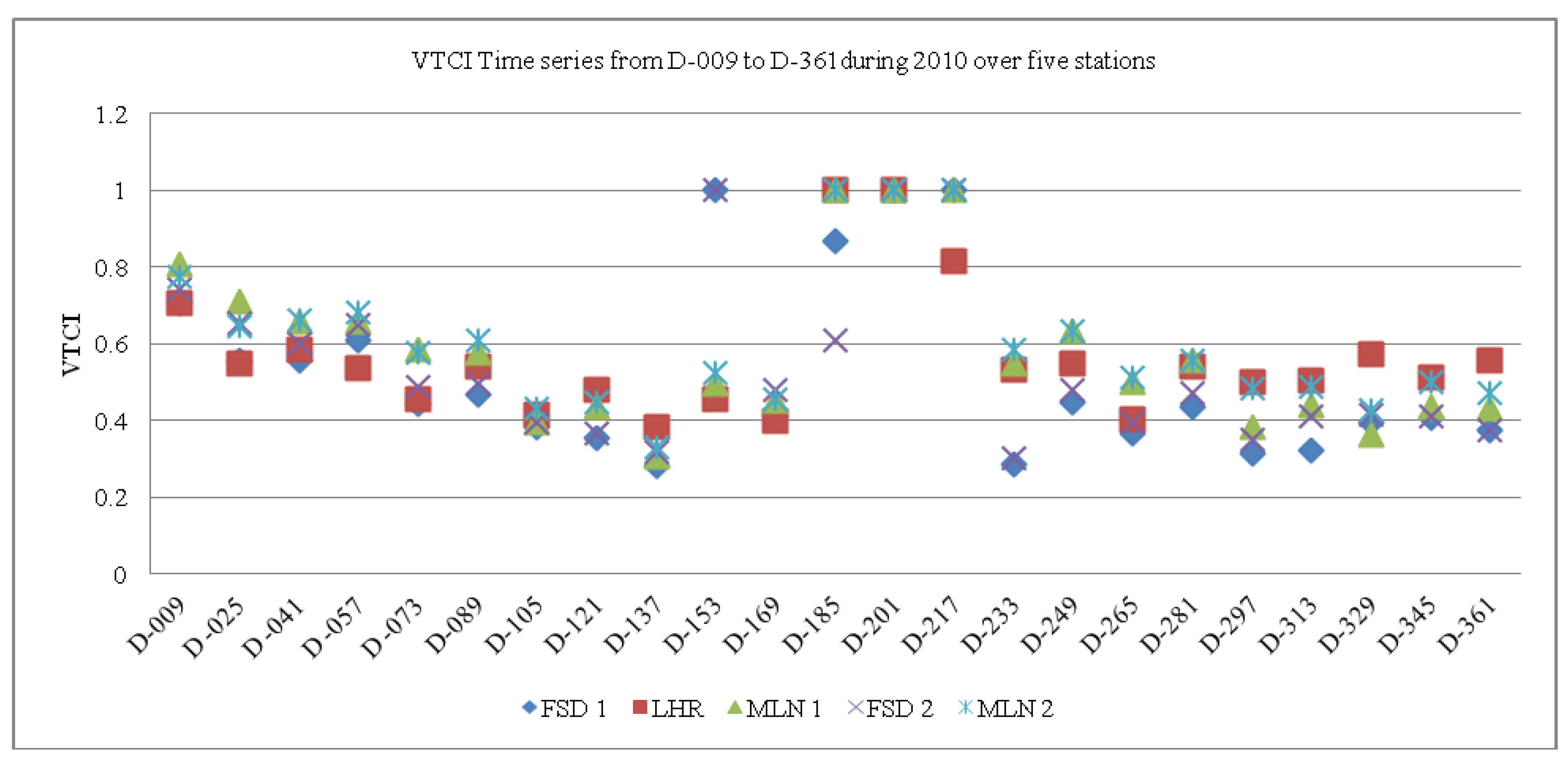
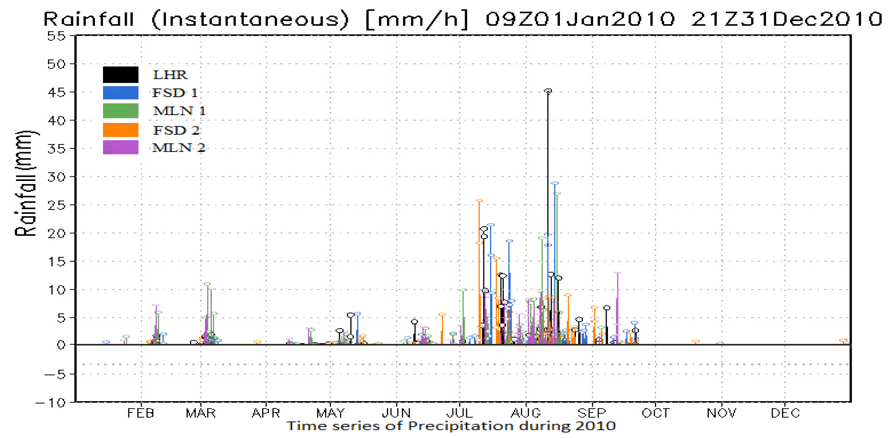
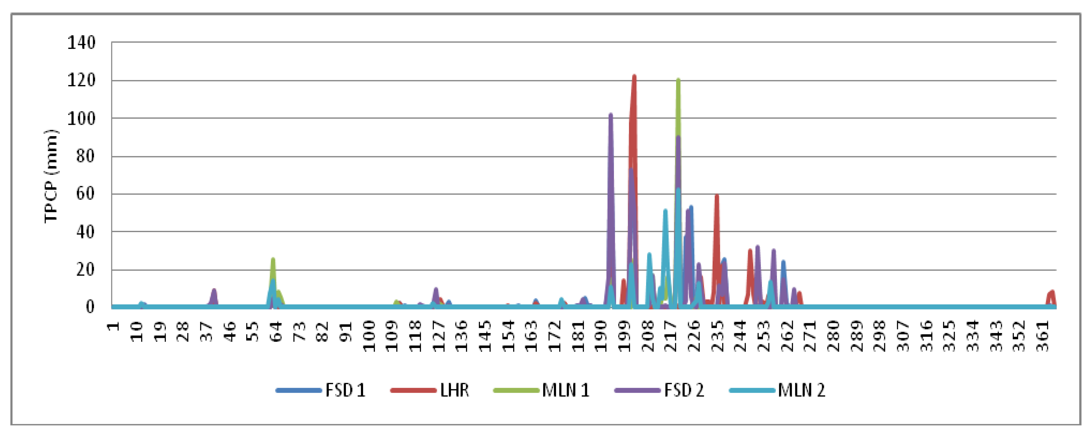
4.2. Time Series Drought and Flood Determination
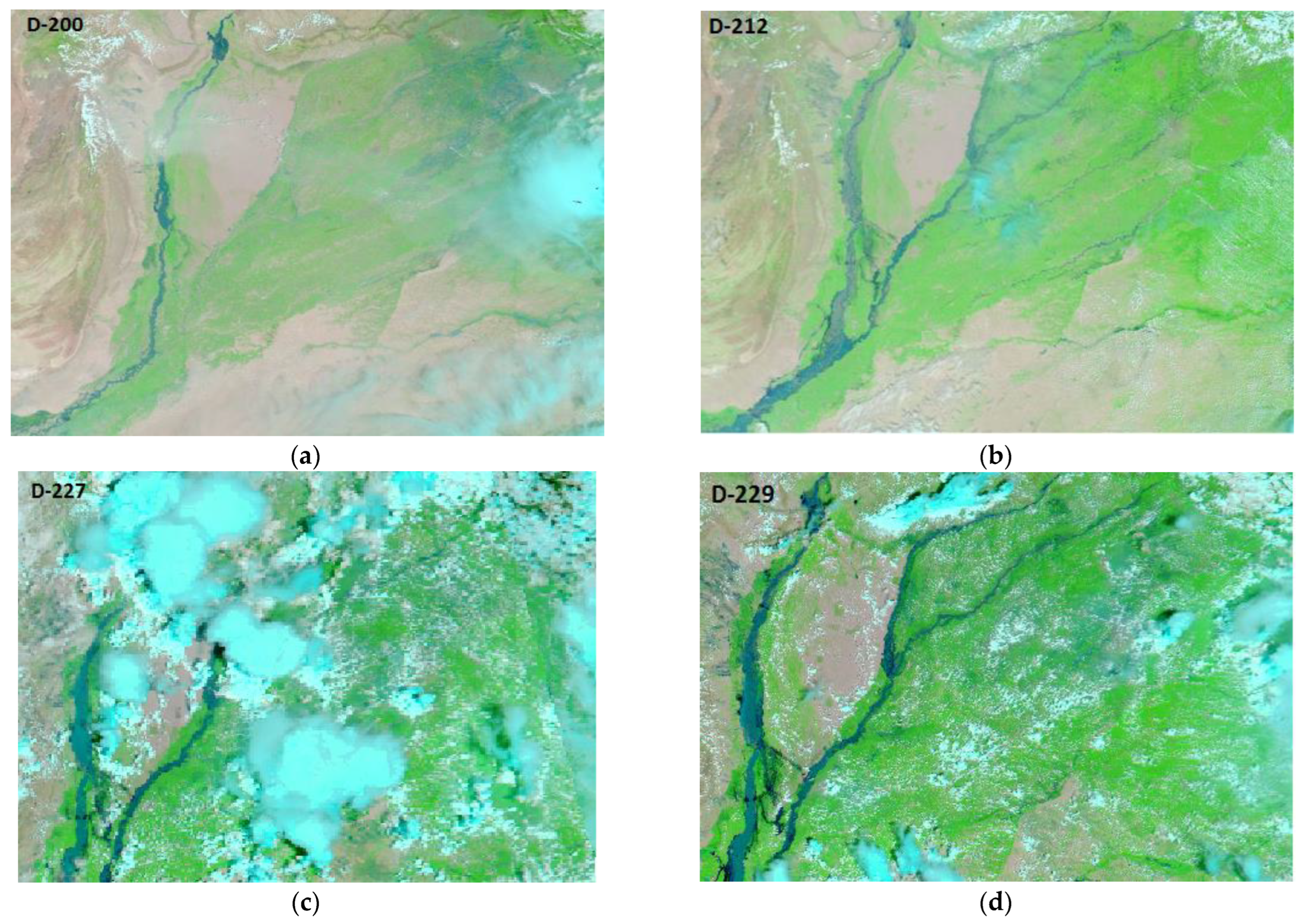
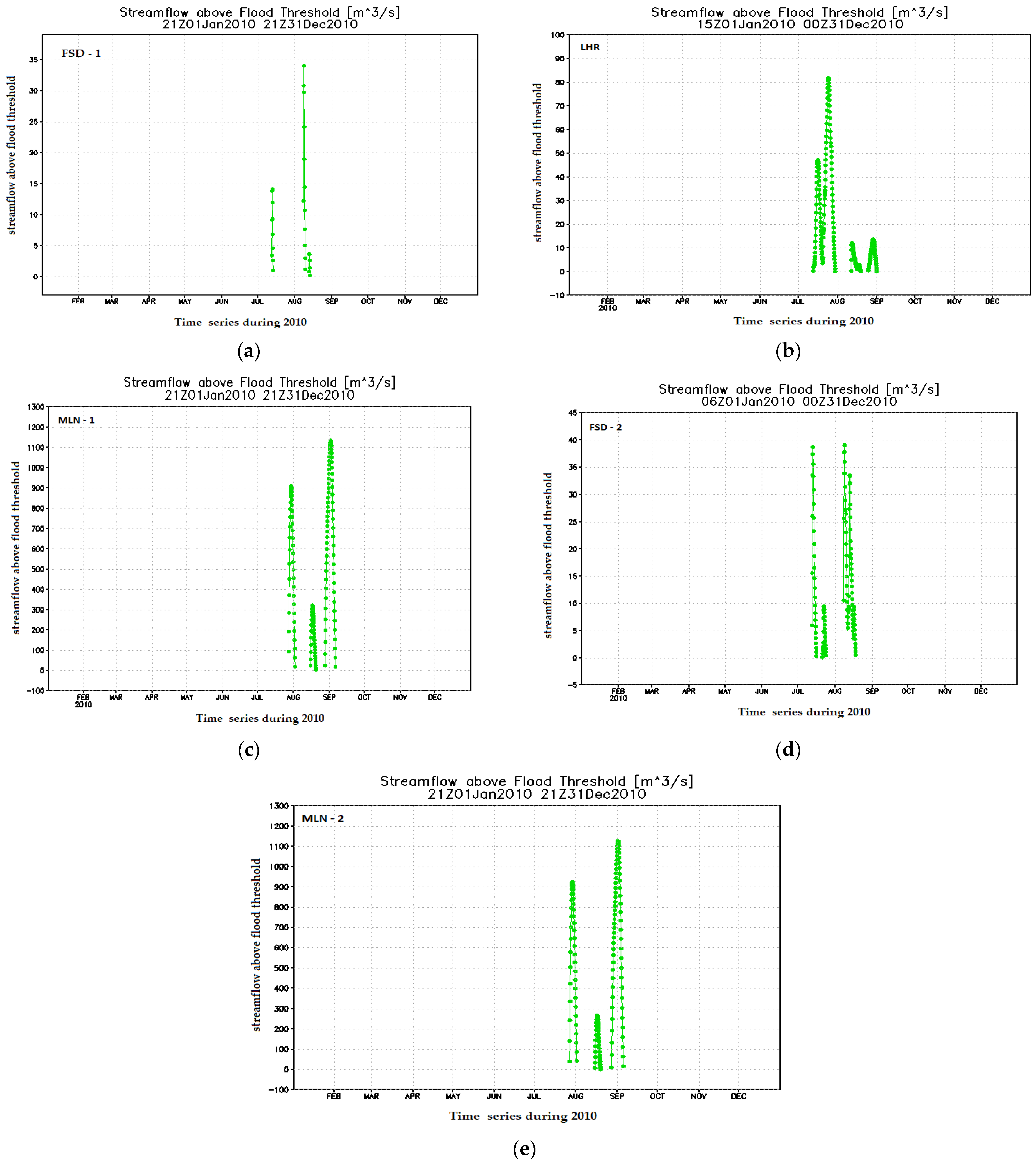
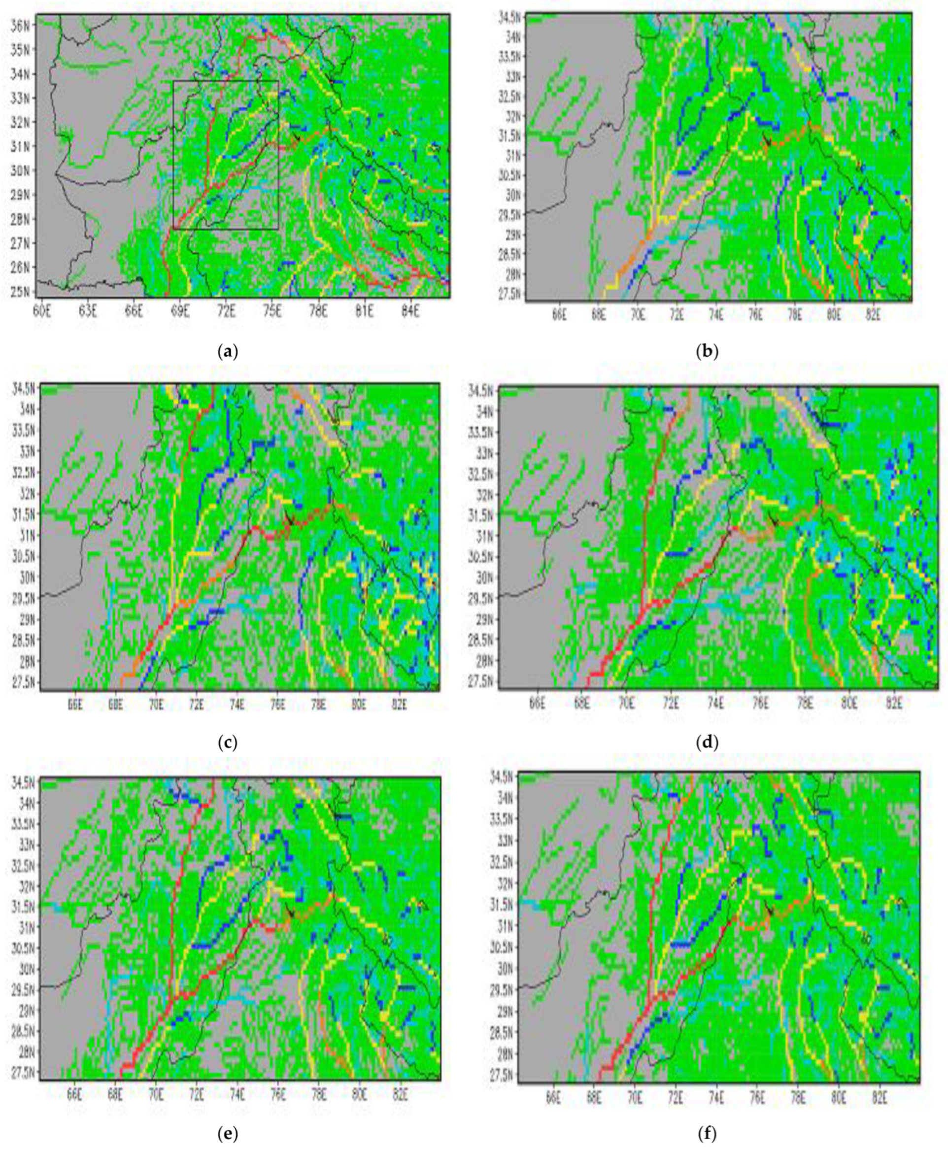
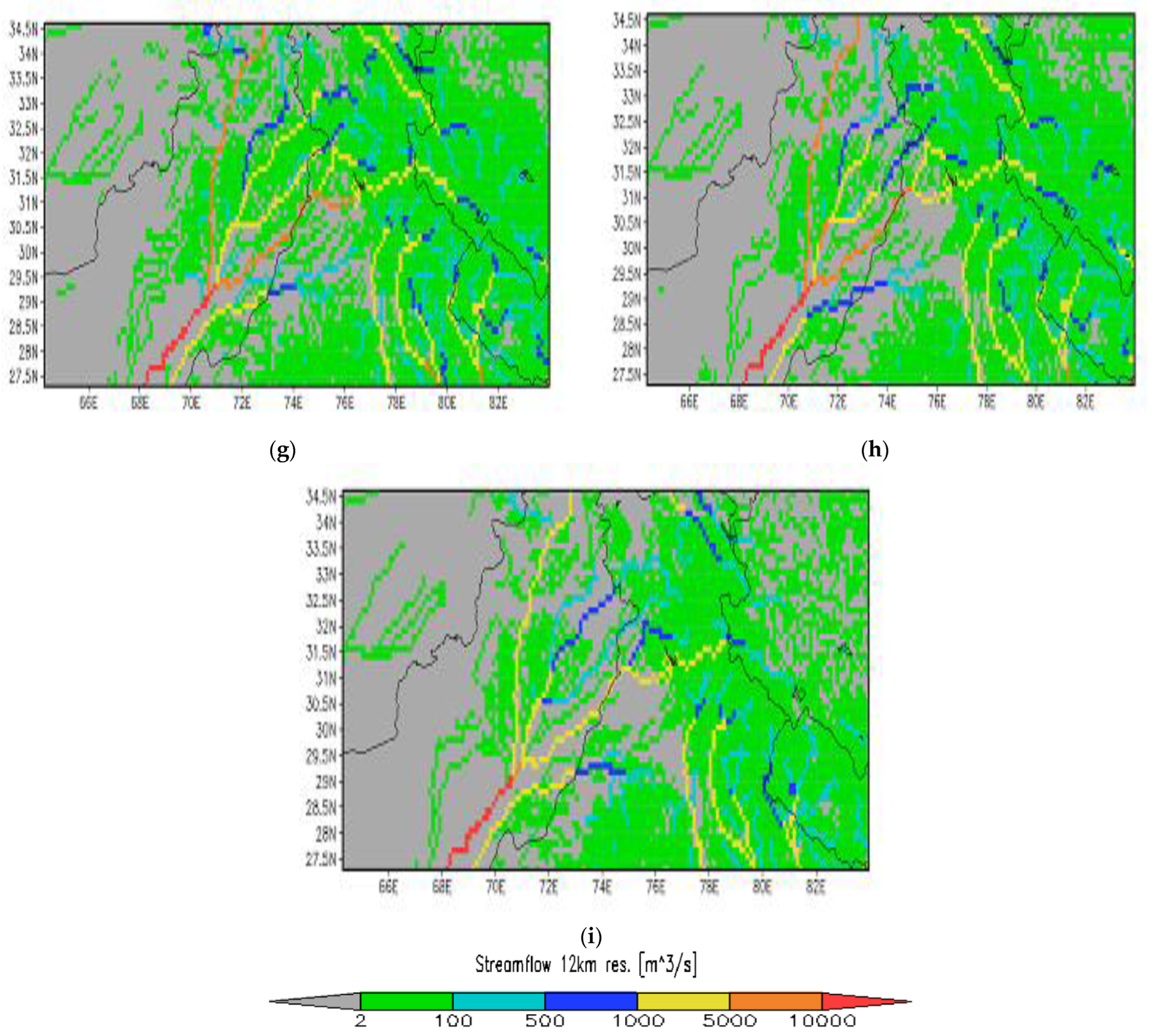
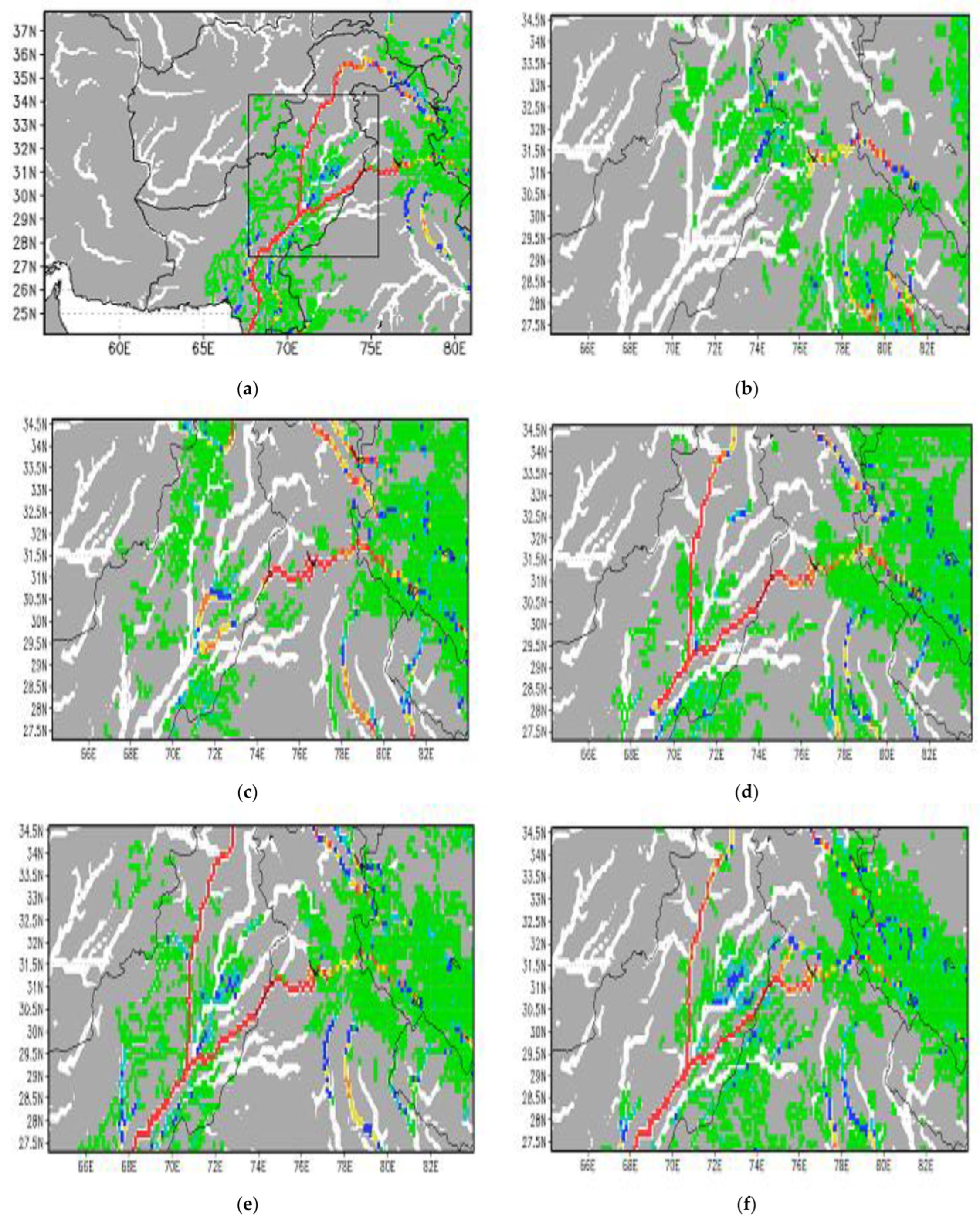
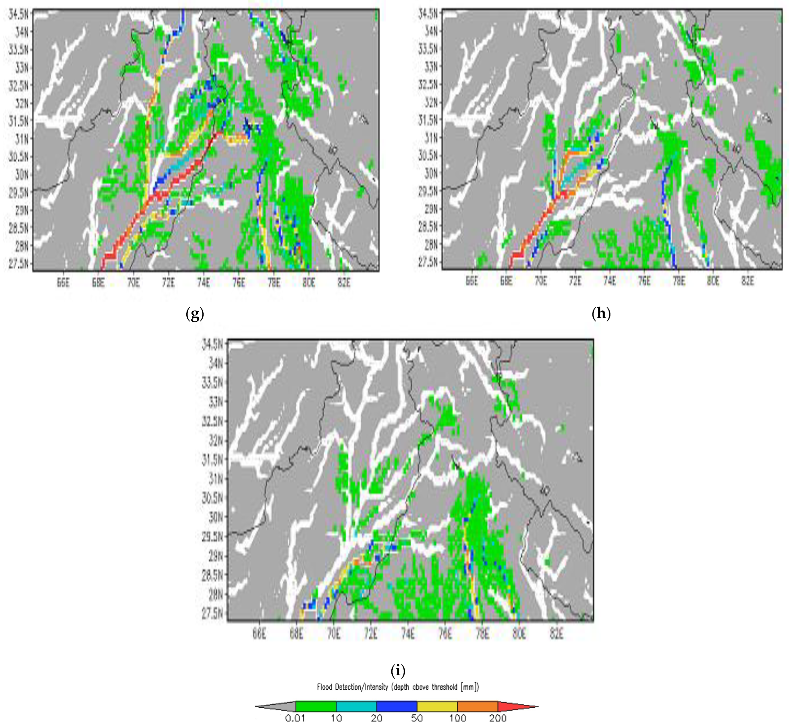
4.3. Determination of Flood Using GFMS Model
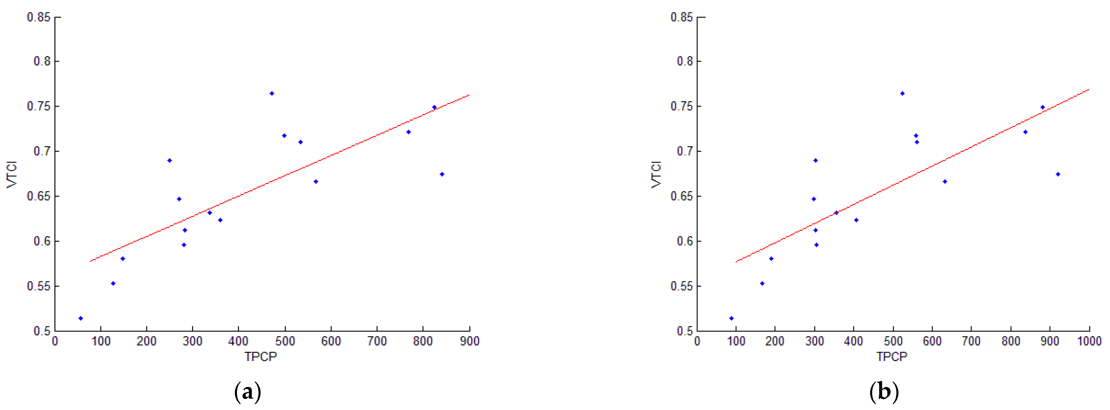
4.4. Validation of Flood and Drought
5. Conclusions
Author Contributions
Funding
Data Availability Statement
Conflicts of Interest
References
- Sorooshian, S.; AghaKouchak, A.; Arkin, P.; Eylander, J.; Foufoula-Georgiou, E.; Harmon, R.; Hendrickx, J.M.H.; Imam, B.; Kuligowski, R.; Skahill, B.; et al. Advancing the Remote Sensing of Precipitation. Bull. Am. Meteorol. Soc. 2011, 92, 1271–1272. [Google Scholar] [CrossRef]
- Shahzaman, M.; Zhu, W.; Bilal, M.; Habtemicheal, B.; Mustafa, F.; Arshad, M.; Ullah, I.; Ishfaq, S.; Iqbal, R. Remote Sensing Indices for Spatial Monitoring of Agricultural Drought in South Asian Countries. Remote Sens. 2021, 13, 2059. [Google Scholar] [CrossRef]
- Shahzaman, M.; Zhu, W.; Ullah, I.; Mustafa, F.; Bilal, M.; Ishfaq, S.; Nisar, S.; Arshad, M.; Iqbal, R.; Aslam, R.W. Comparison of Multi-Year Reanalysis, Models, and Satellite Remote Sensing Products for Agricultural Drought Monitoring over South Asian Countries. Remote Sens. 2021, 13, 3294. [Google Scholar] [CrossRef]
- Tanaka, M.; Sugimura, T.; Tanaka, S.; Tamai, N. Flood–drought cycle of Tonle Sap and Mekong Delta area observed by DMSP-SSM/I. Int. J. Remote Sens. 2003, 24, 1487–1504. [Google Scholar] [CrossRef]
- Jin, Y.-Q. A flooding index and its regional threshold value for monitoring floods in China from SSM/I data. Int. J. Remote Sens. 1999, 20, 1025–1030. [Google Scholar] [CrossRef]
- Rahimi, S.; Gholami Sefidkouhi, M.A.; Raeini-Sarjaz, M.; Valipour, M. Estimation of actual evapotranspiration by using MODIS images (a case study: Tajan catchment). Arch. Agron. Soil Sci. 2015, 61, 695–709. [Google Scholar] [CrossRef]
- Justice, C.O.; Vermote, E.; Townshend, J.R.G.; Defries, R.; Roy, D.P.; Hall, D.K.; Salomonson, V.V.; Privette, J.L.; Riggs, G.; Strahler, A.; et al. The Moderate Resolution Imaging Spectroradiometer (MODIS): Land remote sensing for global change research. IEEE Trans. Geosci. Remote Sens. 1998, 36, 1228–1249. [Google Scholar] [CrossRef] [Green Version]
- Sajjad, M.M.; Wang, J.; Abbas, H.; Ullah, I.; Khan, R.; Ali, F. Impact of Climate and Land-Use Change on Groundwater Resources, Study of Faisalabad District, Pakistan. Atmosphere 2022, 13, 1097. [Google Scholar] [CrossRef]
- Kogan, F.N. Application of vegetation index and brightness temperature for drought detection. Adv. Space Res. 1995, 15, 91–100. [Google Scholar] [CrossRef]
- Lu, E. Determining the start, duration, and strength of flood and drought with daily precipitation: Rationale. Geophys. Res. Lett. 2009, 36, L12707. [Google Scholar] [CrossRef]
- Zargar, A.; Sadiq, R.; Naser, B.; Khan, F.I. A review of drought indices. Environ. Rev. 2011, 19, 333–349. [Google Scholar] [CrossRef] [Green Version]
- Park, S.; Feddema, J.J.; Egbert, S.L. MODIS land surface temperature composite data and their relationships with climatic water budget factors in the central Great Plains. Int. J. Remote Sens. 2005, 26, 1127–1144. [Google Scholar] [CrossRef]
- Liu, W.T.H.; Massambani, O.; Nobre, C.A. Satellite recorded vegetation response to drought in brazil. Int. J. Climatol. 1994, 14, 343–354. [Google Scholar] [CrossRef]
- AghaKouchak, A.; Farahmand, A.; Melton, F.S.; Teixeira, J.; Anderson, M.C.; Wardlow, B.D.; Hain, C.R. Remote sensing of drought: Progress, challenges and opportunities. Rev. Geophys. 2015, 53, 452–480. [Google Scholar] [CrossRef] [Green Version]
- Wilhite, D.A.; Glantz, M.H. Understanding: The Drought Phenomenon: The Role of Definitions. Water Int. 1985, 10, 111–120. [Google Scholar] [CrossRef] [Green Version]
- Palmer, W.C. Meteorological Drought; U.S. Weather Bureau Research Paper No. 45; U.S. Department of Commerce, Weather Bureau: Silver Spring, MD, USA, 1965; Volume 58.
- Byun, H.R.; Wilhite, D.A. Objective quantification of drought severity and duration. J. Clim. 1999, 12, 2747–2756. [Google Scholar] [CrossRef]
- Dai, A. Drought under global warming: A review. WIREs Clim. Chang. 2011, 2, 45–65. [Google Scholar] [CrossRef] [Green Version]
- Ullah, I.; Ma, X.; Yin, J.; Asfaw, T.; Azam, K.; Syed, S.; Liu, M.; Arshad, M.; Shahzaman, M. Evaluating the meteorological drought characteristics over Pakistan using in situ observations and reanalysis products. Int. J. Climatol. 2021, 41, 4437–4459. [Google Scholar] [CrossRef]
- Ullah, I.; Ma, X.; Yin, J.; Saleem, F.; Syed, S.; Omer, A.; Habtemicheal, B.A.; Liu, M.; Arshad, M. Observed changes in seasonal drought characteristics and their possible potential drivers over Pakistan. Int. J. Climatol. 2022, 42, 1576–1596. [Google Scholar] [CrossRef]
- Ali, M.; Ghaith, M.; Wagdy, A.; Helmi, A.M. Development of a New Multivariate Composite Drought Index for the Blue Nile River Basin. Water 2022, 14, 886. [Google Scholar] [CrossRef]
- McKee, T.B.; Nolan, J.; Kleist, J. The relationship of drought frequency and duration to time scales. In Proceedings of the Eighth Conference on Applied Climatology, Anaheim, CA, USA, 17–22 January 1993. [Google Scholar]
- Meng, L.; Shen, Y. On the Relationship of Soil Moisture and Extreme Temperatures in East China. Earth Interact. 2014, 18, 1–20. [Google Scholar] [CrossRef]
- Wan, Z.; Wang, P.; Li, X. Using MODIS Land Surface Temperature and Normalized Difference Vegetation Index products for monitoring drought in the southern Great Plains, USA. Int. J. Remote Sens. 2004, 25, 61–72. [Google Scholar] [CrossRef]
- Dai, A. Increasing drought under global warming in observations and models. Nat. Clim. Chang. 2013, 3, 52–58. [Google Scholar] [CrossRef]
- Dai, A. Characteristics and trends in various forms of the Palmer Drought Severity Index during 1900–2008. J. Geophys. Res. Atmos. 2011, 116. [Google Scholar] [CrossRef] [Green Version]
- Dai, A. Hydroclimatic trends during 1950–2018 over global land. Clim. Dyn. 2021, 56, 4027–4049. [Google Scholar] [CrossRef]
- Zeng, X.; Lu, E. Globally Unified Monsoon Onset and Retreat Indexes. J. Clim. 2004, 17, 2241–2248. [Google Scholar] [CrossRef]
- Findell, K.L.; Berg, A.; Gentine, P.; Krasting, J.P.; Lintner, B.R.; Malyshev, S.; Santanello, J.A.; Shevliakova, E. The impact of anthropogenic land use and land cover change on regional climate extremes. Nat. Commun. 2017, 8, 989. [Google Scholar] [CrossRef] [Green Version]
- Ullah, I.; Ma, X.; Ren, G.; Yin, J.; Iyakaremye, V.; Syed, S.; Lu, K.; Xing, Y.; Singh, V.P. Recent Changes in Drought Events over South Asia and Their Possible Linkages with Climatic and Dynamic Factors. Remote Sens. 2022, 14, 3219. [Google Scholar] [CrossRef]
- Ullah, I.; Ma, X.; Yin, J.; Omer, A.; Habtemicheal, B.A.; Saleem, F.; Iyakaremye, V.; Syed, S.; Arshad, M.; Liu, M. Spatiotemporal characteristics of meteorological drought variability and trends (1981–2020) over South Asia and the associated large-scale circulation patterns. Clim. Dyn. 2022. [Google Scholar] [CrossRef]
- Sun, W.; Wang, P.-X.; Zhang, S.-Y.; Zhu, D.-H.; Liu, J.-M.; Chen, J.-H.; Yang, H.-S. Using the vegetation temperature condition index for time series drought occurrence monitoring in the Guanzhong Plain, PR China. Int. J. Remote Sens. 2008, 29, 5133–5144. [Google Scholar] [CrossRef]
- BAI, J.; YU, Y.; Di, L. Comparison between TVDI and CWSI for drought monitoring in the Guanzhong Plain, China. J. Integr. Agric. 2017, 16, 389–397. [Google Scholar] [CrossRef] [Green Version]
- Gao, Z.; Wang, Q.; Cao, X.; Gao, W. The responses of vegetation water content (EWT) and assessment of drought monitoring along a coastal region using remote sensing. GIScience Remote Sens. 2014, 51, 1–16. [Google Scholar] [CrossRef]
- Wang, L.; Qu, J.J. NMDI: A normalized multi-band drought index for monitoring soil and vegetation moisture with satellite remote sensing. Geophys. Res. Lett. 2007, 34, L20405. [Google Scholar] [CrossRef]
- Peters, A.J.; Walter-Shea, E.A.; Ji, L.; Viña, A.; Hayes, M.; Svoboda, M.D. Drought monitoring with NDVI-based Standardized Vegetation Index. Photogramm. Eng. Remote Sens. 2002, 68, 71–75. [Google Scholar]
- Parviz, L. Determination of effective indices in the drought monitoring through analysis of satellite images. J. Agric. For. 2016, 62, 305–324. [Google Scholar] [CrossRef] [Green Version]
- Ma, X.; Yoshikane, T.; Hara, M.; Wakazuki, Y.; Takahashi, H.G.; Kimura, F. Hydrological response to future climate change in the Agano River basin, Japan. Hydrol. Res. Lett. 2010, 4, 25–29. [Google Scholar] [CrossRef] [Green Version]
- Ma, X.; Fukushima, Y. A numerical model of the river freezing process and its application to the Lena River. Hydrol. Process. 2002, 16, 2131–2140. [Google Scholar] [CrossRef]
- Zhou, H.; Zhou, W.; Liu, Y.; Yuan, Y.; Huang, J.; Liu, Y. Meteorological Drought Migration in the Poyang Lake Basin, China: Switching among Different Climate Modes. J. Hydrometeorol. 2020, 21, 415–431. [Google Scholar] [CrossRef]
- Han, Y.; Wang, Y.; Zhao, Y. Estimating Soil Moisture Conditions of the Greater Changbai Mountains by Land Surface Temperature and NDVI. IEEE Trans. Geosci. Remote Sens. 2010, 48, 2509–2515. [Google Scholar] [CrossRef]
- Goetz, S.J. Multi-sensor analysis of NDVI, surface temperature and biophysical variables at a mixed grassland site. Int. J. Remote Sens. 1997, 18, 71–94. [Google Scholar] [CrossRef]
- Coll, C.; Hook, S.J.; Galve, J.M. Land Surface Temperature From the Advanced Along-Track Scanning Radiometer: Validation Over Inland Waters and Vegetated Surfaces. IEEE Trans. Geosci. Remote Sens. 2009, 47, 350–360. [Google Scholar] [CrossRef]
- Adnan, S.; Ullah, K.; Shouting, G. Investigations into precipitation and drought climatologies in south central Asia with special focus on Pakistan over the period 1951-2010. J. Clim. 2016, 29, 6019–6035. [Google Scholar] [CrossRef]
- Hina, S.; Saleem, F.; Arshad, A.; Hina, A.; Ullah, I. Droughts over Pakistan: Possible cycles, precursors and associated mechanisms. Geomat. Nat. Hazards Risk 2021, 12, 1638–1668. [Google Scholar] [CrossRef]
- Sein, Z.M.M.; Ullah, I.; Iyakaremye, V.; Azam, K.; Ma, X.; Syed, S.; Zhi, X. Observed spatiotemporal changes in air temperature, dew point temperature and relative humidity over Myanmar during 2001–2019. Meteorol. Atmos. Phys. 2022, 134, 7. [Google Scholar] [CrossRef]
- Sein, Z.M.M.; Zhi, X.; Ullah, I.; Azam, K.; Ngoma, H.; Saleem, F.; Xing, Y.; Iyakaremye, V.; Syed, S.; Hina, S.; et al. Recent variability of sub-seasonal monsoon precipitation and its potential drivers in Myanmar using in-situ observation during 1981–2020. Int. J. Climatol. 2022, 42, 3341–3359. [Google Scholar] [CrossRef]
- Mie Sein, Z.M.; Ullah, I.; Saleem, F.; Zhi, X.; Syed, S.; Azam, K. Interdecadal Variability in Myanmar Rainfall in the Monsoon Season (May–October) Using Eigen Methods. Water 2021, 13, 729. [Google Scholar] [CrossRef]
- Mie Sein, Z.; Ullah, I.; Syed, S.; Zhi, X.; Azam, K.; Rasool, G. Interannual Variability of Air Temperature over Myanmar: The Influence of ENSO and IOD. Climate 2021, 9, 35. [Google Scholar] [CrossRef]
- Sheikh, M.M.; Manzoor, N.; Ashraf, J.; Adnan, M.; Collins, D.; Hameed, S.; Manton, M.J.; Ahmed, A.U.; Baidya, S.K.; Borgaonkar, H.P.; et al. Trends in extreme daily rainfall and temperature indices over South Asia. Int. J. Climatol. 2015, 35, 1625–1637. [Google Scholar] [CrossRef]
- Ahmed, K.; Shahid, S.; Chung, E.S.; Wang, X.J.; Harun, S.B. Climate change uncertainties in seasonal drought severity-area-frequency curves: Case of arid region of Pakistan. J. Hydrol. 2019, 570, 473–485. [Google Scholar] [CrossRef]
- Arshad, M.; Ma, X.; Yin, J.; Ullah, W.; Ali, G.; Ullah, S.; Liu, M.; Shahzaman, M.; Ullah, I. Evaluation of GPM-IMERG and TRMM-3B42 precipitation products over Pakistan. Atmos. Res. 2021, 249, 105341. [Google Scholar] [CrossRef]
- Arshad, M.; Ma, X.; Yin, J.; Ullah, W.; Liu, M.; Ullah, I. Performance evaluation of ERA-5, JRA-55, MERRA-2, and CFS-2 reanalysis datasets, over diverse climate regions of Pakistan. Weather Clim. Extrem. 2021, 33, 100373. [Google Scholar] [CrossRef]
- Xing, Y.; Shao, D.; Liang, Q.; Chen, H.; Ma, X.; Ullah, I. Investigation of the drainage loss effects with a street view based drainage calculation method in hydrodynamic modelling of pluvial floods in urbanized area. J. Hydrol. 2022, 605, 127365. [Google Scholar] [CrossRef]
- Liu, M.; Ma, X.; Yin, Y.; Zhang, Z.; Yin, J.; Ullah, I.; Arshad, M. Non-stationary frequency analysis of extreme streamflow disturbance in a typical ecological function reserve of China under a changing climate. Ecohydrology 2021, 23, e2323. [Google Scholar] [CrossRef]
- Iyakaremye, V.; Zeng, G.; Yang, X.; Zhang, G.; Ullah, I.; Gahigi, A.; Vuguziga, F.; Asfaw, T.; Ayugi, B. Increased high-temperature extremes and associated population exposure in Africa by the mid-21st century. Sci. Total Environ. 2021, 790, 148162. [Google Scholar] [CrossRef]
- Uwimbabazi, J.; Jing, Y.; Iyakaremye, V.; Ullah, I.; Ayugi, B. Observed Changes in Meteorological Drought Events during 1981–2020 over Rwanda, East Africa. Sustainability 2022, 14, 1519. [Google Scholar] [CrossRef]
- Tian, M.; Wang, P.; Khan, J. Drought Forecasting with Vegetation Temperature Condition Index Using ARIMA Models in the Guanzhong Plain. Remote Sens. 2016, 8, 690. [Google Scholar] [CrossRef] [Green Version]
- Wu, H.; Adler, R.F.; Tian, Y.; Huffman, G.J.; Li, H.; Wang, J. Real-time global flood estimation using satellite-based precipitation and a coupled land surface and routing model. Water Resour. Res. 2014, 50, 2693–2717. [Google Scholar] [CrossRef] [Green Version]
- Ullah, I.; Ma, X.; Asfaw, T.G.; Yin, J.; Iyakaremye, V.; Saleem, F.; Xing, Y.; Azam, K.; Syed, S. Projected Changes in Increased Drought Risks Over South Asia Under a Warmer Climate. Earth’s Future 2022, 10, e2022EF002830. [Google Scholar] [CrossRef]
- Ullah, I.; Saleem, F.; Iyakaremye, V.; Yin, J.; Ma, X.; Syed, S.; Hina, S.; Asfaw, T.G.; Omer, A. Projected Changes in Socioeconomic Exposure to Heatwaves in South Asia Under Changing Climate. Earth’s Future 2022, 10, e2021EF002240. [Google Scholar] [CrossRef]
- Hassan, M.; Du, P.; Mahmood, R.; Jia, S.; Iqbal, W. Streamflow response to projected climate changes in the Northwestern Upper Indus Basin based on regional climate model (RegCM4.3) simulation. J. Hydro-Environ. Res. 2019, 27, 32–49. [Google Scholar] [CrossRef]
- Iyakaremye, V.; Zeng, G.; Ullah, I.; Gahigi, A.; Mumo, R.; Ayugi, B. Recent Observed Changes in Extreme High-Temperature Events and Associated Meteorological Conditions over Africa. Int. J. Climatol. 2022, 42, 4522–4537. [Google Scholar] [CrossRef]
- Wu, J.; Chen, X. Spatiotemporal trends of dryness/wetness duration and severity: The respective contribution of precipitation and temperature. Atmos. Res. 2019, 216, 176–185. [Google Scholar] [CrossRef]
- Wu, J.; Chen, X.; Yu, Z.; Yao, H.; Li, W.; Zhang, D. Assessing the impact of human regulations on hydrological drought development and recovery based on a ‘simulated-observed’ comparison of the SWAT model. J. Hydrol. 2019, 577, 123990. [Google Scholar] [CrossRef]
- Lu, K.; Arshad, M.; Ma, X.; Ullah, I.; Wang, J.; Shao, W. Evaluating observed and future spatiotemporal changes in precipitation and temperature across China based on CMIP6-GCMs. Int. J. Climatol. 2022, 42, 7703–7729. [Google Scholar] [CrossRef]


| DOY | Cold Edges | Warm Edges |
|---|---|---|
| 009 | LSTNDVIi min = 287 + 0 × NDVIi | LSTNDVIi max = 319 − 25 × NDVIi |
| 025 | LSTNDVIi min = 287 + 0 × NDVIi | LSTNDVIi max = 320 − 19 × NDVIi |
| 041 | LSTNDVIi min = 287 + 0 × NDVIi | LSTNDVIi max = 322 − 22 × NDVIi |
| 057 | LSTNDVIi min = 292 + 0 × NDVIi | LSTNDVIi max = 330 − 30 × NDVIi |
| 073 | LSTNDVIi min = 294 + 0 × NDVIi | LSTNDVIi max = 330 − 25 × NDVIi |
| 089 | LSTNDVIi min = 298 + 0 × NDVIi | LSTNDVIi max = 341 − 30 × NDVIi |
| 105 | LSTNDVIi min = 298 + 0 × NDVIi | LSTNDVIi max = 341 − 30 × NDVIi |
| 121 | LSTNDVIi min = 300 + 0 × NDVIi | LSTNDVIi max = 341 − 30 × NDVIi |
| 137 | LSTNDVIi min = 300 + 0 × NDVIi | LSTNDVIi max = 341 − 30 × NDVIi |
| 153 | LSTNDVIi min = 300 + 0 × NDVIi | LSTNDVIi max = 350 − 39 × NDVIi |
| 169 | LSTNDVIi min = 300 + 0 × NDVIi | LSTNDVIi max = 350 − 31 × NDVIi |
| 185 | LSTNDVIi min = 298 + 0 × NDVIi | LSTNDVIi max = 338 − 26 × NDVIi |
| 201 | LSTNDVIi min = 290 + 0 × NDVIi | LSTNDVIi max = 330 − 25 × NDVIi |
| 217 | LSTNDVIi min = 285 + 0 × NDVIi | LSTNDVIi max = 330 − 25 × NDVIi |
| 233 | LSTNDVIi min = 295 + 0 × NDVIi | LSTNDVIi max = 335 − 30 × NDVIi |
| 249 | LSTNDVIi min = 298 + 0 × NDVIi | LSTNDVIi max = 330 − 25 × NDVIi |
| 265 | LSTNDVIi min = 298 + 0 × NDVIi | LSTNDVIi max = 330 − 25 × NDVIi |
| 281 | LSTNDVIi min = 298 + 0 × NDVIi | LSTNDVIi max = 330 − 23 × NDVIi |
| 297 | LSTNDVIi min = 295 + 0 × NDVIi | LSTNDVIi max = 320 − 20 × NDVIi |
| 313 | LSTNDVIi min = 294 + 0 × NDVIi | LSTNDVIi max = 317 − 16 × NDVIi |
| 329 | LSTNDVIi min = 292 + 0 × NDVIi | LSTNDVIi max = 315 − 18 × NDVIi |
| 345 | LSTNDVIi min = 288 + 0 × NDVIi | LSTNDVIi max = 313 − 20 × NDVIi |
| 361 | LSTNDVIi min = 285 + 0 × NDVIi | LSTNDVIi max = 309 − 17 × NDVIi |
| TPCP/VTCI | 16-Days | 1- | 2- | 3- | 4- | 5- | 6- | 9- | 12-Months |
|---|---|---|---|---|---|---|---|---|---|
| D-009 | −0.2370 | −0.2370 | −0.2370 | 0.1902 | 0.7360 | 0.7494 | 0.9484 | 0.9426 | 0.9364 |
| D-025 | 0.7707 | 0.6731 | 0.6731 | 0.7055 | 0.7160 | 0.3573 | 0.4164 | 0.5456 | 0.5881 |
| D-041 | 0.5552 | 0.8509 | 0.8130 | 0.8130 | 0.7930 | 0.8174 | 0.8822 | 0.8706 | 0.8407 |
| D-057 | 0.6663 | 0.6663 | 0.7374 | 0.7374 | 0.7292 | 0.7298 | 0.3822 | −0.2044 | −0.2223 |
| D-073 | - | −0.6777 | −0.5691 | −0.6163 | −0.6163 | −0.6083 | −0.3467 | 0.9356 | 0.9562 |
| D-089 | - | - | −0.5707 | −0.5058 | −0.5058 | −0.4871 | −0.3691 | 0.8096 | 0.8024 |
| D-105 | 0.0579 | 0.0579 | −0.0395 | 0.0494 | 0.0759 | 0.0759 | 0.0544 | 0.2428 | 0.2017 |
| D-121 | 0.6399 | 0.7453 | 0.7453 | −0.5590 | −0.3661 | −0.3661 | −0.3502 | 0.8882 | 0.9767 |
| D-137 | −0.3942 | 0.6505 | 0.6618 | −0.2967 | −0.0898 | −0.0878 | −0.0878 | 0.9864 | 0.7055 |
| D-153 | 0.4068 | 0.3925 | 0.5992 | 0.5992 | −0.1453 | 0.0662 | 0.0662 | 0.9440 | 0.5541 |
| D-169 | −0.2972 | −0.3412 | −0.3553 | −0.2760 | 0.9380 | 0.8019 | 0.9748 | 0.6764 | −0.1636 |
| D-185 | −0.2373 | −0.2278 | −0.2233 | −0.2667 | −0.2667 | −0.4596 | −0.4078 | −0.3914 | −0.2077 |
| D-217 | −0.9365 | −0.5398 | −0.5350 | −0.5330 | −0.5498 | −0.5498 | −0.6216 | −0.6026 | −0.5628 |
| D-233 | 0.8031 | 0.8321 | 0.9555 | 0.9554 | 0.9555 | 0.9577 | 0.9554 | 0.9544 | 0.9046 |
| D-249 | 0.3012 | 0.2084 | 0.3447 | 0.4074 | 0.4109 | 0.4282 | 0.4282 | 0.4531 | 0.4791 |
| D-265 | 0.1182 | 0.5447 | 0.8226 | 0.7347 | 0.7442 | 0.7444 | 0.7460 | 0.7490 | 0.7525 |
| D-281 | 0.3447 | 0.7210 | 0.8607 | 0.9637 | 0.9723 | 0.9743 | 0.9770 | 0.9766 | 0.9741 |
| D-297 | −0.4590 | −0.1984 | 0.6688 | 0.8888 | 0.8922 | 0.8973 | 0.8979 | 0.9000 | 0.8994 |
| D-313 | - | −0.4774 | 0.7258 | 0.8912 | 0.8997 | 0.8910 | 0.8953 | 0.8921 | 0.8920 |
| D-329 | - | - | 0.4081 | 0.5479 | 0.5629 | 0.7039 | 0.7076 | 0.7027 | 0.7024 |
| D-345 | - | - | −0.2688 | 0.7983 | 0.9026 | 0.8481 | 0.8255 | 0.8347 | 0.8356 |
| D-361 | 0.0569 | 0.0569 | 0.0569 | 0.0459 | 0.6350 | 0.8031 | 0.7483 | 0.7382 | 0.7346 |
| TPCP/VTCI | 16-Days | 1- | 2- | 3- | 4- | 5- | 6- | 9- | 12-Months |
|---|---|---|---|---|---|---|---|---|---|
| 009 | 0.5308 | 0.4341 | 0.3376 | 0.3006 | 0.1419 | 0.4322 | 0.224 | 0.3223 | 0.2657 |
| 025 | −0.2478 | −0.0902 | 0.0476 | 0.0559 | 0.0909 | 0.4411 | 0.6262 | 0.6128 | 0.588 |
| 041 | 0.3079 | −0.1691 | −0.0202 | −0.0688 | −0.0635 | −0.0288 | 0.321 | 0.7714 | 0.7694 |
| 057 | 0.2208 | −0.195 | −0.4106 | −0.3219 | −0.3137 | −0.3056 | −0.1252 | 0.367 | 0.3696 |
| 073 | 0.2334 | 0.2127 | −0.0754 | −0.0949 | −0.0672 | −0.0526 | −0.0525 | 0.1128 | 0.1392 |
| 089 | 0.345 | 0.264 | 0.4045 | 0.1507 | 0.2529 | 0.2539 | 0.2702 | 0.5461 | 0.5195 |
| 105 | 0.3296 | 0.3675 | −0.1257 | −0.1394 | −0.0626 | 0.1661 | −0.0048 | 0.1661 | 0.2983 |
| 121 | 0.1713 | 0.4424 | 0.1375 | 0.0969 | −0.2438 | −0.2513 | −0.2476 | 0.0647 | 0.2345 |
| 137 | 0.5405 | 0.7249 | 0.7668 | 0.7139 | 0.4085 | 0.5091 | 0.4717 | 0.2003 | 0.6073 |
| 153 | 0.7177 | 0.7302 | 0.6985 | 0.6019 | 0.7072 | 0.6009 | 0.6209 | 0.5902 | 0.5489 |
| 169 | 0.2930 | 0.2738 | 0.2197 | 0.2374 | 0.158 | 0.1063 | 0.1726 | 0.1785 | 0.3951 |
Disclaimer/Publisher’s Note: The statements, opinions and data contained in all publications are solely those of the individual author(s) and contributor(s) and not of MDPI and/or the editor(s). MDPI and/or the editor(s) disclaim responsibility for any injury to people or property resulting from any ideas, methods, instructions or products referred to in the content. |
© 2023 by the authors. Licensee MDPI, Basel, Switzerland. This article is an open access article distributed under the terms and conditions of the Creative Commons Attribution (CC BY) license (https://creativecommons.org/licenses/by/4.0/).
Share and Cite
Ullah, R.; Khan, J.; Ullah, I.; Khan, F.; Lee, Y. Assessing Impacts of Flood and Drought over the Punjab Region of Pakistan Using Multi-Satellite Data Products. Remote Sens. 2023, 15, 1484. https://doi.org/10.3390/rs15061484
Ullah R, Khan J, Ullah I, Khan F, Lee Y. Assessing Impacts of Flood and Drought over the Punjab Region of Pakistan Using Multi-Satellite Data Products. Remote Sensing. 2023; 15(6):1484. https://doi.org/10.3390/rs15061484
Chicago/Turabian StyleUllah, Rahat, Jahangir Khan, Irfan Ullah, Faheem Khan, and Youngmoon Lee. 2023. "Assessing Impacts of Flood and Drought over the Punjab Region of Pakistan Using Multi-Satellite Data Products" Remote Sensing 15, no. 6: 1484. https://doi.org/10.3390/rs15061484