
Development of High-Resolution Soil Hydraulic Parameters with Use of Earth Observations for Enhancing Root Zone Soil Moisture Product
 , and
, and
Abstract
:1. Introduction
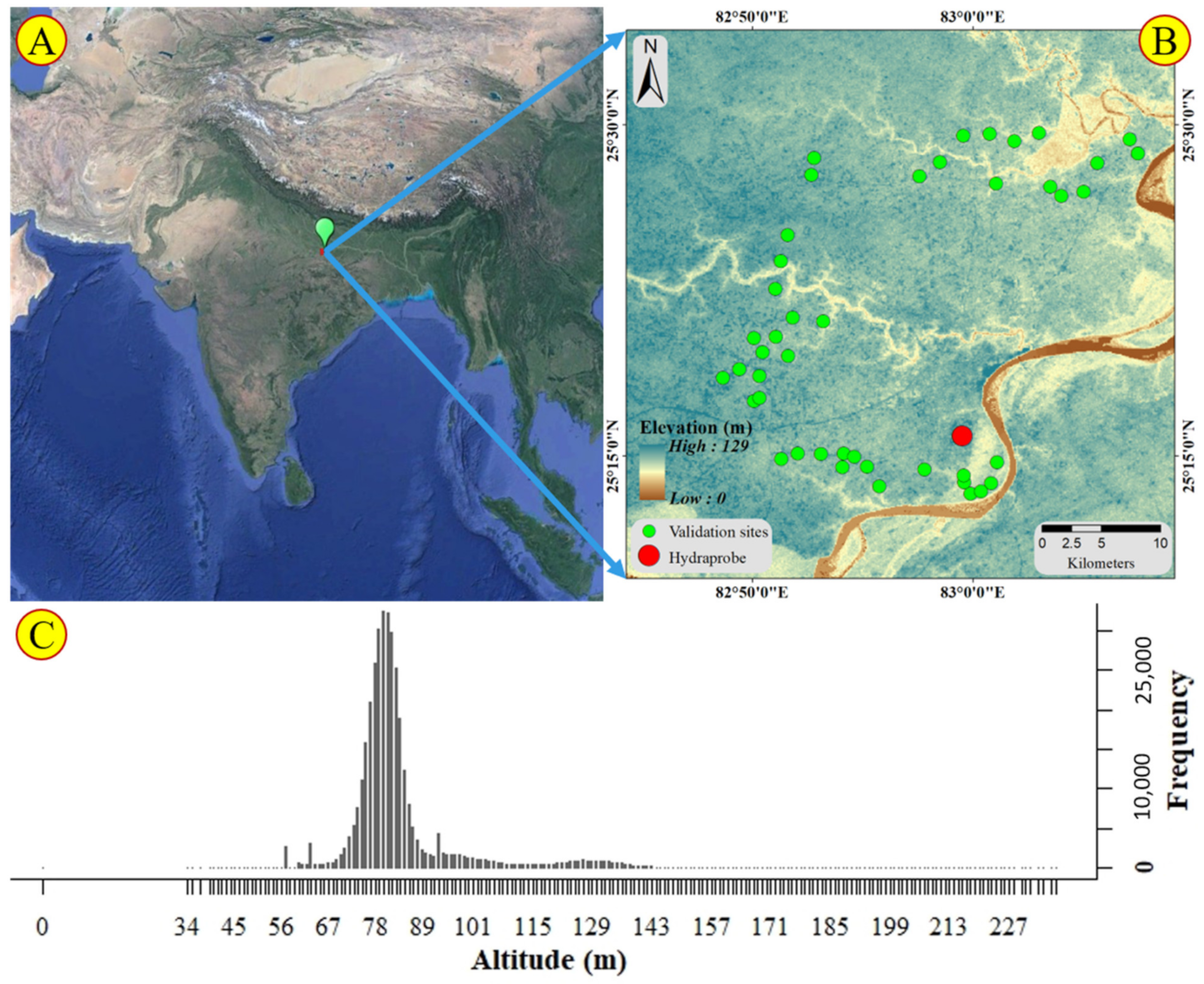
Study Area
2. Data Sources
2.1. In-Situ Soil Moisture Data
2.2. MODIS Data
2.3. C-Band Derived Soil Moisture from AMSR-2
2.4. Field and Ancillary Datasets
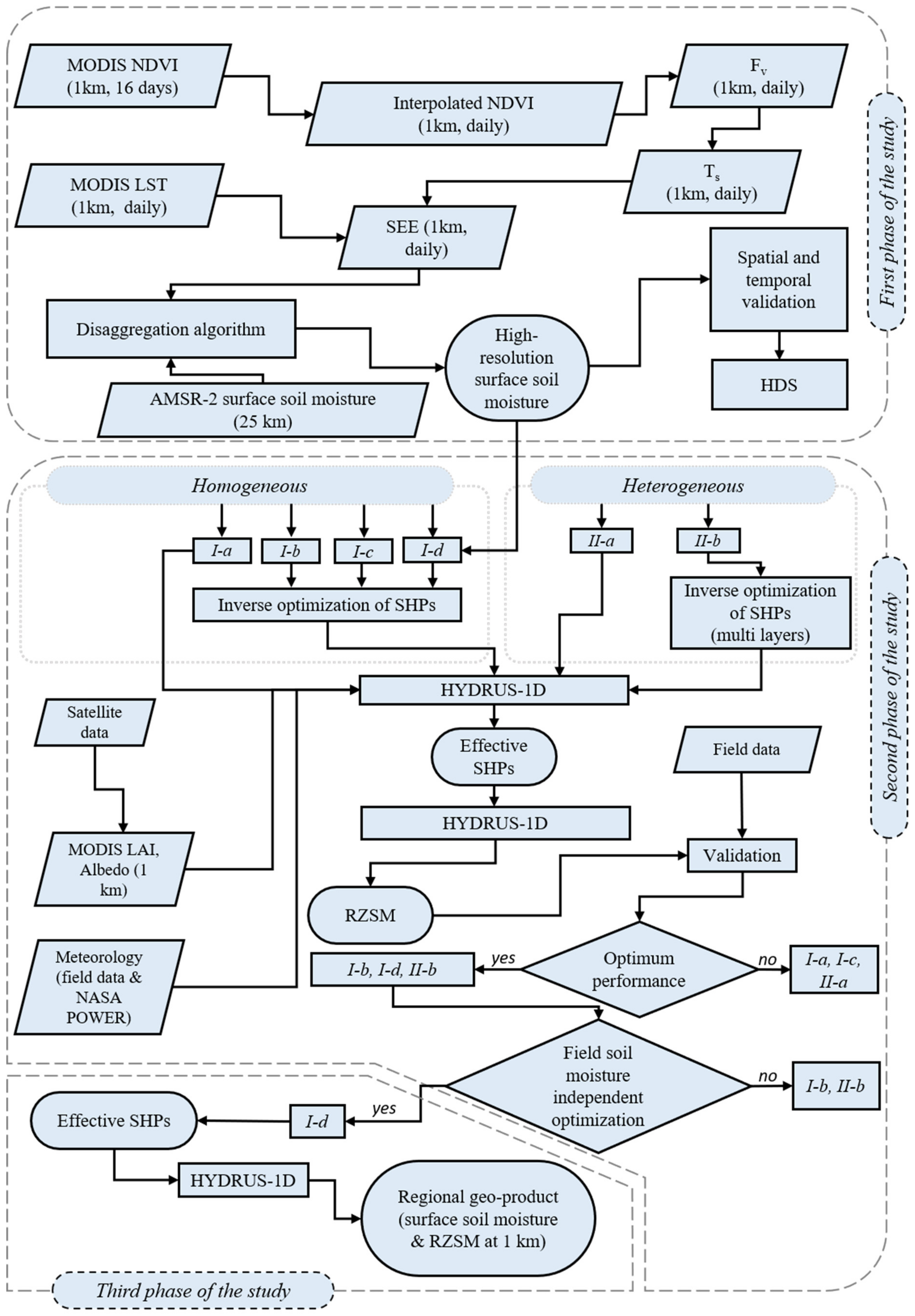
3. Methodology
3.1. Downscaling AMSR-2 Surface Soil Moisture
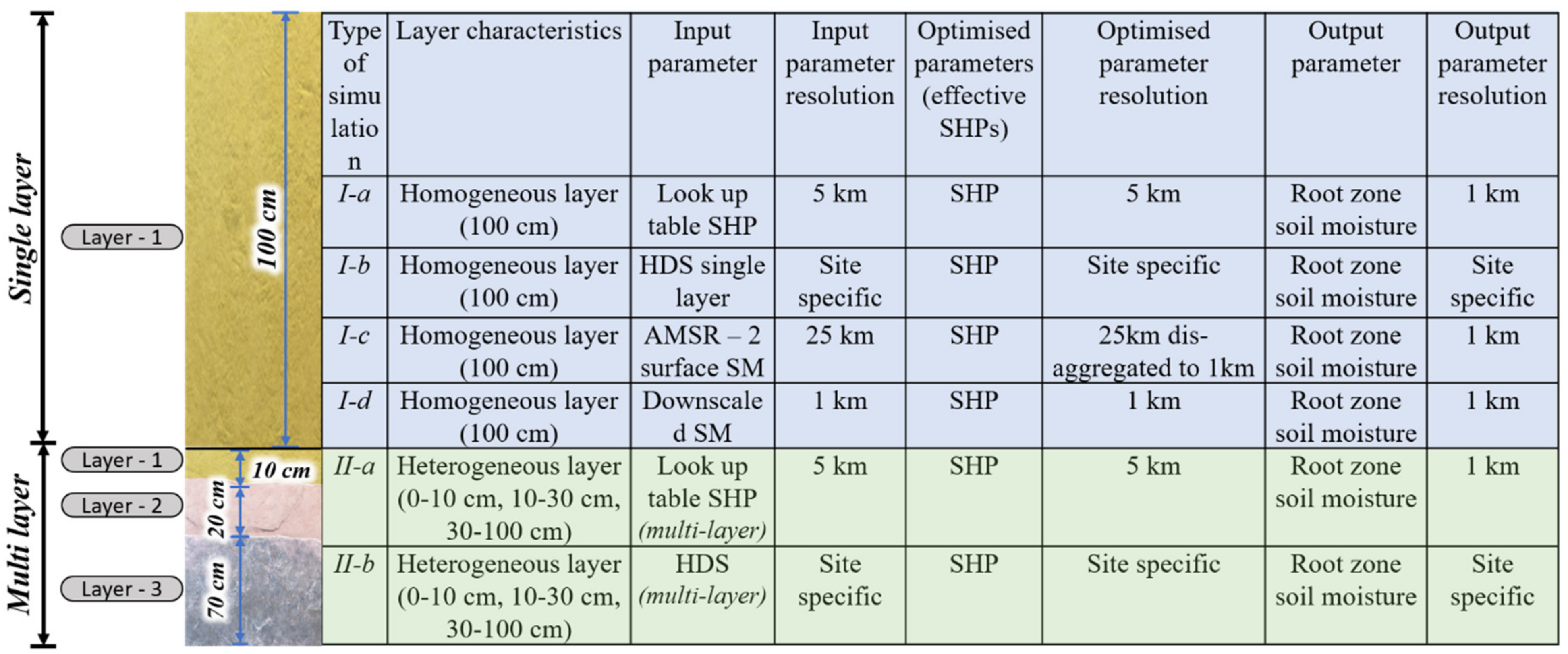
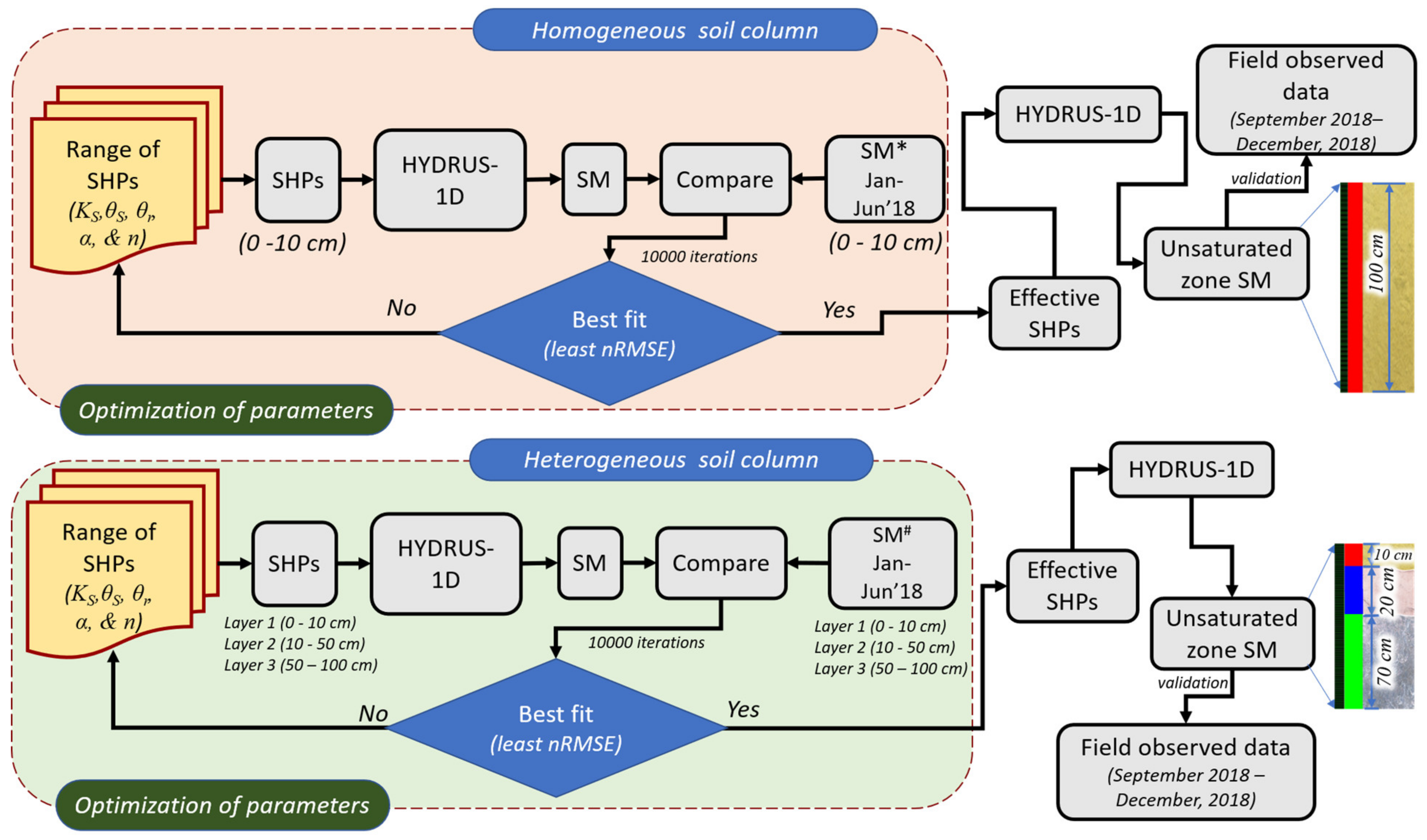
3.2. Derivation of SHPs and RZSM Simulation
Model Initial and Boundary Conditions
3.3. Statistical Analysis for Model Performance
4. Results
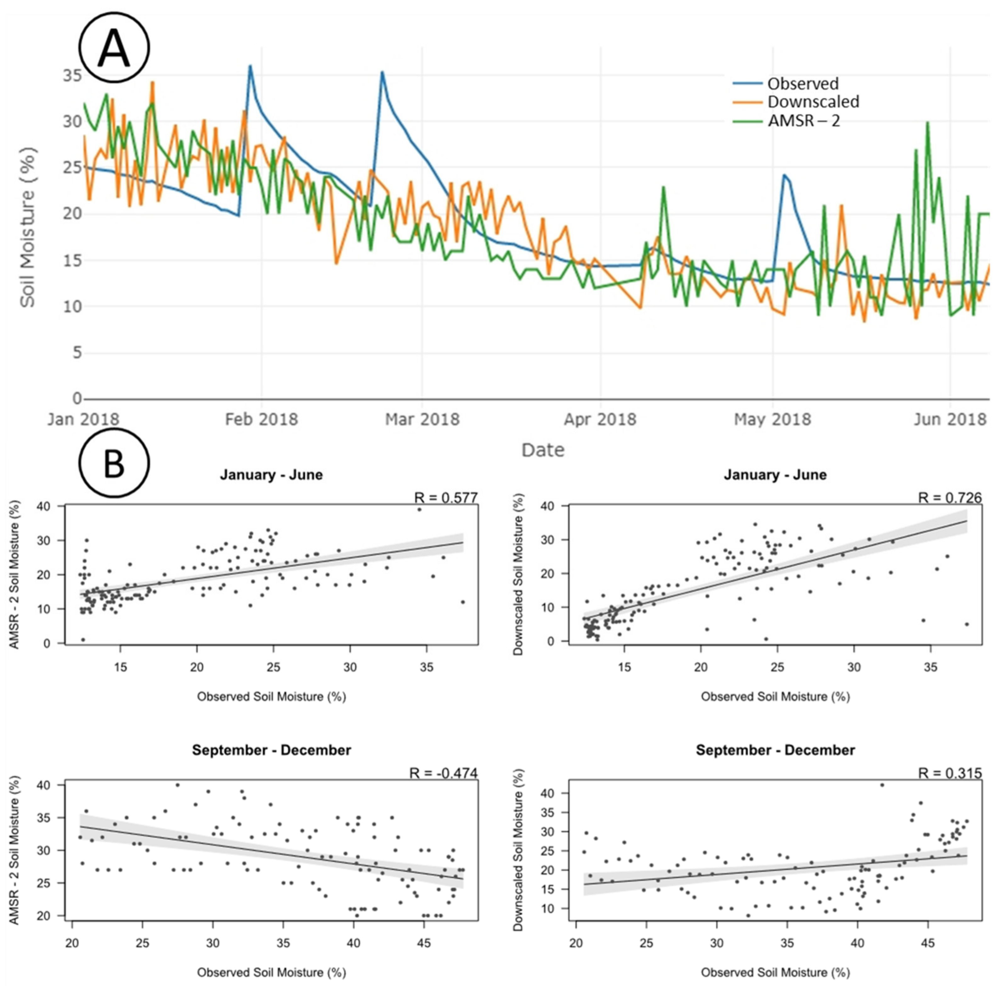
4.1. Temporal Validation of Downscaled Soil Moisture
4.2. Spatial Validation of Downscaled Soil Moisture
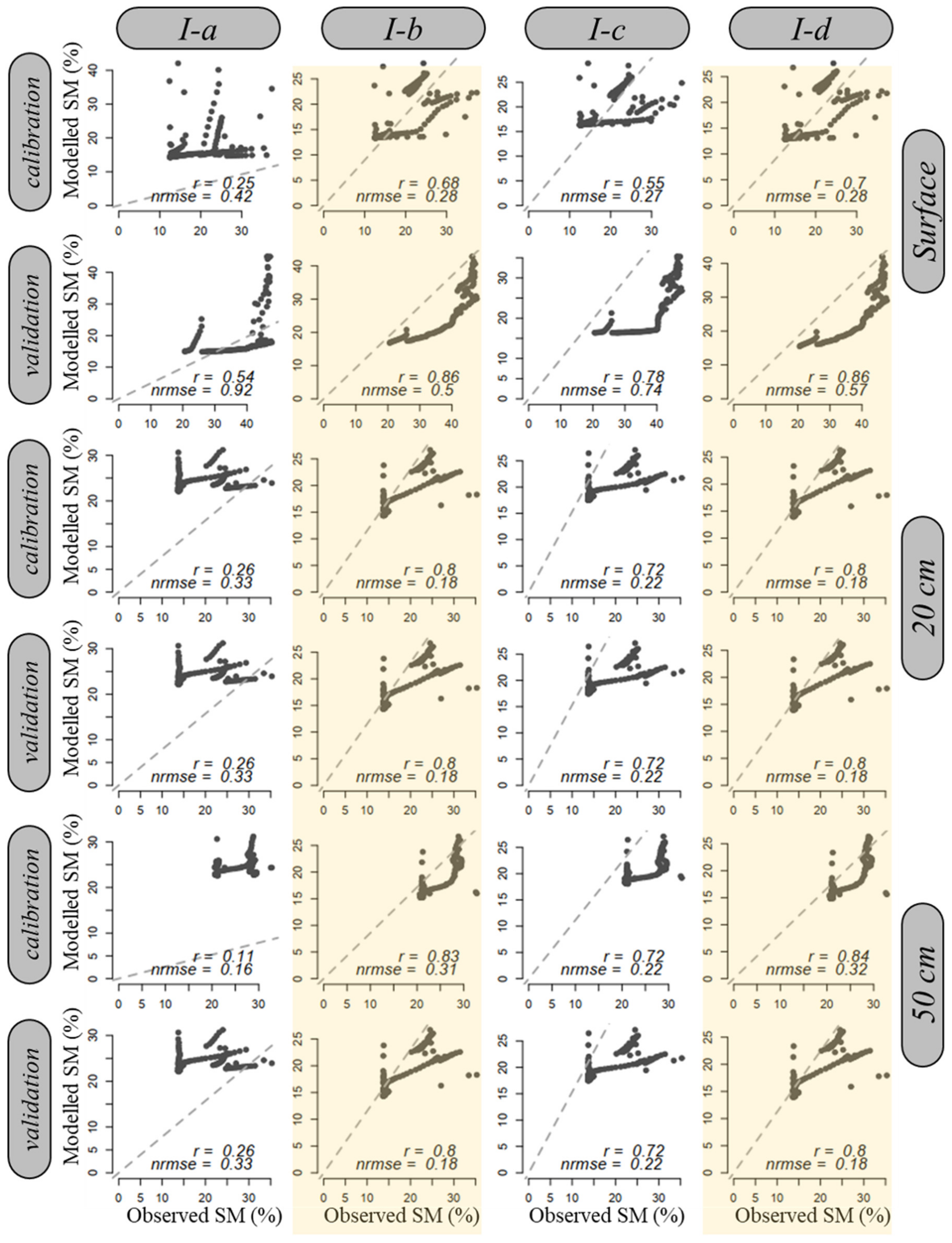
4.3. Impact on Surface Soil Moisture and RZSM Simulation Based on Estimated SHPs
4.3.1. Impact of Homogeneous Soil Profile
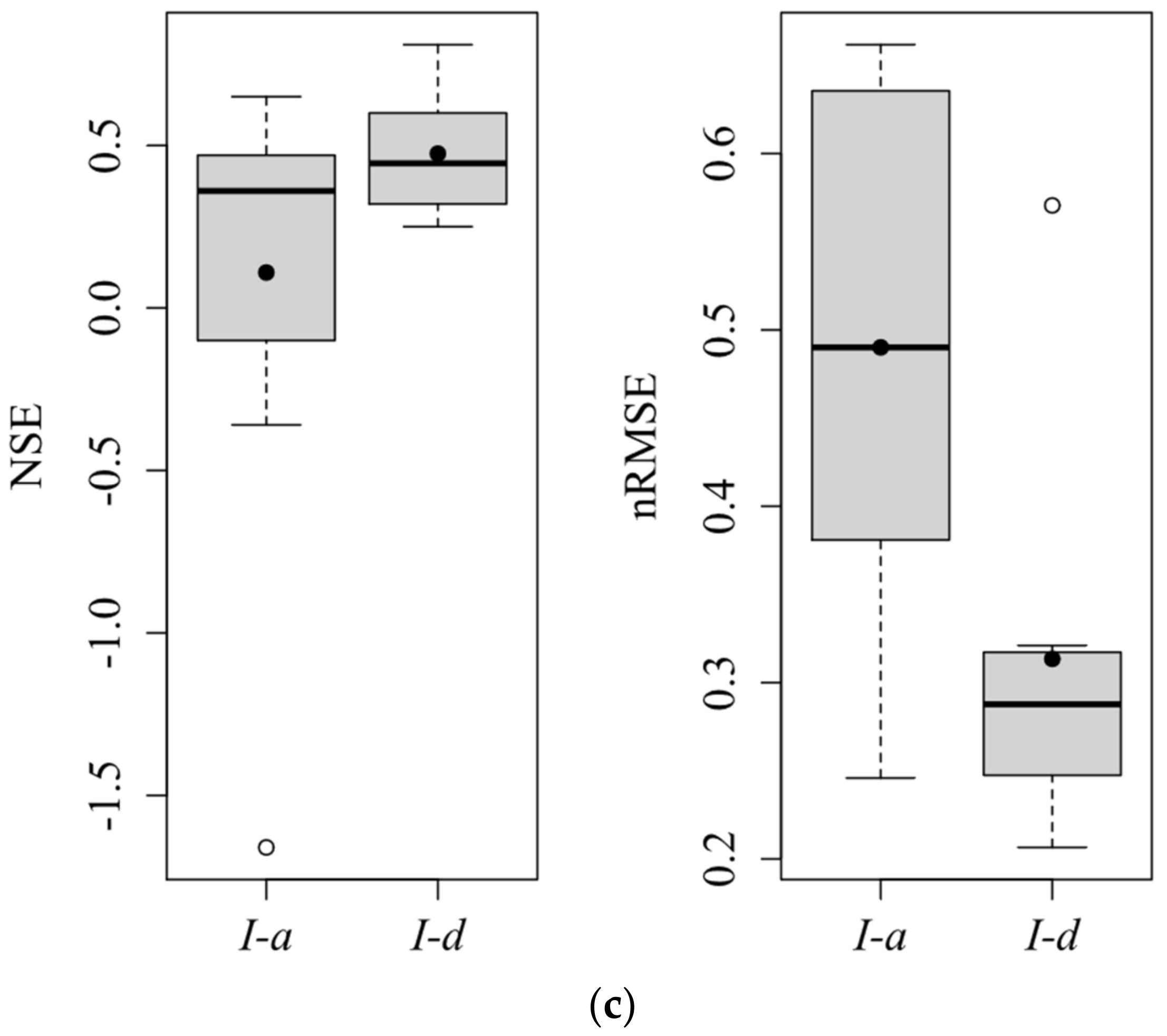
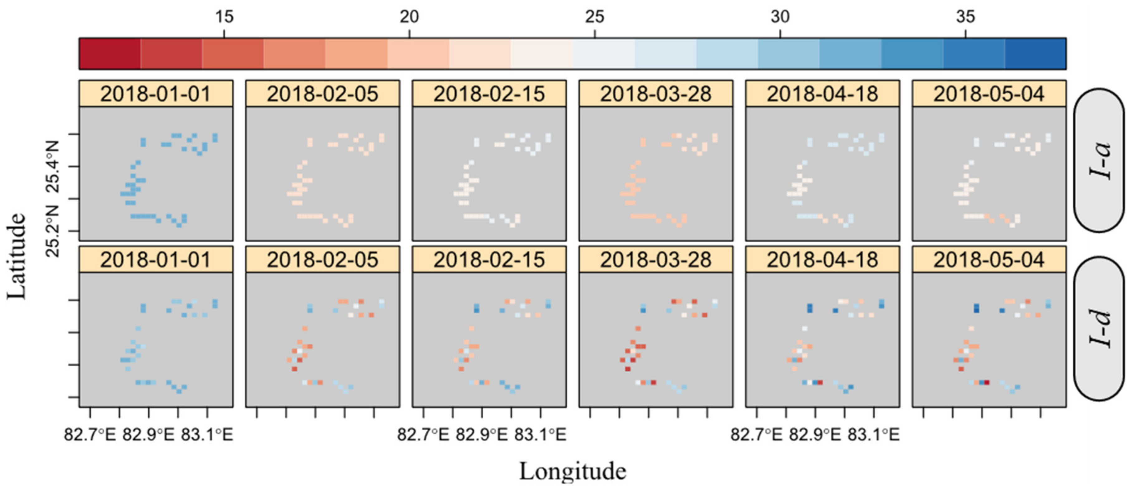
4.3.2. Impact of Heterogeneous Soil Profile
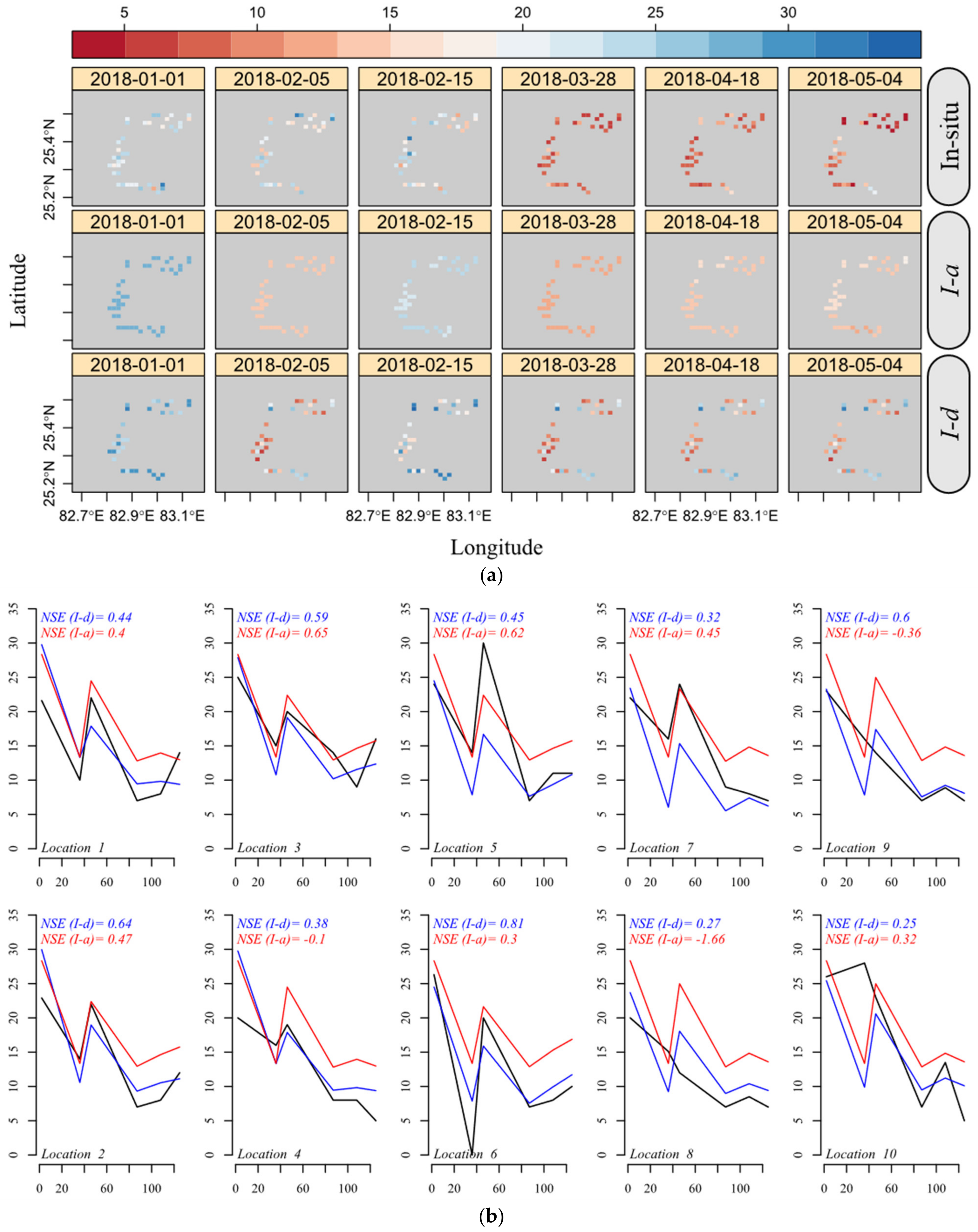
4.3.3. Rootzone Soil Moisture Geo-Product at High Temporal and Spatial Scale
5. Discussion
6. Conclusions
Author Contributions
Funding
Institutional Review Board Statement
Informed Consent Statement
Data Availability Statement
Acknowledgments
Conflicts of Interest
References
- Colliander, A.; Fisher, J.B.; Halverson, G.; Merlin, O.; Misra, S.; Bindlish, R.; Jackson, T.J.; Yueh, S. Spatial downscaling of SMAP soil moisture using MODIS land surface temperature and NDVI during SMAPVEX15. IEEE Geosci. Remote Sens. Lett. 2017, 14, 2107–2111. [Google Scholar] [CrossRef] [Green Version]
- Peng, J.; Loew, A.; Merlin, O.; Verhoest, N.E. A review of spatial downscaling of satellite remotely sensed soil moisture. Rev. Geophys. 2017, 55, 341–366. [Google Scholar] [CrossRef] [Green Version]
- Vereecken, H.; Huisman, J.; Pachepsky, Y.; Montzka, C.; Van Der Kruk, J.; Bogena, H.; Weihermüller, L.; Herbst, M.; Martinez, G.; Vanderborght, J. On the spatio-temporal dynamics of soil moisture at the field scale. J. Hydrol. 2014, 516, 76–96. [Google Scholar] [CrossRef]
- Petropoulos, G.; Carlson, T.; Wooster, M.; Islam, S. A review of Ts/VI remote sensing based methods for the retrieval of land surface energy fluxes and soil surface moisture. Prog. Phys. Geogr. 2009, 33, 224–250. [Google Scholar] [CrossRef] [Green Version]
- Bastiaanssen, W.G.; Molden, D.J.; Makin, I.W. Remote sensing for irrigated agriculture: Examples from research and possible applications. Agric. Water Manag. 2000, 46, 137–155. [Google Scholar] [CrossRef]
- Douville, H.; Viterbo, P.; Mahfouf, J.-F.; Beljaars, A.C. Evaluation of the optimum interpolation and nudging techniques for soil moisture analysis using FIFE data. Mon. Weather. Rev. 2000, 128, 1733–1756. [Google Scholar] [CrossRef]
- Nemani, R.; Hashimoto, H.; Votava, P.; Melton, F.; Wang, W.; Michaelis, A.; Mutch, L.; Milesi, C.; Hiatt, S.; White, M. Monitoring and forecasting ecosystem dynamics using the Terrestrial Observation and Prediction System (TOPS). Remote Sens. Environ. 2009, 113, 1497–1509. [Google Scholar] [CrossRef]
- Reichstein, M.; Rey, A.; Freibauer, A.; Tenhunen, J.; Valentini, R.; Banza, J.; Casals, P.; Cheng, Y.; Grünzweig, J.M.; Irvine, J. Modeling temporal and large-scale spatial variability of soil respiration from soil water availability, temperature and vegetation productivity indices. Glob. Biogeochem. Cycles 2003, 17, 1104. [Google Scholar] [CrossRef]
- Esit, M.; Kumar, S.; Pandey, A.; Lawrence, D.M.; Rangwala, I.; Yeager, S. Seasonal to multi-year soil moisture drought forecasting. NPJ Clim. Atmos. Sci. 2021, 4, 16. [Google Scholar] [CrossRef]
- Hu, W.; Xu, Q.; Wang, G.; Van Asch, T.; Hicher, P.-Y. Sensitivity of the initiation of debris flow to initial soil moisture. Landslides 2015, 12, 1139–1145. [Google Scholar] [CrossRef] [Green Version]
- Marino, P.; Peres, D.J.; Cancelliere, A.; Greco, R.; Bogaard, T.A. Soil moisture information can improve shallow landslide forecasting using the hydrometeorological threshold approach. Landslides 2020, 17, 2041–2054. [Google Scholar] [CrossRef]
- Wasko, C.; Nathan, R. Influence of changes in rainfall and soil moisture on trends in flooding. J. Hydrol. 2019, 575, 432–441. [Google Scholar] [CrossRef]
- Zeri, M.; Williams, K.; Cunha, A.P.M.; Cunha-Zeri, G.; Vianna, M.S.; Blyth, E.M.; Marthews, T.R.; Hayman, G.D.; Costa, J.M.; Marengo, J.A. Importance of including soil moisture in drought monitoring over the Brazilian semiarid region: An evaluation using the JULES model, in situ observations, and remote sensing. Clim. Resil. Sustain. 2022, 1, e7. [Google Scholar] [CrossRef]
- Zhao, Y.; Yang, H.; Wei, F. Soil moisture retrieval with remote sensing images for debris flow forecast in humid regions. Monit. Simul. Prev. Remediat. Dense Debris Flows III 2010, 67, 11189. [Google Scholar]
- Loew, A. Impact of surface heterogeneity on surface soil moisture retrievals from passive microwave data at the regional scale: The Upper Danube case. Remote Sens. Environ. 2008, 112, 231–248. [Google Scholar] [CrossRef]
- Jackson, T.J.; Hsu, A.Y.; O’Neill, P.E. Surface soil moisture retrieval and mapping using high-frequency microwave satellite observations in the Southern Great Plains. J. Hydrometeorol. 2002, 3, 688–699. [Google Scholar] [CrossRef]
- Wu, X.; Walker, J.P.; Rüdiger, C.; Panciera, R. Effect of land-cover type on the SMAP active/passive soil moisture downscaling algorithm performance. IEEE Geosci. Remote Sens. Lett. 2014, 12, 846–850. [Google Scholar]
- Wagner, W.; Naeimi, V.; Scipal, K.; de Jeu, R.; Martínez-Fernández, J. Soil moisture from operational meteorological satellites. Hydrogeol. J. 2007, 15, 121–131. [Google Scholar] [CrossRef]
- Mishra, V.; Ellenburg, W.L.; Griffin, R.E.; Mecikalski, J.R.; Cruise, J.F.; Hain, C.R.; Anderson, M.C. An initial assessment of a SMAP soil moisture disaggregation scheme using TIR surface evaporation data over the continental United States. Int. J. Appl. Earth Obs. Geoinf. 2018, 68, 92–104. [Google Scholar] [CrossRef]
- Das, N.N.; Entekhabi, D.; Dunbar, S.; Kim, S.-B.; Yueh, S.; Colliander, A.; O’Neill, P.; Jackson, T.J.; Jagdhuber, T.; Chen, F. SMAP/Sentinel-1 L2 Radiometer/Radar 30-Second Scene 3 km EASE-Grid Soil Moisture-Global; NASA National Snow and Ice Data Center Distributed Active Archive Center: Boulder, CO, USA, 2019.
- Wentz, F.; Meissner, T.; Gentemann, C.; Hilburn, K.; Scott, J. Remote Sensing Systems GCOM-W1 AMSR2 Daily Environmental Suite on 0.25 Deg Grid, version 7.2; Remote Sensing Systems: Santa Rosa, CA, USA, 2014. [Google Scholar]
- Garg, N.; Gupta, M. Assessment of improved soil hydraulic parameters for soil water content simulation and irrigation scheduling. Irrig. Sci. 2015, 33, 247–264. [Google Scholar] [CrossRef]
- Dash, S.K.; Sinha, R. A Comprehensive Evaluation of Gridded L-, C-, and X-Band Microwave Soil Moisture Product over the CZO in the Central Ganga Plains, India. Remote Sens. 2022, 14, 1629. [Google Scholar] [CrossRef]
- Merlin, O.; Al Bitar, A.; Walker, J.P.; Kerr, Y. An improved algorithm for disaggregating microwave-derived soil moisture based on red, near-infrared and thermal-infrared data. Remote Sens. Environ. 2010, 114, 2305–2316. [Google Scholar] [CrossRef] [Green Version]
- Piles, M.; Camps, A.; Vall-Llossera, M.; Corbella, I.; Panciera, R.; Rudiger, C.; Kerr, Y.H.; Walker, J. Downscaling SMOS-derived soil moisture using MODIS visible/infrared data. IEEE Trans. Geosci. Remote Sens. 2011, 49, 3156–3166. [Google Scholar] [CrossRef]
- Merlin, O.; Walker, J.P.; Chehbouni, A.; Kerr, Y. Towards deterministic downscaling of SMOS soil moisture using MODIS derived soil evaporative efficiency. Remote Sens. Environ. 2008, 112, 3935–3946. [Google Scholar] [CrossRef] [Green Version]
- Merlin, O.; Chehbouni, A.; Walker, J.P.; Panciera, R.; Kerr, Y.H. A simple method to disaggregate passive microwave-based soil moisture. IEEE Trans. Geosci. Remote Sens. 2008, 46, 786–796. [Google Scholar] [CrossRef] [Green Version]
- Merlin, O.; Al Bitar, A.; Walker, J.P.; Kerr, Y. A sequential model for disaggregating near-surface soil moisture observations using multi-resolution thermal sensors. Remote Sens. Environ. 2009, 113, 2275–2284. [Google Scholar] [CrossRef] [Green Version]
- Šimůnek, J.; van Genuchten, M.T.; Šejna, M. Development and applications of the HYDRUS and STANMOD software packages and related codes. Vadose Zone J. 2008, 7, 587–600. [Google Scholar] [CrossRef] [Green Version]
- Kottek, M.; Grieser, J.; Beck, C.; Rudolf, B.; Rubel, F. World Map of the Köppen-Geiger climate classification updated. Meteorol. Z. 2006, 15, 259–263. [Google Scholar] [CrossRef]
- Varanasi Mines Officer. District Survey Report for Planning and Execution of Minor Mineral Excavation; National Informatics Center Varanasi: Varanasi, India, 2020.
- Nistor, M.M.; Rai, P.K.; Dugesar, V.; Mishra, V.N.; Singh, P.; Arora, A.; Kumra, V.K.; Carebia, I.A. Climate change effect on water resources in Varanasi district, India. Meteorol. Appl. 2020, 27, e1863. [Google Scholar] [CrossRef] [Green Version]
- Lehner, B.; Verdin, K.; Jarvis, A. New global hydrography derived from spaceborne elevation data. EOS Trans. Am. Geophys. Union 2008, 89, 93–94. [Google Scholar] [CrossRef]
- Gruber, A.; Dorigo, W.A.; Zwieback, S.; Xaver, A.; Wagner, W. Characterizing coarse-scale representativeness of in situ soil moisture measurements from the International Soil Moisture Network. Vadose Zone J. 2013, 12, vzj2012.0170. [Google Scholar] [CrossRef] [Green Version]
- Jabro, J.; Stevens, W.; Iversen, W. Field performance of three real-time moisture sensors in sandy loam and clay loam soils. Arch. Agron. Soil Sci. 2018, 64, 930–938. [Google Scholar] [CrossRef]
- Sharma, J.; Prasad, R.; Srivastava, P.K.; Singh, S.K.; Yadav, S.A.; Yadav, V.P. Roughness characterization and disaggregation of coarse resolution SMAP soil moisture using single-channel algorithm. J. Appl. Remote Sens. 2021, 15, 014514. [Google Scholar] [CrossRef]
- Wan, Z.; Hook, S.; Hulley, G. MOD11A1 MODIS/Terra Land Surface Temperature and the Emissivity Daily L3 Global 1km SIN Grid; NASA LP DAAC: Sioux Falls, SD, USA, 2015.
- Didan, K. MOD13A2 MODIS/Terra Vegetation Indices 16-Day L3 Global 1km SIN Grid V006; NASA LP DAAC: Sioux Falls, SD, USA, 2015; No. 10.
- Myneni, R.; Knyazikhin, Y.; Park, T. MOD15A2H MODIS/Terra leaf area Index/FPAR 8-Day L4 Global 500m SIN grid V006; NASA LP DAAC: Sioux Falls, SD, USA, 2015.
- Boschetti, L.; Vermote, E.; Wolfe, R. MODTBGA MODIS/Terra Thermal Bands Daily L2G-lite Global 1km SIN grid V006; NASA LP DAAC: Sioux Falls, SD, USA, 2015.
- Owe, M.; de Jeu, R.; Walker, J. A methodology for surface soil moisture and vegetation optical depth retrieval using the microwave polarization difference index. IEEE Trans. Geosci. Remote Sens. 2001, 39, 1643–1654. [Google Scholar] [CrossRef] [Green Version]
- Dorigo, W.; Wagner, W.; Hohensinn, R.; Hahn, S.; Paulik, C.; Xaver, A.; Gruber, A.; Drusch, M.; Mecklenburg, S.; van Oevelen, P. The International Soil Moisture Network: A data hosting facility for global in situ soil moisture measurements. Hydrol. Earth Syst. Sci. 2011, 15, 1675–1698. [Google Scholar] [CrossRef] [Green Version]
- Tian, Y.; Peters-Lidard, C.D.; Kumar, S.V.; Geiger, J.; Houser, P.R.; Eastman, J.L.; Dirmeyer, P.; Doty, B.; Adams, J. High-performance land surface modeling with a Linux cluster. Comput. Geosci. 2008, 34, 1492–1504. [Google Scholar] [CrossRef]
- Stackhouse, P.; Zhang, T.; Westberg, D.; Barnett, A.J.; Bristow, T.; Macpherson, B.; Hoell, J.M. POWER Release 8.0. 1 (with GIS applications) Methodology (Data Parameters, Sources, & Validation); NASA Langley Research Centre: Hampton, VA, USA, 2018.
- Li, Z.-L.; Tang, R.; Wan, Z.; Bi, Y.; Zhou, C.; Tang, B.; Yan, G.; Zhang, X. A review of current methodologies for regional evapotranspiration estimation from remotely sensed data. Sensors 2009, 9, 3801–3853. [Google Scholar] [CrossRef] [Green Version]
- Goetz, S. Multi-sensor analysis of NDVI, surface temperature and biophysical variables at a mixed grassland site. Int. J. Remote Sens. 1997, 18, 71–94. [Google Scholar] [CrossRef]
- Nemani, R.; Pierce, L.; Running, S.; Goward, S. Developing satellite-derived estimates of surface moisture status. J. Appl. Meteorol. Climatol. 1993, 32, 548–557. [Google Scholar] [CrossRef]
- Rahimzadeh-Bajgiran, P.; Berg, A. Soil moisture retrievals using optical/TIR methods. In Satellite Soil Moisture Retrieval; Elsevier: Amsterdam, The Netherlands, 2016; pp. 47–72. [Google Scholar]
- Team, R.C. R: A Language and Environment for Statistical Computing; RC Team: Vienna, Austria, 2013. [Google Scholar]
- Mattiuzzi, M.; Detsch, F. MODIS: Acquisition and Processing of MODIS Products; RC Team: Vienna, Austria, 2016. [Google Scholar]
- Atzberger, C.; Eilers, P.H. A time series for monitoring vegetation activity and phenology at 10-daily time steps covering large parts of South America. Int. J. Digit. Earth 2011, 4, 365–386. [Google Scholar] [CrossRef]
- Pablos, M.; González-Zamora, Á.; Sánchez, N.; Martínez-Fernández, J. Assessment of root zone soil moisture estimations from SMAP, SMOS and MODIS observations. Remote Sens. 2018, 10, 981. [Google Scholar] [CrossRef] [Green Version]
- Gupta, M.; Garg, N.; Joshi, H.; Sharma, M. Persistence and mobility of 2, 4-D in unsaturated soil zone under winter wheat crop in sub-tropical region of India. Agric. Ecosyst. Environ. 2012, 146, 60–72. [Google Scholar] [CrossRef]
- Allen, R.G.; Pereira, L.S.; Raes, D.; Smith, M. Crop Evapotranspiration-Guidelines for Computing Crop Water Requirements; FAO Irrigation and Drainage Paper 56; FAO: Rome, Italy, 1998; Volume 300, p. D05109. [Google Scholar]
- Van Genuchten, M.T. A closed-form equation for predicting the hydraulic conductivity of unsaturated soils. Soil Sci. Soc. Am. J. 1980, 44, 892–898. [Google Scholar] [CrossRef] [Green Version]
- Mualem, Y. A new model for predicting the hydraulic conductivity of unsaturated porous media. Water Resour. Res. 1976, 12, 513–522. [Google Scholar] [CrossRef] [Green Version]
- Srivastava, P.K.; Petropoulos, G.P.; Prasad, R.; Triantakonstantis, D. Random Forests with Bagging and Genetic Algorithms Coupled with Least Trimmed Squares Regression for Soil Moisture Deficit Using SMOS Satellite Soil Moisture. ISPRS Int. J. Geo-Inf. 2021, 10, 507. [Google Scholar] [CrossRef]
- Srivastava, P.K.; Han, D.; Yaduvanshi, A.; Petropoulos, G.P.; Singh, S.K.; Mall, R.K.; Prasad, R. Reference evapotranspiration retrievals from a mesoscale model based weather variables for soil moisture deficit estimation. Sustainability 2017, 9, 1971. [Google Scholar] [CrossRef] [Green Version]


| SHPs | Ks | θs | θr | α | n |
|---|---|---|---|---|---|
| Lower Limit | 15 | 0.35 | 0.01 | 0.0007 | 1 |
| Upper Limit | 35 | 0.43 | 0.07 | 0.1 | 2 |
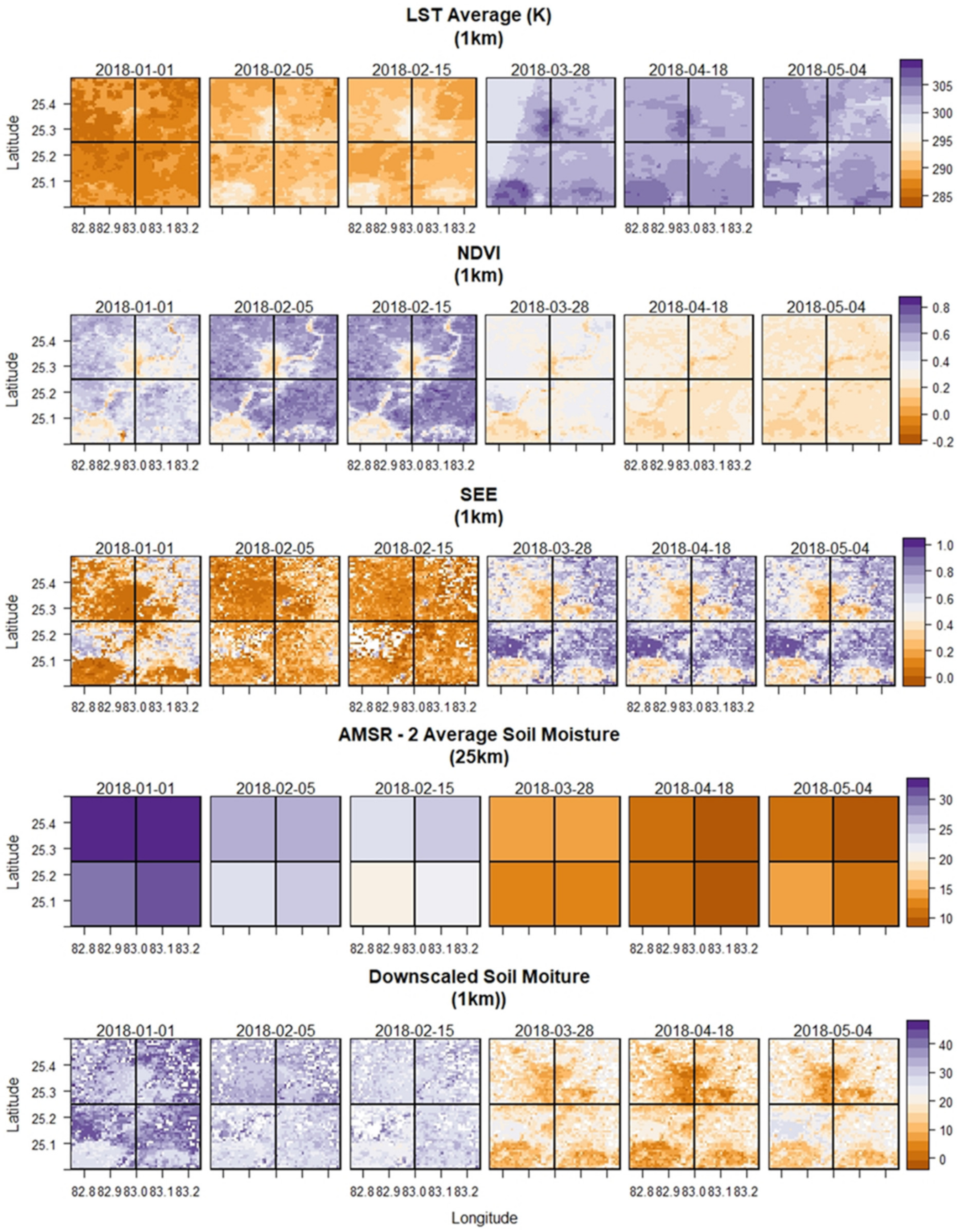
| Variables | 1 January 2018 | 5 February 2018 | 16 February 2018 | 28 March 2018 | 18 April 2018 | 4 May 2018 |
|---|---|---|---|---|---|---|
| LST | 286–288 * (287.11) | 289.82–291.62 (290.60) | 289.98–291.66 (291.07) | 300.71–302.65 (301.53) | 302.45–303.47 (302.80) | 301.84–303.64 (302.86) |
| NDVI | 0.48–0.66 (0.44) | 0.28–0.35 (0.60) | 0.48–0.66 (0.61) | 0.28–0.35 (0.32) | 0.22–0.26 (0.24) | 0.20–0.24 (0.22) |
| SEE | 0.07–0.49 (0.28) | 0.09–0.25 (0.16) | 0.07–0.19 (0.12) | 0.44–0.75 (0.60) | 0.46–0.76 (0.61) | 0.45–0.75 (0.60) |
| AMSR-2 SM | 30.75–32.00 (31.50) | 24.75–26.25 (25.50) | 21.75–23.75 (22.75) | 13.00–13.50 (13.25) | 10.00–11.00 (10.50) | 10.75–11.75 (11.00) |
| Downscaled SM | 28.97–39.16 (34.25) | 27.51–32.78 (30.34) | 25.99–29.85 (27.68) | 12.35–20.06 (16.43) | 9.35–17.29 (13.68) | 13.00–21.00 (17.58) |
| Soil Profile | Experiment No. | Soil Depth (cm) | Soil Hydraulic Parameters | Soil Depth (cm) | Calibration | Validation | ||||||
|---|---|---|---|---|---|---|---|---|---|---|---|---|
| Ks | θs | θr | α | n | Cor | nRMSE | Cor | nRMSE | ||||
| Homogeneous | I-a | 0–100 | 10.80 | 0.45 | 0.07 | 0.0200 | 1.41 | 0–15 | 0.49 | 0.38 | 0.78 | 0.50 |
| 15–30 | 0.32 | 0.43 | 0.92 | 0.22 | ||||||||
| 30–100 | 0.09 | 0.16 | 0.98 | 0.18 | ||||||||
| I-b | 0–100 | 31.66 | 0.43 | 0.03 | 0.0008 | 1.31 | 0–15 | 0.76 | 0.25 | 0.96 | 0.34 | |
| 15–30 | 0.70 | 0.19 | 0.91 | 0.28 | ||||||||
| 30–100 | 0.81 | 0.24 | 0.98 | 0.31 | ||||||||
| I-c | 0–100 | 20.67 | 0.35 | 0.07 | 0.0011 | 1.24 | 0–15 | 0.73 | 0.27 | 0.91 | 0.43 | |
| 15–30 | 0.67 | 0.25 | 0.9 | 0.35 | ||||||||
| 30–100 | 0.78 | 0.18 | 0.98 | 0.37 | ||||||||
| I-d | 0–100 | 32.54 | 0.42 | 0.04 | 0.0009 | 1.33 | 0–15 | 0.76 | 0.25 | 0.96 | 0.37 | |
| 15–30 | 0.71 | 0.18 | 0.91 | 0.31 | ||||||||
| 30–100 | 0.82 | 0.25 | 0.98 | 0.34 | ||||||||
| Heterogeneous | II-a | 0–15 | 10.80 | 0.45 | 0.07 | 0.0200 | 1.41 | 0–15 | 0.45 | 0.39 | 0.81 | 0.48 |
| 15–30 | 10.80 | 0.45 | 0.07 | 0.0200 | 1.41 | 15–30 | 0.19 | 0.37 | 0.92 | 0.22 | ||
| 30–100 | 1.68 | 0.43 | 0.09 | 0.0100 | 1.23 | 30–100 | −0.35 | 0.29 | 0.98 | 0.1 | ||
| II-b | 0–15 | 16.57 | 0.36 | 0.01 | 0.0500 | 1.163 | 0–15 | 0.73 | 0.27 | 0.87 | 0.43 | |
| 15–30 | 22.81 | 0.39 | 0.07 | 0.0600 | 1.05 | 15–30 | 0.68 | 0.39 | 0.91 | 0.55 | ||
| 30–100 | 24.86 | 0.43 | 0.02 | 0.0240 | 1.324 | 30–100 | 0.53 | 0.42 | 0.98 | 0.48 | ||
| Station | Ks | θs | θr | α | n | Station | Ks | θs | θr | α | n |
|---|---|---|---|---|---|---|---|---|---|---|---|
| HDS-01 | 18.47 | 0.41 | 0.01 | 0.047 | 1.15 | HDS-23 | 34.97 | 0.38 | 0.07 | 0.022 | 1.14 |
| HDS-02 | 21.95 | 0.37 | 0.04 | 0.046 | 1.35 | HDS-24 | 29.78 | 0.40 | 0.05 | 0.018 | 1.29 |
| HDS-03 | 21.98 | 0.42 | 0.05 | 0.005 | 1.60 | HDS-25 | 22.05 | 0.37 | 0.06 | 0.042 | 1.78 |
| HDS-04 | 17.11 | 0.42 | 0.06 | 0.024 | 1.04 | HDS-26 | 24.62 | 0.37 | 0.07 | 0.052 | 1.08 |
| HDS-05 | 17.11 | 0.42 | 0.06 | 0.024 | 1.04 | HDS-27 | 23.75 | 0.40 | 0.03 | 0.062 | 1.65 |
| HDS-06 | 24.65 | 0.39 | 0.06 | 0.017 | 1.59 | HDS-28 | 17.53 | 0.38 | 0.02 | 0.042 | 1.80 |
| HDS-07 | 24.54 | 0.43 | 0.05 | 0.085 | 1.86 | HDS-29 | 15.55 | 0.42 | 0.06 | 0.039 | 1.83 |
| HDS-08 | 17.11 | 0.42 | 0.06 | 0.024 | 1.04 | HDS-30 | 29.78 | 0.40 | 0.05 | 0.018 | 1.29 |
| HDS-09 | 23.65 | 0.39 | 0.07 | 0.002 | 1.73 | HDS-31 | 23.23 | 0.38 | 0.05 | 0.002 | 1.10 |
| HDS-10 | 21.98 | 0.42 | 0.05 | 0.005 | 1.60 | HDS-32 | 33.71 | 0.40 | 0.05 | 0.008 | 1.14 |
| HDS-11 | 22.05 | 0.37 | 0.06 | 0.042 | 1.78 | HDS-33 | 32.18 | 0.39 | 0.01 | 0.006 | 1.14 |
| HDS-12 | 17.53 | 0.38 | 0.02 | 0.042 | 1.80 | HDS-34 | 23.73 | 0.41 | 0.05 | 0.005 | 1.18 |
| HDS-13 | 29.78 | 0.40 | 0.05 | 0.018 | 1.29 | HDS-35 | 22.68 | 0.38 | 0.02 | 0.008 | 1.08 |
| HDS-14 | 21.95 | 0.37 | 0.04 | 0.008 | 1.04 | HDS-36 | 22.34 | 0.39 | 0.07 | 0.008 | 1.11 |
| HDS-15 | 34.43 | 0.41 | 0.04 | 0.085 | 1.00 | HDS-37 | 28.52 | 0.42 | 0.03 | 0.010 | 1.07 |
| HDS-16 | 23.75 | 0.40 | 0.03 | 0.062 | 1.65 | HDS-38 | 22.68 | 0.38 | 0.02 | 0.008 | 1.08 |
| HDS-17 | 24.11 | 0.36 | 0.02 | 0.023 | 1.04 | HDS-39 | 21.5 | 0.43 | 0.05 | 0.015 | 1.06 |
| HDS-18 | 20.57 | 0.42 | 0.04 | 0.079 | 1.84 | HDS-40 | 27.65 | 0.37 | 0.02 | 0.095 | 1.46 |
| HDS-19 | 24.52 | 0.42 | 0.05 | 0.064 | 1.74 | HDS-41 | 22.26 | 0.39 | 0.07 | 0.049 | 1.38 |
| HDS-20 | 34.29 | 0.37 | 0.04 | 0.057 | 1.46 | HDS-42 | 18.1 | 0.36 | 0.01 | 0.012 | 1.10 |
| HDS-21 | 24.11 | 0.36 | 0.02 | 0.023 | 1.04 | HDS-43 | 21.09 | 0.39 | 0.04 | 0.006 | 1.12 |
| HDS-22 | 34.29 | 0.37 | 0.04 | 0.057 | 1.46 | HDS-44 | 18.39 | 0.36 | 0.04 | 0.007 | 1.10 |
Disclaimer/Publisher’s Note: The statements, opinions and data contained in all publications are solely those of the individual author(s) and contributor(s) and not of MDPI and/or the editor(s). MDPI and/or the editor(s) disclaim responsibility for any injury to people or property resulting from any ideas, methods, instructions or products referred to in the content. |
© 2023 by the authors. Licensee MDPI, Basel, Switzerland. This article is an open access article distributed under the terms and conditions of the Creative Commons Attribution (CC BY) license (https://creativecommons.org/licenses/by/4.0/).
Share and Cite
Thomas, J.; Gupta, M.; Srivastava, P.K.; Pandey, D.K.; Bindlish, R. Development of High-Resolution Soil Hydraulic Parameters with Use of Earth Observations for Enhancing Root Zone Soil Moisture Product. Remote Sens. 2023, 15, 706. https://doi.org/10.3390/rs15030706
Thomas J, Gupta M, Srivastava PK, Pandey DK, Bindlish R. Development of High-Resolution Soil Hydraulic Parameters with Use of Earth Observations for Enhancing Root Zone Soil Moisture Product. Remote Sensing. 2023; 15(3):706. https://doi.org/10.3390/rs15030706
Chicago/Turabian StyleThomas, Juby, Manika Gupta, Prashant K. Srivastava, Dharmendra K. Pandey, and Rajat Bindlish. 2023. "Development of High-Resolution Soil Hydraulic Parameters with Use of Earth Observations for Enhancing Root Zone Soil Moisture Product" Remote Sensing 15, no. 3: 706. https://doi.org/10.3390/rs15030706