1. Introduction
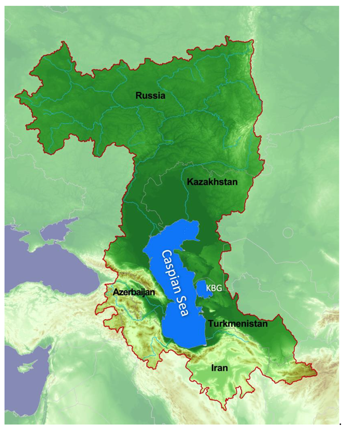
The Caspian Sea is the largest lake on Earth with an area of about 371,000 km
2. Over the past few hundred years, the Caspian Sea level (CSL) has experienced substantial fluctuations up to several meters [
1,
2,
3]. The Caspian Sea is located within an endorheic basin between Europe and Asia, and the CSL change is mainly controlled by water mass exchange between the Caspian Sea and Caspian drainage basin (see
Figure 1) via river discharge, precipitation, and evaporation. Over the past three decades, the CSL shows a large and steady decreasing trend on top of strong seasonal fluctuations, which is believed to be driven by imbalanced water fluxes or increased evaporation over the Caspian Sea due to global warming [
3,
4,
5]. The CSL is projected to fall by 9–18 m by the end of this century under the medium to high emissions scenarios [
6], which is expected to cause catastrophic impacts on the Caspian Sea coastal regions, especially in the northern part where most of the water depths are less than only 5–10 m [
5]. If this were to happen, the Kara-Bogaz-Gol (KBG) Bay would dry up completely.
Accurate measurements of CSL change play a critical role in understanding CSL variability at different temporal scales and connections with driving forces in the global and regional climate system and predicting future CSL change and potential impacts on the ecosystem in the Caspian Sea region. Tide gauge observations are also important for monitoring CSL change, especially at long-term time scales (from multi-decadal to a hundred years). However, due to special data policies in the surrounding countries, most (if not all) tide gauge observations along the Caspian Sea coasts are not available to the general public. Other challenges in using and interpreting tide gauge observations include the inconsistent temporal coverages, data qualities, and vertical land movements of the tide gauge stations.
Satellite remote sensing has become an advanced observational tool to monitor the global ocean since the late 70s. Satellite-borne Synthetic Aperture Radar technique has been used since 1978 for sea surface monitoring, as well as for mapping applications [
7,
8,
9]. Satellite radar altimeter experiments were also started at about the same time, with the accuracies of the early altimeter sea level observations at only meter level, inadequate for meaningful sea level change studies.
Since the launch of the TOPEX/Poseidon (T/P) high-accuracy satellite radar altimeter mission in August 1992, modern satellite altimeters have provided continuous measurements of global sea level (including large lakes water level) changes with unprecedented accuracy for over 30 years [
10,
11]. Altimeter-observed global sea level changes are commonly presented as global gridded sea level anomalies (SLA), defined as residual sea level changes after effects from ocean tides and atmospheric loading have been removed [
12,
13]. Estimating large lake water level change from a satellite altimeter involves some additional challenges due to the small spatial scales and different dynamical processes compared to the ocean [
14]. Specially calibrated water level changes for over hundreds of large lakes in the world are available from the Hydroweb project (
http://hydroweb.theia-land.fr/; accessed on 24 October 2022) developed by LEGOS (Laboratoire d’Etudes en Géophysique et Océanographie Spatiales) and CNES (Centre National d’Etudes Spatiales) [
14,
15].
In the present study, we carry out an analysis of CSL variations over the period of January 1993 to December 2021 using multi-satellite altimeter measurements. Two monthly CSL change series are included in the analysis. One is the specially calibrated CSL change series provided by the Hydroweb project and the other is estimated from the global SLA grids distributed by the Copernicus Marine Environment Monitoring Service (CMEMS,
https://marine.copernicus.eu/; accessed on 27 July 2022). The main goals are to (1) study CSL variations at different time scales during the past 30 years; (2) compare CSL changes from the two data sources; and (3) investigate potential discrepancies between the two altimeter-based CSL estimates and identify the causes for the discrepancies.
2. Altimeter Observed CSL Changes
The Hydroweb project has been providing satellite altimeter-observed water level time series of selected major lakes in the world in near real-time via an automated algorithm by combing observations from multi-satellites altimeter missions, including T/P, Jason-1, -2, and -3 series, Geosat Follow-On, Envisat, and others [
14,
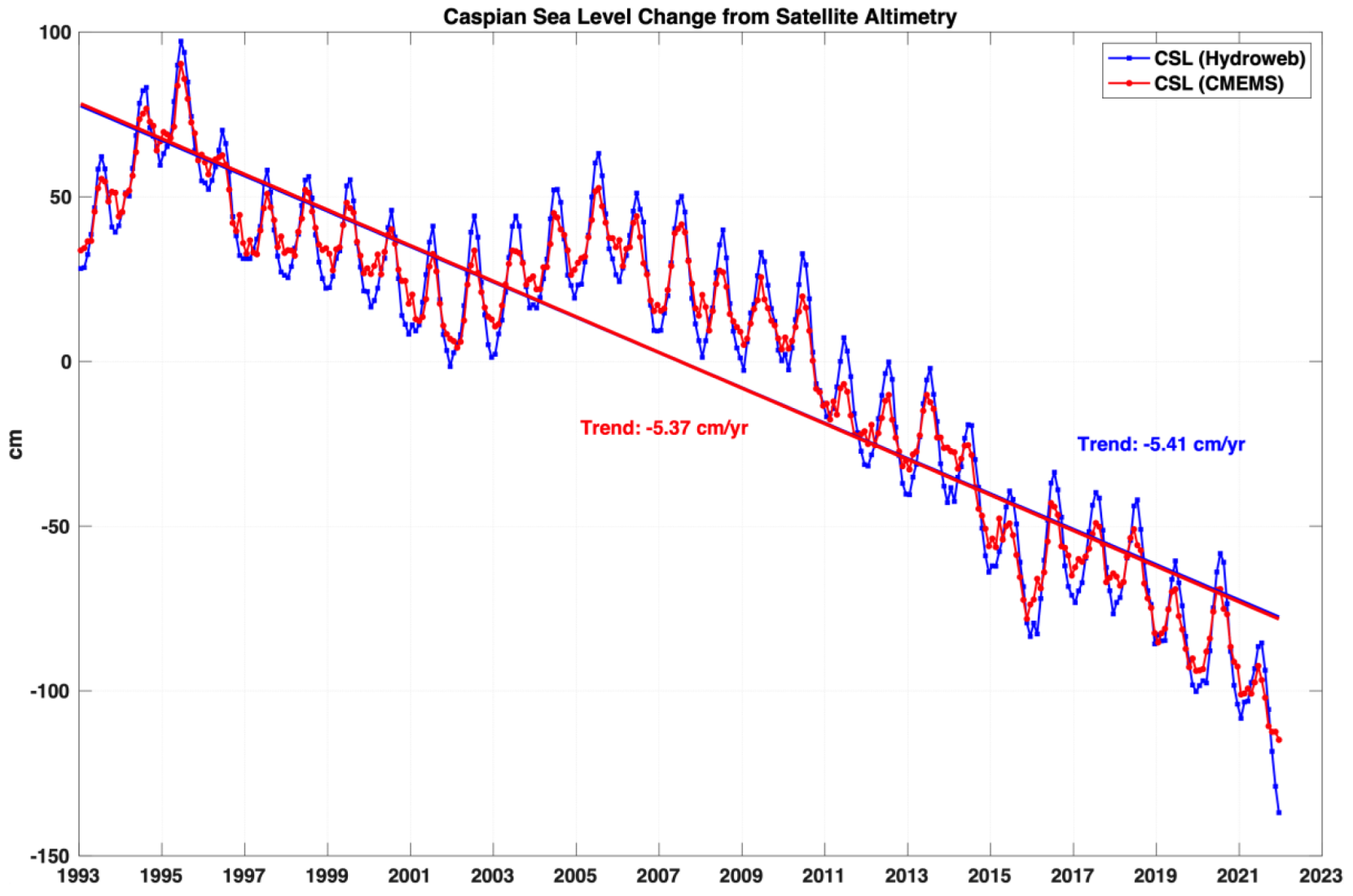
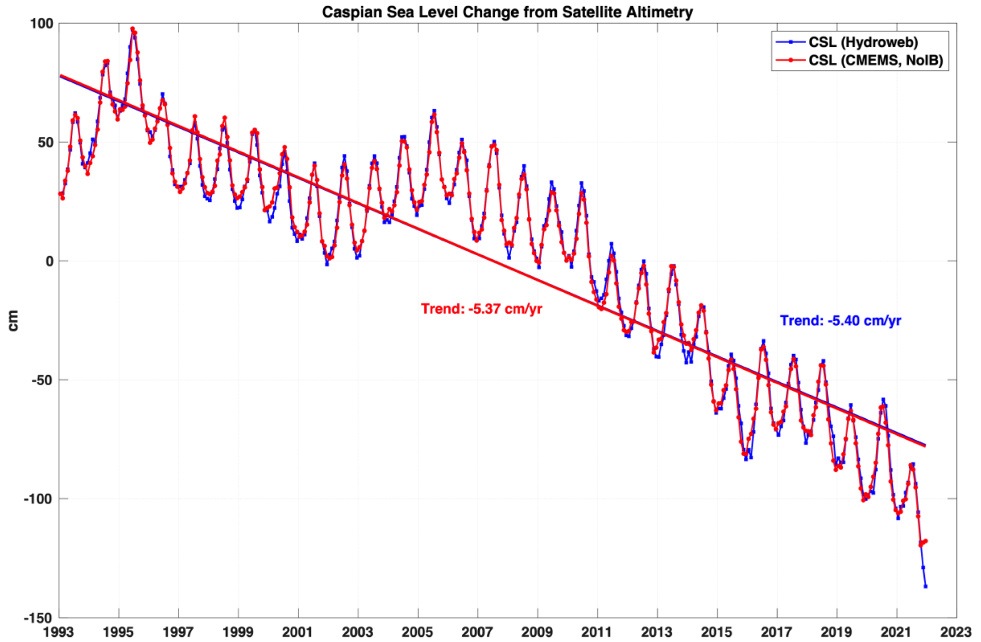
15]. The original Hydroweb CSL series is irregularly sampled (with intervals from ~10 days in early years to less than a day in recent years). The Hydroweb CSL series has been resampled to monthly intervals by taking the mean of all estimates for a given month. Water level variations for the Caspian Sea and KBG are separately provided from Hydroweb. KBG is connected to the Caspian Sea via a narrow channel, and KBG shows similar but notably different variabilities compared to the Caspian Sea. In the present analysis, we focus on the Caspian Sea, with KBG only included in the inverted barometer (IB) related analysis. The monthly Hydroweb CSL series over the period of January 1993 to December 2021 is shown in
Figure 2 (blue curves).
Global monthly mean SLA estimates given on 0.25° × 0.25° grids and covering the period January 1993 to December 2021 are provided by CMEMS. The CSL anomaly estimates are also included in the CMEMS SLA grids. The CMEMS global SLA grids are also derived from multi-satellite altimeter missions (similar to the Hydroweb lake level data). Monthly CMEMS CSL changes are computed from the CMEMS SLA grids over the Caspian Sea with the cosine of latitude as weighting. To be consistent with the Hydroweb CSL series, KBG is also excluded in the CMEMS CSL computation. As mentioned above, effects from ocean tides and atmospheric loading (i.e., IB -Inverted Barometer-) have been removed from the CMEMS SLA grids. Since the Caspian Sea is an enclosed water body, in theory, the ocean tide and IB corrections should not affect the estimated mean CSL change. The CMEMS monthly CSL change series (red curves) is compared with the Hydroweb estimates (blue curves) in
Figure 2.
Annual and semiannual amplitudes and phases and linear trends from the two-altimeter CSL estimates are estimated from least-squares fit using the following equation,
In which, and represent the altimeter monthly CSL series and time epochs; and represent the annual and semiannual amplitudes; and and represent the annual and semiannual phases. represents the linear trend and b is the mean.
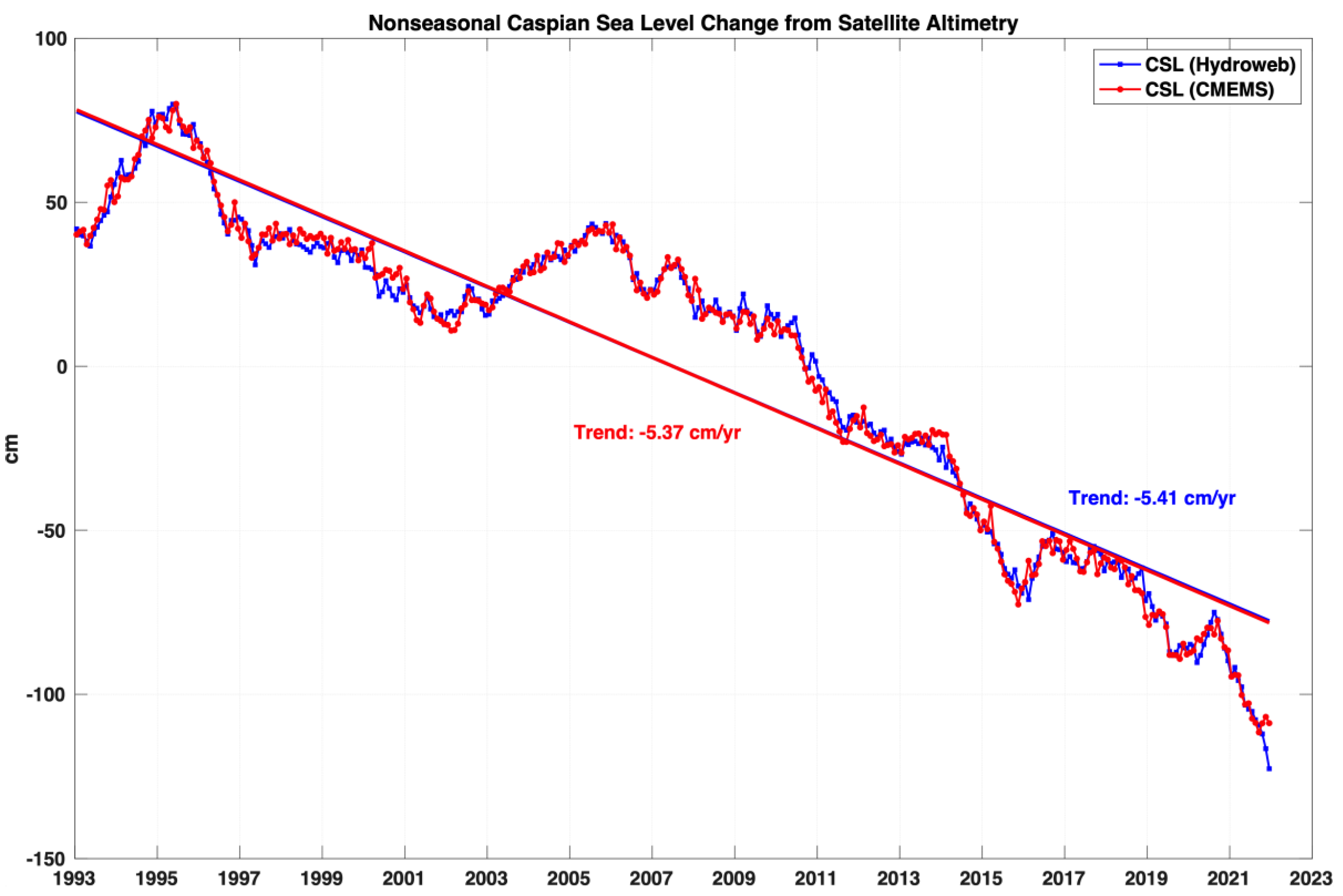
Both CSL change series exhibit similar decreasing trends and other long-term variabilities over the 30-year period, with the trends appearing to accelerate since around 2005. However, the CMEMS CSL series show significantly smaller seasonal variability, as compared to the Hydroweb estimates. To better understand the discrepancy, we estimate annual and semiannual variations using least-squares fit and remove them from both CSL series and compare the two nonseasonal CSL series in
Figure 3. It becomes more obvious—the two altimeter CSL series agree remarkably well at interannual time scales. In another word, it confirms that the discrepancy is mostly at seasonal time scales. The estimated linear trends for the Hydroweb and CMEMS CSL series are −5.37 ± 0.11 and −5.40 ± 0.11 cm/yr, respectively (virtually the same). However, the estimated mean annual amplitude of the Hydroweb CSL series is 17.03 ± 1.33 cm, which is twice as large as that (8.72 ± 1.30 cm) from the CMEMS CSL series, although the annual phases are nearly the same (266 ± 4 vs. 265 ± 9 degree).
Table 1 summarizes the comparisons of annual and semiannual amplitudes and phases and linear trends from the two-altimeter CSL estimates (see rows 1–2).
3. Atmospheric Loading Effects on CSL Change
Given the particularly large magnitude (8–9 cm) and frequency band (seasonal) of the discrepancy between the two altimeter CSL change estimates, one likely cause may be the inconsistent treatments of atmospheric loading effects on CSL change through the IB correction. In the CMEMS altimeter global SLA grids, sea level change due to atmospheric loading is removed using the IB assumption, by adjusting the sea level to changes in barometric pressure as [
16,
17],
in which,
is the IB correction to sea level in units of cm,
is sea surface pressure in units of mb (mBar) at a given grid point, and
(in mb) is the global mean sea surface pressure over the oceans, also called reference mean pressure. In the case of full adjustment, an increase in barometric pressure of 1 mb corresponds to a fall in sea level of ~1 cm. In the IB correction, this pressure-driven sea level change needs to be removed from altimeter observations [
12].
Equation (2) shows that the integration of IB effects over the global ocean is zero, which means the IB effect only changes the spatial viability of the sea (or water) level, but not the global mean sea level change (or mean CSL change). The same IB Equation (2) can be applied to large lakes as well (for small lakes, the IB effect is negligible). However, for large lakes, the IB correction needs to be implemented separately, i.e., treating each enclosed lake as an individual ocean surface. The reference mean pressure
needs to be defined as the mean surface pressure over the specific lake (e.g., Caspian Sea) as
In the Hydroweb altimeter lake-level data processing, the IB effect is not considered [
14]. Considering IB or not will give the same result, as the derived mean lake level change is not affected by the IB effect. This means that if the IB correction was implemented correctly in the CMEMS SLA grids, the atmospheric loading effect should not be responsible for the observed discrepancy between the Hydroweb and CMEMS CSL series.
Upon the clarifications from the CMEMS Sea Level Thematic Center (Françoise Mertz, Mercator-Ocean, personal communications), during the CMEMS SLA data processing, an approximate IB correction was applied for the Caspian Sea, in which the reference mean pressure used was the same as for the ocean, i.e., global mean sea level pressure over the ocean (). The difference between the approximate reference mean pressure () and the actual reference mean pressure () is expected to lead to a significant difference in the IB corrections and thus SLA estimates.
4. Improved Quantification of IB Effects on CSL Change
To better understand the potential impacts of the approximate IB correction on CMEMS CSL estimates, we use the global mean sea level pressure fields from the European Centre for Medium-Range Weather Forecasts (ECMWF) ERA5 reanalysis [
18] to quantify the CMEMS approximate and actual IB effects on Caspian Sea SLA and CSL change. ERA5 is the latest generation (5th) of the ECMWF reanalysis system developed through the Copernicus Climate Change Service [
19]. The ERA5 monthly mean sea level pressure fields on 0.25° × 0.25° grids over the period January 1993 to December 2021 are provided by the Copernicus Climate Data Store (
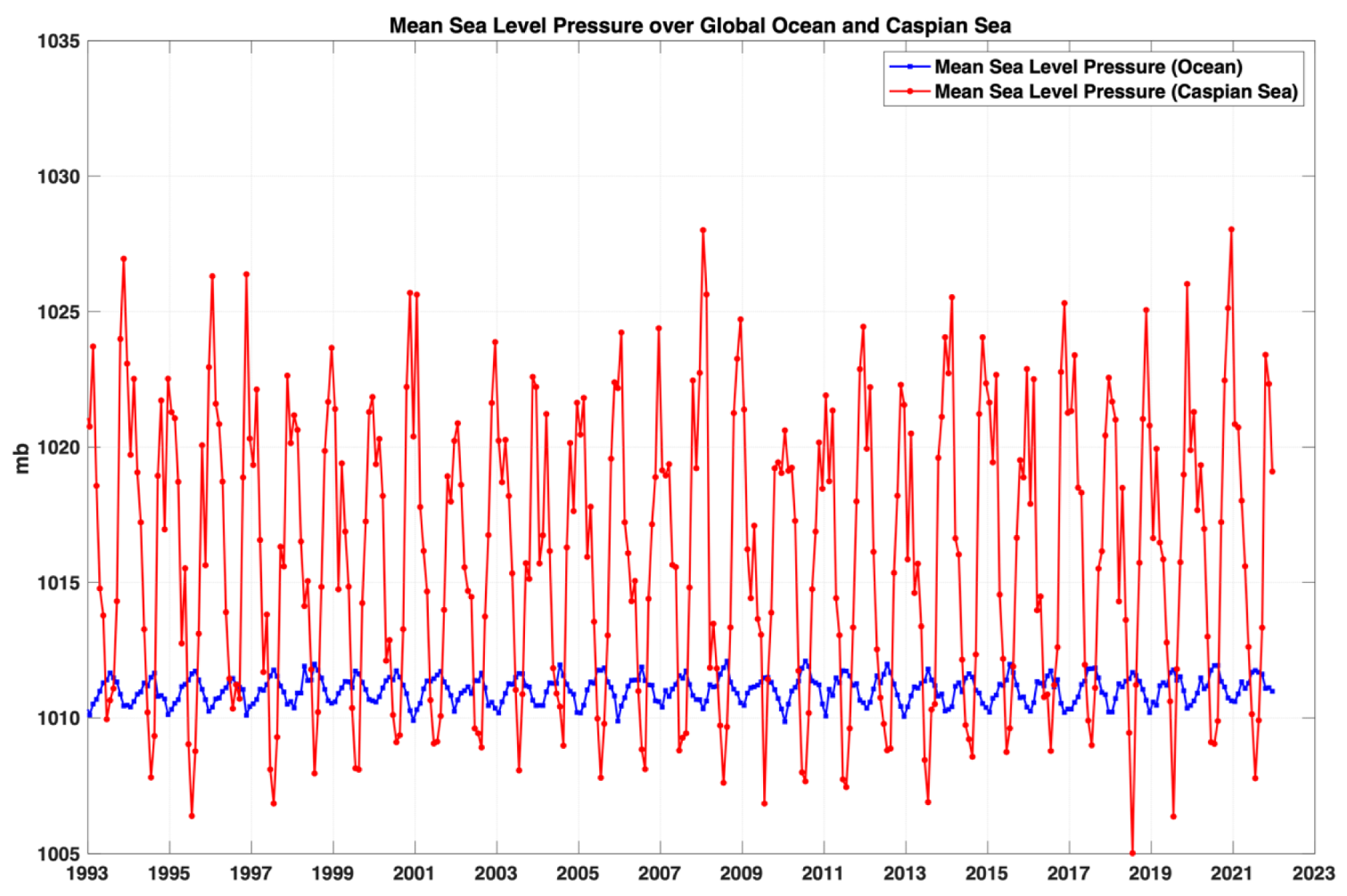
https://cds.climate.copernicus.eu/; accessed on 24 November 2022). Monthly mean sea level pressure changes over the global ocean and the Caspian Sea are computed from the ERA5 sea level pressure fields and compared in
Figure 4. Not surprisingly, the two mean sea level pressure series or the two reference mean pressure series (
and
) for the IB correction differ substantially. The seasonal variability of the global mean sea level pressure over the ocean is much smaller than that over the Caspian Sea. The large differences (up to over 10 mb) in the two mean sea level pressure series will be translated into up to over 10 cm differences in the derived SLA.
For each grid point over the Caspian Sea, the actual and CMEMS approximate IB corrections are computed from the ERA5 sea level data using
and
as the reference mean pressure, respectively. Annual amplitudes at each grid point from the two IB corrections are estimated using an unweighted least-squares fit and shown in
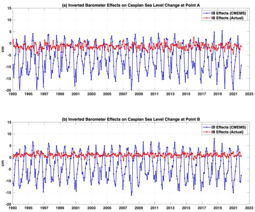
Figure 5a,b (note the different color scales used for the two maps). Annual amplitudes of the actual IB corrections over the Caspian Sea are mostly less than 1 cm, while the annual amplitudes of the CMEMS approximate IB corrections are about 7–8 cm. Some spatial variability exists in both cases, reflecting regional pressure variations over the Caspian Sea. Two grid points, A (51°E, 46°N) and B (52°E, 38°N) in the north and south Caspian Sea are selected and marked by the black “+” in
Figure 5a for IB affect time series comparisons shown in
Figure 6. The selections of the two points are arbitrary, to simply illustrate the slightly spatial variability of atmospheric surface pressure over the Caspian Sea (between the north and south in this case).
After applying the improved or actual IB corrections to the CMEMS SLA grids over the Caspian Sea, we recompute the CMEMS CSL change series and compare it with the Hydroweb CSL series in
Figure 7. The two altimeter CSL change results agree remarkably well and the discrepancies noted earlier are almost completely gone. The annual and semiannual amplitudes and phases and linear trend of the recomputed CMEMS CSL change series are estimated from unweighted least-squares fit and listed in
Table 1 (row 3) for comparisons. With the improved IB correction, the mean annual amplitude of the CMEMS CSL is increased from 8.72 ± 1.30 cm to 15.79 ± 1.30 cm, and agrees well with the Hydroweb estimates (17.03 ± 1.33 cm). The RMS of the residuals between the Hydroweb and CMEMS CSL estimates is reduced from 6.88 cm to 3.14 cm. As mentioned above, the IB correction, if implemented correctly, does not affect the CSL change estimates. To compute CMEMS CSL change, we can equivalently undo or remove the approximate IB correction applied to the CMEMS SLA grids.
At seasonal scales, the CMEMS approximate IB corrections (see the blue curves in
Figure 6a,b) are in phase with the observed CSL changes (see
Figure 2), all reaching the minimums around the start of the year. This is due to the fact the mean atmospheric pressure over the Caspian Sea is coincidentally out of phase with the observed CSL change, which also explains that the approximate or mis-modeled IB corrections only affect the amplitudes, but not the phase of the CSL change.
5. Conclusions and Discussion
We analyze satellite altimeter observed CSL changes over the period of January 1993 to December 2021 using the specially calibrated lake level data from the Hydroweb project and the global SLA grids provided by CMEMS. The two CSL series agree very well at interannual and longer time scales, but show significantly large discrepancies at seasonal and shorter time scales. The discrepancies are found to be introduced by the approximate IB corrections applied to the CMEMS SLA grids over the Caspian Sea. After applying the correct IB corrections using the ECMWF ERA5 sea surface pressure fields, the two altimeter-based CSL series agree remarkably well.
Over the 30-year period, satellite altimeter observed CSL series show a significant decreasing trend on top of strong seasonal variations. Decadal variations are also evident in CSL change. The estimated linear trends are −5.37 ± 0.11 and −5.40 ± 0.11 cm/yr for the Hydroweb and CMEMS CSL series, respectively. The annual amplitudes and phases of the two estimates are 17.03 ± 1.33 cm/266 ± 4 degrees vs. 15.79 ± 1.30 cm/267 ± 5 degrees. The CSL series show notable acceleration in the decreasing trend. For the period since 2005, the trends have increased to −8.86 ± 0.10 and −8.81 ± 0.10 cm/yr, respectively for the two altimeter CSL series.
The Caspian Sea is an enclosed water body separated from the ocean. The IB correction over the Caspian Sea or any enclosed lakes needs to be treated separately from the ocean by using the correct reference mean pressure. The actual IB effects over the Caspian Sea are significantly smaller than the approximate estimate in the CMEMS SLA grid data product. The IB effects only affect spatial variability of sea level (or lake water level), but not the average sea or water level change of the global ocean or entire water body.
Satellite altimetry has been an established space geodetic technique for measuring and monitoring the global sea level change for over three decades since the launch of T/P, the first modern satellite altimeter mission. However, accurate quantification of SLA or water level changes in lakes using a satellite altimeter is still challenging. For large lakes, such as the Caspian Sea, altimeter-derived water level changes (or anomalies) are subject to larger uncertainties due to relatively smaller spatial scales, difficulties in modeling the tides, and special implementations of atmospheric loading corrections. Climate change is taking a big toll on the Caspian Sea and the surrounding region. A long record of continuous and accurate measurements of CSL change from satellite altimetry is important for people to better understand CSL change and its connections with climate change.
Author Contributions
Conceptualization, J.C. and A.C.; methodology, J.C.; software, J.C.; validation, J.C. and A.C.; formal analysis, J.C. and A.C.; investigation, J.C., A.C., S.-Y.W. and J.L.; resources, J.C.; data curation, J.C., S.-Y.W. and J.L.; writing—original draft preparation, J.C.; writing—review and editing, J.C., A.C., S.-Y.W. and J.L.; visualization, J.C.; supervision, J.C.; project administration, J.C.; funding acquisition, J.C. All authors have read and agreed to the published version of the manuscript.
Funding
This study was supported by the PolyU SHS (Project ID: P0042322), LSGI Internal Research Funds (Project ID: P0041486), the Natural Science Foundation of China (Grant Agreement Nos. 12003057 and 11873075), and the Natural Science Foundation of Shanghai under Grant Agreement No. 20ZR1467400. This study was also partly supported by the Opening Project of the Shanghai Key Laboratory of Space Navigation and Positioning Techniques, and made use of the High-Performance Computing Resource in the Core Facility for Advanced Research Computing at Shanghai Astronomical Observatory, Chinese Academy of Sciences.
Data Availability Statement
Acknowledgments
The authors are grateful to the three anonymous reviewers for their comprehensive and insightful comments, which have led to improved presentation of the results. This work made use of the High-Performance Computing Resource in the Core Facility for Advanced Research Computing at Shanghai Astronomical Observatory, Chinese Academy of Sciences.
Conflicts of Interest
The authors declare no conflict of interest.
References
- Cazenave, A.; Bonnefond, P.; Dominh, K.; Schaeffer, P. Caspian Sea Level from Topex-Poseidon Altimetry: Level Now Falling. Geophys. Res. Lett. 1997, 24, 881–884. [Google Scholar] [CrossRef]
- Panin, G.N.; Solomonova, I.V.; Vyruchalkina, T.Y. Regime of Water Balance Components of the Caspian Sea. Water Resour. 2014, 41, 505–511. [Google Scholar] [CrossRef]
- Chen, J.; Pekker, T.; Wilson, C.R.; Tapley, B.D.; Kostianoy, A.G.; Cretaux, J.F.; Safarov, E.S. Long-Term Caspian Sea Level Change. Geophys. Res. Lett. 2017, 44, 6993–7001. [Google Scholar] [CrossRef]
- Roshan, G.; Moghbel, M.; Grab, S. Modeling Caspian Sea Water Level Oscillations under Different Scenarios of Increasing Atmospheric Carbon Dioxide Concentrations. J. Environ. Health Sci. Eng. 2012, 9, 24. [Google Scholar] [CrossRef] [PubMed] [Green Version]
- Prange, M.; Wilke, T.; Wesselingh, F.P. The Other Side of Sea Level Change. Commun. Earth Environ. 2020, 1, 69. [Google Scholar] [CrossRef]
- Nandini-Weiss, S.D.; Prange, M.; Arpe, K.; Merkel, U.; Schulz, M. Past and Future Impact of the Winter North Atlantic Oscillation in the Caspian Sea Catchment Area. Int. J. Clim. 2020, 40, 2717–2731. [Google Scholar] [CrossRef] [Green Version]
- Jackson, C.R.; Apel, J.R. Synthetic Aperture Radar Marine User’s Manual; National Oceanic and Atmospheric Administration: Washington, DC, USA, 2004.
- Intergovernmental Oceanographic Commission. Guide to Satellite Remote Sensing of the Marine Environment; UNESCO: Paris, France, 1992; p. 178. [Google Scholar] [CrossRef]
- Rani, M.; Masroor, M.d.; Kumar, P. Remote Sensing of Ocean and Coastal Environment—Overview. In Remote Sensing of Ocean and Coastal Environments; Elsevier: Amsterdam, The Netherlands, 2021; pp. 1–15. ISBN 978-0-12-819604-5. [Google Scholar]
- Hamlington, B.D.; Gardner, A.S.; Ivins, E.; Lenaerts, J.T.M.; Reager, J.T.; Trossman, D.S.; Zaron, E.D.; Adhikari, S.; Arendt, A.; Aschwanden, A.; et al. Understanding of Contemporary Regional Sea-Level Change and the Implications for the Future. Rev. Geophys. 2020, 58, e2019RG000672. [Google Scholar] [CrossRef] [PubMed]
- Cazenave, A.; Moreira, L. Contemporary Sea-Level Changes from Global to Local Scales: A Review. Proc. R. Soc. A. 2022, 478, 20220049. [Google Scholar] [CrossRef] [PubMed]
- Fu, L.-L.; Davidson, R.A. A Note on the Barotropic Response of Sea Level to Time-Dependent Wind Forcing. J. Geophys. Res. 1995, 100, 24955–24963. [Google Scholar] [CrossRef]
- Escudier, P.; Couhert, A.; Mercier, F.; Mallet, A.; Thibaut, P.; Tran, N.; Amarouche, L.; Picard, B.; Carrere, L.; Dibarboure, G.; et al. Satellite Radar Altimetry. In Satellite Altimetry over Oceans and Land Surfaces; Stammer, D., Cazenave, A., Eds.; CRC Press: Boca Raton, FL, USA; Taylor & Francis: Abingdon, UK, 2017; pp. 1–70. ISBN 978-1-315-15177-9. [Google Scholar]
- Cretaux, J.F.; Abarca Del Rio, R.; Bergé-Nguyen, M.; Arsen, A.; Drolon, V.; Clos, G.; Maisongrande, P. Lake Volume Monitoring from Space. Surv. Geophys. 2016, 37, 269–305. [Google Scholar] [CrossRef] [Green Version]
- Cretaux, J.F.; Jelinski, W.; Calmant, S.; Kouraev, A.; Vuglinski, V.; Bergé-Nguyen, M.; Gennero, M.C.; Nino, F.; Rio, R.A.R.; Cazenave, A.; et al. SOLS: A Lake Database to Monitor in the Near Real Time Water Level and Storage Variations from Remote Sensing Data. Adv. Space Res. 2011, 47, 1497–1507. [Google Scholar] [CrossRef]
- Gill, A.E. Atmosphere—Ocean Dynamics; International Geophysics Series; Academic Press: New York, NY, USA, 1982; ISBN 978-0-12-283522-3. [Google Scholar]
- Chen, J.L.; Wilson, C.R.; Tapley, B.D.; Famiglietti, J.S.; Rodell, M. Seasonal Global Mean Sea Level Change from Satellite Altimeter, GRACE, and Geophysical Models. J. Geod. 2005, 79, 532–539. [Google Scholar] [CrossRef]
- Hersbach, H.; Bell, B.; Berrisford, P.; Hirahara, S.; Horányi, A.; Muñoz-Sabater, J.; Nicolas, J.; Peubey, C.; Radu, R.; Schepers, D.; et al. The ERA5 Global Reanalysis. Q. J. R. Meteorol. Soc. 2020, 146, 1999–2049. [Google Scholar] [CrossRef]
- Copernicus Climate Change Service (C3S). ERA5: Fifth Generation of ECMWF Atmospheric Reanalyses of the Global Climate. Copernicus Climate Change Service Climate Data Store (CDS). 2017. Available online: https://cds.climate.copernicus.eu/cdsapp#!/home (accessed on 24 November 2022).
| Disclaimer/Publisher’s Note: The statements, opinions and data contained in all publications are solely those of the individual author(s) and contributor(s) and not of MDPI and/or the editor(s). MDPI and/or the editor(s) disclaim responsibility for any injury to people or property resulting from any ideas, methods, instructions or products referred to in the content. |
© 2023 by the authors. Licensee MDPI, Basel, Switzerland. This article is an open access article distributed under the terms and conditions of the Creative Commons Attribution (CC BY) license (https://creativecommons.org/licenses/by/4.0/).


