Article

Deep Clouds on Jupiter

by
Michael H. Wong
1,2,*,
Gordon L. Bjoraker
3,
Charles Goullaud
1,
Andrew W. Stephens
4,
Statia H. Luszcz-Cook
5,6,
Sushil K. Atreya
7,
Imke de Pater
1 and
Shannon T. Brown
8
1
Center for Integrative Planetary Science, University of California, Berkeley, CA 94720, USA
2
Carl Sagan Center for Research, SETI Institute, Mountain View, CA 94043, USA
3
NASA Goddard Space Flight Center, Code 693, Greenbelt, MD 20771, USA
4
Gemini Observatory, NSF’s NOIRLab, Hilo, HI 96720, USA
5
Columbia Astrophysics Laboratory, Columbia University, New York, NY 10027, USA
6
American Museum of Natural History, New York, NY 10024, USA
7
Climate and Space Sciences and Engineering, University of Michigan, Ann Arbor, MI 48109, USA
8
Jet Propulsion Laboratory, California Institute of Technology, Pasadena, CA 91109, USA
*
Author to whom correspondence should be addressed.
Remote Sens. 2023, 15(3), 702; https://doi.org/10.3390/rs15030702
Submission received: 22 November 2022 / Revised: 23 December 2022 / Accepted: 11 January 2023 / Published: 25 January 2023
(This article belongs to the Special Issue Remote Sensing Observations of the Giant Planets)

Abstract

:
Jupiter’s atmospheric water abundance is a highly important cosmochemical parameter that is linked to processes of planetary formation, weather, and circulation. Remote sensing and in situ measurement attempts still leave room for substantial improvements to our knowledge of Jupiter’s atmospheric water abundance. With the motivation to advance our understanding of water in Jupiter’s atmosphere, we investigate observations and models of deep clouds. We discuss deep clouds in isolated convective storms (including a unique storm site in the North Equatorial Belt that episodically erupted in 2021–2022), cyclonic vortices, and northern high-latitude regions, as seen in Hubble Space Telescope visible/near-infrared imaging data. We evaluate the imaging data in continuum and weak methane band (727 nm) filters by comparison with radiative transfer simulations, 5 micron imaging (Gemini), and 5 micron spectroscopy (Keck), and conclude that the weak methane band imaging approach mostly detects variation in the upper cloud and haze opacity, although sensitivity to deeper cloud layers can be exploited if upper cloud/haze opacity can be separately constrained. The cloud-base water abundance is a function of cloud-base temperature, which must be estimated by extrapolating 0.5-bar observed temperatures downward to the condensation region near 5 bar. For a given cloud base pressure, the largest source of uncertainty on the local water abundance comes from the temperature gradient used for the extrapolation. We conclude that spatially resolved spectra to determine cloud heights—collected simultaneously with spatially-resolved mid-infrared spectra to determine 500-mbar temperatures and with improved lapse rate estimates—would be needed to answer the following very challenging question: Can observations of deep water clouds on Jupiter be used to constrain the atmospheric water abundance?

Graphical Abstract

1. Introduction

Aerosol particles in the atmospheres of giant planets can be roughly divided into categories of “clouds” and “hazes,” although these terms are difficult to quantitatively define. West et al. [1] used definitions based on opacity and vertical structure, with “haze” referring to layers with low optical depth τ and possibly extended vertical structure (high particle-to-gas scale height ratio, H p / H g ). They used “cloud” to refer to regions with high τ and low H p / H g . Particle origins could also be used to distinguish clouds and hazes, with clouds formed by the condensation of volatile heavy element gas species such as water vapor, and hazes from products of chemistry driven by energy input from solar ultraviolet, auroral precipitation and heating, atmospheric electrical phenomena, cosmic rays, etc. The different origins of particles lead to an altitude-based definition, with hazes formed at pressure levels near and above the tropopause that can be reached by external energy inputs, and with clouds formed below the tropopause, where warmer air laden with volatiles mixes upward to the condensation levels of various species.
The distinction between hazes as higher-altitude phenomena and clouds as lower-altitude phenomena becomes blurred in the ice giants. Several analyses have suggested that extended hazes (in the opacity/vertical structure sense) were found in Neptune’s troposphere [2,3], supported by analysis of more recent infrared spectroscopic data [4]. Irwin et al. [5] found that hazes (in the origin sense) mix into the tropospheres of Uranus and Neptune and interact with clouds, serving as condensation nuclei and modifying the single-scattering albedo of cloud particles. This ice giant finding is relevant to the case of the gas giants Jupiter and Saturn, where haze and cloud interaction have been discussed as mechanisms to suppress the infrared spectral signatures of ammonia ice [6] or to drive color changes in anticyclonic vortices such as Oval BA [7,8]. In Neptune’s atmosphere, compact bright clouds (in the origin sense) are composed of CH 4 ice condensed at high altitudes, extending into the lower stratosphere (making them hazes in the altitude sense [9,10]). Methane comprises the highest-altitude condensation clouds on Uranus and Neptune, but in the warmer atmospheres of Jupiter and Saturn, remote sensing in the visible/near-infrared wavelength regime can detect sunlight scattered back from cloud decks of ammonia, ammonium hydrosulfide, and water (in order of increasing pressure level). Distinguishing the depths of these cloud layers, especially when multiple layers are present, is a challenging feat.
In the discussion of deep clouds inferred from imaging data in this paper, as well as deep clouds identified spectroscopically in the companion paper Bjoraker et al. [11] in this Special Issue, we conceive of deep clouds as anything within the NH 4 SH and H 2 O condensation region. We also refer to an upper cloud/haze layer, which we conceive as a combination of aerosols from NH 3 condensation, plus upper tropospheric hazes of possible photochemical origin. This categorization allows us to focus on water clouds, which are the deepest clouds potentially detectable in Jupiter’s atmosphere in reflected sunlight. The next deepest layers of thermodynamically expected condensation (KCl, ZnS) are not found until several hundred bar [12]. Rayleigh scattering and gas opacity limit sunlight penetration depths to about 20–50 bar even in the absence of other aerosols [13,14].
Identifying deep water clouds is valuable for two reasons: they are intimately connected to atmospheric circulation and heat transport via moist convection, and their depth provides a lower limit on the abundance of water in the atmosphere. Deep clouds have been identified in rare cases using imaging data (particularly using 727-nm imaging filters, as discussed in Section 2), although most of the planet’s aerosol opacity is dominated by cloud and haze particles at p < 1 bar. Remote sensing in the 5-µm infrared window has also been exploited to resolve spectral lines of well-mixed gases such as CH 3 D, which can sense deep cloud levels. Bjoraker et al. [11] used this approach to identify cloud opacity in the 4–7 bar range. The deep cloud levels can be used to constrain the water abundance at the location of the observed cloud, because saturation is implied at or below the level where cloud opacity is located. Any local water abundance must still be regarded as a lower limit to the bulk atmospheric abundance, given numerous observational and theoretical findings that volatile species in giant planet atmospheres are depleted (with respect to bulk atmospheric abundances) to vertical levels significantly deeper than their cloud bases, e.g., [4,15,16,17,18].
Water abundance is commonlyreferenced to the protosolar O/H ratio of 5.4 × 10 4 from Asplund et al. [19], corresponding to an atmospheric H 2 O/H 2 volume mixing ratio of 1.1 × 10 3 , or an atmospheric concentration (or mole fraction) of 9.3 × 10 4 in Jupiter’s atmosphere depending on the assumptions of other gas mixing ratios. Both Asplund et al. [19] and Asplund et al. [20] give the same photospheric ratios of O/H, N/H, and S/H (for elements that form clouds in Jupiter’s troposphere), but the two papers differ in the corrections for solar evolution that convert from photospheric to protosolar abundances. In this work, we use a protosolar correction of +0.04 dex [19,21], although Asplund et al. [20] reviews more recent work with corrections falling between +0.064 dex for the solar model of Vinyoles et al. [22] to as low as +0.03 dex.
The cloud-height approach is one of several approaches that have been followed in the quest to measure Jupiter’s water abundance. The sole in situ measurement is from the Galileo Probe mass spectrometer [16,23], giving a low result of 0.46× protosolar O/H, but influenced by compositional perturbations from the 5-µm hot spot at the probe entry site [24,25]. The Microwave Radiometer (MWR [26]) on the Juno orbiter [27] constrains the water abundance to 1–5× protosolar in the equatorial region [18], with further analysis and laboratory data expected to extend this determination to other latitudes in the near future [28,29]. The depth of lightning flashes was used as a constraint on O/H (using similar reasoning to the cloud-height approach, [30,31]), but the possibility of flashes extending below the water condensation level [32] means that flash depth does not directly relate to water abundance at the lightning site. Even the suggestion that 1 × protosolar water is needed so that mixed-phase cloud particles can achieve sufficient charge separation [33] is called into question by very shallow lightning detected in Juno night-side imaging, which has been explained by hypothetical mushballs composed of mixed-phased condensates with high ammonia concentration [32,34,35]. Direct spectroscopic measurements of water vapor concentration find very low mole fractions [11,36], but this could result from the same dynamical effects [37,38,39] governing the trend in ammonia from microwave remote sensing of Jupiter, which finds depletion of ammonia at depths greatly exceeding the ammonia condensation level [15,17,18,40]. Measurements of CO in the troposphere have also been used as a constraint on the O/H ratio at the deep quench level for thermochemical conversion between H 2 O and CO [41,42,43,44], but in addition to measurement uncertainties on CO, this method is sensitive to differences in the treatment of mixing and the choice of chemical network reactions and reaction rates [45,46,47,48,49]. Although our study was originally conceived as a way to narrow the uncertainty on Jupiter’s atmospheric O/H ratio, we ultimately find that the problem remains challenging, such that a range of simultaneous observations from the visible to the mid-infrared would be needed to truly derive tight constraints on O/H using the cloud-height approach. Even then, only lower limits on O/H can be established using measurements of cloud tops rather than cloud bases, unless the vertical thickness of the cloud layer can be separately determined.
We present new results on the multi-level distribution of Jupiter’s clouds, on how uncertainties in Jupiter’s temperature structure propagate to uncertainties in the O/H ratio at the cloud base, and how future spectro-imaging observations at high spatial resolution might make progress on our understanding of deep clouds. In Section 2, we use Hubble Space Telescope (HST) and Gemini North ground-based imaging data to identify deep clouds on Jupiter. This includes radiative transfer calculations characterizing the degeneracy between upper cloud opacity and the pressure level of deep clouds observed using the HST weak methane band filter (Section 2.3) and a description of specific features such as non-convecting deep clouds, a “stealth superstorm” driving intermittent convective eruptions throughout 2021–2022, deep clouds in cyclonic vortices, and a broad region north of 45°N that has a shift in the depth of cloud opacity. In Section 3, we calculate cloud base pressure levels for a suite of temperature conditions that span the full range of published data. In Section 4 and Section 5, we apply the results of the radiative transfer and cloud condensation models to specific areas of interest, discuss how the results to date constrain the atmospheric water abundance (particularly as applied to the cloud-top pressures derived in Bjoraker et al. [11]), and recommend directions for future studies to advance our knowledge of Jupiter’s deep cloud structure.

2. Imaging Deep Jovian Clouds with HST

Imaging observations of Jupiter, particularly those at high spatial resolution, provide useful constraints on the distribution of deep clouds on Jupiter. This section covers the data and the diagnostics used to constrain deep clouds in HST data, which follows approaches previously used for Galileo and Cassini imaging observations. Section 2.2 focuses on examples of deep clouds in three specific areas of interest: convective storms, non-convective deep clouds, and deep clouds at high latitudes. In Section 2.3, we quantitatively interpret Jupiter imaging data using a radiative-transfer modeling study.

2.1. Imaging Data

Visible/UV/near-IR observations were performed with the UVIS channel of the WFC3 instrument [50] on the Hubble Space Telescope. The FQ727N filter on WFC3, which samples the reflectivity in the 727-nm weak methane absorption band, is key to identifying and mapping deep clouds on Jupiter. Methane-band (and continuum) quad filters were included in the design for WFC3 with the primary intention of supporting studies of giant planet atmospheres [51].
Thermal infrared imaging was performed with the NIRI instrument [52] at the Gemini North telescope. We used the M’-band filter with a central wavelength of 4.7 µm, although we also generically refer to images at this wavelength as 5-µm images because the M’ filter is situated within the broad 5-µm window where thermal radiation from the 2–11 bar region of Jupiter’s troposphere can escape to space [11,53,54].
Figure 1 presents an overview of imaging data acquired 21–23 May, 2022 in various filters, along with composites and filter ratios. Channels have been scaled to maximize contrast (see color bars). Data were taken close in time to the Juno perijove 42 pass (diffraction-limited resolution was 300 km for HST at 727 nm and 575 km for Gemini at 4.7 µm). Data in panels B, D, E, and F are corrected for limb darkening (Minnaert k = 0.98 for 727 nm, 0.999 for other HST filters). Panel A is shown with natural limb darkening, and panel C is stretched by the 0.4 power to emphasize faint detail. Ratios in panel G are based on data without limb-darkening correction. Frames taken at different times were remapped to a common time point to reconstruct the full-disk image in each composite. See Supplemental Figures S1–S12 in SM1 for enlargements.

2.1.1. HST Imaging Programs

HST data used in this study are listed in Table 1. Although the majority of HST data are from WFC3, one figure shows an RGB composite map taken with the WFPC2 instrument in 2007. Figure 1 presents data taken near the time of Juno PJ 42. PJ stands for perijove, the Jupiter periapsis portion of the Juno orbit when atmospheric science observations are conducted. Continuum and 727-nm filter data were used to compare with radiative-transfer forward models discussed in Section 2.3. HST and Gemini data taken near Juno’s PJ 19 [55,56,57] are used in Section 4.1 to validate the interpretation of the radiative transfer modeling. HST/WFC3 data from some other epochs are also discussed, but many more epochs are not shown and merit additional detailed investigation in future work.

2.1.2. HST Data Processing

Jupiter maps result from images that have gone through several stages of processing, as described in detail in [55]. These stages involve cleaning of cosmic ray artifacts, correction of geometric distortion, photometric calibration to I / F (reflectivity) units [4], and navigation to transform the data to latitude/longitude coordinates on Jupiter. (Planetographic latitudes are used in this paper unless otherwise noted.) Corrections for fringing (etaloning) artifacts in the narrow-band filters at λ > 700 nm were performed [58]. The WFC3 pipeline now includes time-dependent photometric calibration [59].
Processing of the WFPC2 data was discussed in Asay-Davis et al. [60].

2.1.3. Gemini Imaging Data and Data Processing

Figure 1C presents M-band (4.7 µm) imaging data taken with the NIRI camera at Gemini Observatory. The data were taken near Juno PJ 42 on 23 May 2022 between 14:39 and 14:50, using a four-position mosaic. To approach the diffraction limit of the telescope, individual 0.3-sec exposures were coadded in a lucky-imaging approach described in Wong et al. [55]. To assist in comparison with HST imaging in Figure 1 taken almost four Jupiter rotations earlier, refer to individual features marked on the images at the two time-points in the Supplementary Material. Gemini data presented in later figures were taken near Juno PJs 19 and 29.

2.1.4. Cloud Depths from Imaging

A wide range of filters across the visible spectrum have been used to constrain cloud vertical structure. Because structure varies significantly on short length scales, the high resolution provided by spacecraft (and HST) imaging data is required, particularly within discrete features. For constraining the deepest clouds, a filter pair measuring the reflectivity in the 727-nm weak methane band plus reflectivity in a nearby continuum wavelength are most effective [55,61,62]. Prior works have visually represented the resulting cloud depth information in two ways, for which we adopt specific convenience labels in this work:
CH 4 composites, or CH 4 -band cloud depths maps (e.g., Figure 1B). These are a standard type of color composite image, where the red/green/blue channels of the composite are used to display, respectively, the deep-probing continuum/weak CH 4 band (727 nm) / strong CH 4 band (889 nm). Examples of CH 4 -band depth maps from Galileo Orbiter data are shown in Figure 6 of Banfield et al. [61] and Figures 1 and 2 of Gierasch et al. [63]. Examples from Cassini data are shown in Figures 2 and 3 of Porco et al. [62] for Jupiter, and Figure 4 of Sayanagi et al. [64] for Saturn.
In this paper, we use either 631-nm or 750-nm filters as “continuum” reference filters for the weak methane band at 727 nm. Neither filter provides a perfect continuum reference. The WFC3 FQ750N filter is officially the continuum filter for FQ727N [50], but its use is complicated by the presence of NH 3 gas absorption within its bandpass [14]; see Section 2.3 below. The disadvantage of the F631N filter is the greater wavelength shift compared to 727 nm (13% rather than 3% for 750 nm), which allows particle properties to influence the relative reflectances.
CM7 is an abbreviation used in this article for the ratio of the continuum to methane 727-nm reflectivity:
CM 7 = I / F cont . I / F 727
The CM7 ratio is useful for distinguishing deep clouds from upper clouds in Jupiter’s atmosphere (e.g., Figure 1G). Continuum filters reach an optical depth of 1 (for two-way scattering/absorption of sunlight back to the observer) near 6–10 bar in an aerosol-free atmosphere [65], while the weak CH 4 -band filter near 727 nm reaches two-way τ = 1 near 3 bar, and the strong CH 4 -band filter near 889 nm reaches two-way τ = 1 near 300–500 mbar [61]. When the vertically integrated aerosol opacity has a stronger contribution from deep clouds, CH 4 absorption in the in 727-nm bandpass limits the response in the weak methane-band filter, so the CM7 ratio is higher. Low values of CM7 correspond to cloud structures dominated by upper-level opacity, or structures with very high upper-level opacity such that both filters are insensitive to any deeper clouds. The CM7 ratio is sensitive to the relative weighting between upper opacity and deep opacity in the column, but the ratio is insensitive to the total amount of opacity.
The CM7 ratio was used in Figure 5.9 of West et al. [66] to identify deep clouds in a region of active moist convection. The imaging data constrained the deep clouds to lie at pressures of 3 bar or deeper, leading West et al. [66] to conclude that the clouds must be composed of water, since NH 3 and NH 4 SH cannot condense as deep in the atmosphere. The CM7 ratio safely avoids division by zero because even in locations with no condensation clouds, Jupiter’s reflectivity is nonzero due to Rayleigh scattering and scattering by low-opacity hazes at high altitudes. The continuum wavelength used in the ratio varies, depending on the filters available at a given observation time.
Quantitative interpretation of cloud depth using narrow-band imaging data requires radiative transfer analysis, as described in Section 2.3. However, qualitative information can be derived from simple visual comparison, as a demonstration of the cloud depth information content in the data.

2.2. Settings of Deep Clouds

Deep clouds on Jupiter—whether identified using the red appearance in CH 4 -band composites, high CM7 ratios, or CH 3 D line widths in high-resolution 5-µm spectroscopy [11]—are often located in three distinct settings: isolated moist convective storms, cyclonic vortices, and a large region north of 45°N with distinct cloud structure. In this section, we discuss specific observations of deep clouds in each of these three settings.

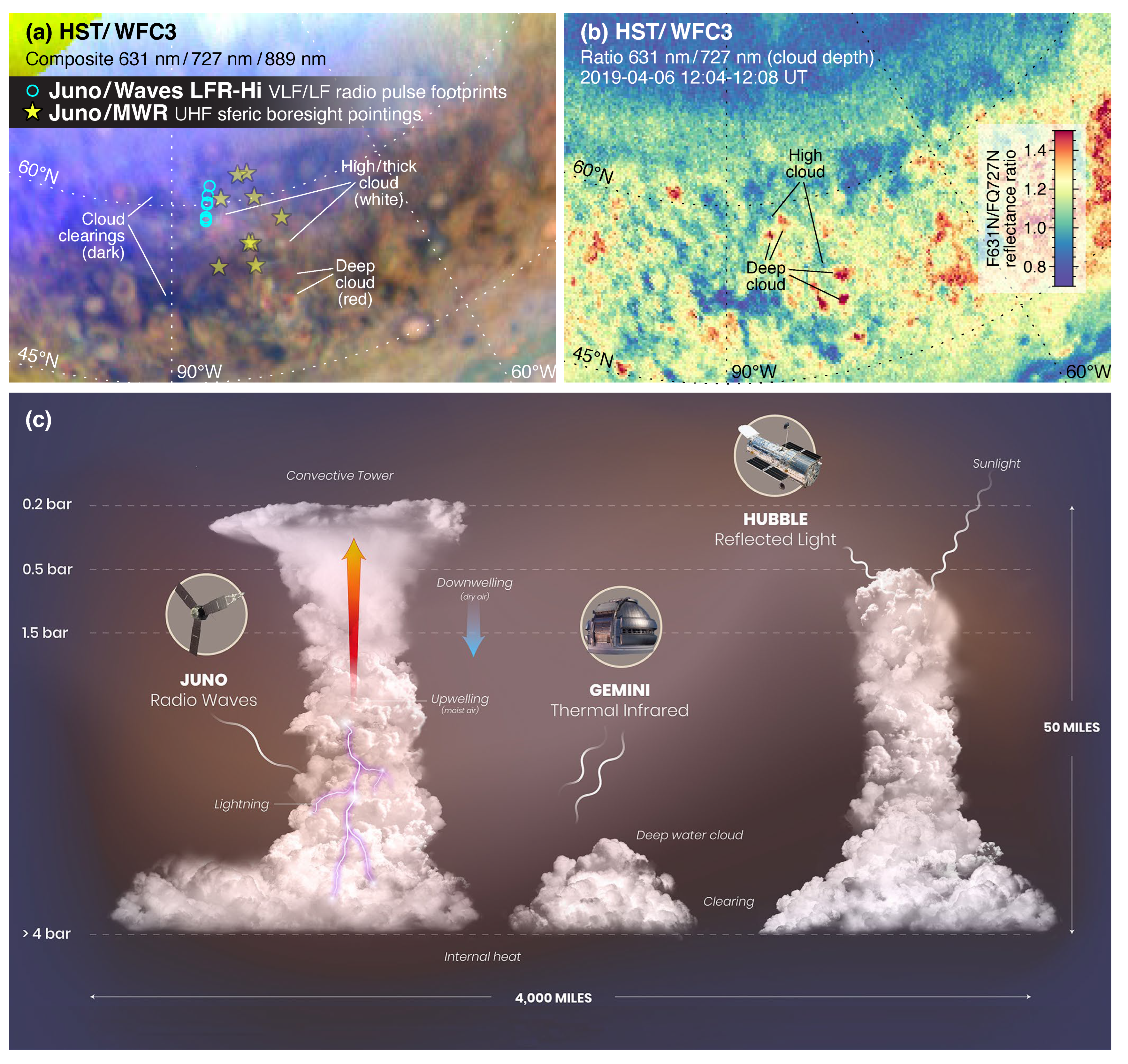
2.2.1. Deep Cloud Setting 1: Moist Convective Storms

The cloud structure in moist convective systems has been investigated on Jupiter for decades. Gierasch et al. [63] used Galileo imaging data to identify a two-component cloud structure in a region of active moist convection: (1) deep water clouds juxtaposed with (2) thick convective towers reaching high altitudes. Night-side imaging detected lightning within the cloud complex, confirming its moist-convective nature. The cloud structure was derived from CH 4 -composite maps.
Imai et al. [56] identified a third component of the cloud structure in active moist convective regions: cloud clearings (Figure 2). As with Gierasch et al. [63], Imai et al. [56] combined lightning detections with CH 4 -band cloud depth maps, but in this case, the lightning came from localized signals detected by Juno in the microwave/radio wavelength regime, and the cloud depth maps came from HST imaging data.
Galileo night-side imaging found lightning flashes in the North Equatorial Belt (NEB) among other locations (e.g., Storm 15 in Figures 3 and 4 of Little et al. [67]). Around the time of Juno’s perijove 28 in July 2020, HST imaging revealed a series of deep clouds in the NEB, but Juno did not detect lightning near the deep clouds. HST images three days prior (Figure 3, left) showed deep clouds juxtaposed with tall/thick convective towers and cloud clearings (the three-component cloud structure characteristic of active moist convection). However, by the time Juno scanned the same deep clouds, the tall/thick cloud towers had disappeared, suggesting that moist convective activity had ended. Three days is long enough to observe significant evolution in a moist convective storm, although denser temporal sampling would be needed to fully characterize timescales of storm evolution. The 10-hour cadence of the Cassini Jupiter-approach time series (see Figure 3 of Porco et al. [62]) confirms three days to be the approximate timescale for the decay of a convective storm eruption in the region to the northwest of the Great Red Spot (GRS). As with Figure 3, compact deep clouds remained after the decay of tall convective towers. Isolated compact deep clouds may commonly persist for a longer time than active convective outbreaks.
In 2021 and early 2022, typical isolated convective storms in the NEB such as those in Figure 3 died out, except at a single active latitude that drifted around the planet at a constant speed [69,70]. Figure 4 shows the cloud structure around the active longitude in May 2022, near Juno perijove 42 (PJ 42). Juno MWR measurements of lightning activity near the same active longitude several months prior (near perijove 38) suggest that storms near the active longitude are moist-convective in nature, yet the cloud structure in Figure 4 is not fully consistent with the three-component moist convective cloud structure. Specifically, deep clouds (red in a CH 4 composite) are largely absent near the active longitude, whereas typical moist-convective storms feature deep clouds and tall, thick clouds with roughly equal feature sizes and areal coverage. Reflectivity in the strong methane band (889 nm) is also not particularly strong relative to nearby cloud features, suggesting weak convection that does not extend to high tropospheric levels. There is no clear explanation why convection in the NEB in 2021–2022 exhibits the long-term behavior typical of a large superstorm while the cloud structure is barely consistent with moist convection and the cloud tops do not reach the same heights typical of other moist-convective regions.

2.2.2. Deep Cloud Setting 2: Cyclonic Vortices

Deep clouds detected within some cyclonic vortices may be examples of clouds formed without strong moist convective activity. Cyclonic vortices are known to transform between different morphologies: a “barge” morphology characterized by a distinct, smooth elliptical outline (e.g., Figure 5) and turbulent morphology with a less distinct peripheral boundary and a more chaotic and filamentary appearance [55,72,73,74]. Cyclone morphology transformations have been studied from the Voyager era to the Juno era [75,76,77]. The visual appearance of cyclones suggests that the folded filamentary morphology coincides with active moist convection, while the smooth-edged “barge” morphology indicates an absence of active moist convection. Figure 5 supports this interpretation because the large barge-type cyclone at the center of the map lacks key elements of convective cloud structure (tall/thick cloud towers and deep clearings), while folded filamentary cyclones have all three components of convective cloud structure [55]. Additionally, Wong et al. [55] linked clusters of lightning sferics detected by Juno MWR to folded filamentary regions (FFRs), while the barge in Figure 5A is not accompanied by a cluster of lightning signals. Some lightning directly to the north is found much closer to regions exhibiting the three-component cloud structure signature of moist convection. Bolton et al. [57] analyzed MWR scans of this particular barge, finding a density inversion layer somewhere in the 3–6 bar range. The observation of a deep central cloud suggests that convection in the water cloud layer is taking place, but perhaps the density inversion layer represents strong convective inhibition (CIN [78]), preventing the moist convective process from rising up to the upper troposphere, as seen in FFRs.
A barge in the South Equatorial Belt was imaged by HST/WFPC2 in 2007 (Figure 5B), revealing a compact central red cloud in RGB composite (pseudo true color) images [79]. Deep clouds can appear red in RGB composites because Rayleigh scattering limits the penetration depth of sunlight at short wavelengths. The barge with the central red cloud erupted into a convective outbreak several days after the WFPC2 observations, leading to global-scale changes in cloud color at that latitude.
The creation of deep isolated clouds, particularly within non-convective cyclonic vortices, may indicate the development of conditions favoring moist convective initiation (e.g., a buildup of convective available potential energy, or CAPE [80]). Thus, deep clouds may precede moist convective outbreaks in cyclones, as well as persisting after them (as in the isolated convective storms shown in Figure 3).
Figure 6 presents an enlargement of a southern hemisphere region from Figure 1. Two cyclones are seen in different states: C45 has a smooth cigar-shaped outline with homogeneous internal cloud coverage (a “cloudy oval” state), and C34 has a folded filamentary cloud structure typical of active moist convection. The cloud structure state of C45 differs from barges because it has significant cloud opacity throughout its interior, but it shares the smooth outline of barges, unbroken by active moist convective filaments, towers, and clearings. The cloudy oval state of C45 resembles that of a named cyclone at 24°S, the South Temperate Belt Ghost, which was observed transitioning through a convective outbreak into an FFR state [76]. Hueso et al. [77] reported on two cyclones near 31°S, DS6 and DS7. DS7 (also known as Clyde’s Spot [81]) transitioned between a barge-like state and an FFR state, while DS6 transitioned between a barge-like state and a smooth-outlined but cloudy state, like the cyclone C45 in Figure 6. Although it is clear that the difference between the FFR state and both of the smooth-outline cyclone states (barge and cloudy oval states) is active moist convection, it is not clear whether the cyclone’s internal structure or its interactions with surrounding cloud layers explains the differences between barge states (Figure 5) and cloudy oval states (Figure 6). Deep clouds have been seen within cyclones in FFR and barge states, but the high opacity of upper-level clouds in the cloudy oval cyclone state prevents detection of any deeper clouds that may lie beneath the upper aerosol layer.

2.2.3. Deep Cloud Setting 3: The Northern High Latitudes

Past studies of Jupiter’s cloud structure have naturally concentrated on low latitudes, where the view from Earth is least distorted. However, recent attention has been drawn to the high latitudes, particularly in the northern hemisphere, due to the data coming from Juno on its polar orbit (Figure 7).
Figure 8 shows a systematic difference in cloud properties above and below 45°N in observations taken in 2020. Specifically, the CM7 ratio is higher north of 45°N, which could be interpreted as deeper clouds. The presence of moist convection and thus water clouds is confirmed by numerous detections of lightning sferics from Juno/MWR data [82] north of 45°N. The dramatic drop in sferic detection rate south of 45°N requires further analysis, because spatial coverage is not uniform over the map area shown in Figure 8. The cloud structure boundary near 45°N persisted into 2022, as shown by the data in Figure 1.
Interpreting the observations requires careful attention to two questions: Could the 45°N boundary be explained by differences in viewing geometry (i.e., a higher slant angle approaching the pole)? Is there an opacity change in the upper tropospheric layer, the deep cloud layer, or both?
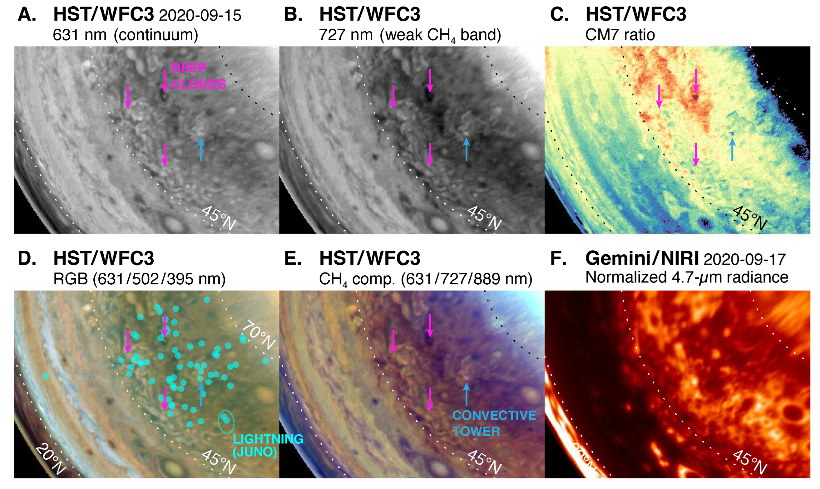
  • Viewing geometry: The boundary near 45°N cannot be solely an effect of viewing geometry, based on the data in Figure 1. The CM7 ratio (Figure 1G) increases at high emission/incidence angles, raising the possibility that the 45°N boundary may be a viewing effect. However, at any fixed latitude, the CM7 ratio only increases noticeably at emission angles greater than 65 °, whereas the distinct high-latitude region begins at a much lower emission angle (roughly equivalent to the planetographic latitude). Secondly, the enhanced contribution from hazes at high viewing angles, combined with increased haze densities approaching the auroral region, should increase the 727 nm reflectivity more than the continuum, so we would expect the CM7 ratio to actually decrease towards the poles as a geometric effect. Therefore, there is strong evidence that the observed CM7 enhancement north of 45°N represents a physical change to the aerosol structure. This is further supported by evidence for a brightness enhancement of the region in at 4.7 µm in Figure 1, Figure 7, Figure 8, as well as Figure 20 in Section 4.1.
  • Separating upper/deep cloud opacity contributions. Although high CM7 values may suggest deeper clouds north of 45°N, radiative transfer modeling is needed to confirm whether upper and lower cloud opacity effects can be separated (next section). The role of upper cloud/haze opacity can be seen immediately in the 727-nm frame itself, which is darker north of 45°N, even after Minnaert correction (Figure 1E, Figure 8B). The drop in continuum reflectivity is less pronounced. The 5-µm images show enhanced thermal emission, but this wavelength is sensitive to integrated cloud opacity in both deep and shallow layers. Overall, qualitative analysis suggests a significant depletion of upper cloud/haze opacity, coupled with moderate deep cloud opacity (because even 5-µm bright regions in the high northern latitudes are not as bright as in low-latitude locations such as hot spots in the NEB).

2.3. Radiative Transfer Modeling

Remote sensing imaging data can cover a global-scale area, at spatial resolutions as fine as 230 km on Jupiter (near solar opposition), which the previous section showed is important for the study of deep clouds. Mapping the CM7 ratio (Equation (1)) in imaging data is a powerful way to identify and characterize areas and features with differences in cloud structure. Spatially resolved spectroscopy spanning the 727-nm feature has more power to derive full vertical profiles of aerosol properties, e.g., [14,84,85]. However, imaging data at fine spatial resolution can be obtained rapidly on a global scale, a capability that is not yet matched by imaging spectrometers with seeing limited resolutions of >1200 km (which averages across regions with heterogeneous cloud properties). Both imaging and spectroscopic approaches are valuable, but maximizing the return of useful vertical information on aerosol structure from imaging data requires simplifying assumptions in aerosol distributions, along with honest characterization of unavoidable systematic sources of error inherent to the more limited spectral information content available from imaging.
To better understand the vertical information that can be extracted from high-resolution imaging in 727-nm and continuum filters, we performed an exploratory radiative transfer study. The main goal of the study was to understand the amount of information available on the pressure levels of deep clouds. Recognizing that a full aerosol structure retrieval on inhomogeneous regions with small deep cloud features is underconstrained by a simple pair of narrow-band filters, we chose a forward-modeling approach to study the problem. We chose an aerosol layer framework guided by prior spectroscopic studies in the visible wavelength region, informed by the classic aerosol structure of West et al. [1,66], which contains the deep condensation clouds of interest (NH 4 SH, H 2 O), along with haze distributed in multiple upper layers. Figure 9 schematically illustrates the individual aerosol layers in our model framework. Of key importance is the upper cloud/haze layer, which we conceptualize as a combination of NH 3 condensation clouds and upper tropospheric hazes, with variable opacity. Two additional haze layers as described below were kept fixed in all model cases: a thin stratospheric haze and a vertically and optically thin layer of absorbing “chromophore” particles. The results of our study will show that there is valuable—but degenerate—information about the deep cloud levels in the spectrum, because the upper cloud/haze layer dominates the information content at these wavelengths.
We use the SUNBEAR code to forward-model a range of aerosol structures as they would be observed across the Jovian disk. The SUNBEAR (Spectra from Ultraviolet to Near-infrared with the BErkeley Atmospheric Retrieval) code is described in Molter et al. [87] and has been applied previously (but without the catchy name) to the atmospheres of Titan, Uranus, and Neptune [4,40,88,89,90,91,92]. It uses the discrete ordinates method to solve the radiative transfer equation [92,93], and treats processes important at visible wavelengths such as Rayleigh scattering, Rayleigh polarization, and Raman scattering [94,95,96,97,98,99,100]. However, Fry and Sromovsky [65] argued that these effects are not significant longward of UV wavelengths, so computational efficiency was increased by disabling these options in our study of red/near-IR wavelengths. The correlated-k approach [101] is used for gas absorption, with methane coefficients from Karkoschka and Tomasko [102] and ammonia coefficients from Irwin et al. [103]. Ammonia absorption was modeled using a vertical profile roughly consistent with Li et al. [17] and de Pater et al. [15] at p 500 mbar, decreasing with altitude to a concentration of 10 12 near the tropopause (consistent with the 80-mbar value retrieved from UV spectroscopy [104]). The model extended from a lower boundary of 26 bar to an upper boundary at 0.2 mbar, with an adaptive grid of 130 layers providing balanced vertical resolution in log-pressure space.
We wish to use CM7 values across the disk of Jupiter to interpret cloud depths, but the CM7 photometric ratio is also affected by viewing geometry. Specifically, the 727-nm reflectivities come from shallower depths when there is a greater slant angle for incoming solar radiation and outgoing scattered light, and the atmospheric scale height changes with latitude due to Jupiter’s rotation and oblateness. To test the influence of geometrical effects on the observed CM7 ratio, we performed radiative transfer model calculations over the grid of values shown in Figure 10.
Reflectivities in continuum and 727-nm filters were calculated for each point in the geometric grid. A series of six aerosol structure frameworks were tested until one was found that could approximate the reflectivities, limb darkening, and CM7 values in the HST observations (Figure 1). This adopted framework (Figure 9 and Table 2) had deep clouds placed below a “crème-brûlée” upper cloud/haze layer, with parameters broadly consistent with several recent radiative transfer analyses of spectral data in the visible range [65,84,85,86]. Crème-brûlée models get their name from an upper tropospheric haze structure that has an optically thin absorbing layer overlying an optically thicker layer with conservative scattering. We performed calculations to quantify the effect of a limited number of variables: opacity in the upper cloud/haze layer, opacity in the deep cloud layer, and pressure level of the deep cloud layer.
The rationale for parameter choices (Table 2) is as follows:
  • Stratospheric haze: A vertically extended but optically thin upper layer of small non-absorbing particles is required to match center-to-limb curves at high incidence and/or emission angles. Parameters for this layer were held fixed for all calculations shown in this paper. Values were chosen to broadly match values found in several recent works that used constraints provided by spectroscopy and/or zonal-mean center-to-limb brightness variation [65,85,86]. These works found spatially variable stratospheric haze parameters, but to simplify our investigation into deep clouds using only continuum and 727-nm narrowband filters, we kept stratospheric haze parameters fixed in all model runs.
  • Chromophore haze: A thin layer of small absorbing particles in the upper troposphere; the crème-brûlée crust. Parameters for this layer were held fixed for all calculations. The layer is moderately compact in the vertical direction. The index of refraction set to 1.4 + i0.1, generally consistent with the chromophore material characterized by Carlson et al. [105], which was an irradiated product of C 2 H 2 and NH 3 successfully used to model Jupiter’s visible-wavelength spectrum in recent work [14,65,84,85,86]. Other chromophore candidates have similar absorption characteristics, and it is difficult to identify Jupiter’s chromophores based on the planet’s spectrum alone [66,106,107].
  • Upper tropospheric cloud/haze: A non-absorbing cloud/haze layer in the upper troposphere; the custard part of the crème-brûlée. We chose representative particle characteristics with some haze-like properties (moderately small radius, puffy distribution with large H p / H g across the vertical layer), but with relatively large optical depths that might be more consistent with condensation clouds. A large H p / H g within the uppermost high-opacity layer has been suggested going back to the earliest analyses of methane absorption in the visible/near-IR spectral range [108,109]. Our simple treatment of the uppermost high-opacity layer is meant to simulate more complex but degenerate mixtures haze/cloud opacity bounded between the ammonia cloud base and the tropopause. Absorption was modeled as being concentrated in the fixed chromophore layer, so the index of refraction of this upper tropospheric cloud/haze layer was fixed at 1.4 + i10 8 . The base pressure level p base of this layer was found to have minimal influence compared to the total opacity, when p base was varied over the 300–800 mbar range (keeping the fractional scale height fixed at 1 and the low-pressure cutoff fixed at 300 mbar). The variable parameter for this layer was total optical depth τ haze (tested at 1, 3, 5, 10, and 15).
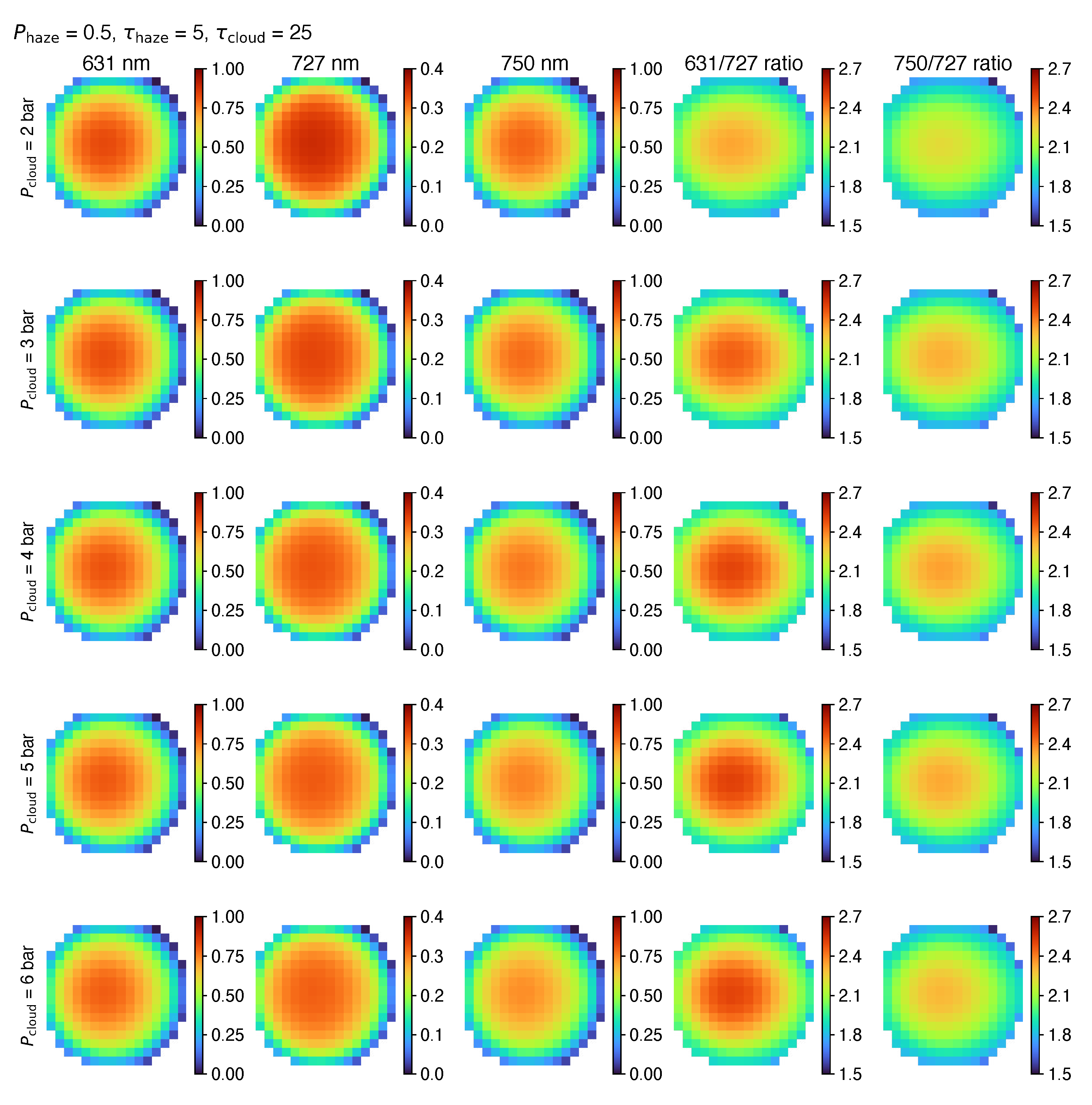
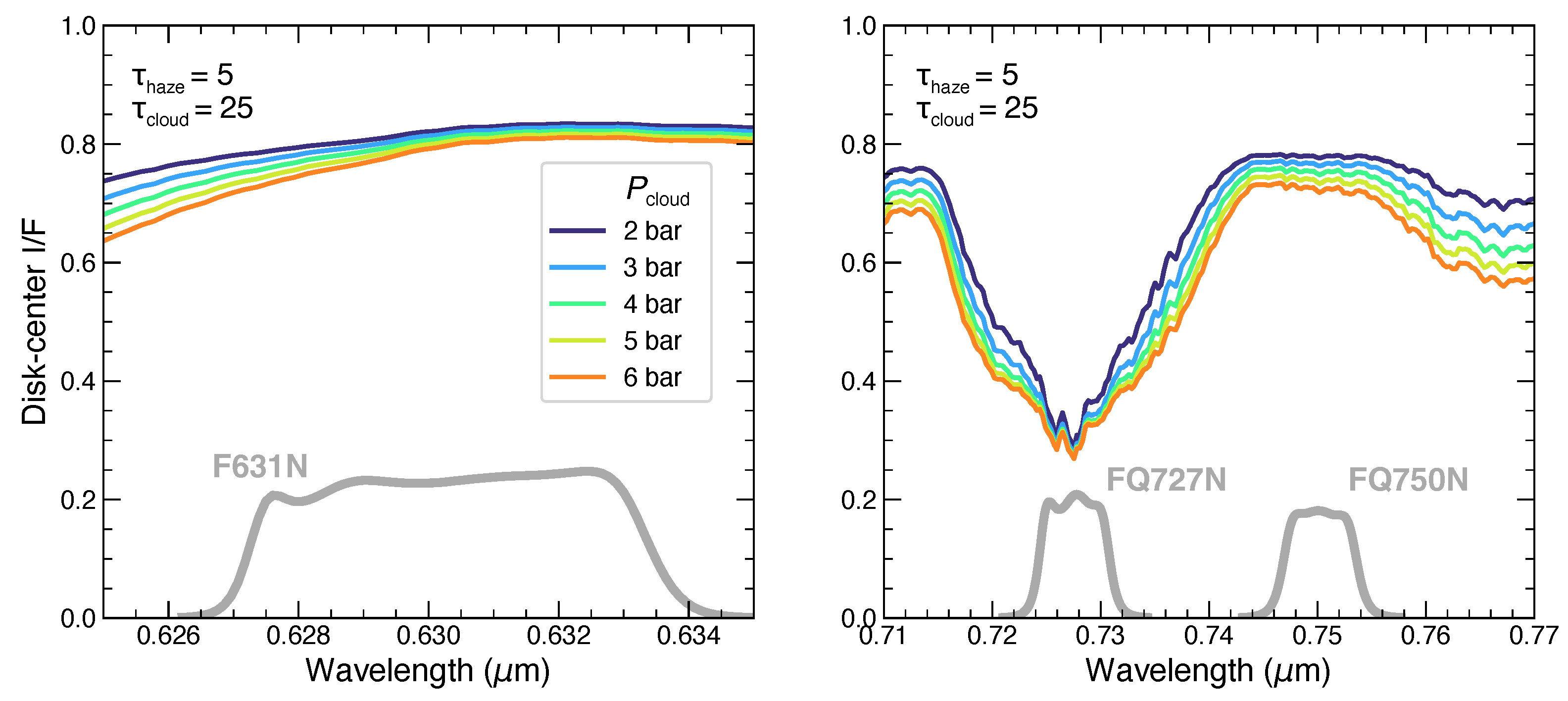
  • Deep cloud: This layer was intended to simulate NH 4 SH or H 2 O cloud opacity. To simulate a vertically-compact condensation cloud layer, we distributed the aerosol opacity above a variable cloud base with fractional scale height 0.1 and a low-pressure cutoff of p top = 0.9 × p base . Although p cloud is the model parameter, at high optical depths, it is really the cloud top that is significant, but for the vertically compact clouds assumed in the model, these agree to within 10%. The variable parameters for this layer were cloud base level p cloud (tested at 2, 3, 4, 5, and 6 bar) and total optical depth τ cloud (tested at 0, 5, 25, and 100).
The total number of model states is 5 × 5 × 3 + 5 = 80 model parameter combinations, evaluated over 224 spatial grid points (less than 16 × 16 because Jupiter is not square), or 17,920 states. Figure 11 demonstrates how model output varies over the geometrical grid and over the range of p cloud values, for cases fixed at τ haze = 5 and τ cloud = 25 . Similar plots for other τ haze and τ cloud states (not shown) can be generated using data files included in Supplemental Materials SM2.
Figure 11 shows the simulated Jupiter disk for a given cloud structure state, but this type of output is difficult to compare with observations where cloud structure is clearly variable over the disk. To better compare with the data, we sampled the Jovian disk in Figure 1 to calculate mean, maximum, and minimum values of reflectivities and CM7 ratios as a function of incidence angle cosine μ 0 . The observational data (reflectivities in 727-nm and continuum filters) are shown in black in Figure 12 (solid for the mean and dashed for the extrema at each μ 0 bin). Model output shown as colored symbols span the full geometrical grid and 15 model states, as indicated by legends in the panels. Figures S13–S17 in SM1 show all the other model states for comparison, but the states shown in Figure 12 span the full range of the observed I / F data (i.e., the colored dots span the range between the dashed black curves).
Some conclusions can be drawn already from the limb-darkening curves in Figure 12 before proceeding to discussing CM7 ratios.
The minimum reflectivities in the observations (lower dashed black lines in Figure 12 corresponding to the data in Figure 1) are best fit by the row with τ haze = 3 and τ cloud = 5 . Figures S13–S17 show that no other cloud structure provides a better fit to the minimum reflectivities: lower τ haze produces values of I / F 727 much lower than the observations, except if τ cloud at 2 bar is increased to compensate, but that then drives I / F cont . too high. Higher τ haze produces values of I / F 727 higher than the observations, even with τ cloud = 0 . One red flag is that modeled I / F 631 and I / F 750 do not both fit the lower dashed line in Figure 12 for any singular model. This could be an artifact of modeling the chromophore haze with a constant n i as a function of wavelength. The observations require a minimum optical depth of 8 (distributed among the upper cloud/haze and the lower cloud decks (at least for the assumed particle size distributions)).
The mean I / F values (solid black lines in Figure 12) are best fit by the middle row with τ haze = 5 and τ cloud = 25 . Here, the model suggests some sensitivity to the deep cloud base level p cloud (with colored points shifting from blue to orange as cloud level increases from 2 to 6 bar). For 727 and 750 nm, the mean I / F center-to-limb curve is best fit when the deep cloud opacity is located at 2 bar.
The modeled I / F at 631 nm behaves as would be expected for a continuum wavelength: it has sensitivity to the opacity of the deep cloud layer, but almost no sensitivity to the deep cloud pressure level. The sensitivity to the cloud base level in the 750-nm filter is somewhat surprising, given the official title of the FQ750N filter, “7270 continuum” [50]. Continuum filters near 750 nm were also used on Galileo and Cassini imaging systems [110,111]. Figure 5 of Sromovsky et al. [14] suggests that ammonia absorption at 750 nm may complicate the use of this filter as a continuum reference for 727 nm. In both Figure 11 and Figure 12, I / F at 750 nm decreases as p cloud increases, consistent with gas absorption in the bandpass. Figure 13 shows the model spectra across the filter bandpasses, for a single disk-center case with τ haze = 5 and τ cloud = 25 . Although the spectrum does exhibit nice continuum behavior over most of the 631-nm filter bandpass, the spectral proximity to the 619-nm methane band introduces some sensitivity to deep cloud pressure level in the blue end of the bandpass.
Finally, the bottom row of Figure 12 provides the best match to the maximum I / F center-to-limb curve for the three filters, with τ haze = 10 and τ cloud = 100 . Despite the high upper cloud/haze opacity, some sensitivity to p cloud remains due to the very high value of τ cloud = 100 required to match the maximum reflectivities. Better fits are found for p cloud = 2 bar than for deep clouds at higher pressures, so it is possible that a model with more freedom might prefer clouds within the 1–2 bar region. However, we did not test this type of cloud structure because cloud condensation efficiency is reduced at this level, according to theoretical arguments discussed in Section 3.
No attempt has been made in this work to fit differences in cloud structure within different latitude bands. In a global sense, best fit mean and minimum/maximum center-to-limb reflectivity curves are consistent with variation in the upper cloud/haze opacity from τ haze = 3 to 10, along with variation in deeper cloud opacity over a wider range of values and some sensitivity to the pressure level of the deep cloud.
For the best-fit cases (minimum, mean, and maximum I / F vs. μ 0 ) in Figure 12, we plotted the corresponding CM7 values in Figure 14.
The simulated CM7 values for moderate incidence angles ( μ 0 > 0.4) for the best-fit aerosol structures lie within the minimum/maximum observed CM7 envelope (dashed lines). In this sense, the modeled aerosol structures are Jupiter-like.
Consider first the bottom row, for the case of τ haze = 10 and τ cloud = 100 best matching the maximum I / F values in Figure 12. This case also best matches the minimum CM7 values across the disk, validating the interpretation that low CM7 corresponds to high opacity in the upper cloud/haze layer. The high upper cloud/haze opacity renders the CM7 ratio completely insensitive to p cloud . Some sensitivity to deep cloud opacity starts to appear at lower τ haze (middle row).
A degeneracy can be seen between the p cloud and τ haze parameters in Figure 14. Moving the deep cloud level upwards (decreasing p cloud , colors going from orange to blue) acts to lower the CM7 ratio. However, increasing the opacity in the upper layer also lowers CM7 (top row toward bottom row).
Taken together, the three rows show that although the CM7 ratio may be sensitive to the deep cloud level, the sensitivity to upper cloud/haze opacity dominates, and deep clouds can only be distinguished in regions where the upper cloud/haze opacity is near its minimum value. Minimum cloud/haze opacity is found where the I / F values for all filters are the lowest (Figure 12), and where CM7 is the highest. So the best place to distinguish deep clouds on Jupiter would be a location that is dark overall, with small regions where CM7 increases in discrete features located within a broad area with low τ haze . In Figure 1, Figure 3 and Figure 8, these conditions are seen to apply very well at high northern latitudes and in the NEB. Figure 15 shows simulated I / F and CM7 for a case that is still marginally consistent with the observations and that provides maximum sensitivity to cloud depth: the τ haze = 3 and τ cloud = 100 case.
The τ haze = 3 and τ cloud = 100 case is Jupiter-like because it still fits within the I / F minimum/maximum envelope for the data in Figure 1. This case provides maximum sensitivity to p cloud at disk center: when the cloud base goes from 2 to 6 bar, Δ CM 7 > 0.6 for the 631/727 ratio, and Δ CM 7 > 0.4 for the 750/727 ratio. This sensitivity to p cloud is similar to the sensitivity to τ haze in a different case ( τ cloud = 0 ; see top rows of Figures S19 and S20), where increasing τ haze from 3 to 5 gives Δ CM 7 < 0.6 for the 631/727 ratio, and Δ CM 7 < 0.2 for the 750/727 ratio. If regions of Jupiter can be identified where the upper layer opacity is inferred to remain constant (perhaps by exploiting the correlation between CM7 ratios and 889-nm I / F in imaging data, or by resolved spectroscopic observations), then variation in CM7 can be attributed to the deep cloud layer. Comparison of Figure 14 (top row) and Figure 15 reveals a serious degeneracy even in this low τ haze case, between deep cloud opacity and deep cloud pressure level. The degeneracy is worse for the 750/727 ratio, but for the 631/727 ratio, the CM7 vs. μ 0 curves have only a weak dependence on τ cloud for p cloud = 2 bar. Imaging data seem to be minimally capable of distinguishing between 2-bar and deeper clouds (under some conditions), which would be sufficient to rule out NH 4 SH composition (but not sufficient to place meaningful limits on the O/H ratio).
Although trends in the simulated data allow valuable conclusions to be drawn, the main conclusion is that variation in upper-layer cloud/haze opacity is the dominant control, such that deep cloud properties can only be constrained if the upper-layer opacity is separately measured by additional data. Beyond the challenges presented by this degeneracy, there are deficiencies in the fidelity of our aerosol model framework. One issue is that the 631-nm reflectivity is anomalously high compared to the longer-wavelength filters, a possible effect of inaccurate assumptions for the chromophore haze layer in the model. The issues with modeled 631-nm I / F can be seen in the top row of Figure 12, where a model in our framework matching the minimum observed I / F at 631 nm produces I / F far too low at the other wavelengths. Excessive 631-nm I / F means that no CM7 values in our models actually match the lowest observed CM7 values (lower dashed curves in Figure 14) at the disk center.
The second red flag is the slope of the CM7 vs. μ 0 curve, which is positive in the model but flat or slightly decreasing in the observations. Examination of the middle column of Figure 12 suggests that the CM7 slope mismatch is due to the wrong limb darkening behavior at 727 nm in the simulations. No other models tested in this work were able to achieve better matches to both the 727-nm limb darkening and overall reflectivity.
Although improved models of deep cloud reflectivity may be attempted in the future—preferably with additional information from visible-wavelength spectroscopy—the model presented here provides a reasonably close approximation to Jupiter’s reflectivity at 727 nm and adjacent continuum wavelengths, sufficient for demonstrating the strong degeneracy between the effects of upper and lower cloud opacity on the observed results.
Table 1. HST Jupiter observations used in this study.
Start Time (UT)ProgramHST Instruments and Filters UsedFigure Numbers
2022-05-22 23:32GO-16913WFC3/UVIS: F395N, F502N, F631N, FQ727N, FQ750N, FQ889NFigure 1, Figure 4, Figure 6 and Figures S1–S12
2019-04-06 10:39GO-15665WFC3/UVIS: F631N, FQ727N, FQ889NFigure 2, Figure 5, Figures 19 and 20
2020-07-22 08:19GO-16053WFC3/UVIS: F631N, FQ727N, FQ889NFigure 3
2007-05-11 12:16GO-10782WFPC2/PC1: F410M, F502N, F673NFigure 5
2020-09-15 16:33GO-16074WFC3/UVIS: F395N, F502N, F631N, FQ727N, FQ889NFigure 8
Table 2. Aerosol model framework and key parameters. Opacity in each layer is bounded between p top and p base , distributed following the particle-to-gas scale height ratio H p / H g . Particle sizes follow gamma distributions with variance 0.1 and mean particle sizes as listed in the table. Particles are modeled as Mie scatterers with indices of refraction n r + i n i . Particles with n i 10 8 behave as conservative scatterers, with numerical stability provided by n i > 0.
ParameterStratospheric HazeChromophore HazeUpper Cloud/HazeDeep Cloud
p top 1 mbar100 mbar300 mbar0.9 × p base
p base 100 mbar300 mbar500 mbarvariable: 2, 3, 4, 5, 6 bar
H p / H g 10.310.1
τ at 700 nm0.10.15variable: 1, 3, 5, 10, 15variable: 0, 5, 25, 100
r (µm)0.20.20.52
n r 1.41.41.41.4
n i 10 8 0.01 10 8 10 8

3. The Water Cloud Level and the Oxygen Abundance

We use an equilibrium cloud condensation model (ECCM) to relate cloud base pressure levels to atmospheric composition and thermal structure. Previous work using ECCMs to explain observed constraints on cloud base levels in terms of volatile abundances (particularly the H 2 O abundance) has focused on the effect of atmospheric composition, with a fixed pressure-temperature boundary condition, e.g., [112,113]. We consider how conclusions also depend on the thermal structure of the atmosphere by exploring a range of temperatures and lapse rates consistent with the range of values found from remote sensing and the Galileo Probe. Lapse rate Γ is defined as
Γ = d T d z ,
with expressions for its calculation given in Weidenschilling and Lewis [114] and Atreya and Romani [115].

3.1. The ECCM Model

Equilibrium cloud condensation models based on the formalism of Weidenschilling and Lewis [114] have been used by many research groups over the years. The model is initialized at a deep level and calculates the changes in pressure, temperature, and composition at higher levels assuming hydrostatic equilibrium and an adiabatic temperature profile. The gas composition is the same at each level as it is in the level below, until volatile saturation is reached, at which point the condensed material remains where it forms and only the gas component is carried to the level above.
Our particular implementation is described in Atreya and Romani [115], with revisions to the cloud density formalism as described in Wong et al. [113]. Specifically, there is an error in the original Weidenschilling and Lewis [114] formalism for calculating cloud densities. The model naturally calculates a “cloud condensation efficiency” R x for volatile species x. The cloud density D x in units of mass per unit volume depends on the cloud condensation efficiency and the strength of the updraft that produces condensation:
D x = R x w * t d = R x L ,
where the updraft velocity scale is w * , the updraft time scale is t d , and their product is interpreted as an updraft length scale, L (see Section 2 of [113]). Under the formalism of the ECCM, condensed material accumulates at the level where it condenses, so a smaller column of air perturbed upward will produce a lower cloud density than a larger column of air in an updraft. ECCM calculations of “cloud densities” using the erroneous Weidenschilling and Lewis [114] formula, e.g., [116,117] have implicitly assumed that the updraft length scale is equal to the gas pressure scale height H g at every level of the atmosphere. Scale height is a quantity that increases from 21 km at 0.5 bar to 63 km at 20 bar in the Galileo Probe entry site [118], because H g = R T / μ g . Although it is likely that L = H g in some cases, there may be many more cases where L < H g and perhaps some where L > H g . The best way to visualize ECCM output is to plot cloud condensation efficiency R x itself, in units of mass per unit volume per unit length (allowing the reader to convert to cloud density depending on the relevant value of the updraft length scale L). Alternately, cloud density could be plotted along with an explicit statement of the value of L used in the calculation. Wong et al. [113] demonstrated broad consistency between ECCM cloud densities and measured terrestrial densities in fresh cirrus clouds (with L 10–200 m) and fresh cumulus clouds (with L 1–6 km).
Cloud condensation efficiency calculated using ECCMs gives a useful estimate of the pressure level of the cloud base, given the initial atmospheric composition and temperature/pressure chosen. In Figure 16, we show model cases for four end-member conditions. The temperature profile end members are a stable/cold profile (128 K at 500 mbar and a lapse rate 90% of the adiabatic rate) and a neutral/warm profile (142 K and fully adiabatic). The composition end members shown have water abundances of 0.1 and 10 times the protosolar abundance of Asplund et al. [19].
The initial condition for composition in each model run was set to mixing ratios of He/H 2 = 0.157 (from Galileo Probe [23,119]), CH 4 /H 2 = 2.37 × 10 3 (from Galileo Probe [16]), NH 3 /H 2 = 4 × 10 4 (from Juno [18]), H 2 S/H 2 = 7.80 × 10 5 (matching the 2.7×solar enrichments of water and ammonia from Juno [18] and consistent with the Galileo Probe value [16]), Ar/H 2 = 1.82 × 10 5 , and Ne/H 2 = 2.24 × 10 5 (both from Galileo Probe [120]).

3.2. Thermal Structure and Water Cloud Levels

Only four model runs are shown in Figure 16. To fully map the dependence of the water condensation level on water abundance and atmospheric temperature structure, we calculated cloud structures for a range of conditions. Temperatures at the 500-mbar level ranged from 128 K to 142 K in steps of 1 K (15 values), and water abundances ranged from 0.01 to 22.28×solar, in 22 steps evenly spaced in the square root of the protosolar enrichment value. (Due to this grid definition, the 0.1 and 10 × protosolar cases in Figure 16 are actually 0.102 and 10.1 × protosolar.) The array of test values was run for both adiabatic and 90% adiabatic lapse rates. The mixing ratios of other gases besides water vapor were initialized to the same values in every model calculation.
The thermal parameter space was chosen to cover the range of published conditions estimated for Jupiter’s atmosphere. Simon-Miller et al. [122] retrieved temperatures at the 500-mbar level from Voyager IRIS and Cassini CIRS infrared spectra, finding latitudinal variation over the 128–138 K range (with the coldest values of T 132 K only found north of 55°N for Voyager or in the EZ for Cassini). Using Cassini CIRS and ground-based TEXES spectra, Fletcher et al. [123] found 500-mbar temperatures in the range of 134–142 K. The Voyager 1 radio occultation temperatures at 500 mbar were 137.4 K and 136.4 K for ingress and egress, respectively [121], within the range of the infrared retrievals. The Galileo Probe temperature was 132.8 K at 500 mbar [118], also within the infrared range.
The two lapse rates chosen span the values retrieved from Galileo Probe data. Magalhães et al. [124] estimated a stability of 0.2 K/km, corresponding to a lapse rate of about 90% of the 1.94 K/km dry adiabatic lapse rate. A statically stable troposphere is also consistent with expectations from latent heat of cloud condensation [125,126] and models of atmospheric flow [7,127,128,129,130,131,132]. However, static stability varied vertically in the Galileo Probe profile, between about 90% and 100% of the adiabatic lapse rate (even becoming statically unstable at some levels, which Magalhães et al. [124] suggested may be due to molecular weight compensation of the thermal gradient), so we also ran ECCM cases for 100% of the moist adiabatic lapse rate as our warm end-member profile. Using dry adiabats would lead to even warmer temperatures at 5 bar, but the atmosphere would be conditionally unstable to moist convection in saturated conditions. The 90% and 100% adiabatic cases should therefore cover the range of uncertainty in the deep thermal structure of Jupiter, which has unknown vertical, horizontal, and temporal variability.
The results of the suite of model calculations are shown in Figure 17. For a given water cloud base pressure level on the x-axis—or lifting condensation level (LCL)—contours of water abundance vary depending on the thermal structure in the atmosphere. The temperature at 500 mbar is given on the y-axis, with the two panels covering the lapse rate end members: statically stable or neutrally stable atmospheres. For example, a water cloud base at 5 bar is consistent with a range of water abundances from 0.15 to 3 × protosolar O/H. The full 14 K range of 500-mbar temperatures extrapolates down to a 43 K range (from 247 K to 290 K) at the 5-bar level, accounting for the range in lapse rate from 90% to 100% of the wet adiabatic rate.
The wide range of thermal/compositional conditions capable of setting the water LCL at a particular pressure level is significant for two reasons. First, it underscores the importance of obtaining accurate measurements of Jupiter’s atmospheric temperatures. Pressure-level constraints on deep clouds would be much more powerful if combined with simultaneous knowledge of the temperatures at that location, even if measured only at the 500-mbar level. In the previous example of a water cloud base at 5 bar, adding knowledge that the local 500-mbar temperature is 135 ± 1 K constrains the water abundance to a tighter range of 0.3 to 1.8× protosolar O/H, depending on the stability of the atmosphere. Although detailed measurements of static stability are available only at the Galileo Probe site, Juno MWR observations provide some qualitative constraints on its spatial variation. Density profiles of discrete vortices suggest weaker stratification in an anticyclone compared to a cyclone [57], particularly near the water condensation region. Secondly, the range of conditions consistent with cloud condensation at a given level provides a way of quantifying the uncertainty that applies to estimates of O/H based on cloud depth.

3.3. Thermal Structure and the Upper Clouds

To identify the pressure level below which no other clouds besides water could form, we must also examine how the thermal structure affects the cloud bases of the NH 3 and NH 4 SH layers. Lifting condensation levels from ECCM calculations are shown in Figure 18 for fixed NH 3 /H 2 and H 2 S/H 2 volume mixing ratios. The deepest possible NH 4 SH cloud base, at 3.2 bar, is possible only with a stable temperature gradient and a very low 500-mbar temperature near 128 K, found only in the special case of latitudes poleward of 70°N in Voyager IRIS retrievals [122]. In retrievals from Cassini CIRS observations, both Simon-Miller et al. [122] and Fletcher et al. [123] found the coldest 500-mbar temperatures in the equatorial zone, with T 500 mbar 133 K. That temperature would set a limit of 2.7 bar as the deepest level where the composition of an observed cloud could be either NH 4 SH or water.

4. Results

4.1. Information Content of the Imaging Data

In Section 2, we identified several examples where imaging data strongly suggest the detection of deep clouds, but radiative transfer modeling found that photometry in the continuum and weak methane band filters contained a strong degeneracy between deep cloud level and upper cloud/haze opacity. Although the original intent of this work was to use imaging data to measure deep cloud levels, it now appears that additional spectroscopic information would be required to break the degeneracy between upper and lower layer properties. In order to motivate future observational studies, we attempted to link the imaging data and the radiative transfer modeling using principal components analysis (PCA) to validate that the information content in the multispectral data is sufficient to constrain deep cloud properties. PCA is often used to reduce the number of variables in a dataset, such as to reduce a spectral data cube into a map described by a small number of orthogonal spectral vectors. We instead use PCA to transform the observed variables into orthogonal variables and test how closely these empirical orthogonal variables track the physically based variables in the radiative transfer model. Figure 19 illustrates the steps followed, which are as follows:
  • We construct maps near the time of Juno’s perijove 19, encompassing the northern region with active moist convection studied by Imai et al. [56] and the northern barge studied by Bolton et al. [57], where deep clouds have been suggested in Figure 2 and Figure 5.
  • We perform PCA to characterize the spatial variation in terms of new empirical orthogonal components, constrained by three input variables: the CM7 ratio, the incidence angle cosine μ 0 , and the I / F at 631 nm.
  • We test whether the resulting three orthogonal components might translate to physical constraints on the upper and deep aerosol layers. Specifically, we test a scaling where the maps of the amplitudes of PCs 1–3 across the domain (panels G–I of Figure 19) are normalized to span the range of cloud layer properties in the radiative transfer model shown in Figure 11, Figure 12, Figure 13, Figure 14 and Figure 15.
  • For each map pixel, we convert the PC amplitudes to values of τ haze , τ cloud , and p cloud to set radiative transfer model parameter values, using the PCA results to simulate I / F values at 631 and 727 nm (and the corresponding CM7 ratios).
The inputs to the PCA included the two independent measurements of aerosol opacity (631-nm and 727-nm images), along with the μ 0 plane to characterize the limb darkening (which is needed to distinguish effects of geometry from cloud layer properties). Very similar PC amplitude maps were produced whether the input variables were CM7 ratio and I / F at 631 nm (as shown in Figure 19) or simply 631 and 727-nm I / F . The remarkably strong (but qualitative) match between the reconstructed I / F and CM7 maps and the equivalent observations validates our hypothesis that the variability in the data is well described in terms of τ haze , τ cloud , and p cloud .
Some discrete features with local maxima in CM7 are highlighted in the second row of the figure. Near 51°N, a pair of compact features are candidates for deep clouds: they have high CM7 and significant reflectivity at 631 nm. Just to the northeast (not circled) is another high-CM7 region, but it does not have strong reflectivity at 631 nm, suggesting a thin but perhaps deep cloud. These three features appear red in the CH 4 -composite image (Figure 2). The circled features have high amplitude in PC2 (interpreted as being deep) and in PC3 (interpreted as having high opacity in the deep layer). In PC1 (interpreted as upper haze/cloud opacity), the features are local minima, again suggesting a degeneracy between opacity in the upper and deep cloud levels. A different type of region near 45°N has locally high CM7 but low reflectivity in both 631 and 727-nm filters. The high CM7 is reflected in a high PC2 amplitude, while both PC1 and PC3 (mapping to τ in the two cloud/haze layers) have low values. The interpretation of the central cloud within the “Bolton barge” [57] near 39°N and 100°W as a deep feature (Figure 5) is supported by the analysis. The CM7 of the central cloud is locally high, but it is barely visible at 727 nm against a background of significant upper cloud/haze opacity. In contrast, the surrounding barge area is dark at 631 nm. PC 3 has some of its lowest values (lowest τ cloud ) over the whole map domain within the barge, while the feature is almost invisible in PC 1 (no change in τ haze relative to the surroundings). The Bolton barge central cloud does not have the cloud structure of active moist convection, since there are no clearings penetrating the upper cloud/haze layer, nor tall/thick convective towers. This is consistent with the absence of intense lightning activity (Figure 5).
Comparison of panels G and I suggests that the cloud structure transition near 45°N (see Figure 20) is mainly due to a drop in upper cloud opacity. There is a significant decrease in PC 1 amplitude north of 45°N, while PC 3 ( τ cloud ) tends to vary locally over small length scales without a widespread change near 45°N. The deep clouds are not consistently deeper or thinner north of this boundary, but the upper cloud/haze layer has a systematic difference on either side of the boundary. This may explain why the 4.7-µm brightness is higher north of 45°N (Figure 1C), but not as high as in discrete low-latitude regions such as 5-µm hot spots.
Figure 19 reveals some deficiencies with the PCA-guided reconstruction analysis. The deficiencies provide a warning not to over-interpret quantitative scaling of the data, but they do not alter the main conclusions. One deficiency is the reconstructed limb darkening. The reconstructed 631-nm frame has very little limb darkening compared to panel A. On the other hand, the reconstructed 727-nm frame has too much limb darkening compared to the data. The limb darkening deficiencies could come from both the PCA-reconstruction approach, as well as the radiative transfer model suite itself. Because PCA creates orthogonal basis functions to characterize the spatial variability, it seems that limb darkening was concentrated into PC 2 and removed from PC 1. Thus, PC 3 may map to τ cloud as we hypothesized, but PC 1 actually maps to a combination of limb darkening + τ haze . Figure 12 and Figure 15 also suggest discrepancies between model and observed center-to-limb curves (especially for 727 nm). The PCA-guided reconstruction was naively performed by mapping the PC amplitudes to the full range of cloud parameters tested in the radiative transfer modeling effort, which was designed to cover the full range of values over Jupiter’s disk. Within the smaller spatial domain of Figure 19, it might have been more appropriate to scale to a more limited range of cloud parameters, although the choice of parameter range would likely not affect our qualitative conclusions.
Future work to refine the modeling approach might produce better results, but caution should be taken due to the upper-/lower-layer opacity degeneracy. Still, the analysis suggests that deep clouds do influence the reflectivity ratios in 727 nm and the continuum and that the high spatial resolution achieved with HST and Gemini (in the 300–500 km range) is needed to isolate compact deep features.

4.2. The O/H Ratio from Deep Clouds

Some of the best constraints on deep cloud levels come from high-resolution spectroscopy at 5 µm [11,44,136]. Section 3.2 described how the cloud base pressure level, or LCL, maps to an H 2 O volume mixing ratio for a given temperature structure. Retrievals of cloud-top pressure levels ( p top )—like those from 5-µm spectroscopy—can only give lower limits on the local atmospheric water abundance, because p top < LCL for any cloud of finite vertical thickness. For the purpose of constraining atmospheric water abundance, the most useful (i.e., largest) lower limits come from the deepest cloud tops.
In Bjoraker et al. [11], p top for deep clouds was measured in the 3–7 bar range, independent of the opacity of upper clouds at p 2 bar. Cloud-top pressure was retrieved from the spectra using a power-law function of the equivalent width of the CH 3 D line, for a fully-opaque cloud layer. Although figures in Bjoraker et al. [11] at times show p top in the range of 7–11 bar, these values were not interpreted as fully opaque clouds at p > 7 bar; rather, the values were taken to indicate partially-opaque cloud opacity somewhere in the 3–7 bar range. In order to best relate p top from spectroscopy to the O/H ratio, we focus on three types of features with deep clouds retrieved in Bjoraker et al. [11], plus the GRS with deep clouds from Bjoraker et al. [44], as described in Table 3.
  • Folded filamentary regions (FFRs). The CH 4 -composite map in Figure 7 of Bjoraker et al. [11] shows a FFR structure (extending from 290°W to the eastern edge of the map at 260°W) where deep clouds were retrieved in the 55°–57°S range. In the north, the spectral slit also intersected an FFR, but the full 42°–48°N range featuring deep clouds also includes areas outside the FFR.
  • NEB cyclones. Cloud tops in the 5–6.5 bar range were retrieved for some areas in the 17°–19°N range (Figures 19, 21, 23, and 24 in Bjoraker et al. [11]). The CH 4 -composite base map shows cyclonic vortices at the locations of these deep clouds, similar to other cyclones at this latitude that may have generated mesoscale waves [137,138]. The vortices are considered to be non-convecting because the CH 4 -composite maps do not show tall/thick convective towers. Figure 24 of Bjoraker et al. [11] shows that the two cyclones have water vapor concentrations differing by a factor of 2, but very similar deep cloud top pressures, which validates the premise that the CH 3 D equivalent width is impacted by cloud opacity rather than by opacity in the extended wings of water vapor lines.
  • Rossby plumes. Cloud tops in the 5.5–6.5 bar range were retrieved at select positions along a scan covering 6°–9°N (Figures 20, 22, 25, and 26 in Bjoraker et al. [11]). The deep clouds seem to be linked to the Rossby wave system [25,139,140] that produces 5 µm hot spots at the wave trough [141] and plumes of enhanced ammonia at the wave crests [142]. Cloud tops from 5.5 to 6.5 bar were retrieved under a range of varying upper cloud opacity (Figure 22 of Bjoraker et al. [11]).
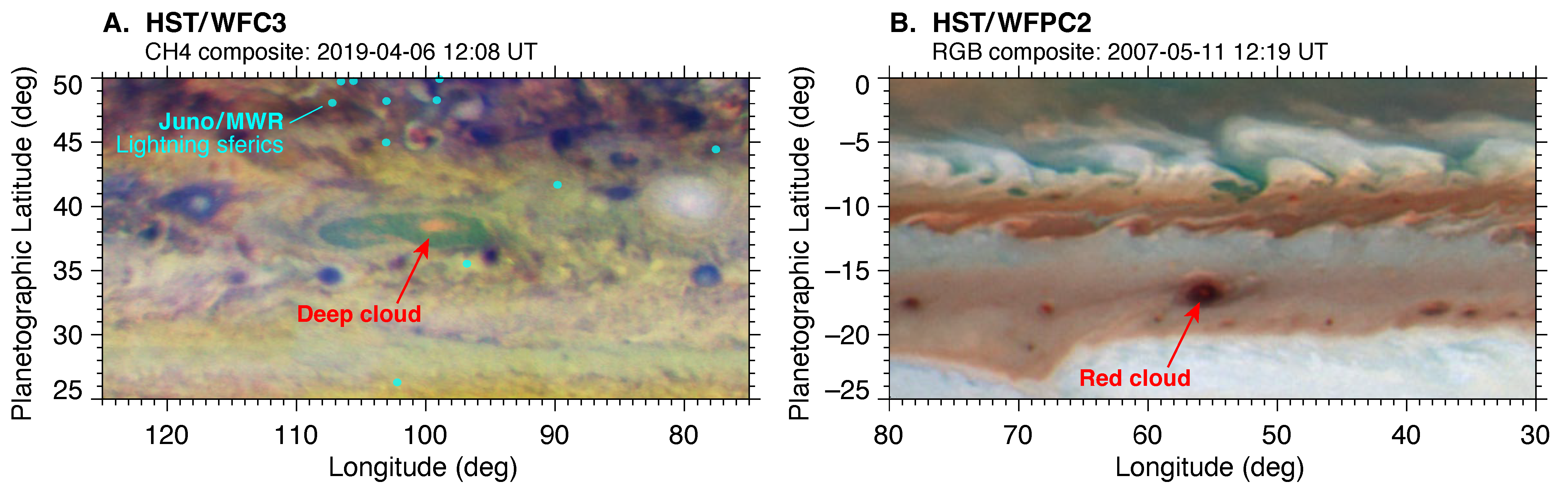
  • Great Red Spot. Bjoraker et al. [44] found cloud tops in the 4–6 bar range within the GRS, based on spectra with long integration times to achieve signal-to-noise ratios sufficient to measure the CH 3 D line shape through upper-layer cloud opacity τ haze 4 at 4.7 μ m. Temperatures at 500 mbar range from 133 K from TEXES at Gemini North [143] to 136 K from Cassini CIRS [144], encompassing the value of 134 K from Voyager IRIS [145].
Atmospheric temperatures in the upper troposphere are time-variable [146], but temperatures were not measured simultaneously with the deep cloud measurements in Bjoraker et al. [11], so 500-mbar temperature ranges in Table 3 span the full range bounded by three published zonal mean temperature datasets (Figure 21). These were mid-infrared temperature retrievals from Voyager IRIS measurements in 1979 [122], from Cassini CIRS measurements in 2000-2001 [122], and from the TEXES instrument mounted at the Gemini North observatory in 2017 [143]. We used the scatter between the datasets at each latitude to provide an estimate of the range of temperatures appropriate to the spectroscopically derived deep cloud tops and included ± 1 K arbitrarily-assigned measurement uncertainty to account for potential differences in calibration (about half the formal retrieval uncertainty for temperature at this level in Fletcher et al. [143]) and potential systematic errors from aerosols affecting retrievals of temperature at p > 400 mbar [72].
We can combine the cloud top pressure ranges, and the corresponding 500-mbar temperatures at the relevant latitudes, to narrow the parameter range in Figure 17 and provide narrower constraints on the atmospheric O/H abundance. Figure 22 shows the same O/H abundance curves with “cloud box” overlays corresponding to the deep cloud p top and T 500 information from Table 3.
The strictest upper limit is O/H > 0.5 × protosolar. This comes from the lower-left corners of the cloud boxes lying furthest to the right in the left panel (stable profile) of Figure 22. The lower left corners correspond to the lowest zonal mean temperatures at that latitude (from [122,143]), and the lowest p top for the feature, from the spectroscopic data [11]. Atmospheric O/H < 0.5 × protosolar would be inconsistent with the data for the cyclones (in both the NEB and the high-latitude FFRs), unless 500-mbar temperatures were significantly colder than the range of zonal mean temperatures derived to date, or cloud top pressures retrieved in [11] were biased to greater pressures than the actual cloud tops. Cyclone 500-mbar temperatures should actually be somewhat higher than their surroundings, not lower (Figure 12 in [55]), so the upper limit of O/H > 0.5 × protosolar is a robust value. In case Jupiter’s deep temperature structure is less stable and follows a wet adiabatic profile (right panel of Figure 22), the lower left corners of the cloud boxes give a lower limit of O/H > 2 × protosolar.
The Great Red Spot is an interesting case because it is a discrete feature with 500-mbar temperatures consistently in the 133–136 K range over decades of observations [143,144,145]. Since it is an anticyclone, its static stability should be weaker than the surroundings on theoretical grounds [8,131,132], placing its lapse rate closer to adiabatic (right panel of Figure 22). Cyclones, on the other hand, should have static stability stronger than their surroundings, with abundances closer to the contours in the left panel of the figure.
Following the theoretical arguments that lapse rates should be closer to adiabatic in anticyclones, and more stable than the surroundings in cyclones [7,8,131,132], we can perhaps reduce the uncertainty based on deep lapse rate (i.e., the difference between left and right panels of Figure 17 and Figure 22). Reading abundances derived from cyclones from the stable left panel, and abundances from the adiabatic right panel for the anticyclonic GRS, we find values near the centers of the cloud boxes close to the O/H 1–2 × protosolar contours. These abundances apply just to the cloud tops. Significantly deeper cloud bases, for vertically extended clouds, would require greater abundances. Additionally, if there is a deep sub-cloud gradient in water mixing ratio [37] (as has been found for ammonia [15,17,142]), the true atmospheric water abundance would be greater still.

4.3. Pressure Levels of the Upper Clouds

Equilibrium models feature a cloud condensation “dead zone” near 1 bar (Figure 16 and Figure 18). At this level, ammonia ice cannot condense because Jupiter’s observed temperatures are too warm for condensation of NH 3 in its observed atmospheric abundance (from in situ mass spectrometry and microwave remote sensing [15,16,17,18,142]). Ammonia condensation is even more impossible at 1 bar, if numerous observations of depleted ammonia (relative to the deep atmospheric abundance) at levels deeper than 1 bar are taken into account (e.g., [11,15,16,136,147,148,149]).
Pink curves in Figure 16 show the condensation efficiency of NH 4 SH as a function of pressure level, which decreases by two orders of magnitude over a vertical range of about 1/3 of a pressure scale height ( H g 30 km). Although the NH 4 SH cloud base may vary depending on temperature (as summarized in Figure 18), some 10 km above this level, cloud condensation of saturation-limited vapor is only 1% as efficient as at the equilibrium cloud base level. Although NH 4 SH condensed at deeper levels may be lofted up into the dead zone, it does not efficiently form there.

5. Discussion

Our radiative transfer analysis of HST imaging data in the 727-nm weak methane band and nearby continuum wavelengths suggests that data at these wavelengths do have sensitivity to deep clouds, even in the presence of an upper cloud/haze layer with significant opacity. However, quantitative interpretation of cloud depths is difficult based on imaging in these two filters alone, because the CM7 color ratio is also very sensitive to the opacity in the upper layer. There have been very few reports deriving the pressure levels of deep clouds from imaging. Banfield et al. [61] and West et al. [66] analyzed Galileo observations of cloud features with very high CM7 ratios in the GRS turbulent wake region, originally estimating a depth of 4 bar but revising the estimate to p top > 2.75 bar in the later work, which included careful treatment of upper-layer opacity. Deep clouds from Cassini imaging data were discussed by [62], but without assigning pressure levels. Li et al. [13] identified deep clouds (high CM7 ratio) inside 5-µm hot spots in Cassini imaging data, finding p top < 3 bar based on the gas-only opacity in the 727-nm filter. These deep clouds seen within 5-µm hot spots drifted with a fast speed of 170 m s 1 eastward, a similar wind speed found by the Galileo Probe at 3 bar [150], which Li et al. [13] used to imply a depth of 3 bar for the deep cloud. Under expected temperature conditions at the 8°N latitude of the 5-µm hot spots (Figure 22), a 3-bar cloud is too deep to be composed of NH 4 SH (Figure 18). The conclusion of Li et al. [13] that these deep clouds within hot spots must be water clouds is robust across the range of temperature constraints found in previous works.
Jupiter’s high latitudes—particularly the region north of about 45°N—are darker overall at visible/near-infrared wavelenths, and brighter at 5 µm. Belts at lower latitudes have high 5-µm emission and darker visible/near-infrared reflectance, but with a higher degree of inhomogeneity. The difference seems to be primarily an effect of reduced upper cloud/haze opacity, which is more uniform than deep cloud opacity. The reduced upper cloud/haze opacity and the increased lightning frequency found in Juno data [82,151] could be related. Lightning is a marker of moist convection, and Guillot et al. [35,37] suggested that strong moist convection may cause strong depletion of ammonia mixing ratios through mixed-phase water/ammonia condensation in “mushballs.” Increased convective activity may result in more widespread ammonia depletion, in turn reducing the efficiency of upper cloud condensation. This hypothesis is generally supported by the increased lightning frequency in belts [152] and patterns consistent with lower ammonia mixing ratio in belts relative to adjacent zones, spanning 6 bar [11] to 440 mbar [153] levels.
More accurate measurements of deep cloud pressure levels will require improvements in remote sensing data. The imaging data presented here show spatial variations down to the HST resolution limit of about 230 km. However, the analysis shows that filter imaging is not sufficient to break degeneracies between upper and lower cloud layer opacity and pressure level, and our basic analysis did not even allow other cloud properties to vary, like particle scale height, particle single scattering albedo, or ammonia volume mixing ratio (significant near 750 nm). Spectral data spanning the 727-nm methane band and nearby continuum wavelengths is needed, but at spatial resolutions that are not achievable by ground-based visble spectro-imaging systems currently in use, e.g., [84,85]. Visible-wavelength adaptive optics would enable high spatial resolution spectra, if a wide enough field of view can be corrected: Jupiter’s diameter is typically 35–50", and guide stars for wavefront sensing would cover additional area. Although analyses using limb darkening curves can make up for the lack of spectral coverage in imaging data [65,86], these approaches are difficult to apply to longitudinally variable cloud properties in compact features.
Narrowing the cloud boxes in Figure 22 would also require advances in remote sensing, permitting simultaneous measurement of cloud top pressure level and 500-mbar temperatures. The TEXES spectrometer has the capability to conduct this kind of simultaneous spectroscopic observation, if the right observing modes are selected. Anticipated radio occultation data from Juno will deliver new constraints on the temperatures above 500 mbar [154]. However, even with perfect knowledge of the 500-mbar temperature, Figure 22 shows that the uncertain deep temperature structure leads to a factor of four range in O/H abundance corresponding to a specific LCL. Future theoretical and/or observational constraints on the thermal structure at p > 500 mbar would provide the greatest advance in the ability to link p cloud and O/H.
Constraining Jupiter’s atmospheric composition—particularly its O/H ratio—is important for models of the planet’s interior structure, evolution, and formation [155,156,157,158].
The Galileo Probe Nephelometer measured an apparent thin condensation cloud with a well-defined base near 1.34 bar [133]. This mysterious cloud layer is located directly in the cloud condensation dead zone. Atreya et al. [112] explained the pressure level of this cloud layer in terms of condensation of NH 4 SH with greatly depleted local concentrations of NH 3 and H 2 S. However, Wong et al. [113] used an updated cloud density method in the ECCM to show that the observed density of the observed cloud layer is very high given the low NH 4 SH condensation efficiency described above. The observed density—if explained in terms of condensation alone—would require a huge updraft length scale of L = 10 km (Equation (3)). Retrievals based on visible and infrared spectroscopic data from Galileo NIMS, Cassini CIRS, and VLT MUSE have also found cloud opacity between 1 and 2 bar [84,159,160,161,162]. Interestingly, these retrievals share the characteristic that the aerosol models applied did not have an imposed constraint that cloud layers were located outside of the thermodynamic dead zone.
Clouds in the 1-bar dead zone suggest that our knowledge of cloud physics in the NH 3 -H 2 S system is in need of improvement. The microphysics of NH 4 SH is poorly understood; it is a precipitate of a gas-phase reaction of NH 3 and H 2 S. If this reaction is inhibited until high levels of disequilibrium (similar to supersaturation), it could be possible to achieve more efficient condensation within the dead zone found in equilibrium models. Another possibility is that other compounds are formed from the reaction of NH 3 and H 2 S [15,112,163]. Previous suggestions that ammonia hydrates NH 3 · H 2 O or 2NH 3 · H 2 O may produce tenuous clouds below the NH 3 ice cloud [155,164] were discounted by Weidenschilling and Lewis [114], and these hydrates are not included in most modern ECCM codes, particularly as updated Jovian atmospheric parameters led to lower temperatures and lower water partial pressures at this level of the atmosphere. An exception is the mushball scenario in Guillot et al. [35], where the low availability of water in the dead zone (due to saturation-limited vapor) can be overcome by advection of condensed water from below, via strong convective updrafts. Adsorption of NH 3 into the advected water aerosols [165] can then lead to build-up of NH 3 · H 2 O liquid and solid phases. Alternative chemistry in the NH 3 -H 2 S system remains an appealing hypothesis for explaining widespread cloud opacity in the 1–2 bar region, since mushball formation should be limited just to isolated areas of strong moist convection.

6. Conclusions

In Bjoraker et al. [11] and this paper, we took a detailed look at deep clouds in Jupiter’s atmosphere, with the goal of relating deep cloud levels to the O/H abundance in the atmosphere. We highlight areas where improvements in observational and theoretical data may someday help reach this goal.
The water cloud base pressure (LCL) is a function of the temperature and the O/H abundance. We examined the full range of temperature at 500 mbar (the upper boundary condition), and the range of temperature lapse rates consistent with observations and theory, and found that the large uncertainty in temperatures means that constraints on O/H from water LCL are very loose.
  • Deep cloud tops at 5–7 bar from spectroscopic data [11] provide a strict upper limit of O/H > 0.5 × protosolar. Values closer to the means (for 500-mbar temperature and cloud top pressure) correspond to O/H > 1–4 × protosolar.
  • Over the full range of temperatures considered, clouds at 3 bar or deeper in almost all cases must be water clouds (too deep to be NH 4 SH).
We analyzed HST data in continuum and weak methane band filters (including their ratio, CM7) to constrain deep clouds in the Juno era. A similar approach has been used previously with data from Galileo and Cassini. We used the SUNBEAR code to perform forward model calculations to identify conditions under which meaningful constraints on deep clouds could be placed.
  • A layer of cloud and haze in an upper layer (p < 1 bar) has a strong effect on CM7 and filter reflectivities. This upper layer had τ 3 over all locations in a full-disk image of Jupiter.
  • No results from 727-nm and continuum filter reflectivities alone can conclusively determine deep cloud levels, because changes in the opacity of the upper layer are degenerate with properties of the deep cloud layer.
We used CH 4 -band composite maps to show deep clouds in different contexts around the planet:
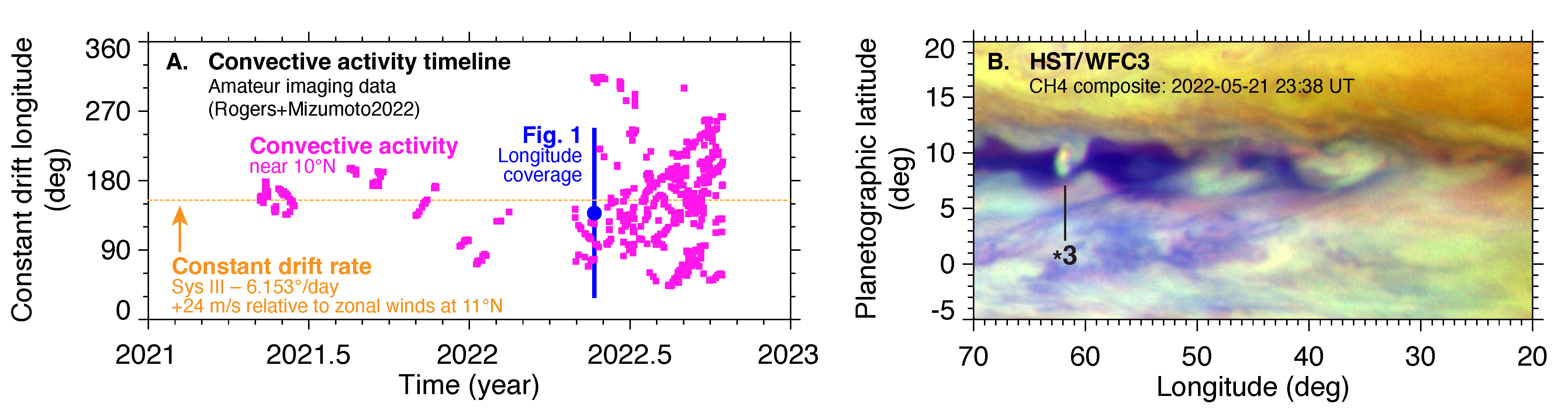
  • During the 2021–2022 period, convective activity in the NEB first shut off, then resumed at a single “stealth superstorm” longitude that drifted around the planet at a constant speed (about 6.153 °/day in System III). Activity at the stealth superstorm longitude had both similarities and differences to large convective superstorms seen on Jupiter and Saturn: it continued for many months and drifted at a constant speed like a superstorm, but it had modest vertical extent and did not always show the three-component cloud structure consistent with active moist convection.
  • We identified a region north of 45°N seen to have unique cloud structure at several epochs within the Juno era, although a full time-series analysis was not performed. The region has elevated and roughly uniform/homogeneous 5-µm brightness compared to other regions, and it is darker at visible/near-infrared wavelengths, with a high CM7 ratio. A PCA analysis supports the interpretation that this region has reduced upper cloud/haze opacity, but similar deep cloud opacity and distribution as at other latitudes. The same region has enhanced lightning frequency in Juno data [82,151].
  • Deep clouds are sometimes seen without evidence of active moist convection. In some cases, these deep clouds may precede convective outbreaks or persist after them. Compact central clouds can sometimes be seen within non-convecting cyclonic vortices (i.e., vortices without turbulent filamentary cloud structure or intense lightning activity).
The understanding of deep clouds on Jupiter—and their implications for the convective process and the atmospheric O/H abundance—could be advanced by improvements in remote sensing data:
  • Future work to determine the pressure level of deep clouds from imaging data in the weak methane band would benefit from simultaneous spectroscopy to characterize the vertical distribution of opacity over multiple levels. However, current ground-based spectroscopic instrumentation in the 600–900 nm range is seeing-limited, without the ability to resolve features at the 260 km scales detectable with HST. Full-disk spectroscopic observations at HST spatial resolution is not yet technologically feasible, but advances in adaptive optics could eventually lead to a better understanding of deep clouds on Jupiter.
  • Much tighter O/H constraints in the future could be achieved by combining high-resolution spectra at 5 μ m to measure deep cloud top levels, with simultaneous resolved mid-infrared temperature retrievals. This is technologically feasible with instrumentation such as TEXES, although such an effort would benefit from simultaneous imaging at higher spatial resolution to characterize the effects of horizontal inhomogeneity.
  • The current uncertainty in the deep lapse rate (between 500 mbar and the water cloud base) leads to an uncertainty with a factor of about four in the O/H abundance derived from water cloud pressure levels, even in best-case scenarios when simultaneous infrared deep cloud level and 500-mbar temperature retrievals are both available. There is currently no clear pathway toward better observational constraints on the deep lapse rate, but improvements in analysis of existing data and theoretical models might lead to the next advance. In particular, submillimeter and microwave observations are sensitive to temperature as well as composition (mainly ammonia), so efforts to somehow disentangle these degenerate properties would have high potential value.

Supplementary Materials

Three bundles of supporting information can be downloaded at: https://www.mdpi.com/article/10.3390/rs15030702/s1. SM1 contains supplemental figures, captions, and a table provided in a single PDF file, including Figures S01–S12 and Table S1 (enlargements and different views of panels from Figure 1, with specific features marked and discussed in the table); Figures S13–S17 (showing the reflectivity in HST/WFC3 filters as a function of μ 0 for all model aerosol structures tested, following the format of Figure 12); and Figures S18–S22 (showing CM7 ratios as a function of μ 0 for all model aerosol structures tested, following the format of Figure 14). SM2 contains multi-extension FITS files with modeled reflectivities in HST/WFC3 filters F631N, FQ727N, and FQ750N, calculated over the geometrical grids shown in Figure 10; and Jupyter Notebook documents containing Python commands used to generate figures based on the SM2 FITS files. SM3 contains a set of individual ECCM model runs stored as text files, which were used to construct the contours and curves in Figure 16, Figure 17 and Figure 18 and Figure 22; and Jupyter Notebook documents containing Python commands used to generate figures based on the SM3 text files. Jupyter Notebooks and Python code are not supported or guaranteed to run on any machine, but the commands (and saved output) are useful for interpreting the data structure of the supplementary files.

Author Contributions

Conceptualization and formulation, M.H.W., G.L.B. and S.K.A.; methodology, data curation, writing—original draft preparation, M.H.W.; visualization, M.H.W. and S.H.L.-C.; telescope data processing and acquisition, M.H.W., A.W.S. and I.d.P.; funding acquisition, M.H.W., G.L.B. and I.d.P.; radiative transfer code development, validation, and implementation, C.G., S.H.L.-C., M.H.W. and I.d.P.; equilibrium cloud condensation code supervision, development, and implementation, S.K.A. and M.H.W.; Juno MWR lightning detections and mapping, S.T.B. and M.H.W.; writing—review and editing, M.H.W., S.H.L.-C., I.d.P., G.L.B. and S.K.A. All authors have read and agreed to the published version of the manuscript.

Funding

STScI is operated by the Association of Universities for Research in Astronomy, Inc. (AURA), under NASA contract NAS5-26555. The international Gemini Observatory is a program of NSF’s NOIRLab, managed by AURA under a cooperative agreement with NSF on behalf of the Gemini Observatory partnership: the National Science Foundation (NSF, United States), National Research Council (Canada), Agencia Nacional de Investigación y Desarrollo (Chile), Ministerio de Ciencia, Tecnología e Innovación (Argentina), Ministério da Ciência, Tecnologia, Inovações e Comunicações (Brazil), and Korea Astronomy and Space Science Institute (Republic of Korea). The authors acknowledge support from STScI for programs GO-10782, GO-14661, GO-16074, and GO-16913; from the NASA Solar System Observations program through grants and cooperative agreement 80NSSC21M0344, 80NSSC18K1001, and 80NSSC19M0189; from the NASA Juno Participating Scientist program for proposals 17-JUNOPS17_2-0048 (grant 80NSSC19K1265) and 17-JUNOPS17_2-0031; and from the international Gemini Observatory.

Data Availability Statement

Based on observations made with the NASA/ESA Hubble Space Telescope, obtained at STScI. These observations are associated with programs listed in Table 1. HST data in raw form can be obtained by searching these program numbers in MAST at https://archive.stsci.edu/. Based on observations obtained at the international Gemini Observatory, which can be obtained in raw form by searching program numbers GN-2019A-Q-202, GN-2020B-Q-101, and GN-2021B-Q-110 in the Gemini Archive at https://archive.gemini.edu/. Hubble WFC3 and Gemini NIRI data in reduced form are available as part of the Wide Field Coverage for Juno high-level science products page at the MAST archive, which can be accessed at https://doi.org/10.17909/T94T1H.

Acknowledgments

This work was enabled by the location of the Gemini North telescope within the Maunakea Science Reserve, adjacent to the summit of Maunakea. We are grateful for the privilege of observing Ka ̀āwela (Jupiter) from a place that is unique in both its astronomical quality and its cultural significance. The authors thank Joshua W. Tollefson for assistance with initial setup of the SUNBEAR code, Shinji Mizumoto for sharing the cloud tracking data in Figure 4A in numerical form, Paul N. Romani for discussion of updated protosolar abundance tabulations and for their contributions to the ECCM (along with Joong Hyun In who ported it to C and added cloud condensation efficiency from Equation 3, Glenn S. Orton for his role in motivating the NIRI imaging campaigns in the Juno era, Steven M. Levin for a JPL Astrophysics Colloquium invitation that inspired some of the work on the high-latitude region north of 45°N, and the STScI Office of Public Outreach for generating the schematic shown in Figure 2c. The research was conducted with the assistance of several open-source and publicly available tools: the Astrophysics Data System, JPL Horizons, the SAO DS9 FITS viewer, the dfits and fitsort FITS header tools from ESO, Python, and the Python packages Astropy, Numpy, Matplotlib, and Scipy.

Conflicts of Interest

The authors declare no conflict of interest.

Abbreviations

The following abbreviations are used in this manuscript:
AURAAssociation of Universities for Research in Astronomy, Inc.
CAPEConvective available potential energy
CINConvective inhibition
CIRSComposite InfraRed Spectrometer
CM7Continuum to methane (727-nm) reflectivity ratio
ECCMEquilibrium cloud condensation model
ESAEuropean Space Administration
ESOEuropean Southern Observatory
EZEquatorial Zone, 7.2°S–6.9°N [123]
FFRFolded filamentary region (convectively-active cyclonic vortex)
FITSFlexible Image Transport System (binary data format)
GRSGreat Red Spot
HSTHubble Space Telescope
JIRAMJuno InfraRed Auroral Mapper
JPLJet Propulsion Laboratory
LCLLifting condensation level (cloud base)
MASTMikulski Archive for Space Telescopes
MUSEMulti Unit Spectroscopic Explorer
MWRJuno Microwave Radiometer
NASANational Aeronautic and Space Administration
NEBNorth Equatorial Belt, 6.9°N–17.4°N [123]
NIMSNear Infrared Mapping Spectrometer
NIRINear InfraRed Imager
NOIRLabNational Optical Infrared Laboratory
NSFNational Science Foundation
PCPrincipal component
PCAPrincipal components analysis
PJPerijove (Jupiter periapsis)
RGBRed, green, and blue
SAOSmithsonian Astrophysical Observatory
SEBSouth Equatorial Belt, 19.7°S–7.2°S [123]
SMSupplemental Materials
STScISpace Telescope Science Institute
TEXESTexas Echelon Cross Echelle Spectrograph
UTUniversal Time
VLTVery Large Telescope
WFC3Wide Field Camera 3
WFPC2Wide-Field and Planetary Camera 2

References

  1. West, R.A.; Strobel, D.F.; Tomasko, M.G. Clouds, aerosols, and photochemistry in the Jovian atmosphere. Icarus 1986, 65, 161–217. [Google Scholar] [CrossRef]
  2. Karkoschka, E.; Tomasko, M.G. The haze and methane distributions on Neptune from HST-STIS spectroscopy. Icarus 2011, 211, 780–797. [Google Scholar] [CrossRef]
  3. Karkoschka, E. Neptune’s cloud and haze variations 1994-2008 from 500 HST-WFPC2 images. Icarus 2011, 215, 759–773. [Google Scholar] [CrossRef]
  4. Luszcz-Cook, S.H.; de Kleer, K.; de Pater, I.; Adamkovics, M.; Hammel, H.B. Retrieving Neptune’s aerosol properties from Keck OSIRIS observations. I. Dark regions. Icarus 2016, 276, 52–87. [Google Scholar] [CrossRef] [Green Version]
  5. Irwin, P.G.J.; Teanby, N.A.; Fletcher, L.N.; Toledo, D.; Orton, G.S.; Wong, M.H.; Roman, M.T.; Pérez-Hoyos, S.; James, A.; Dobinson, J. Hazy Blue Worlds: A Holistic Aerosol Model for Uranus and Neptune, Including Dark Spots. J. Geophys. Res. Planets 2022, 127, e07189. [Google Scholar] [CrossRef] [PubMed]
  6. Atreya, S.K.; Wong, A.S.; Baines, K.H.; Wong, M.H.; Owen, T.C. Jupiter’s ammonia clouds—Localized or ubiquitous? Planet. Space Sci. 2005, 53, 498–507. [Google Scholar] [CrossRef] [Green Version]
  7. Wong, M.H.; de Pater, I.; Asay-Davis, X.; Marcus, P.S.; Go, C.Y. Vertical structure of Jupiter’s Oval BA before and after it reddened: What changed? Icarus 2011, 215, 211–225. [Google Scholar] [CrossRef]
  8. Marcus, P.S.; Pei, S.; Jiang, C.H.; Hassanzadeh, P. Three-Dimensional Vortices Generated by Self-Replication in Stably Stratified Rotating Shear Flows. Phys. Rev. Lett. 2013, 111, 084501. [Google Scholar] [CrossRef] [Green Version]
  9. de Pater, I.; Fletcher, L.N.; Luszcz-Cook, S.; DeBoer, D.; Butler, B.; Hammel, H.B.; Sitko, M.L.; Orton, G.; Marcus, P.S. Neptune’s global circulation deduced from multi-wavelength observations. Icarus 2014, 237, 211–238. [Google Scholar] [CrossRef]
  10. Tollefson, J.; Pater, I.d.; Marcus, P.S.; Luszcz-Cook, S.; Sromovsky, L.A.; Fry, P.M.; Fletcher, L.N.; Wong, M.H. Vertical wind shear in Neptune’s upper atmosphere explained with a modified thermal wind equation. Icarus 2018, 311, 317–339. [Google Scholar] [CrossRef]
  11. Bjoraker, G.L.; Wong, M.H.; de Pater, I.; Hewagama, T.; Ádámkovics, M. The Spatial Variation of Water Clouds, NH3, and H2O on Jupiter Using Keck Data at 5 microns. Remote Sens. 2022, 14, 4567. [Google Scholar] [CrossRef]
  12. Gao, P.; Wakeford, H.R.; Moran, S.E.; Parmentier, V. Aerosols in Exoplanet Atmospheres. J. Geophys. Res. Planets 2021, 126, e06655. [Google Scholar] [CrossRef]
  13. Li, L.; Ingersoll, A.P.; Vasavada, A.R.; Simon-Miller, A.A.; Del Genio, A.D.; Ewald, S.P.; Porco, C.C.; West, R.A. Vertical wind shear on Jupiter from Cassini images. J. Geophys. Res. Planets 2006, 111, E04004. [Google Scholar] [CrossRef]
  14. Sromovsky, L.A.; Baines, K.H.; Fry, P.M.; Carlson, R.W. A possibly universal red chromophore for modeling color variations on Jupiter. Icarus 2017, 291, 232–244. [Google Scholar] [CrossRef] [Green Version]
  15. de Pater, I.; Dunn, D.; Romani, P.; Zahnle, K. Reconciling Galileo Probe Data and Ground-Based Radio Observations of Ammonia on Jupiter. Icarus 2001, 149, 66–78. [Google Scholar] [CrossRef]
  16. Wong, M.H.; Mahaffy, P.R.; Atreya, S.K.; Niemann, H.B.; Owen, T.C. Updated Galileo probe mass spectrometer measurements of carbon, oxygen, nitrogen, and sulfur on Jupiter. Icarus 2004, 171, 153–170. [Google Scholar] [CrossRef]
  17. Li, C.; Ingersoll, A.; Janssen, M.; Levin, S.; Bolton, S.; Adumitroaie, V.; Allison, M.; Arballo, J.; Bellotti, A.; Brown, S.; et al. The distribution of ammonia on Jupiter from a preliminary inversion of Juno microwave radiometer data. Geophys. Res. Lett. 2017, 44, 5317–5325. [Google Scholar] [CrossRef] [Green Version]
  18. Li, C.; Ingersoll, A.; Bolton, S.; Levin, S.; Janssen, M.; Atreya, S.; Lunine, J.; Steffes, P.; Brown, S.; Guillot, T.; et al. The water abundance in Jupiter’s equatorial zone. Nat. Astron. 2020, 4, 609–616. [Google Scholar] [CrossRef] [Green Version]
  19. Asplund, M.; Grevesse, N.; Sauval, A.J.; Scott, P. The Chemical Composition of the Sun. Annu. Rev. Astron. Astrophys. 2009, 47, 481–522. [Google Scholar] [CrossRef] [Green Version]
  20. Asplund, M.; Amarsi, A.M.; Grevesse, N. The chemical make-up of the Sun: A 2020 vision. Astron. Astrophys. 2021, 653, A141. [Google Scholar] [CrossRef]
  21. Turcotte, S.; Wimmer-Schweingruber, R.F. Possible in situ tests of the evolution of elemental and isotopic abundances in the solar convection zone. J. Geophys. Res. Space Phys. 2002, 107, 1442. [Google Scholar] [CrossRef] [Green Version]
  22. Vinyoles, N.; Serenelli, A.M.; Villante, F.L.; Basu, S.; Bergström, J.; Gonzalez-Garcia, M.C.; Maltoni, M.; Peña-Garay, C.; Song, N. A New Generation of Standard Solar Models. Astrophys. J. 2017, 835, 202. [Google Scholar] [CrossRef] [Green Version]
  23. Niemann, H.B.; Atreya, S.K.; Carignan, G.R.; Donahue, T.M.; Haberman, J.A.; Harpold, D.N.; Hartle, R.E.; Hunten, D.M.; Kasprzak, W.T.; Mahaffy, P.R.; et al. The composition of the Jovian atmosphere as determined by the Galileo probe mass spectrometer. J. Geophys. Res. 1998, 103, 22831–22846. [Google Scholar] [CrossRef]
  24. Showman, A.P.; Dowling, T.E. Nonlinear Simulations of Jupiter’s 5-Micron Hot Spots. Science 2000, 289, 1737–1740. [Google Scholar] [CrossRef] [PubMed]
  25. Friedson, A.J. Water, ammonia, and H2S mixing ratios in Jupiter’s five-micron hot spots: A dynamical model. Icarus 2005, 177, 1–17. [Google Scholar] [CrossRef]
  26. Janssen, M.A.; Oswald, J.E.; Brown, S.T.; Gulkis, S.; Levin, S.M.; Bolton, S.J.; Allison, M.D.; Atreya, S.K.; Gautier, D.; Ingersoll, A.P.; et al. MWR: Microwave Radiometer for the Juno Mission to Jupiter. Space Sci. Rev. 2017, 213, 139–185. [Google Scholar] [CrossRef]
  27. Bolton, S.J.; Adriani, A.; Adumitroaie, V.; Allison, M.; Anderson, J.; Atreya, S.; Bloxham, J.; Brown, S.; Connerney, J.E.P.; DeJong, E.; et al. Jupiter’s interior and deep atmosphere: The initial pole-to-pole passes with the Juno spacecraft. Science 2017, 356, 821–825. [Google Scholar] [CrossRef] [Green Version]
  28. Li, C.; Allison, M.; Atreya, S.; Bhattacharya, A.; Fletcher, L.; Galanti, E.; Guillot, T.; Ingersoll, I.; Kaspi, Y.; Li, L.; et al. Jupiter’s tropospheric temperature and composition revealed by the Juno Microwave Radiometer. Nat. Astron. 2022, submitted.
  29. Steffes, P.; Bolton, S.; Levin, S. Laboratory Measurements of the Microwave Opacity of Water Vapor under Temperature Conditions Characteristic of the Deep Atmopshere of Jupiter. In Proceedings of the 44th COSPAR Scientific Assembly, Athens, Greece, 16–24 July 2022; Volume 44. Abstract Number B5.3-0028-22. Available online: https://ui.adsabs.harvard.edu/abs/2022cosp...44..550S (accessed on 19 October 2022).
  30. Dyudina, U.A.; Ingersoll, A.P.; Vasavada, A.R.; Ewald, S.P.; the Galileo SSI Team. Monte Carlo Radiative Transfer Modeling of Lightning Observed in Galileo Images of Jupiter. Icarus 2002, 160, 336–349. [Google Scholar] [CrossRef]
  31. Wong, M.H.; Lunine, J.I.; Atreya, S.K.; Johnson, T.; Mahaffy, P.R.; Owen, T.C.; Encrenaz, T. Oxygen and Other Volatiles in the Giant Planets and their Satellites. Rev. Mineral. Geochem. 2008, 68, 219–246. [Google Scholar] [CrossRef] [Green Version]
  32. Aglyamov, Y.S.; Lunine, J.; Becker, H.N.; Guillot, T.; Gibbard, S.G.; Atreya, S.; Bolton, S.J.; Levin, S.; Brown, S.T.; Wong, M.H. Lightning Generation in Moist Convective Clouds and Constraints on the Water Abundance in Jupiter. J. Geophys. Res. Planets 2021, 126, e06504. [Google Scholar] [CrossRef]
  33. Levin, Z.; Borucki, W.J.; Toon, O.B. Lightning generation in planetary atmospheres. Icarus 1983, 56, 80–115. [Google Scholar] [CrossRef]
  34. Becker, H.N.; Alexander, J.W.; Atreya, S.K.; Bolton, S.J.; Brennan, M.J.; Brown, S.T.; Guillaume, A.; Guillot, T.; Ingersoll, A.P.; Levin, S.M.; et al. Small lightning flashes from shallow electrical storms on Jupiter. Nature 2020, 584, 55–58. [Google Scholar] [CrossRef] [PubMed]
  35. Guillot, T.; Stevenson, D.J.; Atreya, S.K.; Bolton, S.J.; Becker, H.N. Storms and the Depletion of Ammonia in Jupiter: I. Microphysics of “Mushballs”. J. Geophys. Res. Planets 2020, 125, e06403. [Google Scholar] [CrossRef]
  36. Bjoraker, G.L.; Larson, H.P.; Kunde, V.G. The gas composition of Jupiter derived from 5 micron airborne spectroscopic observations. Icarus 1986, 66, 579–609. [Google Scholar] [CrossRef]
  37. Guillot, T.; Li, C.; Bolton, S.J.; Brown, S.T.; Ingersoll, A.P.; Janssen, M.A.; Levin, S.M.; Lunine, J.I.; Orton, G.S.; Steffes, P.G.; et al. Storms and the Depletion of Ammonia in Jupiter: II. Explaining the Juno Observations. J. Geophys. Res. Planets 2020, 125, e06404. [Google Scholar] [CrossRef]
  38. Fletcher, L.N.; Kaspi, Y.; Guillot, T.; Showman, A.P. How Well Do We Understand the Belt/Zone Circulation of Giant Planet Atmospheres? Space Sci. Rev. 2020, 216, 30. [Google Scholar] [CrossRef] [Green Version]
  39. Duer, K.; Gavriel, N.; Galanti, E.; Kaspi, Y.; Fletcher, L.N.; Guillot, T.; Bolton, S.J.; Levin, S.M.; Atreya, S.K.; Grassi, D.; et al. Evidence for Multiple Ferrel-Like Cells on Jupiter. Geophys. Res. Lett. 2021, 48, e95651. [Google Scholar] [CrossRef]
  40. de Pater, I.; Sault, R.J.; Moeckel, C.; Moullet, A.; Wong, M.H.; Goullaud, C.; DeBoer, D.; Butler, B.J.; Bjoraker, G.; Ádámkovics, M.; et al. First ALMA Millimeter-wavelength Maps of Jupiter, with a Multiwavelength Study of Convection. Astron. J. 2019, 158, 139. [Google Scholar] [CrossRef]
  41. Prinn, R.G.; Barshay, S.S. Carbon monoxide on Jupiter and implications for atmospheric convection. Science 1977, 198, 1031–1034. [Google Scholar] [CrossRef]
  42. Fegley, B., Jr.; Lodders, K. Chemical models of the deep atmospheres of Jupiter and Saturn. Icarus 1994, 110, 117–154. [Google Scholar] [CrossRef]
  43. Bézard, B.; Lellouch, E.; Strobel, D.; Maillard, J.P.; Drossart, P. Carbon Monoxide on Jupiter: Evidence for Both Internal and External Sources. Icarus 2002, 159, 95–111. [Google Scholar] [CrossRef]
  44. Bjoraker, G.L.; Wong, M.H.; de Pater, I.; Hewagama, T.; Ádámkovics, M.; Orton, G.S. The Gas Composition and Deep Cloud Structure of Jupiter’s Great Red Spot. Astron. J. 2018, 156, 101. [Google Scholar] [CrossRef]
  45. Visscher, C.; Moses, J.I. Quenching of Carbon Monoxide and Methane in the Atmospheres of Cool Brown Dwarfs and Hot Jupiters. Astrophys. J. 2011, 738, 72. [Google Scholar] [CrossRef] [Green Version]
  46. Venot, O.; Hébrard, E.; Agúndez, M.; Dobrijevic, M.; Selsis, F.; Hersant, F.; Iro, N.; Bounaceur, R. A chemical model for the atmosphere of hot Jupiters. Astron. Astrophys. 2012, 546, A43. [Google Scholar] [CrossRef] [Green Version]
  47. Wang, D.; Gierasch, P.J.; Lunine, J.I.; Mousis, O. New insights on Jupiter’s deep water abundance from disequilibrium species. Icarus 2015, 250, 154–164. [Google Scholar] [CrossRef] [Green Version]
  48. Wang, D.; Lunine, J.I.; Mousis, O. Modeling the disequilibrium species for Jupiter and Saturn: Implications for Juno and Saturn entry probe. Icarus 2016, 276. [Google Scholar] [CrossRef] [Green Version]
  49. Hyder, A.; Li, C.; Chanover, N. Hydrodynamical and Thermochemical Modeling of Jupiter’s Atmosphere—Constraining the Vertical Mass Transport. In Proceedings of the AGU Fall Meeting, Chicago, IL, USA, 12–16 December 2022; Abstract Number P25B-07. Available online: https://agu.confex.com/agu/fm22/meetingapp.cgi/Paper/1082358 (accessed on 19 October 2022).
  50. Dressel, L. WFC3 Instrument Handbook for Cycle 30 v. 14; Space Telescope Science Institute: Baltimore, MD, USA, 2022; Available online: https://ui.adsabs.harvard.edu/abs/2022wfci.book...14D (accessed on 19 October 2022).
  51. Lupie, O.; Hanley, C.; Nelan, J. Wide Field Camera #3 Filter Selection Process — Part II Compendium of Community Input; Instrument Science Report WFC3 2000-008; Space Telescope Science Institute: Baltimore, MD, USA, 2000; Available online: https://ui.adsabs.harvard.edu/abs/2000wfc..rept....8L (accessed on 19 October 2022).
  52. Hodapp, K.W.; Jensen, J.B.; Irwin, E.M.; Yamada, H.; Chung, R.; Fletcher, K.; Robertson, L.; Hora, J.L.; Simons, D.A.; Mays, W.; et al. The Gemini Near-Infrared Imager (NIRI). Publ. Astron. Soc. Pac. 2003, 115, 1388–1406. [Google Scholar] [CrossRef]
  53. Westphal, J.A. Observations of localised 5-micron radiation from Jupiter. Astrophys. J. 1969, 157, L63–L64. [Google Scholar] [CrossRef] [Green Version]
  54. Terrile, R.J.; Westphal, J.A. The Vertical Cloud Structure of Jupiter from 5 μm Measurements. Icarus 1977, 30, 274–281. [Google Scholar] [CrossRef]
  55. Wong, M.H.; Simon, A.A.; Tollefson, J.W.; de Pater, I.; Barnett, M.N.; Hsu, A.I.; Stephens, A.W.; Orton, G.S.; Fleming, S.W.; Goullaud, C.; et al. High-resolution UV/Optical/IR Imaging of Jupiter in 2016-2019. Astrophys. J. Suppl. Ser. 2020, 247, 58. [Google Scholar] [CrossRef]
  56. Imai, M.; Wong, M.H.; Kolmašová, I.; Brown, S.T.; Santolík, O.; Kurth, W.S.; Hospodarsky, G.B.; Bolton, S.J.; Levin, S.M. High-Spatiotemporal Resolution Observations of Jupiter Lightning-Induced Radio Pulses Associated With Sferics and Thunderstorms. Geophys. Res. Lett. 2020, 47, e88397. [Google Scholar] [CrossRef]
  57. Bolton, S.J.; Levin, S.M.; Guillot, T.; Li, C.; Kaspi, Y.; Orton, G.; Wong, M.H.; Oyafuso, F.; Allison, M.; Arballo, J.; et al. Microwave observations reveal the deep extent and structure of Jupiter’s atmospheric vortices. Science 2021, 374, 968–972. [Google Scholar] [CrossRef] [PubMed]
  58. Wong, M.H. Fringing in the WFC3/UVIS detector. In 2010 STScI Calibration Workshop: Hubble after SM4. Preparing JWST; Deustua, S., Oliveira, C., Eds.; Space Telescope Science Institute: Baltimore, MD, USA, 2011; pp. 189–200. Available online: https://ui.adsabs.harvard.edu/abs/2010hstc.workE..22W (accessed on 19 October 2022).
  59. Calamida, A.; Mack, J.; Medina, J.; Shanahan, C.; Bajaj, V.; Deustua, S. New Time-Dependent WFC3 UVIS Inverse Sensitivities; Instrument Science Report WFC3 2021-004; Space Telescope Science Institute: Baltimore, MD, USA, 2021; Available online: https://ui.adsabs.harvard.edu/abs/2021wfc..rept....4C (accessed on 19 October 2022).
  60. Asay-Davis, X.S.; Marcus, P.S.; Wong, M.H.; de Pater, I. Jupiter’s shrinking Great Red Spot and steady Oval BA: Velocity measurements with the ‘Advection Corrected Correlation Image Velocimetry’ automated cloud-tracking method. Icarus 2009, 203, 164–188. [Google Scholar] [CrossRef]
  61. Banfield, D.; Gierasch, P.J.; Bell, M.; Ustinov, E.; Ingersoll, A.P.; Vasavada, A.R.; West, R.A.; Belton, M.J.S. Jupiter’s Cloud Structure from Galileo Imaging Data. Icarus 1998, 135, 230–250. [Google Scholar] [CrossRef]
  62. Porco, C.C.; West, R.A.; McEwen, A.; Del Genio, A.D.; Ingersoll, A.P.; Thomas, P.; Squyres, S.; Dones, L.; Murray, C.D.; Johnson, T.V.; et al. Cassini Imaging of Jupiter’s Atmosphere, Satellites, and Rings. Science 2003, 299, 1541–1547. [Google Scholar] [CrossRef] [Green Version]
  63. Gierasch, P.J.; Ingersoll, A.P.; Banfield, D.; Ewald, S.P.; Helfenstein, P.; Simon-Miller, A.; Vasavada, A.; Breneman, H.H.; Senske, D.A.; Galileo Imaging Team. Observation of moist convection in Jupiter’s atmosphere. Nature 2000, 403, 628–630. [Google Scholar] [CrossRef] [PubMed]
  64. Sayanagi, K.M.; Dyudina, U.A.; Ewald, S.P.; Fischer, G.; Ingersoll, A.P.; Kurth, W.S.; Muro, G.D.; Porco, C.C.; West, R.A. Dynamics of Saturn’s great storm of 2010-2011 from Cassini ISS and RPWS. Icarus 2013, 223, 460–478. [Google Scholar] [CrossRef] [Green Version]
  65. Fry, P.M.; Sromovsky, L.A. Investigating temporal changes in Jupiter’s aerosol structure with rotationally-averaged 2015–2020 HST WFC3 images. Icarus 2023, 389, 115224. [Google Scholar] [CrossRef]
  66. West, R.A.; Baines, K.H.; Friedson, A.J.; Banfield, D.; Ragent, B.; Taylor, F.W. Jovian clouds and haze. In Jupiter. The Planet, Satellites and Magnetosphere; Bagenal, F., Dowling, T.E., McKinnon, W.B., Eds.; Cambridge University Press: New York, NY, USA, 2004; pp. 79–104. [Google Scholar]
  67. Little, B.; Anger, C.D.; Ingersoll, A.P.; Vasavada, A.R.; Senske, D.A.; Breneman, H.H.; Borucki, W.J.; The Galileo SSI Team. Galileo Images of Lightning on Jupiter. Icarus 1999, 142, 306–323. [Google Scholar] [CrossRef]
  68. Simon, A.A.; Wong, M.H.; Orton, G.S. First Results from the Hubble OPAL Program: Jupiter in 2015. Astrophys. J. 2015, 812, 55. [Google Scholar] [CrossRef] [Green Version]
  69. Sánchez-Lavega, A.; Rogers, J.H.; Orton, G.S.; García-Melendo, E.; Legarreta, J.; Colas, F.; Dauvergne, J.L.; Hueso, R.; Rojas, J.F.; Pérez-Hoyos, S.; et al. A planetary-scale disturbance in the most intense Jovian atmospheric jet from JunoCam and ground-based observations. Geophys. Res. Lett. 2017, 44, 4679–4686. [Google Scholar] [CrossRef] [Green Version]
  70. Rogers, J.; Mizumoto, S. Jupiter in 2022/23: Report no.2. British Astronomical Association 2022. Available online: https://britastro.org/section_information_/jupiter--section--overview/jupiter--in--2022--23/jupiter--in--2022--23--report--no--2 (accessed on 11 January 2022).
  71. Brueshaber, S. Multi-Instrument Observations of a Jovian Thunderstorm from Juno and Ground-Based Telescopes. In Proceedings of the EGU General Assembly, Vienna, Austria, 23–27 May 2022. Abstract Number EGU22-10499. [Google Scholar] [CrossRef]
  72. Beebe, R.F.; Orton, G.S.; West, R.A. Time-Variable Nature of the Jovian Cloud Properties and Thermal Structure: An Observational Perspective. In Proceedings of the Workshop on Time-Variable Phenomena in the Jovian System, Flagstaff, AZ, USA, 25–27 August 1987; NASA Special Publication 494. Belton, M.J.S., West, R.A., Rahe, J., Eds.; NASA: Washington, DC, USA, 1989; pp. 245–288. Available online: https://ntrs.nasa.gov/citations/19890019103 (accessed on 19 October 2022).
  73. Smith, B.A.; Soderblom, L.A.; Beebe, R.; Boyce, J.; Briggs, G.; Carr, M.; Collins, S.A.; Cook, A.F.I.; Danielson, G.E.; Davies, M.E.; et al. The Galilean Satellites and Jupiter: Voyager 2 Imaging Science Results. Science 1979, 206, 927–950. [Google Scholar] [CrossRef] [PubMed]
  74. Simon, A.A.; Wong, M.H.; Sromovsky, L.A.; Fletcher, L.N.; Fry, P.M. Giant Planet Atmospheres: Dynamics and Variability from UV to Near-IR Hubble and Adaptive Optics Imaging. Remote Sens. 2022, 14, 1518. [Google Scholar] [CrossRef]
  75. Dowling, T.E. Dynamics of jovian atmospheres. Annu. Rev. Fluid Mech. 1995, 27, 293–334. [Google Scholar] [CrossRef]
  76. Iñurrigarro, P.; Hueso, R.; Legarreta, J.; Sánchez-Lavega, A.; Eichstädt, G.; Rogers, J.H.; Orton, G.S.; Hansen, C.J.; Pérez-Hoyos, S.; Rojas, J.F.; et al. Observations and numerical modelling of a convective disturbance in a large-scale cyclone in Jupiter’s South Temperate Belt. Icarus 2020, 336, 113475. [Google Scholar] [CrossRef] [Green Version]
  77. Hueso, R.; Iñurrigarro, P.; Sánchez-Lavega, A.; Foster, C.R.; Rogers, J.H.; Orton, G.S.; Hansen, C.; Eichstädt, G.; Ordonez-Etxeberria, I.; Rojas, J.F.; et al. Convective storms in closed cyclones in Jupiter’s South Temperate Belt: (I) observations. Icarus 2022, 380, 114994. [Google Scholar] [CrossRef]
  78. Palotai, C.; Brueshaber, S.; Sankar, R.; Sayanagi, K. Moist Convection in the Giant Planet Atmospheres. Remote Sens. 2023, 15, 219. [Google Scholar] [CrossRef]
  79. Go, C.; de Pater, I.; Rogers, J.; Orton, G.; Marcus, P.; Wong, M.H.; Yanamandra-Fischer, P.A.; Joels, J. The Global Upheaval of Jupiter. In Proceedings of the AAS/Division for Planetary Sciences Meeting, Orlando, FL, USA, 8–12 October 2007; Volume 39. Abstract Number 19.09. Available online: https://ui.adsabs.harvard.edu/abs/2007DPS....39.1909G (accessed on 19 October 2022).
  80. Sankar, R.; Palotai, C. A new convective parameterization applied to Jupiter: Implications for water abundance near the 24°N region. Icarus 2022, 380, 114973. [Google Scholar] [CrossRef]
  81. Foster, C.; Rogers, J.; Mizumoto, S.; Orton, G.; Hansen, C.; Momary, T.; Casely, A. A rare methane-bright outbreak in Jupiter’s South Temperate domain. In Proceedings of the Europlanet Science Congress, Online, 21 September–9 October 2020. Abstract Number EPSC2020-196. [Google Scholar] [CrossRef]
  82. Brown, S.; Janssen, M.; Adumitroaie, V.; Atreya, S.; Bolton, S.; Gulkis, S.; Ingersoll, A.; Levin, S.; Li, C.; Li, L.; et al. Prevalent lightning sferics at 600 megahertz near Jupiter’s poles. Nature 2018, 558, 87–90. [Google Scholar] [CrossRef]
  83. Adriani, A.; Filacchione, G.; Di Iorio, T.; Turrini, D.; Noschese, R.; Cicchetti, A.; Grassi, D.; Mura, A.; Sindoni, G.; Zambelli, M.; et al. JIRAM, the Jovian Infrared Auroral Mapper. Space Sci. Rev. 2017, 213, 393–446. [Google Scholar] [CrossRef]
  84. Braude, A.S.; Irwin, P.G.J.; Orton, G.S.; Fletcher, L.N. Colour and tropospheric cloud structure of Jupiter from MUSE/VLT: Retrieving a universal chromophore. Icarus 2020, 338, 113589. [Google Scholar] [CrossRef] [Green Version]
  85. Dahl, E.K.; Chanover, N.J.; Orton, G.S.; Baines, K.H.; Sinclair, J.A.; Voelz, D.G.; Wijerathna, E.A.; Strycker, P.D.; Irwin, P.G.J. Vertical Structure and Color of Jovian Latitudinal Cloud Bands during the Juno Era. Planet. Sci. J. 2021, 2, 16. [Google Scholar] [CrossRef]
  86. Pérez-Hoyos, S.; Sánchez-Lavega, A.; Sanz-Requena, J.F.; Barrado-Izagirre, N.; Carrión-González, Ó.; Anguiano-Arteaga, A.; Irwin, P.G.J.; Braude, A.S. Color and aerosol changes in Jupiter after a North Temperate Belt disturbance. Icarus 2020, 352, 114031. [Google Scholar] [CrossRef]
  87. Molter, E.; de Pater, I.; Luszcz-Cook, S.; Hueso, R.; Tollefson, J.; Alvarez, C.; Sánchez-Lavega, A.; Wong, M.H.; Hsu, A.I.; Sromovsky, L.A.; et al. Analysis of Neptune’s 2017 bright equatorial storm. Icarus 2019, 321, 324–345. [Google Scholar] [CrossRef] [Green Version]
  88. Ádámkovics, M.; Wong, M.H.; Laver, C.; de Pater, I. Widespread Morning Drizzle on Titan. Science 2007, 318, 962. [Google Scholar] [CrossRef] [Green Version]
  89. Luszcz-Cook, S.H.; de Pater, I.; Ádámkovics, M.; Hammel, H.B. Seeing double at Neptune’s south pole. Icarus 2010, 208, 938–944. [Google Scholar] [CrossRef] [Green Version]
  90. de Pater, I.; Wong, M.H.; Marcus, P.; Luszcz-Cook, S.; Ádámkovics, M.; Conrad, A.; Asay-Davis, X.; Go, C. Persistent rings in and around Jupiter’s anticyclones - Observations and theory. Icarus 2010, 210, 742–762. [Google Scholar] [CrossRef]
  91. de Kleer, K.; Luszcz-Cook, S.; de Pater, I.; Ádámkovics, M.; Hammel, H.B. Clouds and aerosols on Uranus: Radiative transfer modeling of spatially-resolved near-infrared Keck spectra. Icarus 2015, 256, 120–137. [Google Scholar] [CrossRef]
  92. Ádámkovics, M.; Mitchell, J.L.; Hayes, A.G.; Rojo, P.M.; Corlies, P.; Barnes, J.W.; Ivanov, V.D.; Brown, R.H.; Baines, K.H.; Buratti, B.J.; et al. Meridional variation in tropospheric methane on Titan observed with AO spectroscopy at Keck and VLT. Icarus 2016, 270, 376–388. [Google Scholar] [CrossRef] [Green Version]
  93. Stamnes, K.; Tsay, S.C.; Jayaweera, K.; Wiscombe, W. Numerically stable algorithm for discrete-ordinate-method radiative transfer in multiple scattering and emitting layered media. Appl. Opt. 1988, 27, 2502–2509. [Google Scholar] [CrossRef] [PubMed]
  94. McCartney, E.J. Optics of the Atmosphere. Scattering by Molecules and Particles; Wiley: New York, NY, USA, 1976. [Google Scholar]
  95. Allen, C.W. Astrophysical Quantities; University of London, Athlone Press: London, UK, 1963. [Google Scholar]
  96. Sromovsky, L.A. Effects of Rayleigh-scattering polarization on reflected intensity: A fast and accurate approximation method for atmospheres with aerosols. Icarus 2005, 173, 284–294. [Google Scholar] [CrossRef]
  97. Sromovsky, L.A. Accurate and approximate calculations of Raman scattering in the atmosphere of Neptune. Icarus 2005, 173, 254–283. [Google Scholar] [CrossRef] [Green Version]
  98. Karkoschka, E. Spectrophotometry of the Jovian Planets and Titan at 300- to 1000-nm Wavelength: The Methane Spectrum. Icarus 1994, 111, 174–192. [Google Scholar] [CrossRef]
  99. Karkoschka, E. Methane, Ammonia, and Temperature Measurements of the Jovian Planets and Titan from CCD-Spectrophotometry. Icarus 1998, 133, 134–146. [Google Scholar] [CrossRef]
  100. Karkoschka, E.; Tomasko, M. The haze and methane distributions on Uranus from HST-STIS spectroscopy. Icarus 2009, 202, 287–309. [Google Scholar] [CrossRef]
  101. Lacis, A.A.; Oinas, V. A description of the correlated-k distribution method for modelling nongray gaseous absorption, thermal emission, and multiple scattering in vertically inhomogeneous atmospheres. J. Geophys. Res. 1991, 96, 9027–9064. [Google Scholar] [CrossRef] [Green Version]
  102. Karkoschka, E.; Tomasko, M.G. Methane absorption coefficients for the jovian planets from laboratory, Huygens, and HST data. Icarus 2010, 205, 674–694. [Google Scholar] [CrossRef]
  103. Irwin, P.G.J.; Bowles, N.; Braude, A.S.; Garland, R.; Calcutt, S. Analysis of gaseous ammonia (NH3) absorption in the visible spectrum of Jupiter. Icarus 2018, 302, 426–436. [Google Scholar] [CrossRef] [Green Version]
  104. Edgington, S.G.; Atreya, S.K.; Trafton, L.M.; Caldwell, J.J.; Beebe, R.F.; Simon, A.A.; West, R.A. Ammonia and Eddy Mixing Variations in the Upper Troposphere of Jupiter from HST Faint Object Spectrograph Observations. Icarus 1999, 142, 342–356. [Google Scholar] [CrossRef] [Green Version]
  105. Carlson, R.W.; Baines, K.H.; Anderson, M.S.; Filacchione, G.; Simon, A.A. Chromophores from photolyzed ammonia reacting with acetylene: Application to Jupiter’s Great Red Spot. Icarus 2016, 274, 106–115. [Google Scholar] [CrossRef]
  106. Strycker, P.D.; Chanover, N.J.; Simon-Miller, A.A.; Banfield, D.; Gierasch, P.J. Jovian chromophore characteristics from multispectral HST images. Icarus 2011, 215, 552–583. [Google Scholar] [CrossRef] [Green Version]
  107. Loeffler, M.J.; Hudson, R.L.; Chanover, N.J.; Simon, A.A. The spectrum of Jupiter’s Great Red Spot: The case for ammonium hydrosulfide (NH4SH). Icarus 2016, 271, 265–268. [Google Scholar] [CrossRef]
  108. Tejfel’, V.G. Molecular absorption and the possible structure of the cloud layers of Jupiter and Saturn. J. Atmos. Sci. 1969, 26, 854–859. [Google Scholar] [CrossRef]
  109. Bergstralh, J.T. Methane Absorption in the Jovian Atmosphere. II. Absorption Line Formation. Icarus 1973, 19, 390–418. [Google Scholar] [CrossRef]
  110. Belton, M.J.S.; Klaasen, K.P.; Clary, M.C.; Anderson, J.L.; Anger, C.D.; Carr, M.H.; Chapman, C.R.; Davies, M.E.; Greeley, R.; Anderson, D.; et al. The Galileo Solid-State Imaging experiment. Space Sci. Rev. 1992, 60, 413–455. [Google Scholar] [CrossRef]
  111. Porco, C.C.; West, R.A.; Squyres, S.; McEwen, A.; Thomas, P.; Murray, C.D.; Del Genio, A.; Ingersoll, A.P.; Johnson, T.V.; Neukum, G.; et al. Cassini Imaging Science: Instrument Characteristics Furthermore, Anticipated Scientific Investigations At Saturn. Space Sci. Rev. 2004, 115, 363–497. [Google Scholar] [CrossRef]
  112. Atreya, S.K.; Wong, M.H.; Owen, T.C.; Mahaffy, P.R.; Niemann, H.B.; de Pater, I.; Drossart, P.; Encrenaz, T. A comparison of the atmospheres of Jupiter and Saturn: Deep atmospheric composition, cloud structure, vertical mixing, and origin. Planet. Space Sci. 1999, 47, 1243–1262. [Google Scholar] [CrossRef]
  113. Wong, M.H.; Atreya, S.K.; Kuhn, W.R.; Romani, P.N.; Mihalka, K.M. Fresh clouds: A parameterized updraft method for calculating cloud densities in one-dimensional models. Icarus 2015, 245, 273–281. [Google Scholar] [CrossRef]
  114. Weidenschilling, S.J.; Lewis, J.S. Atmospheric and cloud structures of the Jovian planets. Icarus 1973, 20, 465–476. [Google Scholar] [CrossRef]
  115. Atreya, S.K.; Romani, P. Photochemistry and Clouds of Jupiter, Saturn and Uranus. In Planetary Meteorology; Hunt, G.E., Ed.; Cambridge University Press: New York, NY, USA, 1985; pp. 17–68. [Google Scholar]
  116. Mousis, O.; Atkinson, D.H.; Ambrosi, R.; Atreya, S.; Banfield, D.; Barabash, S.; Blanc, M.; Cavalié, T.; Coustenis, A.; Deleuil, M.; et al. In Situ exploration of the giant planets. Exp. Astron. 2021. [Google Scholar] [CrossRef]
  117. Tollefson, J.; de Pater, I.; Molter, E.M.; Sault, R.J.; Butler, B.J.; Luszcz-Cook, S.; DeBoer, D. Neptune’s Spatial Brightness Temperature Variations from the VLA and ALMA. Planet. Sci. J. 2021, 2, 105. [Google Scholar] [CrossRef]
  118. Seiff, A.; Kirk, D.B.; Knight, T.C.D.; Young, R.E.; Mihalov, J.D.; Young, L.A.; Milos, F.S.; Schubert, G.; Blanchard, R.C.; Atkinson, D. Thermal structure of Jupiter’s atmosphere near the edge of a 5-μm hot spot in the north equatorial belt. J. Geophys. Res. 1998, 103, 22857–22890. [Google Scholar] [CrossRef]
  119. von Zahn, U.; Hunten, D.M.; Lehmacher, G. Helium in Jupiter’s atmosphere: Results from the Galileo probe helium interferometer experiment. J. Geophys. Res. 1998, 103, 22815–22830. [Google Scholar] [CrossRef]
  120. Mahaffy, P.R.; Niemann, H.B.; Alpert, A.; Atreya, S.K.; Demick, J.; Donahue, T.M.; Harpold, D.N.; Owen, T.C. Noble gas abundance and isotope ratios in the atmosphere of Jupiter from the Galileo Probe Mass Spectrometer. J. Geophys. Res. 2000, 105, 15061–15072. [Google Scholar] [CrossRef]
  121. Gupta, P.; Atreya, S.K.; Steffes, P.G.; Fletcher, L.N.; Guillot, T.; Allison, M.D.; Bolton, S.J.; Helled, R.; Levin, S.; Li, C.; et al. Jupiter’s Temperature Structure: A Reassessment of the Voyager Radio Occultation Measurements. Planet. Sci. J. 2022, 3, 159. [Google Scholar] [CrossRef]
  122. Simon-Miller, A.A.; Conrath, B.J.; Gierasch, P.J.; Orton, G.S.; Achterberg, R.K.; Flasar, F.M.; Fisher, B.M. Jupiter’s atmospheric temperatures: From Voyager IRIS to Cassini CIRS. Icarus 2006, 180, 98–112. [Google Scholar] [CrossRef] [Green Version]
  123. Fletcher, L.N.; Greathouse, T.K.; Orton, G.S.; Sinclair, J.A.; Giles, R.S.; Irwin, P.G.J.; Encrenaz, T. Mid-infrared mapping of Jupiter’s temperatures, aerosol opacity and chemical distributions with IRTF/TEXES. Icarus 2016, 278, 128–161. [Google Scholar] [CrossRef] [Green Version]
  124. Magalhães, J.A.; Seiff, A.; Young, R.E. The Stratification of Jupiter’s Troposphere at the Galileo Probe Entry Site. Icarus 2002, 158, 410–433. [Google Scholar] [CrossRef]
  125. Sugiyama, K.i.; Odaka, M.; Kuramoto, K.; Hayashi, Y.Y. Static stability of the Jovian atmospheres estimated from moist adiabatic profiles. Geophys. Res. Lett. 2006, 33, L03201. [Google Scholar] [CrossRef] [Green Version]
  126. Leconte, J.; Selsis, F.; Hersant, F.; Guillot, T. Condensation-inhibited convection in hydrogen-rich atmospheres. Stability against double-diffusive processes and thermal profiles for Jupiter, Saturn, Uranus, and Neptune. Astron. Astrophys. 2017, 598, A98. [Google Scholar] [CrossRef]
  127. Cho, J.Y.K.; de la Torre Juárez, M.; Ingersoll, A.P.; Dritschel, D.G. A high-resolution, three-dimensional model of Jupiter’s Great Red Spot. J. Geophys. Res. 2001, 106, 5099–5106. [Google Scholar] [CrossRef]
  128. Shetty, S.; Asay-Davis, X.S.; Marcus, P.S. On the Interaction of Jupiter’s Great Red Spot and Zonal Jet Streams. J. Atmos. Sci. 2007, 64, 4432. [Google Scholar] [CrossRef] [Green Version]
  129. Legarreta, J.; Sánchez-Lavega, A. Vertical structure of Jupiter’s troposphere from nonlinear simulations of long-lived vortices. Icarus 2008, 196, 184–201. [Google Scholar] [CrossRef]
  130. Shetty, S.; Marcus, P.S. Changes in Jupiter’s Great Red Spot (1979-2006) and Oval BA (2000-2006). Icarus 2010, 210, 182–201. [Google Scholar] [CrossRef]
  131. Hassanzadeh, P.; Marcus, P.S.; Le Gal, P. The universal aspect ratio of vortices in rotating stratified flows: Theory and simulation. J. Fluid Mech. 2012, 706, 46–57. [Google Scholar] [CrossRef] [Green Version]
  132. Lemasquerier, D.; Facchini, G.; Favier, B.; Le Bars, M. Remote determination of the shape of Jupiter’s vortices from laboratory experiments. Nat. Phys. 2020, 16, 695–700. [Google Scholar] [CrossRef] [PubMed]
  133. Ragent, B.; Colburn, D.S.; Rages, K.A.; Knight, T.C.D.; Avrin, P.; Orton, G.S.; Yanamandra-Fisher, P.A.; Grams, G.W. The clouds of Jupiter: Results of the Galileo Jupiter mission probe nephelometer experiment. J. Geophys. Res. 1998, 103, 22891–22910. [Google Scholar] [CrossRef]
  134. Gillett, F.C.; Low, F.J.; Stein, W.A. The 2.8-14-MICRON Spectrum of Jupiter. Astrophys. J. 1969, 157, 925. [Google Scholar] [CrossRef]
  135. Owen, T.; Westphal, J.A. The Clouds of Jupiter: Observational Characteristics. Icarus 1972, 16, 392–396. [Google Scholar] [CrossRef]
  136. Bjoraker, G.L.; Wong, M.H.; de Pater, I.; Ádámkovics, M. Jupiter’s Deep Cloud Structure Revealed Using Keck Observations of Spectrally Resolved Line Shapes. Astrophys. J. 2015, 810, 122. [Google Scholar] [CrossRef] [Green Version]
  137. Simon, A.A.; Hueso, R.; Iñurrigarro, P.; Sánchez-Lavega, A.; Morales-Juberías, R.; Cosentino, R.; Fletcher, L.N.; Wong, M.H.; Hsu, A.I.; de Pater, I.; et al. A New, Long-lived, Jupiter Mesoscale Wave Observed at Visible Wavelengths. Astron. J. 2018, 156, 79. [Google Scholar] [CrossRef] [PubMed]
  138. Fletcher, L.N.; Melin, H.; Adriani, A.; Simon, A.A.; Sanchez-Lavega, A.; Donnelly, P.T.; Antuñano, A.; Orton, G.S.; Hueso, R.; Kraaikamp, E.; et al. Jupiter’s Mesoscale Waves Observed at 5 μm by Ground-based Observations and Juno JIRAM. Astron. J. 2018, 156, 67. [Google Scholar] [CrossRef] [PubMed]
  139. Showman, A.P.; Ingersoll, A.P. Interpretation of Galileo Probe Data and Implications for Jupiter’s Dry Downdrafts. Icarus 1998, 132, 205–220. [Google Scholar] [CrossRef] [Green Version]
  140. Showman, A.P.; de Pater, I. Dynamical implications of Jupiter’s tropospheric ammonia abundance. Icarus 2005, 174, 192–204. [Google Scholar] [CrossRef]
  141. Ortiz, J.L.; Orton, G.S.; Friedson, A.J.; Stewart, S.T.; Fisher, B.M.; Spencer, J.R. Evolution and persistence of 5-μm hot spots at the Galileo probe entry latitude. J. Geophys. Res. 1998, 103, 23051–23069. [Google Scholar] [CrossRef]
  142. de Pater, I.; Sault, R.J.; Wong, M.H.; Fletcher, L.N.; DeBoer, D.; Butler, B. Jupiter’s ammonia distribution derived from VLA maps at 3–37 GHz. Icarus 2019, 322, 168–191. [Google Scholar] [CrossRef] [Green Version]
  143. Fletcher, L.N.; Orton, G.S.; Greathouse, T.K.; Rogers, J.H.; Zhang, Z.; Oyafuso, F.A.; Eichstädt, G.; Melin, H.; Li, C.; Levin, S.M.; et al. Jupiter’s Equatorial Plumes and Hot Spots: Spectral Mapping from Gemini/TEXES and Juno/MWR. J. Geophys. Res. Planets 2020, 125, e06399. [Google Scholar] [CrossRef]
  144. Fletcher, L.N.; Orton, G.S.; Mousis, O.; Yanamandra-Fisher, P.; Parrish, P.D.; Irwin, P.G.J.; Fisher, B.M.; Vanzi, L.; Fujiyoshi, T.; Fuse, T.; et al. Thermal structure and composition of Jupiter’s Great Red Spot from high-resolution thermal imaging. Icarus 2010, 208, 306–328. [Google Scholar] [CrossRef]
  145. Simon-Miller, A.A.; Gierasch, P.J.; Beebe, R.F.; Conrath, B.; Flasar, F.M.; Achterberg, R.K.; the Cassini CIRS Team. New Observational Results Concerning Jupiter’s Great Red Spot. Icarus 2002, 158, 249–266. [Google Scholar] [CrossRef]
  146. Orton, G.S.; Friedson, A.J.; Yanamandra-Fisher, P.A.; Caldwell, J.; Hammel, H.B.; Baines, K.H.; Bergstralh, J.T.; Martin, T.Z.; West, R.A.; Veeder, G.J., Jr.; et al. Spatial Organization and Time Dependence of Jupiter’s Tropospheric Temperatures, 1980-1993. Science 1994, 265, 625–631. [Google Scholar] [CrossRef] [Green Version]
  147. Hanley, T.R.; Steffes, P.G.; Karpowicz, B.M. A new model of the hydrogen and helium-broadened microwave opacity of ammonia based on extensive laboratory measurements. Icarus 2009, 202, 316–335. [Google Scholar] [CrossRef]
  148. Grassi, D.; Adriani, A.; Mura, A.; Dinelli, B.M.; Sindoni, G.; Turrini, D.; Filacchione, G.; Migliorini, A.; Moriconi, M.L.; Tosi, F.; et al. Preliminary results on the composition of Jupiter’s troposphere in hot spot regions from the JIRAM/Juno instrument. Geophys. Res. Lett. 2017, 44, 4615–4624. [Google Scholar] [CrossRef]
  149. Giles, R.S.; Fletcher, L.N.; Irwin, P.G.J.; Orton, G.S.; Sinclair, J.A. Ammonia in Jupiter’s Troposphere From High-Resolution 5 μm Spectroscopy. Geophys. Res. Lett. 2017, 44, 10. [Google Scholar] [CrossRef] [Green Version]
  150. Atkinson, D.H.; Pollack, J.B.; Seiff, A. The Galileo probe Doppler wind experiment: Measurement of the deep zonal winds on Jupiter. J. Geophys. Res. 1998, 103, 22911–22928. [Google Scholar] [CrossRef]
  151. Kolmašová, I.; Imai, M.; Santolík, O.; Kurth, W.S.; Hospodarsky, G.B.; Gurnett, D.A.; Connerney, J.E.P.; Bolton, S.J. Discovery of rapid whistlers close to Jupiter implying lightning rates similar to those on Earth. Nat. Astron. 2018, 2, 544–548. [Google Scholar] [CrossRef]
  152. Vasavada, A.R.; Showman, A.P. Jovian atmospheric dynamics: An update after Galileo and Cassini. Rep. Prog. Phys. 2005, 68, 1935–1996. [Google Scholar] [CrossRef] [Green Version]
  153. Achterberg, R.K.; Conrath, B.J.; Gierasch, P.J. Cassini CIRS retrievals of ammonia in Jupiter’s upper troposphere. Icarus 2006, 182, 169–180. [Google Scholar] [CrossRef]
  154. Hodges, A.L.; Steffes, P.G.; Gladstone, R.; Folkner, W.M.; Buccino, D.; Bolton, S.J.; Levin, S. Simulations of Potential Radio Occultation Studies of Jupiter’s Atmosphere using the Juno Spacecraft. In Proceedings of the AGU Fall Meeting, Online, 1–17 December 2020; Abstract Number P012–07. Available online: https://ui.adsabs.harvard.edu/abs/2020AGUFMP012...07H (accessed on 19 October 2022).
  155. Owen, T. The Atmosphere of Jupiter. Science 1970, 167, 1675–1681. [Google Scholar] [CrossRef] [PubMed]
  156. Militzer, B.; Hubbard, W.B.; Wahl, S.; Lunine, J.I.; Galanti, E.; Kaspi, Y.; Miguel, Y.; Guillot, T.; Moore, K.M.; Parisi, M.; et al. Juno Spacecraft Measurements of Jupiter’s Gravity Imply a Dilute Core. Planet. Sci. J. 2022, 3, 185. [Google Scholar] [CrossRef]
  157. Helled, R.; Stevenson, D.J.; Lunine, J.I.; Bolton, S.J.; Nettelmann, N.; Atreya, S.; Guillot, T.; Militzer, B.; Miguel, Y.; Hubbard, W.B. Revelations on Jupiter’s formation, evolution and interior: Challenges from Juno results. Icarus 2022, 378, 114937. [Google Scholar] [CrossRef]
  158. Miguel, Y.; Bazot, M.; Guillot, T.; Howard, S.; Galanti, E.; Kaspi, Y.; Hubbard, W.B.; Militzer, B.; Helled, R.; Atreya, S.K.; et al. Jupiter’s inhomogeneous envelope. Astron. Astrophys. 2022, 662. [Google Scholar] [CrossRef]
  159. Irwin, P.G.J.; Weir, A.L.; Smith, S.E.; Taylor, F.W.; Lambert, A.L.; Calcutt, S.B.; Cameron-Smith, P.J.; Carlson, R.W.; Baines, K.; Orton, G.S.; et al. Cloud structure and atmospheric composition of Jupiter retrieved from Galileo near-infrared mapping spectrometer real-time spectra. J. Geophys. Res. Planets 1998, 103, 23001–23022. [Google Scholar] [CrossRef]
  160. Irwin, P.G.J.; Sihra, K.; Bowles, N.; Taylor, F.W.; Calcutt, S.B. Methane absorption in the atmosphere of Jupiter from 1800 to 9500 cm−1 and implications for vertical cloud structure. Icarus 2005, 176, 255–271. [Google Scholar] [CrossRef]
  161. Matcheva, K.I.; Conrath, B.J.; Gierasch, P.J.; Flasar, F.M. The cloud structure of the jovian atmosphere as seen by the Cassini/CIRS experiment. Icarus 2005, 179, 432–448. [Google Scholar] [CrossRef]
  162. Alexander, C.; Irwin, P.G.J. Predetermining Parameters of Jupiter’s Atmosphere in Order to Simplify Cloud Structure. In Proceedings of the AGU Fall Meeting, Chicago, IL, USA, 12–16 December 2022; Abstract Number P25B-02. Available online: https://agu.confex.com/agu/fm22/meetingapp.cgi/Paper/1085758 (accessed on 19 October 2022).
  163. Romani, P.N.; de Pater, I.; Dunn, D.; Zahnle, K.; Washington, B. Adsorption of Ammonia onto Ammonium Hydrosulfide Cloud Particles in Jupiter’s Atmosphere. In Proceedings of the AAS/Division for Planetary Sciences Meeting, Pasadena, CA, USA, 9–13 October 2000; Volume 32. Abstract Number 04.05. Available online: https://ui.adsabs.harvard.edu/abs/2000DPS....32.0405R (accessed on 19 October 2022).
  164. Lewis, J.S. The clouds of Jupiter and the NH3-H2O and NH 3-H 2S systems. Icarus 1969, 10, 365–378. [Google Scholar] [CrossRef]
  165. Kasper, T.; Wong, M.H.; Marschall, J.; de Pater, I.; Romani, P.N.; Kalogerakis, K.S. Uptake of ammonia gas by Jovian ices. In Proceedings of the EPSC-DPS Joint Meeting, Nantes, France, 2–7 October 2011; Abstract Number EPSC-DPS2011-352. Available online: https://ui.adsabs.harvard.edu/abs/2011epsc.conf..352K (accessed on 19 October 2022).
Figure 1. Jupiter imaging data from HST and Gemini observatories map cloud opacity in shallow and deep layers. (A) An RGB color image (631, 502, 395 nm) shows Jupiter’s familiar visible appearance. (B) A CH 4 -band depth map is composed by loading 750, 727, and 889-nm frames (continuum, weak CH 4 band, strong CH 4 band) into the RGB channels. Deep clouds appear reddish in this color scheme. Boxes outline regions enlarged in Figures 4B and 6. (C) Thermal infrared imaging near 5 μ m is very bright where there is no cloud opacity and moderately bright where upper clouds are thin but there is cloud opacity at some level at p < 6 bar [11]. Dark regions have high upper cloud opacity. (D) The continuum image is sensitive to cloud opacity across both deep and shallow cloud layers. (E) The weak methane band image is sensitive to upper cloud and haze opacity ( p < 3 bar [13]). (F) The strong CH 4 band senses aerosols above the condensation clouds at p < 0.6 bar [13]. (G) The CM7 ratio (750/727 nm ratio, Equation (1)) is sensitive to the partitioning of upper/lower opacity in multiple cloud layers (while total opacity cancels out in the ratio). High values indicate more opacity at depth, and low values indicate more opacity in the upper cloud levels.
Remotesensing 15 00702 g001
Figure 2. Cloud structure from HST imaging combined with lightning detections from Juno reveal a three-component cloud structure in regions of active moist convection: deep clouds, tall thick cloud towers, and clearings. (a) HST CH 4 -band cloud depth maps identified this three-component signature of convection at high northern latitudes in 2019. Two different Juno instruments detected lightning in this region, indicating active moist convection. (b) The CM7 ratio (Equation (1)) shows high clouds in blue and deep clouds in red. Maps in panels (a,b) have been corrected for limb darkening using a Minnaert function prior to polar projection, resulting in lower numerical values of the CM7 ratio compared to the values in Figure 1G, which have been calculated without limb-darkening corrections. Nevertheless, local trends still hold, with a high dynamic range between high and low cloud depths packed into the moist convective region. (c) A schematic diagram shows the three-component convective cloud structure. Figure adapted from Imai et al. [56] (panels (a,b)) and Hubble News Release 2020–2021 (panel (c)).
Remotesensing 15 00702 g002
Figure 3. HST observations indicate deep clouds in areas sampled by Juno/MWR (right), but Juno did not detect lightning associated with these clouds. HST imaging three days prior (left) suggests an earlier moist convective eruption that may have generated lightning activity, but the storm evolved within three days, losing the tall thick cloud towers characteristic of active convection by the time Juno flew over the area. The Juno/MWR footprint envelope on 2020-07-22 is distorted to account for advection by the zonal mean flow over the three-day interval between the HST imaging data and the Juno pass (using the 2020 zonal wind profile from OPAL program data [68]).
Remotesensing 15 00702 g003
Figure 4. Convective activity in the North Equatorial Belt (NEB) was atypical in the 2021–2022 timeframe. (A) Throughout 2021, convective activity shut off in the NEB, except for episodic eruptions near the active drifting longitude (orange dashed line). Convective activity across the NEB began to spread outward from the active longitude in late 2022. Long-term episodic eruptions at a constant drifting location are typical of large convective superstorms [40,55,69]. Pink squares indicate locations of compact bright white cloud features in color imaging data [70]; the convective activity within these compact cloud features is not well constrained. (B) The three-component cloud structure of moist convective is not clearly present at the active longitude (which is marked “*3” for ease of comparison with Figures S2, S4, S6, and S8 in SM1). Although some deep clouds are suggested by red colors in the CH 4 composite, there is not much contrast between deep clouds and tall, thick, convective towers. The cloud structure in convective regions typically includes deep clouds and tall, thick, clouds with similar size scales (Figure 1 and Figure 3), but the tall and thick clouds near the active longitude dwarf the much smaller deep clouds horizontally. Juno observations of a different individual storm plume at this active longitude six months prior detected lightning [71].
Remotesensing 15 00702 g004
Figure 5. “Barges”—cyclonic vortices with smooth, well-defined edges [72]—often are dark in color with compact central clouds. These central clouds may be examples of deep water clouds in the absence of moist convection, although such clouds might precede or follow convective outbreaks. (A) The central cloud is deep (high CM7 ratio), but not associated with a cluster of lightning sferic detections that would signify active moist convection. Some clustering of lightning signals is seen further to the north, where cloud structure is consistent with moist convective activity (see Figure 2). (B) A compact central cloud was detected within a barge-like vortex in 2007 HST imaging data. Six days later, ground-based observations detected a convective superstorm originating from this cyclone [79]. No weak methane-band imaging is available in the WFPC2 dataset, but the deep red color of this cloud is suggestive of greater depth compared to adjacent clouds.
Remotesensing 15 00702 g005
Figure 6. Two cyclonic vortices are seen in different states: C45 in a cloudy oval state appears to be non-convective, while C34 in an FFR state appears to be undergoing moist convective activity. The cyclones are numbered based on their locations between anticyclonic white ovals A3, A4, and A5, as identified by Rogers and Mizumoto [70]. (A) In RGB color, cloudy oval cyclone C45 appears white. (B) The CH 4 -band composite shows a diversity of cloud opacities and depths within C34. High-altitude haze (picked up in the 889-nm channel) is depleted. (C) The white appearance of C45 in the UV composite is another effect of depleted upper-tropospheric haze. (D) The infrared map is speckled with small clearings within C34, while in C45, a thick layer of upper-level cloud opacity uniformly attenuates outgoing thermal radiation. The central dark spot from panel C is invisible in panel D, suggesting evolution over the two days separating the HST and Gemini observations.
Remotesensing 15 00702 g006
Figure 7. Infrared imaging from the JIRAM instrument [83] on Juno shows a transition from low-latitude banded emission to a high-latitude region with elevated emission overall. The image shows JIRAM data superposed on a wireframe planetocentric coordinate grid, with the planetographic latitude of 45°N marked in cyan. Figure adapted from an animation released on the official JPL-NASA YouTube channel at https://youtu.be/i9TtSCkoERw.
Remotesensing 15 00702 g007
Figure 8. HST and Gemini observations show a transition in cloud structure north of 45°N, coinciding with lightning activity detected by Juno. (A) The continuum band image is sensitive to integrated cloud opacity throughout the vertical column. (B) The weak methane band (727 nm) senses cloud opacity integrated over p 3 bar. (C) The CM7 ratio (here, ( I / F 727 ) / ( I / F 631 ) ) has high values where aerosols are located at deep levels. The CM7 ratio is low when cloud opacity is located at a shallow level (e.g., where a convective tower is marked by a blue arrow). The CM7 ratio is primarily sensitive to cloud depth rather than cloud opacity. The color scale bar is the same as in Figure 1, except the maximum value is increased to 2.6. (D) Contrast-enhanced RGB color is compared with lightning detected from Juno. Cyan points indicate Juno/MWR boresight pointings at the times that sferics were detected. The half-power envelope for one pointing is shown (elliptical shape at lower right) as a rough measure of localization precision. (E) A CH 4 -band composite, with compact deep clouds appearing red (magenta arrows), and a tall/thick convective tower appearing white. (F) Thermal emission at 5 µm is greater north of 45°N. The infrared image was taken two days after the HST images, so sites with individual compact deep clouds in the HST data cannot be accurately linked to locations in the Gemini data. Limb darkening has been removed using Minnaert functions for HST images, and an emission-angle cosine power law for the 5-µm mosaic. The CM7 ratio was calculated using data without limb-darkening corrections.
Remotesensing 15 00702 g008
Figure 9. Our aerosol framework includes deep (2–6 bar) clouds, in addition to upper clouds and hazes (see also Table 2). The framework is similar to the cloud structure of West et al. [1,66], but agnostic as to the composition of the deep clouds. The combination of a blue-absorbing chromophore haze and a higher-opacity, conservatively-scattering cloud/haze layer beneath it follows the “crème-brûlée” framework used in several recent works [65,84,85,86]. Levels where clear gas opacity reaches unit optical depth for two-way scattering of sunlight back to the observer are shown as hatched boxes for continuum and methane-band filters, with levels from Figure 3 of Fry and Sromovsky [65] and Figure 2 of Banfield et al. [61].
Remotesensing 15 00702 g009
Figure 10. Geometrical parameter values for radiative transfer calculations. We created a 16 × 16 grid by coarsely sampling the geometry for actual HST images taken during PJ 42, matching the relevant sub-observer and sub-solar latitudes. The geometric sampling was designed to test the relative effects of emission angle cosine ( μ ), incidence angle cosine ( μ 0 ), and effective gravity ( g eff ), which varies with latitude and affects the atmospheric gas pressure scale height H g = R T / μ g eff .
Remotesensing 15 00702 g010
Figure 11. Reflectivity values (left columns) and CM7 reflectivity ratios (right columns) calculated over the coarse geometrical grid defined in Figure 10. Each row is for a different deep cloud pressure level, and all calculations are for the case of τ haze = 5 and τ cloud = 25 . Overall reflectivity and limb darkening are weaker for the 727-nm filter compared to the continuum filters, because the relative contribution from upper-tropospheric haze (lying above much of the methane absorption) is greater compared to the contribution from the tropospheric cloud decks at the stated pressure levels. CM7 ratios increase with cloud depth in most cases.
Remotesensing 15 00702 g011
Figure 12. Comparison between observations (black: I / F in 727-nm and continuum filters) and models (colors) constrain the range of aerosol opacities on Jupiter in a global sense. Observed data from Figure 1 are shown in black (solid for the mean and dashed for the minimum and maximum values) as a function of solar incidence angle cosine. Data from across the disk have been sorted only by μ 0 , ignoring latitude, longitude, and type of feature to show the full range of variation over the image. Additional panels can be viewed in Figures S13–S17. The closest match to minimum I / F on the disk (lower dashed line) is the τ haze = 1 , τ cloud = 0 case (top row) for 631 nm, and τ haze = 3 , τ cloud = 5 for 727 nm and 750 nm. Mean global values are best matched by τ haze = 5 , τ cloud = 25 (third row), and maximum reflectivities are best matched by τ haze = 10 , τ cloud = 100 (bottom row). Colors correspond to deep cloud pressure levels from 2 bar (blue) to 6 bar (orange).
Remotesensing 15 00702 g012
Figure 13. Model spectra across the bandpasses of the continuum (631 and 750 nm) and weak methane band (727 nm) filters illustrate the sensitivity to deep cloud level for a fixed upper and lower opacities ( τ haze = 5 and τ cloud = 25 ). The 631-nm filter has good continuum response (no sensitivity to deep cloud level) over most of the bandpass, with some pressure-sensitivity in the blue end due to proximity to the weak methane band at 619 nm. The 727-nm bandpass is almost insensitive to deep cloud in the core of the band, but the edges of the filter bandpass give sensitivity to deep cloud pressure level. The 750-nm filter has some sensitivity to deep cloud level, presumably due to NH 3 absorption within the bandpass, but the fractional change in I / F is lower than for 727 nm, so the CM7 ratio (with 750 nm as the continuum wavlength) still serves as an indicator of cloud depth.
Remotesensing 15 00702 g013
Figure 14. CM7 values are plotted vs. μ 0 for the same model cases as in Figure 12, for the two continuum filters. With some minor exceptions discussed in the text, most of the model results fall between the dashed lines marking the minimum and maximum values in the data from Figure 1, so the results are considered Jupiter-like. Sensitivity to deep cloud pressure levels is greater for the 631/727 ratio, perhaps because ammonia gas absorption limits the usefulness of the 750-nm filter as a continuum reference wavelength. General trends support the interpretation that low CM7 values are found where there is high opacity in the upper cloud/haze layer. Deep clouds have a limited ability to increase the CM7 ratio, compared to simply reducing the opacity in the upper haze/cloud layer.
Remotesensing 15 00702 g014
Figure 15. Both I/F and CM7 curves are shown together for a single model case ( τ haze = 3 and τ cloud = 100), to illustrate the optimal conditions for detecting variation due to the cloud pressure level. The model case is Jupiter-like because it has I / F values that fall within the observed maximum and minimum values as a function of μ 0 (dashed black lines). The low upper-layer opacity is key for sensing properties of the deeper layer, while the high deep-layer opacity maximizes the signal level in the 727-nm filter that provides depth sensitivity. Distinguishing between opacity at p cloud = 2 bar and p cloud > 2 bar is sufficient to rule out NH 4 SH composition for the deep cloud layer. This could be possible ( Δ CM7 0.4 ) in a situation where the upper cloud/haze opacity are well constrained.
Remotesensing 15 00702 g015
Figure 16. The sensitivity of cloud base pressure to volatile abundance has been widely discussed in the literature. However, water cloud base levels—for the same water abundance—also vary by a factor of two between the end-member temperature structures. For example, the water cloud base for a 10× solar H 2 O abundance is 7.5 bar for a hot end-member temperature profile (panel B) and 17 bar for a cold end-member temperature profile (panel D). For 1× solar H 2 O, the cloud base for hot and cold conditions ranges from 3.8 to 7.7 bar. The Voyager 1 radio occultation profiles [121] are shown for comparison (ingress and egress profiles overlap at this scale).
Remotesensing 15 00702 g016
Figure 17. Contours of water abundance are shown as a function of lifting condensation level (LCL) on the x-axis and temperature at the 500-mbar level on the y-axis. Two panels give end member cases for temperature profile extrapolation below the 500-mbar level: a statically stable extrapolation on the left that gives colder temperatures at deep levels, and a neutrally stable extrapolation on the right that gives warmer temperatures at deep levels. Abundances are relative to the protosolar value of H 2 O/H 2 = 1.07 × 10 3 from [19].
Remotesensing 15 00702 g017
Figure 18. Over the range of plausible Jovian thermal conditions considered in this work, upper clouds of NH 3 (gold) or NH 4 SH (blue) form only at pressures < 3.2 bar. Shaded regions are bounded by adiabatic and 90% adiabatic lapse rates. Sensitivity to lapse rate increases with pressure, due to the larger vertical distance from the 500-mbar boundary condition. The same effect can be seen in Figure 16, where slopes of contour lines grow increasingly shallow at greater pressures. Red upper tick marks show the altitude scale, which varies in each case depending on the temperatures and lapse rates tested. The horizontal red line indicates the maximum and minimum pressures for each altitude, while the box gives the interval ± 1 standard deviation. The cloud symbol shows the pressure level of a cloud detected by the Galileo Probe [133], plotted against the 500-mbar temperature in the probe site [118]. This cloud, located in a “dead zone” where NH 3 cannot condense and NH 4 SH condensation is not efficient, is discussed in Section 4.3.
Remotesensing 15 00702 g018
Figure 19. Weak methane band imaging data is sensitive to deep cloud properties, which are highly inhomogeneous on short length scales (at 50° latitude, 1° is about 1130 km in the east–west direction and 830 km in the north–south direction). (A,B) HST imaging data at continuum and weak methane-band images are shown, overlapping with the areas shown in Figure 2 and Figure 5. Most of the brightness variation in the images is due to limb darkening, a function of the emission angle and (C) the solar incidence angle. (D,E) With limb darkening corrected, variation due to inhomogeneous cloud properties is clearer. (F) The CM7 ratio is calculated from the ratio panels (A,B) (i.e., on the data with no limb darkening correction). Several areas with locally high CM7 values are labeled, each with different cloud structure as described in the text. (G,H,I) Three orthogonal principal components (PCs) describe the spatial variation in the data. The first colorbar in panels (GI) gives the magnitude of each PC over the spatial domain, and the second colorbar specifies a hypothetical direct mapping of the PCs to cloud structure properties. The cloud property ranges correspond to the ranges modeled in Section 2.3. The SUNBEAR model output was then used to reconstruct the observables as a function of the remapped PCs and the incidence angle at each map pixel. (J) The reconstructed 631-nm map is a fair match to the observed data. In particular, the barge is dark, and the fine scale structure is very similar to panel (D). The map resembles panel (D) more than panel (A) in terms of north–south gradient and absolute scale. (K) The reconstructed 727-nm map was heavily limb-darkened, so a Minnaert correction was applied in order to show detail in cloud structure. (L) The qualitative match with the observed data (panel (F)) is again good, although some differences can be seen. Importantly, the local maxima from panel (F) appear as local maxima in the reconstructed CM7 map, and the values are generally higher (greater deep/upper cloud opacity fraction) north of 45°N.
Remotesensing 15 00702 g019
Figure 20. Modulation of infrared thermal emission over the map range is well described by PCs 1 and 3, supporting the interpretation that these PCs map to upper and lower cloud opacity. (A) The Gemini/NIRI 5-µm map is fully independent of the PC maps derived only from HST data. (B) PC1 (also shown in Figure 19G) is interpreted to represent τ haze . Comparison with panel (A) supports the idea that the infrared-bright northern high latitudes are a result of about a factor of two decrease in upper cloud/haze opacity. (C) PC3 (also shown in Figure 19I) is interpreted to represent τ cloud . Low PC3 amplitude in this panel corresponds well to isolated bright features in panel (A), suggesting that the bright features indicate holes in the lower cloud layer. The results are consistent with work from more than 50 years ago, which interpreted spatial variation in 5-µm imaging observations to be a result of varying opacity in a more uniform middle cloud layer and a patchier deep cloud layer [53,54,134,135]. The correlations are weaker in the upper right corner of the map, which is at high incidence angle for the HST observations ( μ 0 < 0.5 ; Figure 19C).
Remotesensing 15 00702 g020
Figure 21. Independent measurements of the zonal-mean temperature field at the 500-mbar level show consistent trends of high temperatures over the equatorial belts, gradually decreasing poleward [122,143]. The EZ temperature was depressed in the Cassini data. Differences between the temperature profiles retrieved from Cassini and Voyager data may be from temporal variability. The Gemini temperature profile is an average of seven separate scans taken over a period of 3 nights, with the standard deviation (shaded) giving a sense of longitudinal and short-timescale temporal variability. Shaded yellow bars (with latitude ranges given) indicate locations where deep cloud tops at 5–7 bar were retrieved from 5-µm spectroscopic data [11]: high-latitude folded filamentary regions (FFRs) near 56°S and 45°N, a pair of cyclonic vortices in the NEB near 18°N, and deep clouds near 8°N associated with ammonia plumes [40] in the upwelling branch of the NEB Rossby-wave system that maintains 5-micron hotspots in the downwelling branch [25,139,140]. The full range of temperatures in each yellow bar defines the height of the “cloud boxes” defined in Figure 22.
Remotesensing 15 00702 g021
Figure 22. Water abundance as a function of LCL and 500-mbar temperature, as in Figure 17, with “cloud box” overlays for deep clouds in selected locations (see Table 3). Retrieved cloud top pressures from Bjoraker et al. [11] for four features are overlaid as grey boxes with solid lines: two folded filamentary regions (FFRs) at high latitudes, a pair of cyclonic vortices in the NEB, and deep clouds associated with Rossby plumes at the EZ/NEB boundary. The full range of temperatures at the same latitude taken from Figure 21 is given by the vertical extent of each cloud box. For the GRS (dashed grey box), cloud top pressures are from Bjoraker et al. [44] and 500-mbar temperatures are from Simon-Miller et al. [145] and Fletcher et al. [143,144]. A strict limit of O/H > 0.5 × protosolar is set by the lower left corners of the boxes located furthest to the right in the left panel. A more relaxed lower limit of O/H > 1–3 × protosolar is indicated by the centers of the cloud boxes in both panels. The range tightens to 1–2 × protosolar when taking into account theoretical arguments that temperature profiles within anticyclones should be closer to neutrally stable, while cyclones should have greater static stability [7,8,131,132]. These arguments imply that the right panel is more appropriate for the GRS and the left panel is more appropriate for the NEB cyclones and high-latitude FFRs, with 1 × protosolar water (at the cloud base level) being the likely lower limit for both cyclonic and anticyclonic vortices. Cloud top heights can only give lower limits, because p top < LCL, and the abundance constraint comes from the LCL, not the observable p top .
Remotesensing 15 00702 g022
Table 3. Details of spectroscopically detected deep cloud regions (corresponding to the yellow bars in Figure 21 and the grey boxes in Figure 22).
Feature Type p top (bar) T 500 mbar (K)Bjoraker et al. [11] Figure NumbersLatitudes
FFRs7131.7–134.2 (South), 131.5–133.9 (North)4, 6, 11, 1455°S–57°S, 42°N–48°N
NEB cyclones5–6.5133.1–140.519, 21, 23, 2417°N–19°N
Rossby plumes5.5–6.5133.0–139.120, 22, 25, 266°N–9°N
GRS4–6133.0–136.022°S
Disclaimer/Publisher’s Note: The statements, opinions and data contained in all publications are solely those of the individual author(s) and contributor(s) and not of MDPI and/or the editor(s). MDPI and/or the editor(s) disclaim responsibility for any injury to people or property resulting from any ideas, methods, instructions or products referred to in the content.

