
High-Precision Single Building Model Reconstruction Based on the Registration between OSM and DSM from Satellite Stereos
Abstract
:1. Introduction
2. Methodology
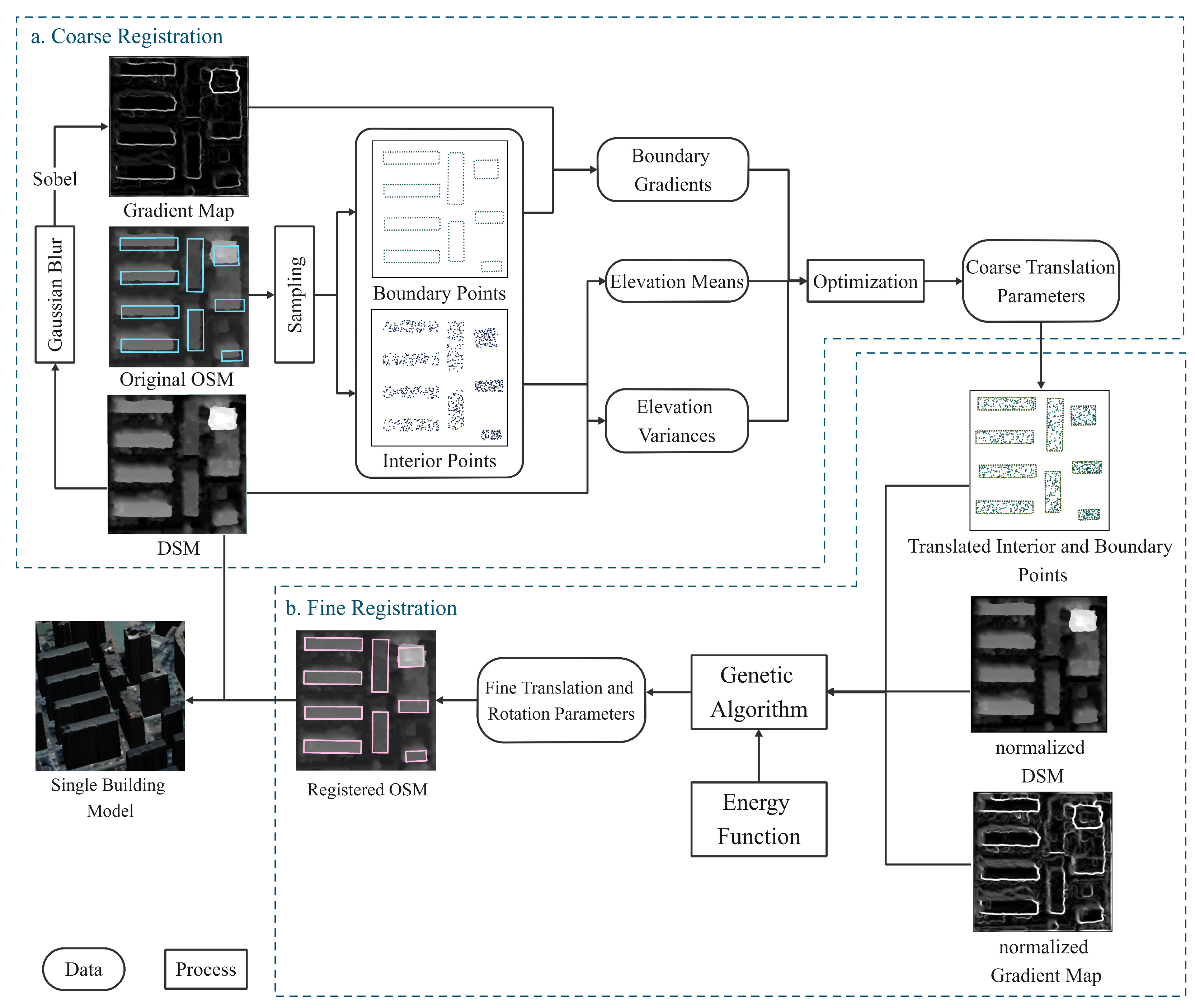
2.1. Workflow
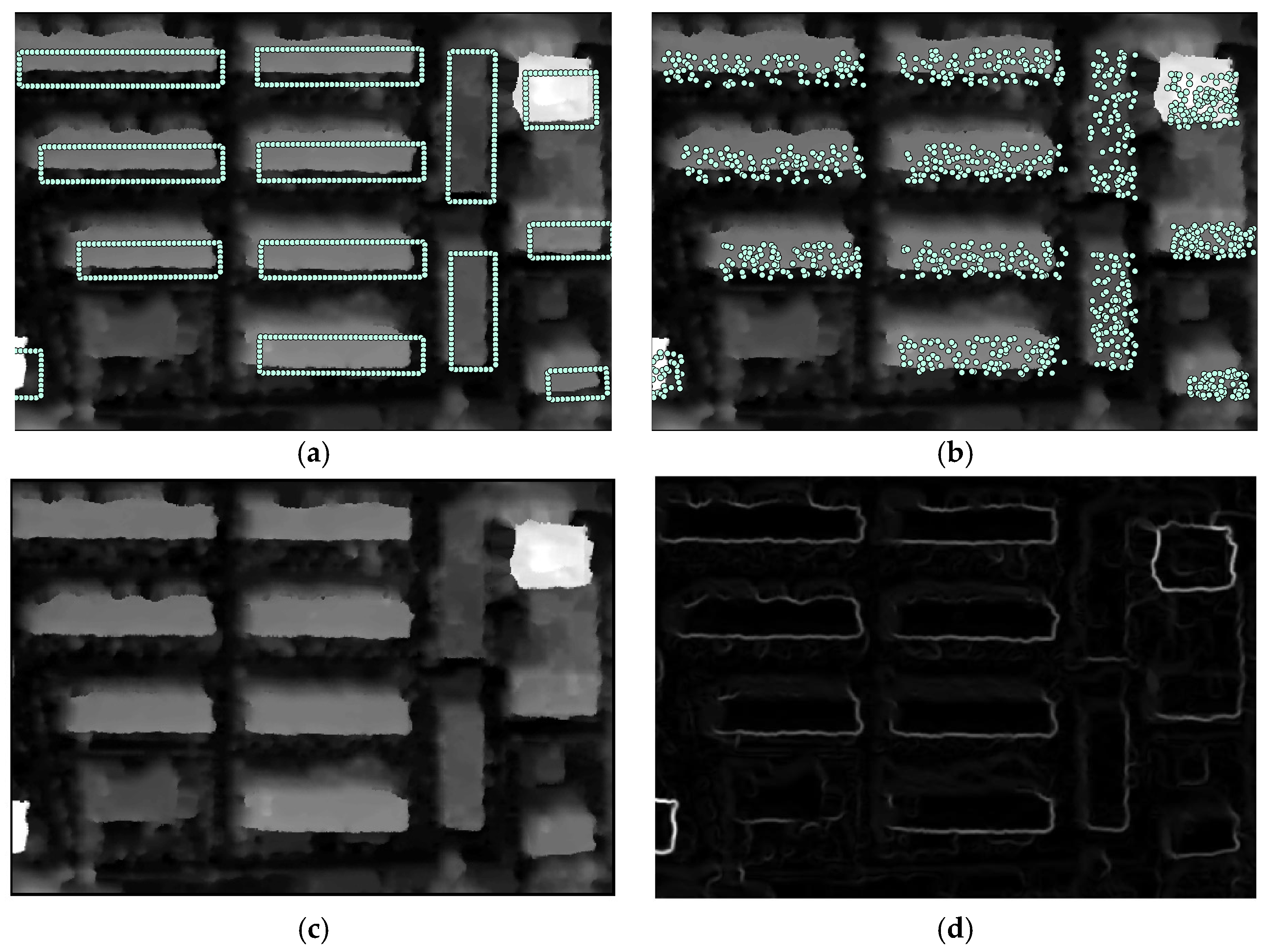
2.2. Coarse Registration
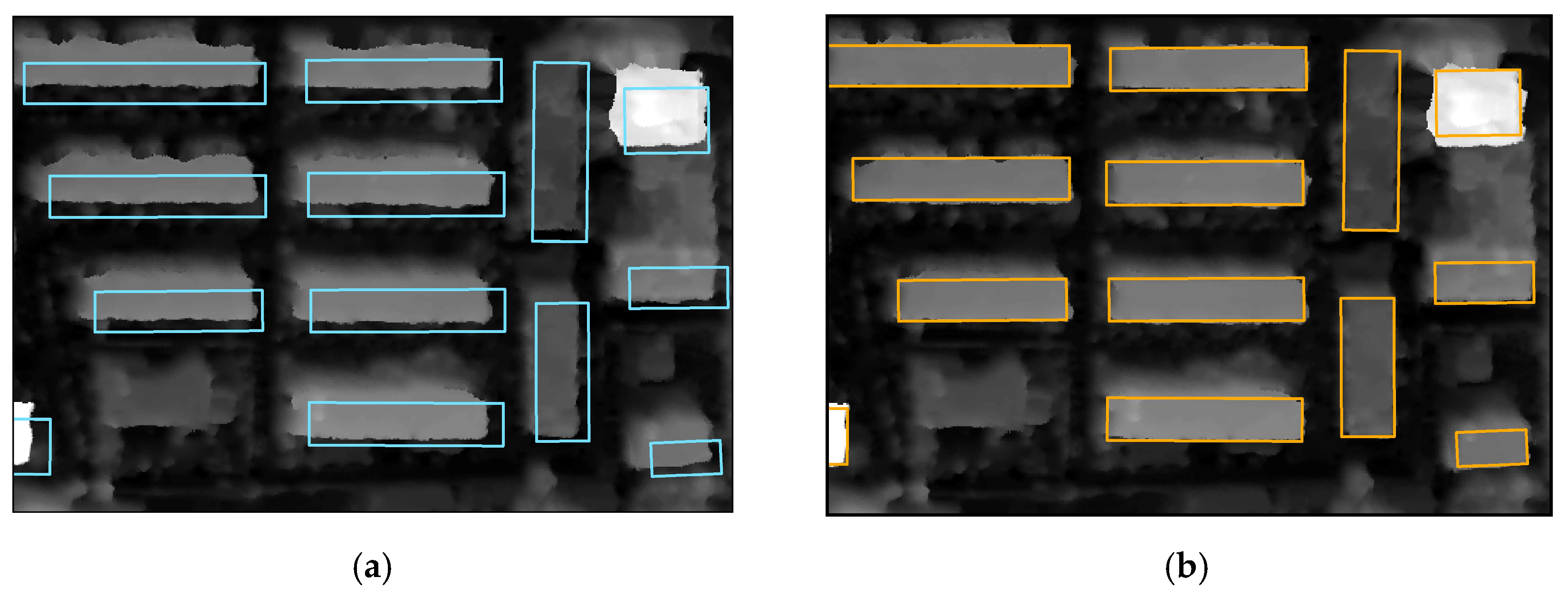
2.3. Fine Registration
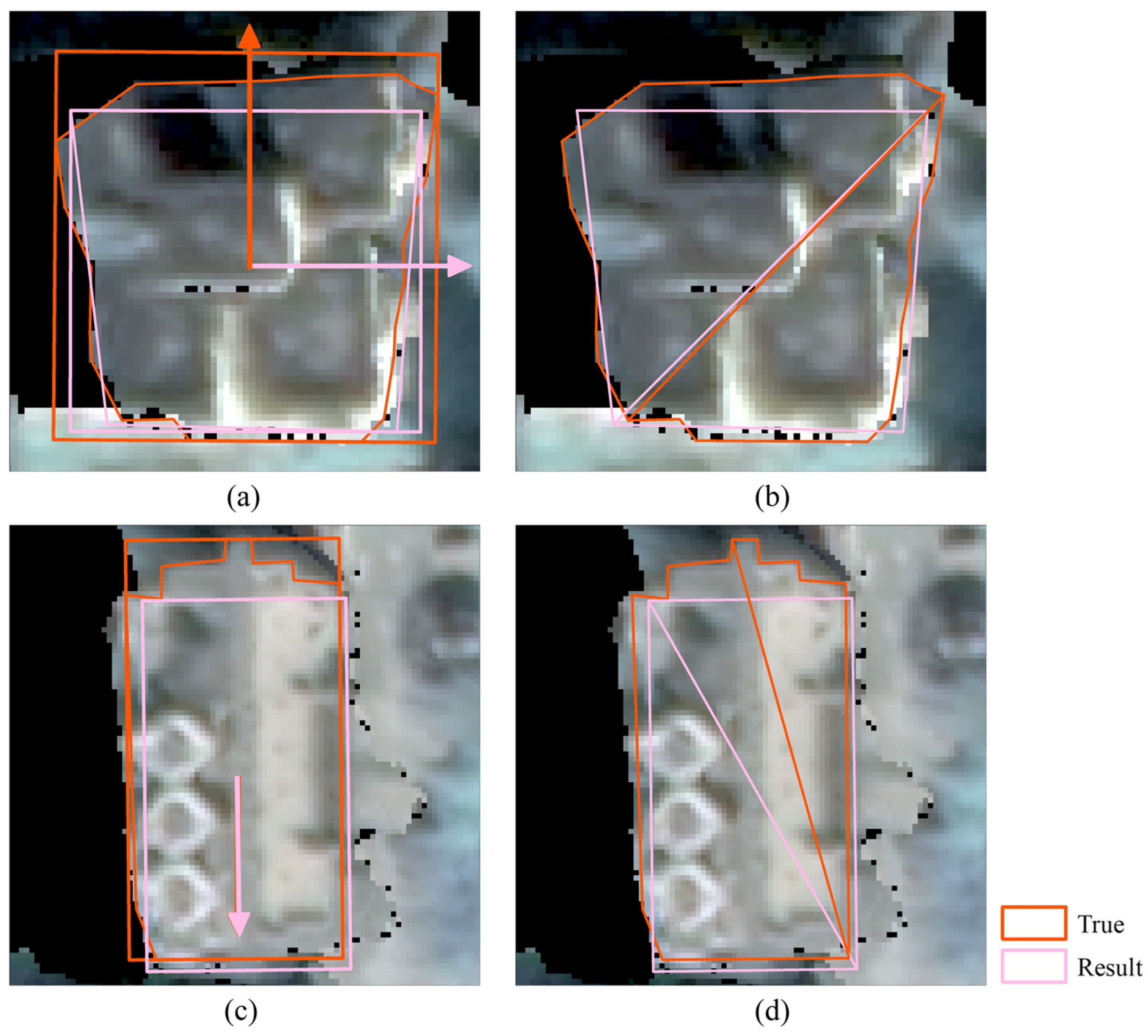
2.3.1. Formulation
2.3.2. Solution
2.4. Single Building Model Reconstruction
3. Experiments
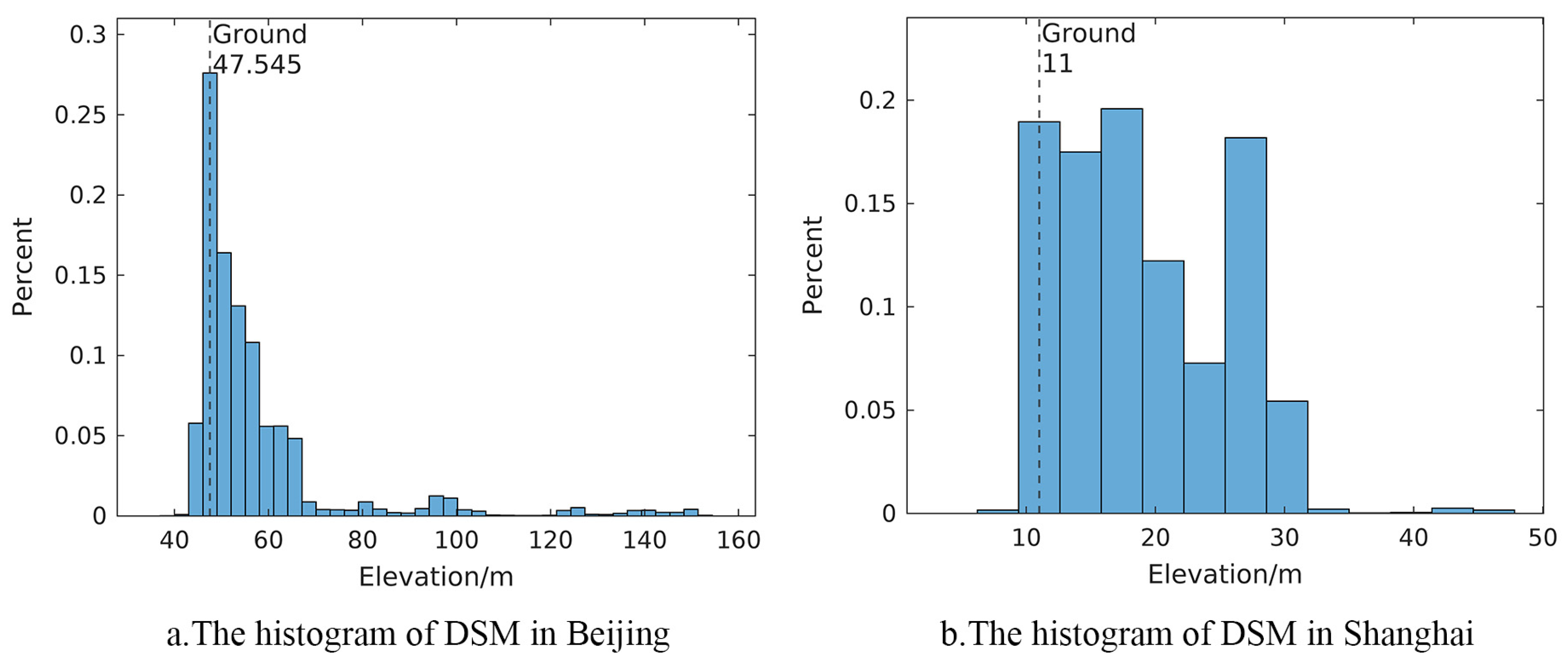
3.1. Study Regions and Datasets
3.2. Accuracy Evaluation Metrics
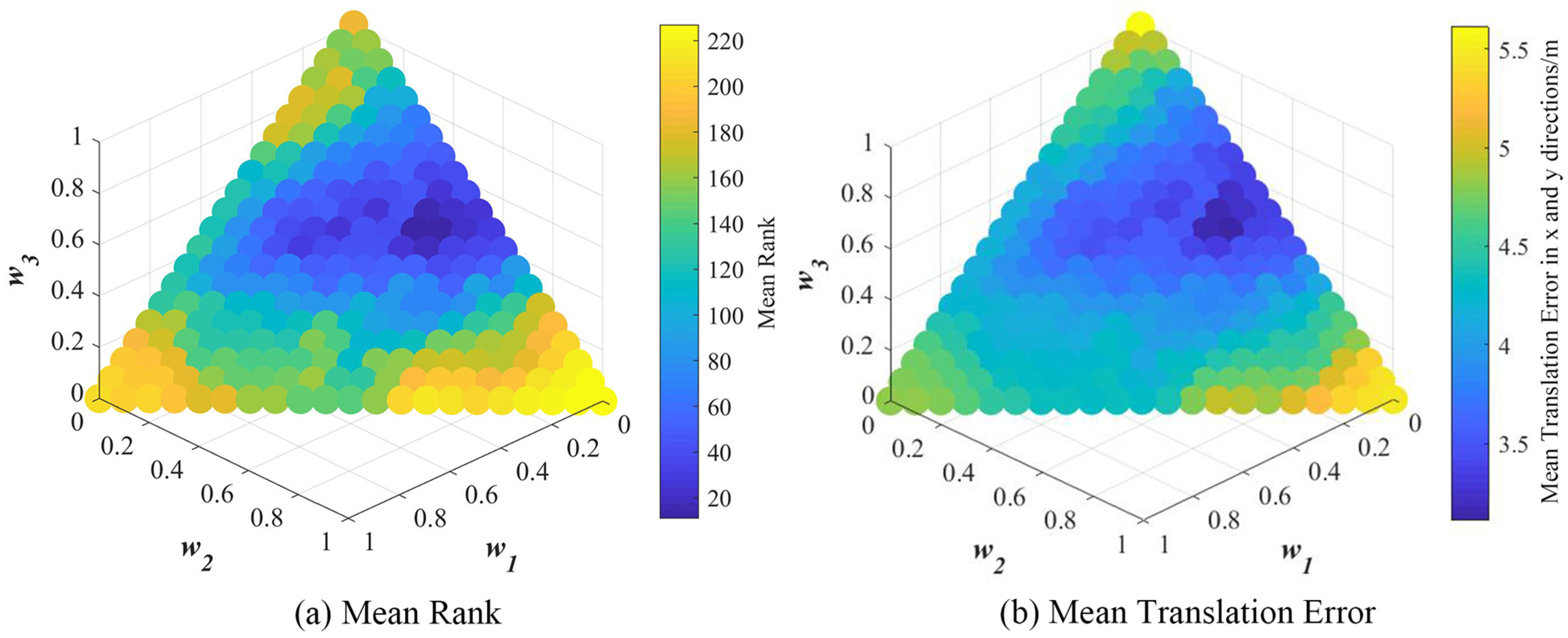
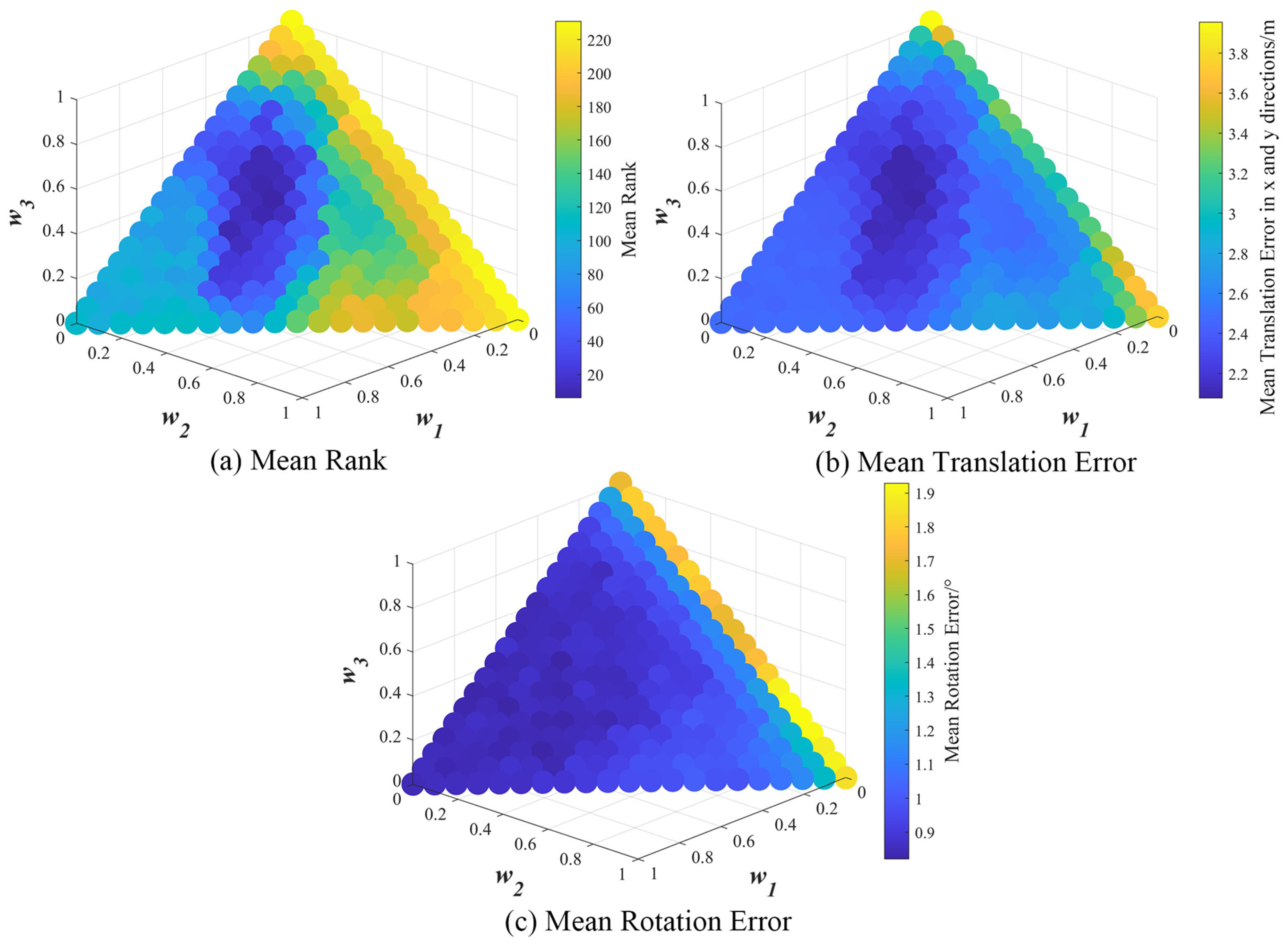
3.3. Parameters Optimization
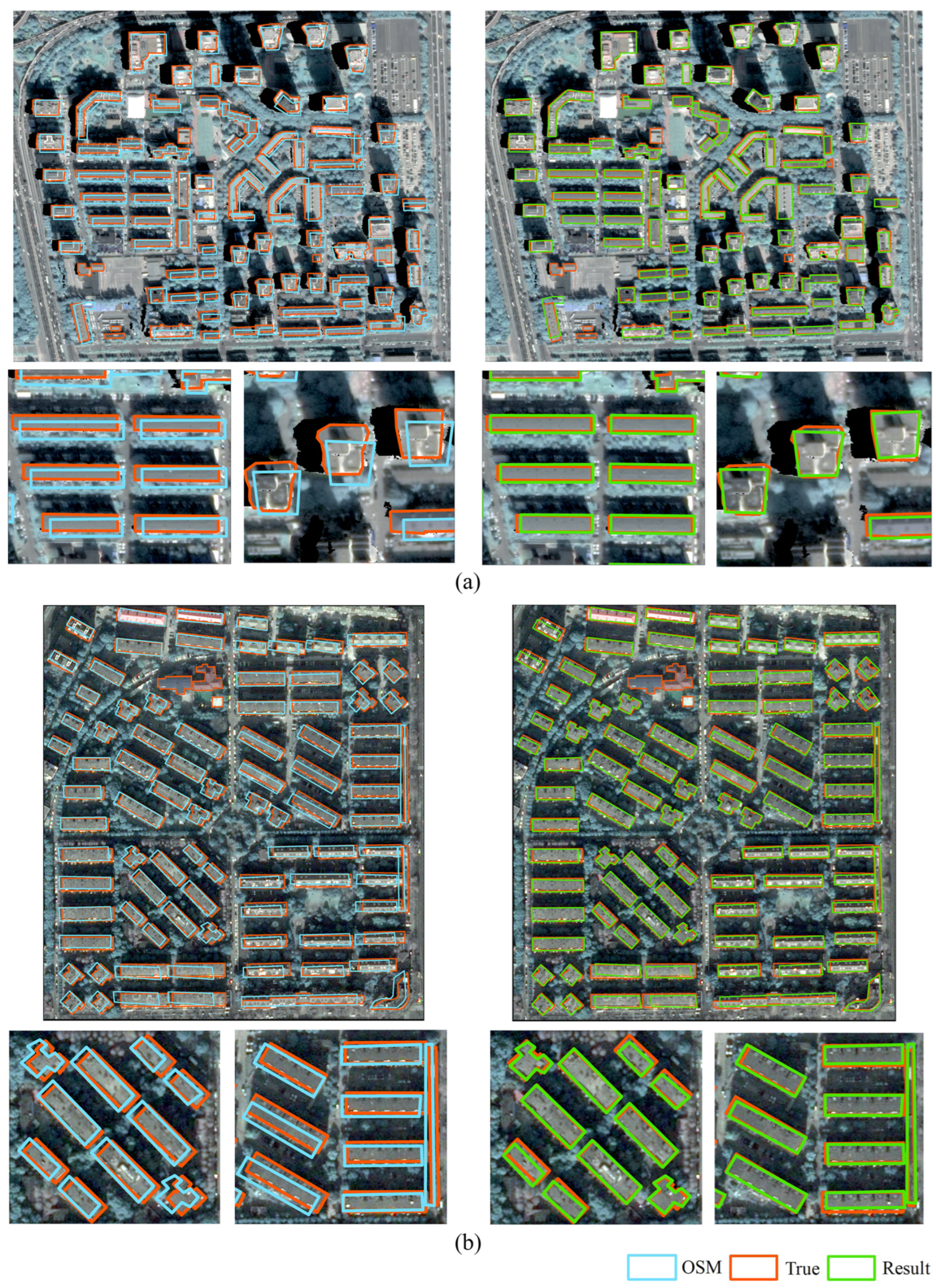
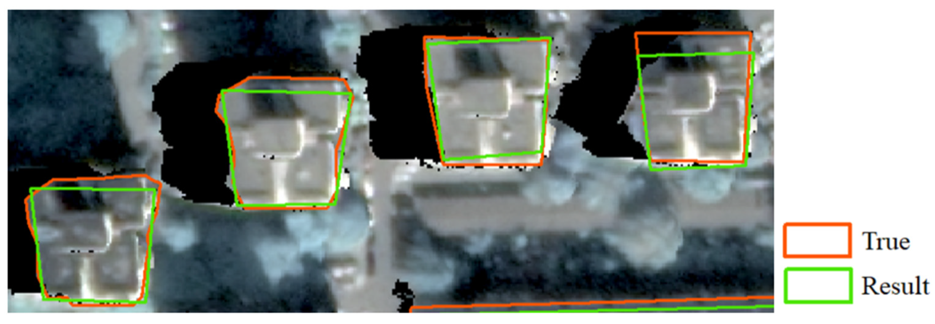
3.4. Experimental Result Analysis
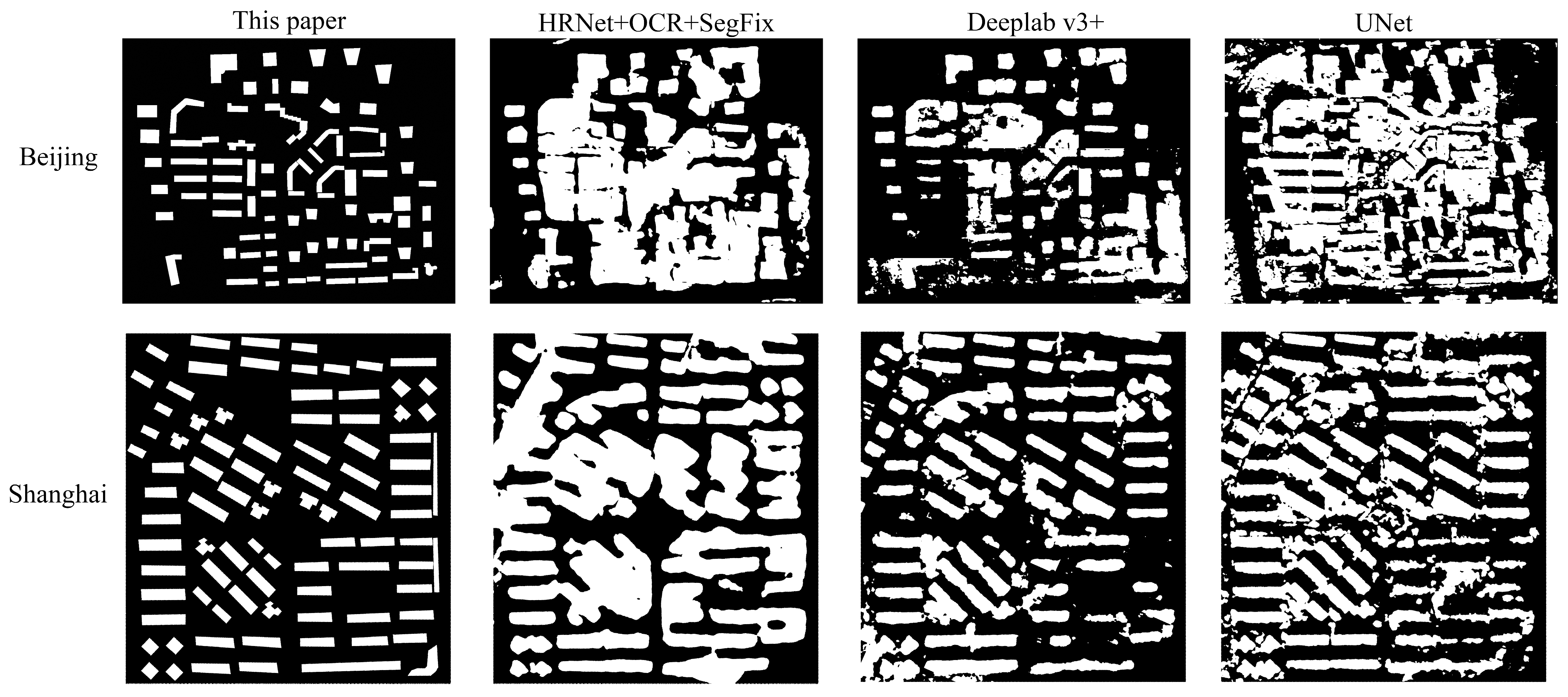
3.5. Comparison
4. Discussion
5. Conclusions
Author Contributions
Funding
Data Availability Statement
Acknowledgments
Conflicts of Interest
References
- Arroyo Ohori, K.; Biljecki, F.; Kumar, K.; Ledoux, H.; Stoter, J. Modeling cities and landscapes in 3D with CityGML. In Building Information Modeling; Springer: Berlin/Heidelberg, Germany, 2018; pp. 199–215. [Google Scholar]
- Gröger, G.; Kolbe, T.H.; Nagel, C.; Häfele, K.-H. OGC city geography markup language (CityGML) encoding standard. 2012. [Google Scholar]
- Duan, L.; Lafarge, F. Towards large-scale city reconstruction from satellites. In Proceedings of the European Conference on Computer Vision, Amsterdam, The Netherlands, 11–14 October 2016; pp. 89–104. [Google Scholar]
- Li, W.; Meng, L.; Wang, J.; He, C.; Xia, G.-S.; Lin, D. 3D Building Reconstruction from Monocular Remote Sensing Images. In Proceedings of the IEEE/CVF International Conference on Computer Vision, Montreal, BC, Canada, 11–17 October 2021; pp. 12548–12557. [Google Scholar]
- Pepe, M.; Costantino, D.; Alfio, V.S.; Vozza, G.; Cartellino, E. A Novel Method Based on Deep Learning, GIS and Geomatics Software for Building a 3D City Model from VHR Satellite Stereo Imagery. ISPRS Int. J. Geo-Inf. 2021, 10, 697. [Google Scholar] [CrossRef]
- Rajpriya, N.R.; Vyas, A.; Sharma, S.A. Generation of 3D Model for Urban area using Ikonos and Cartosat-1 Satellite Imageries with RS and GIS Techniques. ISPRS Int. Arch. Photogramm. Remote Sens. Spat. Inf. Sci. 2014, 40, 899–906. [Google Scholar] [CrossRef] [Green Version]
- Adreani, L.; Colombo, C.; Fanfani, M.; Nesi, P.; Pantaleo, G.; Pisanu, R. A Photorealistic 3D City Modeling Framework for Smart City Digital Twin. In Proceedings of the 2022 IEEE International Conference on Smart Computing (SMARTCOMP), Helsinki, Finland, 20–24 June 2022; pp. 299–304. [Google Scholar]
- Camacho, P.H.T.; Santiago, V.M.R.; Sarmiento, C.J.S. Semi-automatic generation of an lod1 and lod2 3d city model of Tanauan city, batangas using openstreetmap and taal open lidar data in qgis. ISPRS Int. Arch. Photogramm. Remote Sens. Spat. Inf. Sci. 2021, XLVI-4/W6-2021, 77–84. [Google Scholar] [CrossRef]
- Buyukdemircioglu, M.; Kocaman, S. A 3D campus application based on city models and webgl. ISPRS Int. Arch. Photogramm. Remote Sens. Spat. Inf. Sci. 2018, 42, 161–165. [Google Scholar] [CrossRef] [Green Version]
- Pepe, M.; Costantino, D.; Alfio, V.S.; Angelini, M.G.; Garofalo, A.R. A CityGML Multiscale Approach for the Conservation and Management of Cultural Heritage: The Case Study of the Old Town of Taranto (Italy). ISPRS Int. J. Geo-Inf. 2020, 9, 449. [Google Scholar] [CrossRef]
- Aditya, T.; Laksono, D. LOD 1: 3D CityModel for Implementing SmartCity Concept. In Proceedings of the 2017 International Conference on Information Technology, Singapore, 27–29 December 2017; pp. 136–141. [Google Scholar]
- Luo, H.; He, B.; Guo, R.; Wang, W.; Kuai, X.; Xia, B.; Wan, Y.; Ma, D.; Xie, L. Urban Building Extraction and Modeling Using GF-7 DLC and MUX Images. Remote Sens. 2021, 13, 3414. [Google Scholar] [CrossRef]
- Sharma, S.A.; Agrawal, R.; Jayaprasad, P. Development of ‘3D city models’ using IRS satellite data. J. Indian Soc. Remote Sens. 2016, 44, 187–196. [Google Scholar] [CrossRef]
- Danchao, G.; Yilong, H.; Xu, H. Global refinement of building boundary with line feature constraints for stereo dense image matching. Acta Geod. Et Cartogr. Sin. 2021, 50, 833. [Google Scholar]
- Tripodi, S.; Duan, L.; Trastour, F.; Poujad, V.; Laurore, L.; Tarabalka, Y. Automated chain for large-scale 3d reconstruction of urban scenes from satellite images. ISPRS Int. Arch. Photogramm. Remote Sens. Spat. Inf. Sci. 2019, 42, 243–250. [Google Scholar] [CrossRef] [Green Version]
- Rastogi, K.; Bodani, P.; Sharma, S.A. Automatic building footprint extraction from very high-resolution imagery using deep learning techniques. Geocarto Int. 2020, 37, 1501–1513. [Google Scholar] [CrossRef]
- Xu, Y.; Wu, L.; Xie, Z.; Chen, Z. Building Extraction in Very High Resolution Remote Sensing Imagery Using Deep Learning and Guided Filters. Remote Sens. 2018, 10, 144. [Google Scholar] [CrossRef] [Green Version]
- Tripodi, S.; Duan, L.; Poujade, V.; Trastour, F.; Bauchet, J.-P.; Laurore, L.; Tarabalka, Y. Operational pipeline for large-scale 3D reconstruction of buildings from satellite images. In Proceedings of the IGARSS 2020–2020 IEEE International Geoscience and Remote Sensing Symposium, Waikoloa, HI, USA, 26 September–2 October 2020; pp. 445–448. [Google Scholar]
- Sadeq, H.; Drummond, J.; Li, Z. Utilizing Satellite Optical Imagery for Building Footprint Extraction and City Modelling; University of Glasgow: Glasgow, UK, 2014. [Google Scholar]
- Yu, D.; Ji, S.; Liu, J.; Wei, S. Automatic 3D building reconstruction from multi-view aerial images with deep learning. ISPRS J. Photogramm. Remote Sens. 2020, 171, 155–170. [Google Scholar] [CrossRef]
- Yu, D.; Wei, S.; Liu, J.; Ji, S. Advanced approach for automatic reconstruction of 3d buildings from aerial images. ISPRS Int. Arch. Photogramm. Remote Sens. Spat. Inf. Sci. 2020, 43, 541–546. [Google Scholar] [CrossRef]
- Partovi, T.; Fraundorfer, F.; Bahmanyar, R.; Huang, H.; Reinartz, P. Automatic 3-D Building Model Reconstruction from Very High Resolution Stereo Satellite Imagery. Remote Sens. 2019, 11, 1660. [Google Scholar] [CrossRef] [Green Version]
- Wang, Y.; Zorzi, S.; Bittner, K. Machine-learned 3D building vectorization from satellite imagery. In Proceedings of the Proceedings of the IEEE/CVF Conference on Computer Vision and Pattern Recognition, Nashville, TN, USA, 20–25 June 2021; pp. 1072–1081. [Google Scholar]
- Woo, D.-M.; Park, D.-C. Stereoscopic Building Reconstruction Using High-Resolution Satellite Image Data. In Proceedings of the 2011 10th IEEE/ACIS International Conference on Computer and Information Science, Sanya, China, 16–18 May 2011; pp. 194–198. [Google Scholar]
- Pan, Z.; Xu, J.; Guo, Y.; Hu, Y.; Wang, G. Deep Learning Segmentation and Classification for Urban Village Using a Worldview Satellite Image Based on U-Net. Remote Sens. 2020, 12, 1574. [Google Scholar] [CrossRef]
- Li, W.; He, C.; Fang, J.; Zheng, J.; Fu, H.; Yu, L. Semantic Segmentation-Based Building Footprint Extraction Using Very High-Resolution Satellite Images and Multi-Source GIS Data. Remote Sens. 2019, 11, 403. [Google Scholar] [CrossRef] [Green Version]
- Gui, S.; Qin, R. Automated LoD-2 model reconstruction from very-high-resolution satellite-derived digital surface model and orthophoto. ISPRS J. Photogramm. Remote Sens. 2021, 181, 1–19. [Google Scholar] [CrossRef]
- Esch, T.; Zeidler, J.; Palacios-Lopez, D.; Marconcini, M.; Roth, A.; Mönks, M.; Leutner, B.; Brzoska, E.; Metz-Marconcini, A.; Bachofer, F.; et al. Towards a Large-Scale 3D Modeling of the Built Environment—Joint Analysis of TanDEM-X, Sentinel-2 and Open Street Map Data. Remote Sens. 2020, 12, 2391. [Google Scholar] [CrossRef]
- Cavalagli, N.; Kita, A.; Falco, S.; Trillo, F.; Costantini, M.; Ubertini, F. Satellite radar interferometry and in-situ measurements for static monitoring of historical monuments: The case of Gubbio, Italy. Remote Sens. Environ. 2019, 235, 111453. [Google Scholar] [CrossRef]
- Bagheri, H.; Schmitt, M.; Zhu, X. Fusion of Multi-Sensor-Derived Heights and OSM-Derived Building Footprints for Urban 3D Reconstruction. ISPRS Int. J. Geo-Inf. 2019, 8, 193. [Google Scholar] [CrossRef] [Green Version]
- Goetz, M. Towards generating highly detailed 3D CityGML models from OpenStreetMap. Int. J. Geogr. Inf. Sci. 2013, 27, 845–865. [Google Scholar] [CrossRef]
- Kabolizade, M.; Ebadi, H.; Mohammadzadeh, A. Design and implementation of an algorithm for automatic 3D reconstruction of building models using genetic algorithm. Int. J. Appl. Earth Obs. Geoinf. 2012, 19, 104–114. [Google Scholar] [CrossRef]
- Mirjalili, S. Genetic algorithm. In Evolutionary Algorithms and Neural Networks; Springer: Berlin/Heidelberg, Germany, 2019; pp. 43–55. [Google Scholar]
- Whitley, D. A genetic algorithm tutorial. Stat. Comput. 1994, 4, 65–85. [Google Scholar] [CrossRef]
- Lambora, A.; Gupta, K.; Chopra, K. Genetic algorithm-A literature review. In Proceedings of the 2019 International Conference on Machine Learning, Big Data, Cloud and Parallel Computing (COMITCon), Faridabad, India, 14–16 February 2019; pp. 380–384. [Google Scholar]
- Holland, J. Genetic algorithms. Sci. Am. 1992, 267, 66–73. [Google Scholar] [CrossRef]
- Kanopoulos, N.; Vasanthavada, N.; Baker, R. Design of an image edge detection filter using the Sobel operator. IEEE J. Solid-State Circuits 1988, 23, 358–367. [Google Scholar] [CrossRef]
- Vincent, O.R.; Folorunso, O. A descriptive algorithm for sobel image edge detection. In Proceedings of the Informing Science & IT Education Conference (InSITE), Madrid, Spain, 16–18 November 2009; pp. 97–107. [Google Scholar]
- Vairalkar, M.K.; Nimbhorkar, S. Edge detection of images using Sobel operator. Int. J. Emerg. Technol. Adv. Eng. 2012, 2, 291–293. [Google Scholar]
- Lehmann, I.; Mathey, J.; Rößler, S.; Bräuer, A.; Goldberg, V. Urban vegetation structure types as a methodological approach for identifying ecosystem services—Application to the analysis of micro-climatic effects. Ecol. Indic. 2014, 42, 58–72. [Google Scholar] [CrossRef]
- Abdullah, S.R.; Omar, B.; Mohd Salleh, A.F.; Marwi, M.A.; Othman, H.; Wahid, S. Fly Colonization and Carcass Decomposition in a High-Rise Building in Malaysia. Int. Med. J. 2016, 23, 94–99. [Google Scholar]
- Huang, X.; Han, Y.; Hu, K. An improved semi-global matching method with optimized matching aggregation constraint. In Proceedings of the 2020 The Third International Workshop on Environment and Geoscience, Chengdu, China, 18–20 July 2020; p. 569. [Google Scholar] [CrossRef]
- Gong, D.; Huang, X.; Zhang, J.; Yao, Y.; Han, Y. Efficient and Robust Feature Matching for High-Resolution Satellite Stereos. Remote Sens. 2022, 14, 5617. [Google Scholar] [CrossRef]
- Bosch, M.; Foster, K.; Christie, G.; Wang, S.; Hager, G.D.; Brown, M. Semantic stereo for incidental satellite images. In Proceedings of the 2019 IEEE Winter Conference on Applications of Computer Vision (WACV), Waikoloa Village, HI, USA, 7–11 January 2019; pp. 1524–1532. [Google Scholar]
- Le Saux, B.; Yokoya, N.; Hansch, R.; Brown, M.; Hager, G. 2019 Data Fusion Contest [Technical Committees]. IEEE Geosci. Remote Sens. Mag. 2019, 7, 103–105. [Google Scholar] [CrossRef]
- Syarif, I.; Prugel-Bennett, A.; Wills, G. SVM Parameter Optimization using Grid Search and Genetic Algorithm to Improve Classification Performance. Telkomnika Telecommun. Comput. Electron. Control. 2016, 14, 1502. [Google Scholar] [CrossRef]
- Yuan, Y.; Chen, X.; Chen, X.; Wang, J. Segmentation transformer: Object-contextual representations for semantic segmentation. arXiv 2019, arXiv:1909.11065. [Google Scholar]
- Chen, L.-C.; Zhu, Y.; Papandreou, G.; Schroff, F.; Adam, H. Encoder-decoder with atrous separable convolution for semantic image segmentation. In Proceedings of the European Conference on Computer Vision (ECCV), Munich, Germany, 8–14 September 2018; pp. 801–818. [Google Scholar]
- Ronneberger, O.; Fischer, P.; Brox, T. U-net: Convolutional networks for biomedical image segmentation. In Proceedings of the International Conference on Medical Image Computing and Computer-Assisted Intervention, Munich, Germany, 5–9 October 2015; pp. 234–241. [Google Scholar]
- Bozzano, F.; Esposito, C.; Mazzanti, P.; Patti, M.; Scancella, S. Imaging Multi-Age Construction Settlement Behaviour by Advanced SAR Interferometry. Remote Sens. 2018, 10, 1137. [Google Scholar] [CrossRef] [Green Version]
- Crosetto, M.; Monserrat, O.; Cuevas-González, M.; Devanthéry, N.; Crippa, B. Persistent Scatterer Interferometry: A review. ISPRS J. Photogramm. Remote Sens. 2016, 115, 78–89. [Google Scholar] [CrossRef] [Green Version]


| Jacksonville | Beijing | Shanghai | |
|---|---|---|---|
| Area (km2) | 0.87 | 0.45 | 0.21 |
| Number of buildings | 187 | 84 | 88 |
| Region | IoU | Precision | Recall | F1-Score | ΔC/m | Δθ/° | ||
|---|---|---|---|---|---|---|---|---|
| Beijing | Before | 0.454 | 0.627 | 0.605 | 0.613 | 0.012 | 6.900 | 1.654 |
| After | 0.771 | 0.884 | 0.853 | 0.875 | 0.655 | 2.244 | 1.116 | |
| Shanghai | Before | 0.618 | 0.794 | 0.724 | 0.754 | 0.148 | 4.388 | 1.340 |
| After | 0.780 | 0.917 | 0.840 | 0.873 | 0.659 | 1.573 | 1.112 |
| Region | Metric | Ours | HRNet + OCR + SegFix | Deeplab v3+ | UNet |
|---|---|---|---|---|---|
| Beijing | IoU | 0.775 | 0.331 | 0.457 | 0.290 |
| Precision | 0.895 | 0.335 | 0.495 | 0.295 | |
| Recall | 0.852 | 0.964 | 0.857 | 0.948 | |
| F1-score | 0.873 | 0.498 | 0.628 | 0.450 | |
| Shanghai | IoU | 0.774 | 0.462 | 0.599 | 0.518 |
| Precision | 0.924 | 0.476 | 0.672 | 0.561 | |
| Recall | 0.827 | 0.943 | 0.847 | 0.870 | |
| F1-score | 0.873 | 0.633 | 0.749 | 0.682 |
Disclaimer/Publisher’s Note: The statements, opinions and data contained in all publications are solely those of the individual author(s) and contributor(s) and not of MDPI and/or the editor(s). MDPI and/or the editor(s) disclaim responsibility for any injury to people or property resulting from any ideas, methods, instructions or products referred to in the content. |
© 2023 by the authors. Licensee MDPI, Basel, Switzerland. This article is an open access article distributed under the terms and conditions of the Creative Commons Attribution (CC BY) license (https://creativecommons.org/licenses/by/4.0/).
Share and Cite
He, Y.; Liao, W.; Hong, H.; Huang, X. High-Precision Single Building Model Reconstruction Based on the Registration between OSM and DSM from Satellite Stereos. Remote Sens. 2023, 15, 1443. https://doi.org/10.3390/rs15051443
He Y, Liao W, Hong H, Huang X. High-Precision Single Building Model Reconstruction Based on the Registration between OSM and DSM from Satellite Stereos. Remote Sensing. 2023; 15(5):1443. https://doi.org/10.3390/rs15051443
Chicago/Turabian StyleHe, Yong, Wenting Liao, Hao Hong, and Xu Huang. 2023. "High-Precision Single Building Model Reconstruction Based on the Registration between OSM and DSM from Satellite Stereos" Remote Sensing 15, no. 5: 1443. https://doi.org/10.3390/rs15051443