Accurate and Serialized Dense Point Cloud Reconstruction for Aerial Video Sequences

Abstract

Traditional multi-view stereo (MVS) is not applicable for the point cloud reconstruction of serialized video frames. Among them, the exhausted feature extraction and matching for all the prepared frames are time-consuming, and the scope of the search requires covering all the key frames. In this paper, we propose a novel serialized reconstruction method to solve the above issues. Specifically, a joint feature descriptors-based covisibility cluster generation strategy is designed to accelerate the feature matching and improve the performance of the pose estimation. Then, a serialized structure-from-motion (SfM) and dense point cloud reconstruction framework is designed to achieve high efficiency and competitive precision reconstruction for serialized frames. To fully demonstrate the superiority of our method, we collect a public aerial sequences dataset with referable ground truth for the dense point cloud reconstruction evaluation. Through a time complexity analysis and the experimental validation in this dataset, the comprehensive performance of our algorithm is better than the other compared outstanding methods.

1. Introduction

Dense point cloud reconstruction for aerial video sequences has been a long-standing problem in computer vision and remote sensing. It is worth noting that there is no difference between the 3D reconstruction of an aerial image and multi-view in processing. However, in terms of input data, the baselines between aerial images are wider and larger, and it is easy to have a dynamic blur that needs to be preprocessed. There are many high-quality methods that can accurately generate a semi-dense (or dense) point cloud. However, it is still a great challenge to balance the reconstruction accuracy and efficiency, especially for a large-scale complex aerial scene reconstruction in practical applications.

Studies over the past two decades have proposed a considerable amount of methods trying to solve the above issue. The commercial 3D reconstruction systems, such as Google Earth, Apple Map and OpenStreetMap, can provide high-quality reconstruction but cost too much. Agisoft PhotoScan, as the best commercial point cloud reconstruction software, can achieve dense modeling based on disordered images. However, its slow speed seriously limits the development of the practical application.

Starting with the feature matching of image pairs, most of the multi-view point cloud reconstruction strategies utilize the structure from motion (SfM) for camera parameters estimation and sparse reconstruction. Then, a semi-dense or dense point cloud is expanded by applying multi-view stereo (MVS). Among them, some good progress has been made by combining the advantages of various types of a high-performance SfM and accelerated the reconstruction process of the traditional SfM by using a shared rotation averaging method with a bundle adjustment, such as the work of [1] who proposed a new pose estimation method for Rolling Shutter cameras. The deformation of the rigid 3D template in the RS camera can be viewed as a non-rigid deformable 3D template captured by the GS camera. So as to achieve high-quality attitude and instantaneous self-motion parameters of the RS camera, Ravendran et al. [2] proposed a direct method for image registration within bursts of short exposure time images to improve the robustness and accuracy of motion feature-based structures (SfM). They solved the problem of image processing under low light conditions and improved the performance of the SfM in light-limited scenes. However, SfM is over-reliant on feature matching, which requires exhaustive image pair matching for all prepared image frames to ensure the accuracy of the reconstruction, which will bring redundant operations. For a dense point cloud reconstruction, a patch-based multi-view stereo method (PMVS) [3] is usually applied, which repeatedly expands a sparse set of matched key points until visibility constraints are invoked to filter away false matches. Based on PMVS, Wu [4] proposed a matching method (Visual-SfM) with accelerated SfM and PMVS to realize fast semi-dense reconstruction. Furthermore, COLMAP [5] provided a revised structure-from-motion (SfM) and multi-view stereo (MVS) pipeline for high-quality dense point cloud reconstruction; this method is now considered as the state-of-the-art MVS method. However, these methods aim at reconstructing a global 3D model by using all the images (in this paper, images are instead key frames) available simultaneously; thus, they suffer from the scalability problem as the number of images grows.

In addition, a simultaneous localization and mapping (SLAM) system is one of the hot research topics in the robotics and computer vision community, which can achieve real-time sparse point cloud reconstruction for serialized video frames. Nevertheless, the original intention of SLAM is not for reconstruction but to use very sparse 3D point clouds to locate and navigate the robot in limited space. Recently, people began to focus on researching SLAM-based dense point cloud reconstruction applications. There are many excellent methods being proposed, such as DRM-SLAM [6] and ROS-based Monocular SLAM [7]. Unfortunately, most of them are not pure visual-based methods, which require third-party depth information or sensors to achieve a dense reconstruction for an indoor scene or single target [8,9]. Some pure visual SLAM systems are designed for large-scale scene 3D reconstruction and to achieve a good performance, such as Blitz SLAM [10] where a semantic SLAM system suitable for indoor dynamic environments was presented. Combining the advantages of a mask and the semantic and geometric information of RGB images, the large scenic spot cloud reconstruction with dynamic targets can be realized. Recently, implicit characterization has shown exciting results in various fields, including promising advances in SLAM [11,12,13]. However, the existing methods based on a neural radiation field produce an overly smooth scene reconstruction and are difficult to extend to large scenes. It can be seen that without using sensors or external depth information, an RGB images-based pure visual SLAM cannot provide a high-accuracy dense reconstruction in large-scale outdoor scenes. Therefore, this paper does not give a comparative experiment with pure visual-based SLAM methods. The deep learning-based methods have proved the potential capacity of 3D point cloud reconstruction through end-to-end depth estimation. In the real world, depth data acquired by, for example, RGB-D cameras, stereo vision and laser scanners are generally sparse and vary in the degree of sparsity. To complement the depth values with different degrees of sparsity, Uhrig et al. [14] proposed a sparse invariant convolutional neural network (CNN) and applied it to the depth upsampling of sparse laser scan data. It explicitly considers the location of missing data in the convolution operation and introduces a novel sparse convolution layer (sparse convolution, SparConv). It weights the elements of the convolution kernel according to the validity of the input pixels and passes the pixel validity information to the subsequent layers of the network. This allows the method to handle varying degrees of sparse data without a significant loss of accuracy. Similarly, Huang et al. [15] proposed three new sparse-invariant operations in order to effectively utilize multiscale features in neural networks and designed a sparse-invariant multiscale decoder network (Hierarchical multi-scale, HMS-Net) to handle sparse inputs based on this.

For the prediction from sparse to dense depths, the depth values of sparse samples should be preserved because they usually come from reliable sensors; also, the transition between sparse depth samples and their neighboring depths should be smooth and natural. Considering the above two points, Cheng et al. [16] proposed a simple and effective Convolutional Spatial Propagation Network (CSPN) to learn the similarity matrix for depth prediction. Specifically, an effective linear propagation model was used in the paper, which is propagated by recursive convolutional operations and learns the similarity between neighboring pixels by using a deep convolutional neural network (CNN) to achieve a more accurate depth estimation and it can run in real time. However, multiple spatial pooling operations lead to an increasingly low resolution of the feature maps; multi-layer deconvolution operations complicate the network training and consume more computation. To solve the above problems, Fu et al. [17] proposed the Deep Ordinal Regression Network (DORN) and introduced the spacing-increasing discretization (SID) strategy. Specifically, the uncertainty of the depth prediction increases with the depth of the true value, i.e., a relatively large error should be allowed in predicting larger depth values to avoid the excessive impact of too-large depth values on the training process. Therefore, the continuous depth is discretized into multiple intervals in the paper, and the deep network learning is converted into a sequential regression problem.

In terms of the input to the network, inputting only RGB images for the depth estimation of a single image is itself an ill-posed problem with large limitations. In view of this, Chen et al. [18] proposed the Deep Depth Densification (D3) module, which considers both sparse depth and RGB images as inputs for a dense depth estimation. Similar to the idea proposed by Fu et al. [17], considering that points farther away from a known-depth pixel tend to produce higher residuals, Chen et al. parametrized the sparse depth input so that it can adapt to arbitrary sparse depth patterns. Similarly, Shivakumar et al. [19] attempted to gather contextual information from high-resolution RGB images by upsampling a series of sparse range measurements. They proposed Deep Fusion Net (DFuseNet) which uses a two-branch architecture for the fusion of RGB images and sparse depths as a way to obtain dense depth estimates. The learning of contextual information is performed with the help of a Spatial Pyramid Pooling (SPP) module. Similarly, Mal et al. [20] considered images from a sparse set of depth measurements and a single RGB for dense depth prediction. They proposed using a single-depth regression network to learn the data directly from the RGB-D raw and explore the effect of the number of sample depths on the prediction accuracy. The article uses a deep residual network (ResNet) as the basic network structure but removes its last mean-merge and linear transformation layers, uses the mean absolute error as the loss function and performs depth sampling by the Bernoulli probability to demonstrate the effect of different depth samples on depth prediction. It is noted in the paper that the prediction accuracy of the method is substantially better than the existing methods, including RGB-based and fusion-based techniques. In addition, the method can be used as a plug-in module to load sparse visual odometry/SLAM algorithms to create accurate dense point clouds. However, these methods often require a large amount of data for training, which is very time-consuming and has a poor generalization performance. In contrast to dense point cloud reconstruction, deep convolutional neural networks (CNN) are better for feature extraction, which can be used to improve the performance of image matching.

In this paper, our goal is to develop accurate and fast dense point cloud reconstruction for aerial video sequences by taking both high accuracy and efficiency into account. As traditional SfM-based MVS methods suffer from the scalability problem (exhaustive image pair matching) and visual SLAM based on RGB images cannot be directly used for real-time dense reconstruction, we adopt novel serialized feature matching and dense point cloud reconstruction for aerial video sequences with a temporal and spatial correlation between frames, where deep feature descriptors are also introduced to generate the covisibility cluster and detect the loop closure.

In brief, the main contributions are summarized as follows:

• A joint feature descriptors-based covisibility cluster generation strategy: To accelerate the feature matching and improve the performance of the pose estimation, we propose a novel covisibility cluster generation strategy (inspired by real-time SLAM methods) as the nearest neighbor frames constraint, which incorporates traditional feature descriptors and deep feature descriptors to apply a temporal and spatial correlation search, respectively.
• A serialized structure-from-motion (SfM) and dense point cloud reconstruction framework with high efficiency and competitive precision: In contrast to the exhausted feature matching of the traditional Sfm, we proposed a novel serialized SfM based on the covisibility cluster of a new frame, which provides pose optimization for loop closure detection by using deep feature descriptors instead of bag of words. Furthermore, serialized patch match and depth fusion strategies are applied for accurate and fast dense point cloud reconstruction.
• A public aerial sequences dataset with referable ground truth for dense point cloud reconstruction evaluation: We collect a publicly available aerial sequences (with Scenes 1–3) dataset with referable camera poses and dense point clouds for evaluation. Through a time complexity analysis and the experimental validation in this dataset, we show that the comprehensive performance of our algorithm is better than the other compared outstanding methods.

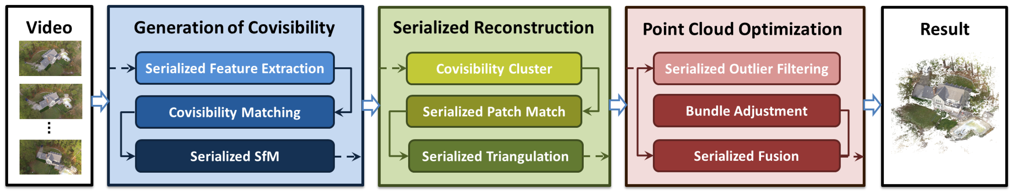
2. Proposed Method

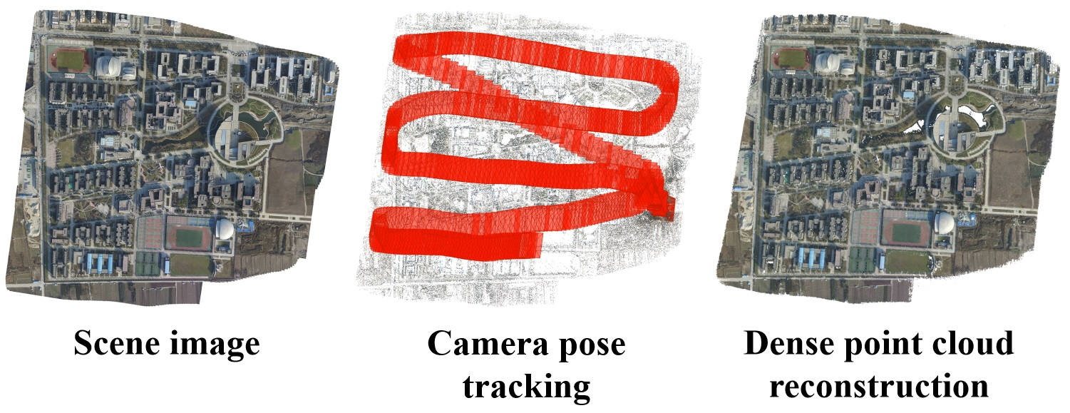
As shown in Figure 1, there are three main threads in our method running alternately until all the sub-point clouds have been fused to obtain a completed point cloud. The input data of this work are oblique aerial videos (serialized images: there is a time-series relationship between the key frames of aerial video) of UAV. The track of aerial shooting needs special planning in advance to obtain sufficient overlap to ensure the integrity and density of reconstruction. After video collection is completed, data preprocessing should be carried out, including key frames extraction, video frames selection and dynamic blur removal and so on. Firstly, the current key frame is assigned a covisibility cluster in the image sequence. Secondly, dense point clouds of the current frame are generated by serialized patch matching algorithm constrained by covisibility cluster. Finally, current sub-point clouds are added to a serialized consistency optimization queue to incrementally construct a complete dense 3D point cloud. Later, we will introduce the specific techniques in each step as below:

2.1. Generation of the Covisibility Cluster

Given a new sequential frame, a covisibility cluster corresponding to the current frame will be collected from the input frames ahead of the current one by considering the consistency of time and space fields. The covisibility cluster acts as a search range to constrain our serialized feature matching, depth estimation and point cloud reconstruction.

(1) Temporal Covisibility: We first extract the SIFT feature [21] from the current frame. In general, the feature matching may contain serious outliers with large viewpoint changes. Thus, our SIFT features are extracted in a small temporal difference, which can obtain robust enough feature matching. Then, a detection window T = 25 is set on the sequence to select the image which has good temporal covisibility relationship with the current frame. We assume that there is a frame $X_j$ in window T, $X_i$ is the current frame, the temporal covisibility detection method can be simply described as:

$$\begin{array}{c}\hfill P_i=\frac{M}{M_i},P_j=\frac{M}{M_j}\end{array}$$

(1)

where $M_i$ and $M_j$ are the number of SIFT feature points in frames $X_i$ and $X_j$, M is the total number of common SIFT feature points between the two frames, P indicates the ratio of matching. When both $P_i$ and $P_j$ are in range of $[\delta ,\Theta ]=\{0.2,0.8\}$, there will be a temporal covisibility relationship between $X_i$ and $X_j$. Otherwise, $X_j$ will be discarded. Finally, a complete temporal covisibility cluster $X_i^t$ corresponding to the current frame can be obtained through traversing all the frames in T.

(2) Spatial Covisibility: We find that, even though the object being occluded in temporal-adjacent domain, it is always visible somewhere in the spatial-adjacent domain. We define above characteristic as spatial covisibility. In order to find such a spatial relationship, more key frames outside the temporal-adjacent domain in the sequences are required to traverse.

In order to reduce the computation redundancy, we form an accessible array of video frames. Then, a search axis is created based on ID (the current frame is the end of the axis, the starting frame is the head), and the most similar frame will be searched using a binary search strategy on this axis. If the similarity between the selected frame and the current frame is greater than a threshold during the searching, the better matching frames are further searched in two nearest left and right frames, and finally, the best result is incorporated into the spatial covisibility after m iterations. Experimental results show that sufficient spatial covisibility cluster can be obtained after 7 iterations of searching in our datasets.

In contrast to temporal covisibility, image pair in spatial covisibility exhibits large viewpoint due to different shooting time periods, which may be a disaster for traditional SIFT feature detection and matching. To correctly match the feature points, it is required that the feature descriptors contain not only the local structural information but also high-level semantics as well. By applying a pre-trained D2-net model [22], we directly detect key points from multiple feature descriptors for serialized frame by using a single convolutional neural network, which solves the issue of finding reliable pixel-level correspondence under large viewpoint and different illumination conditions. Specifically, we take the pre-trained network of vgg-16 on the benchmark of Imagenet as the basic model. Then, we feed the serialized image I to the network model M and obtain a series of feature maps generated by the middle layer as F ($F\in R^{h\times w\times n_{}^{}}$, h and w are the size of the feature map, n is the number of channels). These feature maps are then used to compute the descriptors. The 3D tensor F on the middle layer directly interpreted as a set of dense descriptor vectors D, which can be defined as follows:

$$\begin{array}{c}\hfill d_{ij}=F_{ij:}d\in R^n,i=1,2,\dots ,h,j=1,2,\dots ,w\end{array}$$

(2)

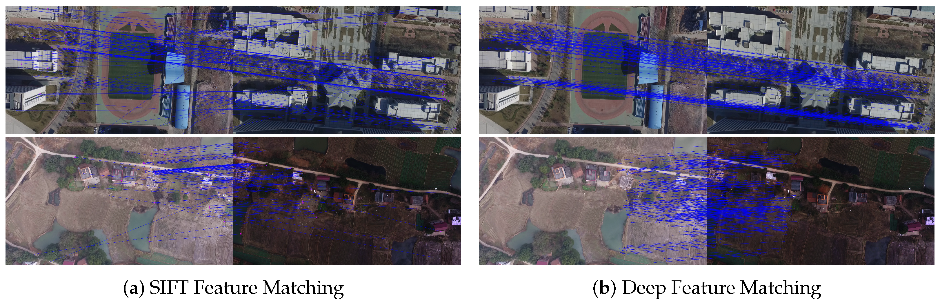
Similar to [22], the descriptors will be normalized by L2 as ${\widehat{d}}_{ij}=d_{ij}/{∥d_{ij}∥}_2$. Furthermore, we use Euclidean distance to compare descriptor vectors between serialized images. The feature maps are generated by fusing the output results of multiple neural network layers. In addition, the resolution of the feature image becomes one-quarter of the original image, which can detect more feature points and enhance the robustness. As we can see from Figure 2, SIFT features have unparalleled representational advantages over ordinary images. However, in the case of less feature texture of the target surface, or for the target with smooth edges, it cannot be accurately matched. D2-net uses a single convolutional neural network to simultaneously detect features and extract dense feature descriptors. By putting the detection into the later stage of processing, more stable and more robust feature point extraction can be obtained, especially for the morning and evening scenes and low-texture areas. Obviously, the feature matching results of D2-net are much better than SIFT under significant appearance differences caused by wide baseline.

In contrast to general SLAM algorithm, our joint feature descriptors-based covisibility cluster generation strategy can efficiently improve the accuracy of feature matching with excessively wide baseline, which will be more suitable for practical loop closure detection.

2.2. Serialized Dense Point Cloud Reconstruction

Constrained by covisibility cluster, our camera poses are optimized by using the “Bundle Fusion” strategy [23], and then the serialized SfM is achieved by bundle adjustment with optimized camera pose. Similar to the pipeline of OpenMVS [24], corresponding depth is then calculated and continuously refined by serialized PatchMatch until the complete point clouds are synthesized.

(1) Serialized Depth Estimation: Inspired by PatchMatch stereo matching [25], our serialization strategy is to estimate the depth constrained by covisibility cluster. The depth information of the current frame $K_i\in X_i^c$ can be compensated by multiple depth maps to reduce the errors caused by occlusion.

Different from OpenMVS, we integrate geometric consistency constraints between serialized images into cost aggregation to further improve the accuracy of depth estimation. The calculation of geometric consistency between the source image and the reference image is defined as the preprojection and post-projection error, ${\psi }_l^m=∥x_l-H_l^m{H}_l{x}_l∥$, where $H_l^m$ denotes the projective backward transformation from the source to the reference image.

(2) Dense Point Cloud Fusion in Sequential: In this part, depth map of the current frame could be merged to the existing point cloud scene. However, merging depth map directly may contain lots of redundancies because different depth maps may have common coverage of the scene, especially for neighboring images in covisibility cluster.

In order to remove these redundancies, the depth map of current frame is further reduced by the neighboring depth map. Let $d\left(x\right)$ be the current depth information and $\lambda \left(x\right)$ be the depth value of the current image reprojected to another image. If $d\left(x\right)$ and $\lambda \left(x\right)$ are close enough,

$$\begin{array}{c}\hfill \frac{\left|d\left(x\right)-\lambda \left(x\right)\right|}{\lambda \left(x\right)}<\tau \end{array}$$

(3)

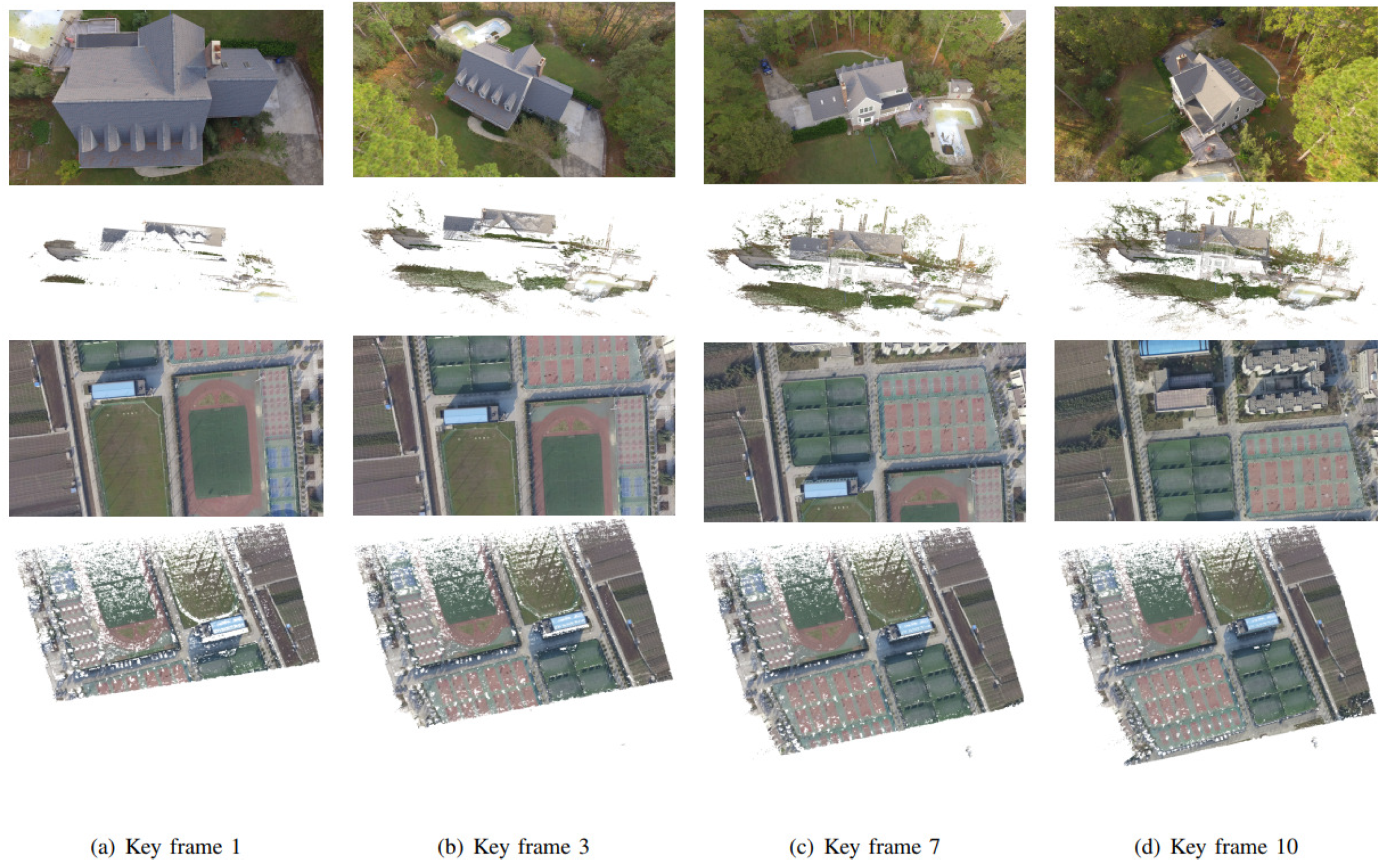
then it is considered as a reliable 3D point and the depth value of the corresponding pixel is retained; otherwise, it is removed. Finally, the optimized depth image will be reprojected to obtain a good quality sub-cloud and merged into previously generated point cloud. The visual results of our serialized reconstruction process are given in Figure 3.

3. Experiment and Evaluation

In order to demonstrate the performance of our algorithm and facilitate future research, we designed a dataset with five nature scenes (scene 1: residential area, scene 2: urban architecture, scene 3: rural areas, scene 4: mountains, scene 5: campus), which uses commercial software PhotoScan (v1.2.5) and Pix4D (V4.3.9) as the benchmark. Among them, scenes 4 and 5 are superscale aerial videos, which cover more than 1000 frames at the square kilometer level. The data had rich textured areas (buildings), repeated textured areas (pavement and plants) and untextured areas (water). At the same time, there are different time periods of data acquisition; the image illumination changes greatly. All of these scenarios are applicable to 3D reconstruction, and each presents its own unique challenges. It should be noted that the original five nature scenes are historical data collected before our work. At that time, we did not consider using LIDAR so it was very difficult to add the corresponding LIDAR data as the ground truth. Three well-known 3D point cloud reconstruction systems (PMVS, COLMAP and OpenMVS) as competitive targets are compared with our methods (Please refer to Table 1). Next, we analyze the experimental results from three aspects:

(1) Performance of Feature Extraction and Matching: In order to achieve robust feature extraction and matching both in the temporal and spatial covisibility cluster, we utilize SIFT features on the temporal series and VGG-16-based convolutional neural network features on the spatial series, respectively. As we can see from the first row of Table 2, the speed of our joint feature extraction and matching is the fastest among all the compared methods.

Furthermore, we analyze the time complexity of the feature matching strategy. PMVS, COLMAP, OpenMVS and PhotoScan adopt the global unordered matching strategy; the complexity is $O\left(n^2\right)$. We only detect the relationship of feature matching in a fixed window, so the time complexity is only $O\left(cn\right)$.

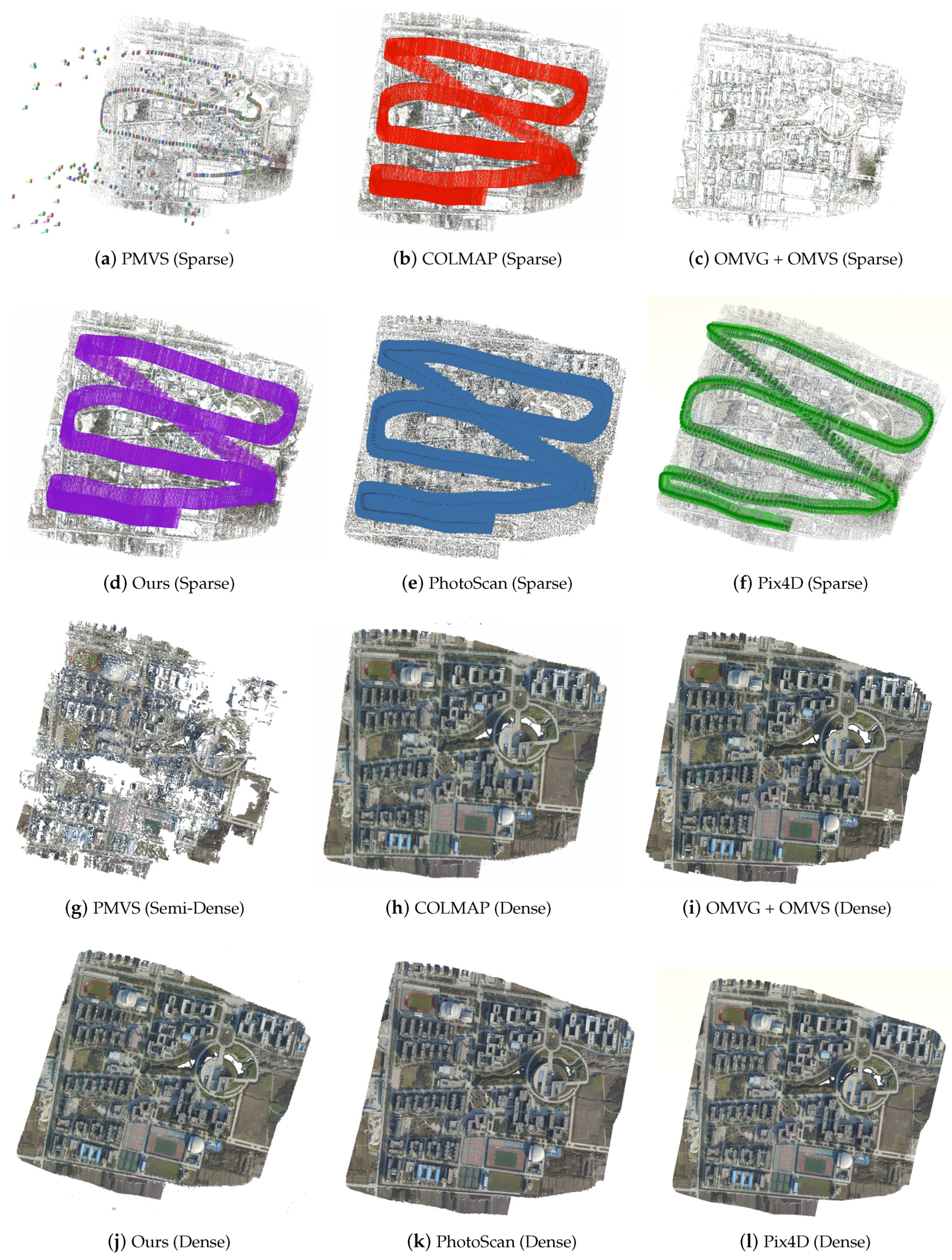
(2) Accuracy and Visual Effect of Point Cloud: Our serialized dense point cloud reconstruction framework utilizes the GPU parallel acceleration strategy to balance the reconstruction accuracy and efficiency for a large-scale complex aerial scene, which is suitable for the rapid presentation and analysis of practical applications. Figure 4a,f and Figure (a) in Table 2 declare that the reconstruction quality of PMVS (semi-dense) is the worst. The estimated camera poses drift seriously. Meanwhile, a lot of deformation and holes appear in the point cloud. Our method can achieve a competitive quality in sparse and dense reconstructions with PhotoScan and COLMAP, as Figure 4 shows (more visual results of our method can be seen in Figure 5). For the accuracy evaluation, we randomly selected several ROIs of the current cloud, searched their nearest points in the references and computed their MD (mean euclidean distance) and SD (standard deviation). As we can see in Table 1, the accuracy of our method is competitive with COLMAP. In order to better prove the accuracy and advanced degree of our method in the dense point cloud reconstruction of natural aerial scenes, in particular, we compared one of the current SOTA methods RTSfM [26] for 3D dense point cloud reconstruction. It proposed an efficient and high-precision solution for high-frequency video and large baseline high-resolution aerial images. Compared with the most advanced 3D reconstruction methods at present, this system can provide a large-scale high-quality dense point cloud model in real time. At the same time, in order to illustrate our performance, the test data were selected using extremely large scale aerial videos (scene 4 and scene 5). The shooting time span of these data is large and the texture is diverse with occlusions, which will bring great challenges for dense 3D point cloud reconstruction. As we can see in Table 3, our method has a similar performance to the point cloud results produced by RTSfM. It shows that the accuracy of our reconstruction is competitive with the existing SOTA methods.

(3) Comprehensive Performance of Reconstruction: We evaluate each algorithm by referring to the comprehensive comparison of the time complexity (Table 2) and reconstruction accuracy (Table 1).

Table 1. The Accuracy Comparison of 3D Dense Point Cloud Reconstruction (measurement unit of MD and SD is meter).

(A) Compared with PhotoScan (Dense)
Dataset	PMVS (Semi-Dense)		COLMAP (Dense)		OpenMVG +OpenMVS (Dense)		PhotoScan (Medium Dense)		Ours (Dense)
	MD	SD	MD	SD	MD	SD	MD	SD	MD	SD
Scene 1	0.672	1.398	0.119	0.112	0.385	0.291	0.037	0.032	0.191	0.135
Scene 2	6.824	4.589	0.141	0.176	1.153	0.210	0.261	0.261	0.278	0.235
Scene 3	1.225	0.918	0.355	0.256	0.060	0.062	0.164	0.164	0.328	0.268
(B) Compared with Pix4D (Dense)
Dataset	PMVS (Semi-Dense)		COLMAP (Dense)		OpenMVG +OpenMVS (Dense)		PhotoScan (Medium Dense)		Ours (Dense)
	MD	SD	MD	SD	MD	SD	MD	SD	MD	SD
Scene 1	11.129	15.853	1.405	1.441	1.530	1.063	1.648	1.283	1.701	1.460
Scene 2	24.746	22.858	0.533	0.439	0.227	0.248	1.319	1.277	1.232	1.029
Scene 3	4.688	4.289	0.981	0.478	0.216	0.237	0.942	0.836	0.882	0.578

Table 1. The Accuracy Comparison of 3D Dense Point Cloud Reconstruction (measurement unit of MD and SD is meter).

(A) Compared with PhotoScan (Dense)
Dataset	PMVS (Semi-Dense)		COLMAP (Dense)		OpenMVG +OpenMVS (Dense)		PhotoScan (Medium Dense)		Ours (Dense)
	MD	SD	MD	SD	MD	SD	MD	SD	MD	SD
Scene 1	0.672	1.398	0.119	0.112	0.385	0.291	0.037	0.032	0.191	0.135
Scene 2	6.824	4.589	0.141	0.176	1.153	0.210	0.261	0.261	0.278	0.235
Scene 3	1.225	0.918	0.355	0.256	0.060	0.062	0.164	0.164	0.328	0.268
(B) Compared with Pix4D (Dense)
Dataset	PMVS (Semi-Dense)		COLMAP (Dense)		OpenMVG +OpenMVS (Dense)		PhotoScan (Medium Dense)		Ours (Dense)
	MD	SD	MD	SD	MD	SD	MD	SD	MD	SD
Scene 1	11.129	15.853	1.405	1.441	1.530	1.063	1.648	1.283	1.701	1.460
Scene 2	24.746	22.858	0.533	0.439	0.227	0.248	1.319	1.277	1.232	1.029
Scene 3	4.688	4.289	0.981	0.478	0.216	0.237	0.942	0.836	0.882	0.578

Table 2. The Comparison of Time Complexity. (Dense and medium dense (defined by PhotoScan software) point clouds are usually used for 3D reconstruction tasks requiring demanding precision, and the data scale is at the level of ten million points per frame. Semi-dense point clouds are commonly used in automatic drive high-precision maps with data scale of millions of points per frame).

Methods	PMVS (Semi-Dense)	COLMAP (Dense)	OpenMVG +OpenMVS (Dense)	PhotoScan (Medium Dense)	Ours (Dense)	PhotoScan (Dense)	Pix4D (Dense)
Feature Extraction and Matching	95.0 min	47.92 min	215 min	60 min	19.58 min	62 min	33 min
Feature Matching Complexity	$O\left(n^2\right)$	$O\left(n^2\right)$	$O\left(n^2\right)$	$O\left(n^2\right)$	$\mathit{O}\left(\mathit{cn}\right)$	$O\left(n^2\right)$	$O\left(n^2\right)$
Dense Reconstruction Time	20.0 min	328.36 min	148 min	153 min	224 min	1494 min	263 min
Total Dense Points	1,182,982	24,261,818	29,982,611	33,123,377	23,881,812	52,442,997	4,164,972
Partial Detail (Scene 1)	(a)	(b)	(c)	(d)	(e)	(f)	(g)

Table 2. The Comparison of Time Complexity. (Dense and medium dense (defined by PhotoScan software) point clouds are usually used for 3D reconstruction tasks requiring demanding precision, and the data scale is at the level of ten million points per frame. Semi-dense point clouds are commonly used in automatic drive high-precision maps with data scale of millions of points per frame).

Methods	PMVS (Semi-Dense)	COLMAP (Dense)	OpenMVG +OpenMVS (Dense)	PhotoScan (Medium Dense)	Ours (Dense)	PhotoScan (Dense)	Pix4D (Dense)
Feature Extraction and Matching	95.0 min	47.92 min	215 min	60 min	19.58 min	62 min	33 min
Feature Matching Complexity	$O\left(n^2\right)$	$O\left(n^2\right)$	$O\left(n^2\right)$	$O\left(n^2\right)$	$\mathit{O}\left(\mathit{cn}\right)$	$O\left(n^2\right)$	$O\left(n^2\right)$
Dense Reconstruction Time	20.0 min	328.36 min	148 min	153 min	224 min	1494 min	263 min
Total Dense Points	1,182,982	24,261,818	29,982,611	33,123,377	23,881,812	52,442,997	4,164,972
Partial Detail (Scene 1)	(a)	(b)	(c)	(d)	(e)	(f)	(g)

Table 3. The accuracy evaluation between RTSfM and our method by using new data. (The extra data from scene 4 and scene 5 are used for SOTA competition. Ground truth is set as PhotoScan (dense) and the measurement unit of MD and SD is meter).

Method	RTSfM [26]		Ours
	MD	SD	MD	SD
Scene 4	0.460	0.441	0.425	0.431
Scene 5	0.721	0.816	0.906	0.914

Table 3. The accuracy evaluation between RTSfM and our method by using new data. (The extra data from scene 4 and scene 5 are used for SOTA competition. Ground truth is set as PhotoScan (dense) and the measurement unit of MD and SD is meter).

Method	RTSfM [26]		Ours
	MD	SD	MD	SD
Scene 4	0.460	0.441	0.425	0.431
Scene 5	0.721	0.816	0.906	0.914

PMVS is the fastest method. However, it can only generate semi-dense point clouds (1,182,982 points). Table 2(a) shows the building structure generated by PMVS is seriously lacking in details. Despite its high speed, it is not suitable for high-precision dense point cloud reconstruction.

Nearly 26 h of running time of PhotoScan is unacceptable for practical applications. The medium density of PhotoScan is relatively fast, but the outer contour of the generated building is seriously deformed (see Table 2(d)).

It is clear that the efficiency of rebuilding with either method increases with the number of points. The influence of different reconstruction densities on the running time is obvious. However, the total number of points generated by our method is almost half that of PhotoScan, and our result still maintains similar good edge details (see Table 2(e)) and accuracy with COLMAP (see Table 1). Meanwhile, our computation speed is nearly $6.7$ times faster than PhotoScan and $1.5$ times faster than COLMAP. Furthermore, OpenMVS is time-consuming in relation to feature computation, which is 11 times slower than our method, and the number of points generated by the Pix4D method is much less than ours. Considering the comprehensive performance, our algorithm is very competitive in practicability.

Figure 4. Visual comparison (Scene 1) of point cloud reconstruction results between our method and other 5 existing outstanding methods. (The result of PhotoScan and Pix4D as the benchmark).

Figure 4. Visual comparison (Scene 1) of point cloud reconstruction results between our method and other 5 existing outstanding methods. (The result of PhotoScan and Pix4D as the benchmark).

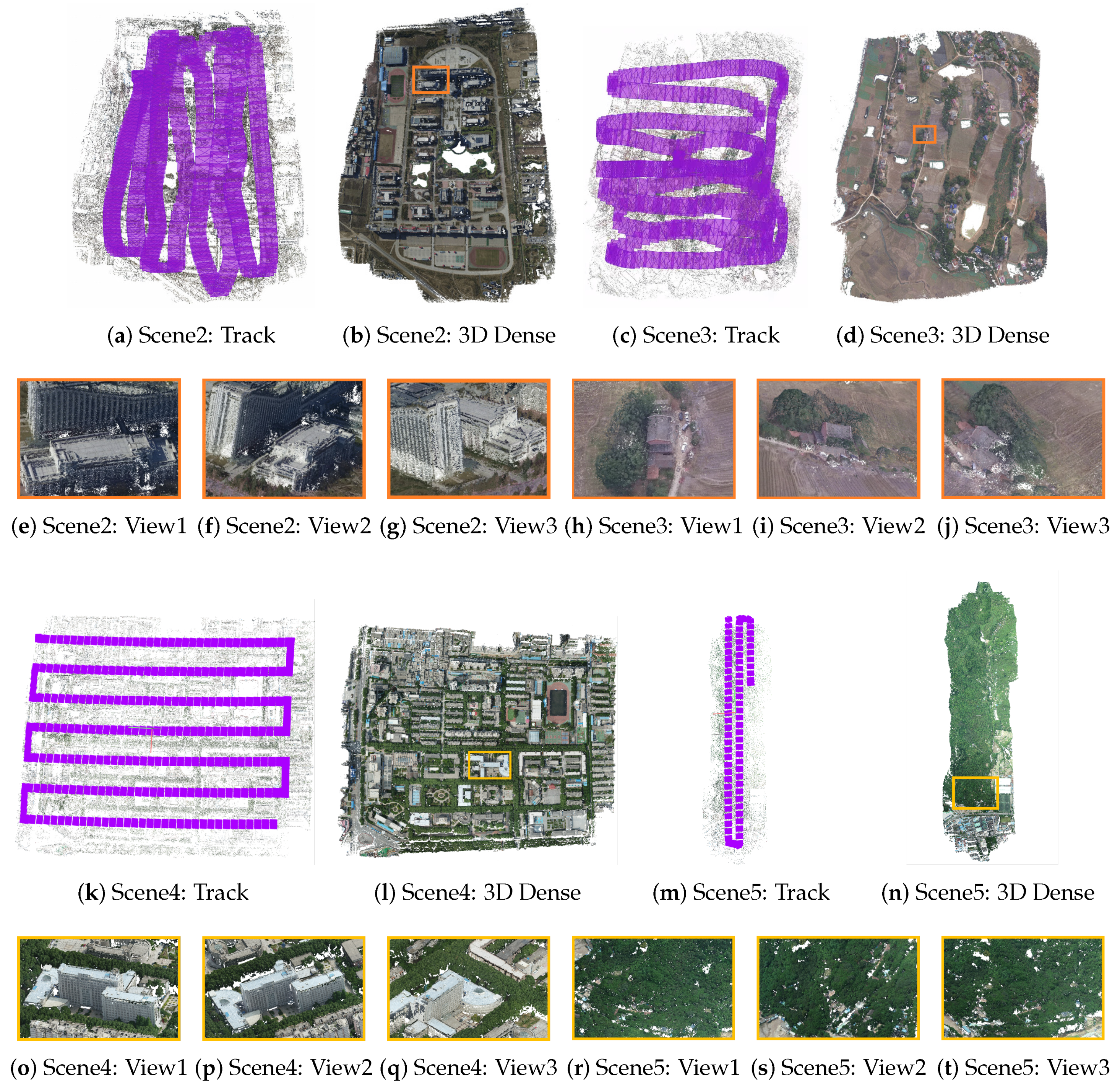
Figure 5. Various Reconstructions of Our Methods. (We enlarge the point cloud area of buildings with yellow bounding box).

Figure 5. Various Reconstructions of Our Methods. (We enlarge the point cloud area of buildings with yellow bounding box).

4. Conclusions

In this paper, we presented a serialized dense point cloud reconstruction for aerial video sequences by taking both high accuracy and efficiency into account. Firstly, we jointly utilized traditional feature descriptors and deep feature descriptors to apply a temporal and spatial correlation search to accelerate the feature matching and improve the accuracy of the pose estimation. Then, we provided our serialized structure-from-motion (SfM) and dense point cloud reconstruction framework. Finally, we collected a public aerial sequences dataset with referable ground truth for the dense point cloud reconstruction evaluation. In future work, we will focus on expanding the public dataset and the algorithm performance enhancement.