Article

Evaluating Carbon Sink Potential of Forest Ecosystems under Different Climate Change Scenarios in Yunnan, Southwest China

State Key Laboratory of Earth Surface Processes and Resource Ecology, Faculty of Geographical Science, Beijing Normal University, Beijing 100875, China
*
Author to whom correspondence should be addressed.
Remote Sens. 2023, 15(5), 1442; https://doi.org/10.3390/rs15051442
Submission received: 8 February 2023 / Revised: 2 March 2023 / Accepted: 3 March 2023 / Published: 4 March 2023
(This article belongs to the Special Issue Forest Biomass/Carbon Monitoring towards Carbon Neutrality)

Abstract

:
Nature-based Solutions (NbS) can undoubtedly play a significant role in carbon neutrality strategy. Forests are a major part of the carbon budget in terrestrial ecosystems. The possible response of the carbon balance of southwestern forests to different climate change scenarios was investigated through a series of simulations using the forest ecosystem carbon budget model for China (FORCCHN), which clearly represents the influence of climate factors on forest carbon sequestration. Driven by downscaled global climate model (GCM) data, the FORCCHN evaluates the carbon sink potential of southwestern forest ecosystems under different shared socioeconomic pathways (SSPs). The results indicate that, first, gross primary productivity (GPP), ecosystem respiration (ER) and net primary productivity (NPP) of forest ecosystems are expected to increase from 2020 to 2060. Forest ecosystems will maintain a carbon sink, but net ecosystem productivity (NEP) will peak and begin to decline in the 2030s. Second, not only is the NEP in the SSP1-2.6 scenario higher than in the other climate change scenarios for 2025–2035 and 2043–2058, but the coefficient of variation of the NEP is also narrower than in the other scenarios. Third, in terms of spatial distribution, the carbon sequestration potential of northwest and central Yunnan is significantly higher than that of other regions, with a slight upward trend in NEP in the future. Finally, GPP and ER are significantly positively correlated with temperature and insignificantly correlated with precipitation, and the increasing temperature will have a negative and unstable impact on forest carbon sinks. This study provides a scientific reference for implementing forest management strategies and achieving sustainable development.

1. Introduction

To tackle climate change and accelerate sustainable development, the Chinese government has set the strategic goals of peaking CO2 emissions by 2030 and achieving carbon neutrality by 2060 [1]. The carbon sink of terrestrial ecosystems in China (0.24 Pg C·yr−1) has significantly offset some of the carbon emissions from fossil fuel burning and land use change (10~40%) over the past decades [2]. From the perspective of sink enhancement, the Chinese government proposes strengthening ecological protection to consolidate the carbon sink capacity of natural ecosystems [3]. However, there are still great uncertainties in the future carbon sequestration potential of ecosystems.
Net ecosystem productivity (NEP) is the difference between gross primary productivity (GPP) and ecosystem respiration (ER) [2]. NEP is commonly used as a measure of carbon sinks in terrestrial ecosystems. If the NEP is positive, the ecosystem is a carbon sink, and if not, it is a carbon source. Regional terrestrial ecosystem carbon balance estimation methods include field inventories [4,5,6,7,8], terrestrial ecosystem models [9,10,11,12], atmospheric inversion methods [13,14,15,16], and upscaling methods of flux observation data [17,18,19,20,21], but there are some differences in the estimation results of different methods. In particular, ecosystem modeling has become an effective tool for understanding and evaluating terrestrial carbon cycles at the sample point at both regional and global scales [22,23,24,25,26,27]. It can quantitatively distinguish the contributions of different drivers to changes and accurately evaluate the impacts of future climate change on carbon sinks.
The forest ecosystem carbon budget model for China (FORCCHN) is a self-developed patch model based on individual growth processes and meteorological data. There are four main characteristics: (1) the cycle and transformation processes of carbon, nitrogen, and water at different interfaces of atmosphere–plant–soil are organically combined; (2) the drivers of forest ecosystem carbon balance are not predetermined by the current climate and ecosystem statistical relationships but rather are based on individual physiological–ecological process mechanisms that are coupled; (3) the carbon flux of the forest is determined by the individual growth of the stand so that the carbon budget can be simulated more scientifically and reasonably; and (4) models can accurately elaborate woody biomass and are more advantageous in predicting the effect of climate factors on carbon fluxes. The model has been used to simulate the carbon balance of different types of forests in China and the world [28,29,30,31] and performs particularly well in capturing the temporal variability and magnitude of carbon fluxes in deciduous broadleaf and evergreen broadleaf forests. Therefore, the model is suitable for assessing the carbon sequestration potential of forest ecosystems.
Both ecosystem carbon conservation and sink enhancement are considered to be the greenest, most economical and scale-effective technology pathways [32]. In recent decades, forest ecosystems have contributed more than 80% of the annual average terrestrial carbon sink in China [7,33,34]. Yu et al. found that the spatial distribution pattern of carbon sequestration in China’s forests was high in the east and south and low in the west and north through ChinaFlux [19,35,36,37,38]. Moreover, the southwest region is confirmed to be one of the regions with the largest carbon sequestration capacity through various research tools, such as atmospheric inversion, flux observation, and ecological modeling [15,38,39,40]. In addition, the southwest forest region is the largest natural forest area and the implementation area of major forestry ecological projects in China, but there is a lack of research on the future carbon sequestration potential of this region.
The latest Coupled Model Intercomparison Project Phase 6 (CMIP6) provide a coordinated set of global climate model (GCM) simulations to understand how the Earth system responds to forcings and provide predictions for the future [41].The model data include different shared socioeconomic pathways (SSPs): the SSP1-2.6 scenario assumes a mean temperature below 2 °C for the model ensemble at the end of the 21st century, which represents a low level of atmospheric radiative forcing and socioeconomic vulnerability; the SSP2-4.5 scenario assumes a medium level of atmospheric radiative forcing and socioeconomic vulnerability; and the SSP5-8.5 scenario assumes the highest concentrations of greenhouse gas emissions, with low levels of science, technology and innovation, poor energy improvement conditions, and high energy demand [42]. Under the SSP1-2.6, SSP2-4.5, and SSP5-8.5 scenarios, the average surface temperature in China is projected to increase by 1.31 °C, 1.32 °C, and 1.45 °C in the near term (2021–2040) and by 1.75 °C, 2.06 °C, and 2.66 °C in the medium term (2041–2060), respectively [43,44]. At present, there is still insufficient research on carbon sinks in China’s terrestrial ecosystems under different SSPs in the future [2,45,46,47,48]. The regional carbon sink potential and climate risk need to be urgently clarified, and in particular the contribution of future climate change to the carbon sink potential of regional forest ecosystems needs to be quantified.
Therefore, this paper combined meteorological data with high spatial and temporal resolutions obtained by a GCM through downscaling methods to quantify carbon sinks in southwest forest areas under different climate change scenarios in the next 40 years. This research analyzes the relationship between carbon fluxes and meteorological factors. Optimization suggestions for forest area management are proposed to serve the national carbon neutrality strategy.

2. Materials and Methods
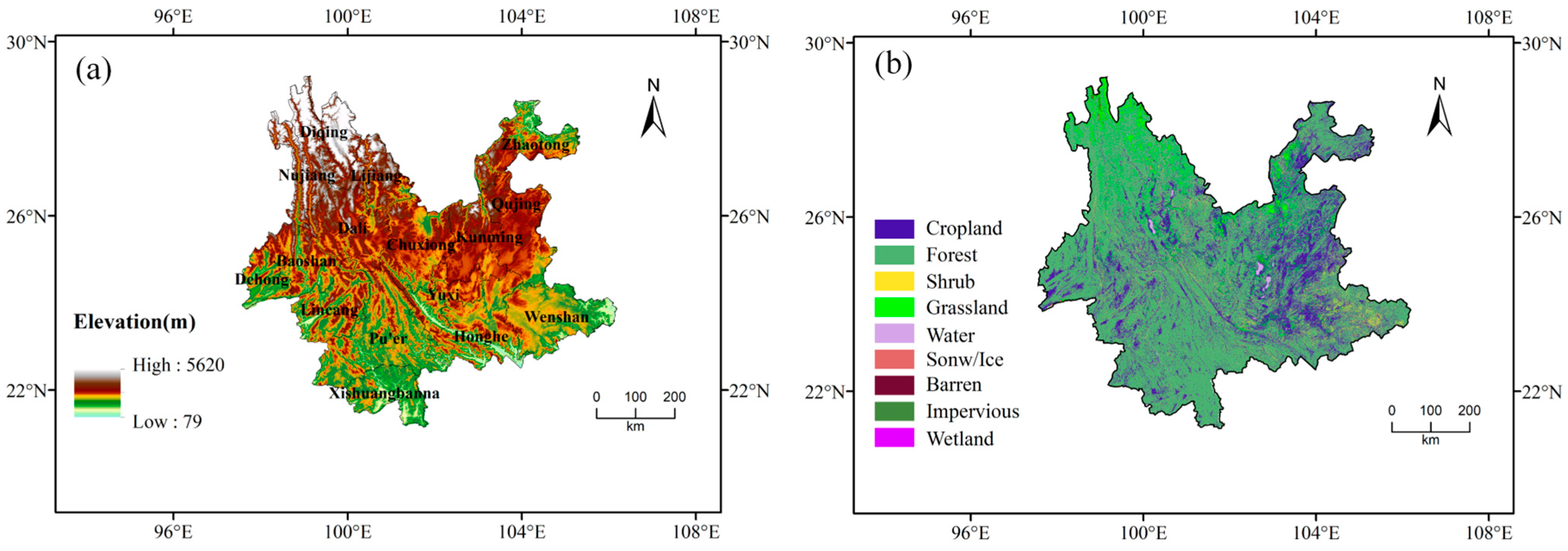
2.1. Study Area

Yunnan Province (21°8′32″~29°15′8″N, 97°31′39″~6°11′47″E) is located on the southwest border of China, adjacent to Myanmar, Vietnam, and Laos, with a total area of approximately 39.4 × 10⁴ km2 [49]. Yunnan Province has a special geographical location and complex topography, with stretches of plateaus in the east and mountains and rivers in the west, and the terrain is high in the northwest and low in the southeast, with an obvious stepwise descent (Figure 1a). There is a very large difference in altitude, with a relative height difference of 6664 m [50]. Climatically, the study area has a subtropical and tropical monsoon climate, which belongs to the intersection of three famous climate zones: South Asian monsoon, East Asian monsoon, and the Qinghai-Tibet Plateau [51], with an annual temperature difference of 10 °C to 12 °C. Precipitation is unevenly distributed seasonally and geographically, with 85% of precipitation concentrated in the wet season from May to October [52]. The highest annual precipitation in the province is 2200 to 2700 mm, while the lowest is only 584 mm. The diverse climate types and unique geographical environment have nurtured rich forest resources, and more than 50% of the area is covered by forests [53] (Figure 1b), which consist of evergreen broad-leaved forests, evergreen coniferous forests, and mixed forests [54]. The soils are brick red loam and red loam.

2.2. FORCCHN Model Description

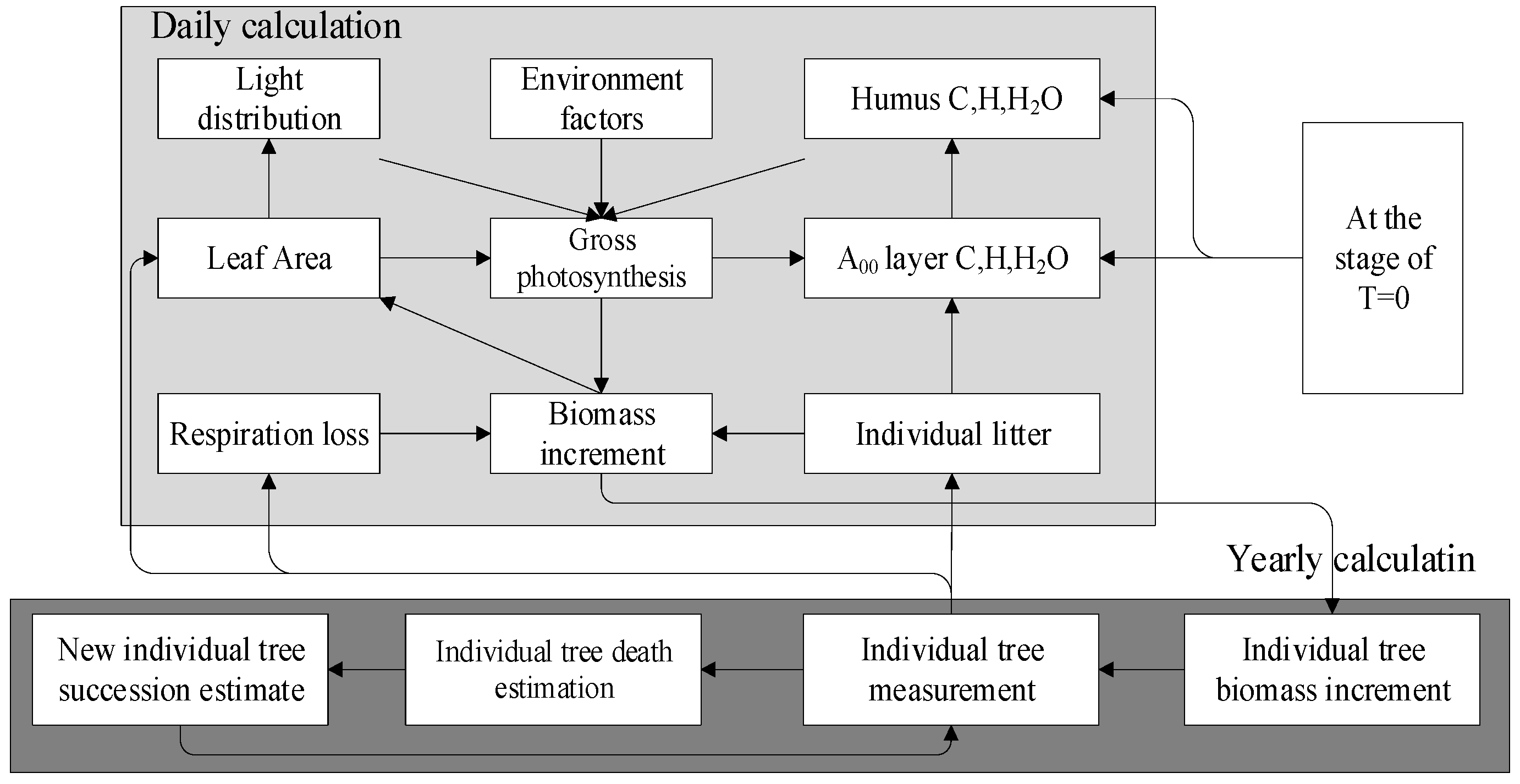
2.2.1. Structure and Characteristics of the Model

FORCCHN is an individual-based carbon cycle model driven by daily meteorological data that simulates the carbon dynamics of forest ecosystems at the plot scale (~600 m2) by coupling soil carbon (C) pools [31] and runs in daily and annual time steps (Figure 2). The model assumes a relative balance of carbon, nitrogen (N), and water in the atmosphere–soil–forest system (Table 1). The daily C and N module of each tree includes total photosynthesis, maintenance respiration, growth respiration, photosynthetic product allocation, and litter. This model uses the photosynthate buffer pool to reduce tree death caused by climate extremes. The model allocates the daily net photosynthetic products to leaf and fine root growth and litter, while the rest are stored in the so-called “buffer carbon pool” (BCP). At the end of the year, the accumulated BCP is used primarily to support growth in canopy height and diameter at breast height (DBH), as well as coarse woody debris production (CWD). Note that trees are considered dead when there is not enough carbon for leaf production; the C, N, xylem, and litter contained in dead trees would be fully transferred to the soil pool on the last day of each year and continue to participate in new C and N cycles in the following year [55]. The FORCCHN of soil C and N dynamics is based on an improved CENTURE model [56,57]. The CENTURY model has good applicability in Chinese terrestrial ecosystems [58,59,60]. In short, the model consists of woody litter pools, aboveground and belowground litter pools, and three soil organic matter pools (active, slow, and inert), with their respective decomposition rates. Table 2 lists the litter decomposition parameters in the model [56]. The model classifies individual trees according to the specific species or plant function type to which they belong, according to the needs of the simulation. The physiological, ecological, and morphological parameters of each tree plant function type are described in Table S1. As the simulation period of this study is short, less than 80 years, it is assumed that tree regeneration will not occur. In addition, the model assumed constant forest distribution and area.

2.2.2. The Main Equations of the Model

The gross primary productivity of an individual tree is given by the equation:
G P P i = min ( G P P M i × f c × f d r y × f T , R c / n × S n )
where GPPi is the daily gross primary productivity of individual trees; GPPMi is the maximal daily gross primary productivity of individual trees; and fc, fdry, fT, and Rc/n × Sn represent the effects of carbon dioxide, water, temperature, and soil available nitrogen on GPP, respectively. Sn is the soil available nitrogen, and Rc/n is the C/N ratio parameter of the assimilation.
G P P M i = 2 × A m j × D l K l j × ln 1 + 1 + K l j × S l j × P A R i A m j 1 + 1 + K l j × S l j × P A R i × exp ( K l j × L A I i ) A m j
where Dl (daylength) is the possible sunshine duration (h), PARi is the noon canopy photosynthetically active radiation of the individual tree (Wm−2), and LAIi is the leaf area index of the ith tree. For the ith individual in the jth plant functional type, Amj, Klj, and Slj represent the maximal photosynthesis [kgC/(m−2·h−1)], the extinction coefficient, and the initial slope of light intensity and photosynthesis [kgC/(m2·h))/(W·m−2)], respectively.
f c ( C s ) = 1 + C s C 0 C s + 2 C 0
where Cs is the CO2 concentration of the simulation year, C0 is the CO2 reference concentration, and the atmospheric CO2 concentration was approximately 410 ppm in 2019, according to NASA observations [61,62]; therefore, C0 was set at 410 ppm.
f ( s w , r h ) = { min [ 1 , s w F C + max ( r h 0.5 , 0.1 ) ] d r y } 0.5
where sw is the soil water content (cm), FC is the field capacity (cm), rh is the air relative humidity, and dry is the individual’s capability of enduring drought, which ranges from 0 to 1.
f T ( T ) = ( T max T T max T o p t ) T max T o p t T max T min × ( T T min T o p t T min ) T o p t T min T max T min
where Topt is the photosynthetic optimum temperature (°C), Tmax is the photosynthetic maximum temperature (°C), Tmin is the photosynthetic minimum temperature (°C), and T is the average daily temperature of the day (°C).
The autotrophic respiration of each plant includes maintenance respiration and growth respiration. The formula for maintenance respiration is expressed as follows:
R M i k = t r e s p × r k C i k
where RMik is the daily maintenance respiration of the individual tree (kgC·d−1); rk is the relative respiration rate of leaves, branches, stems, main roots, and fine roots at a temperature of 15 °C (1/d); and Cik is the reservoir volume of the corresponding carbon pool (kgC); when k is for leaves and fine roots, the corresponding Cik is the content or fine root content, and when k is for stem or main root, the corresponding Cik is the sapwood content (kgC).
R G i = t r e s p × r g × ( G P P i R M i k )
where RGi is the daily growth respiration of i-the individual tree (kgC·d−1) [63] and rg is the growth respiration coefficient, usually 0.16–0.30, and was set to 0.25 in this model [30,31,64,65].
In Equations (6) and (7), tresp represents the effect of air temperature on plant respiration, and this value is computed as follows:
t r e s p = t r e s p D + t r e s p N
t r e s p D = D l 24 × e ln ( t g D ) 10 × ( T E M D 15 )
t g D = 2 × e 0.009 × ( T E M D 15 )
t r e s p N = 24 D l 24 × e ln ( t g N ) 10 × ( T E M N 15 )
t g N = 2.2 × e 0.009 × ( T E M N 15 )
where trespD and trespN represent the effect of daytime air temperature and nighttime air temperature on plant respiration, respectively, TEMD is the daytime air temperature (°C), TEMN is the nighttime air temperature (°C), and Dl is the possible sunshine duration for each day (h).

2.3. Model Driving Data

2.3.1. Meteorological Data

The maximum temperature (K), minimum temperature (K), mean temperature (K), precipitation (kg·m−2·s−1),wind speed (ms−1), relative humidity (%), shortwave radiation (W m−2), and pressure (Pa) were all from the GFDL-ESM4 product released by CIMP6 (https://esgf-node.llnl.gov/projects/cmip6/, accessed on 2 July 2022) [66] (Table 3), and because the model performs better in regional temperature and precipitation simulations in China, the monthly bias correction/spatial decomposition (BCSD) method was downscaled to generate day products with a horizontal resolution of 25 km [67] and then bilinearly interpolated to 10 km × 10 km, including meteorological variables under the SSP scenarios of SSP1-2.6, SSP2-4.5, and SSP5-8.5 scenarios from 2020 to 2060. The unit conversion formulae involved are as follows:
T F O R C C H N = T G F D L 273.15
where TFORCCHN and TGFDL represent the required temperature (°C) for the FORCCHN model and temperature (K) in the GFDL model, respectively.
P R F O R C C H N = P R G F D L × 86400
where PRFORCCHN and PRGFDL represent the required precipitation (mm) for the FORCCHN model and precipitation (kg·m−2·s−1) in the GFDL model, respectively.
P S F O R C C H N = P S G F D L / 100
where PSFORCCHN and PSGFDL represent the required air pressure (hPa) for the FORCCHN model and air pressure (Pa) in the GFDL model, respectively.

2.3.2. Soil Data

Soil data were available from the 1:100,000 digital soil property maps provided by the Nanjing Institute of Soil Research (http://www.issas.ac.cn/, accessed on 6 June 2022), Chinese Academy of Science (CAS), including soil sand content, soil meal content, soil clay content, soil bulk density, soil field water holding capacity, soil wilting coefficient, soil carbon density, soil nitrogen density, etc. [68]. Based on the properties of the soil profiles at different depths, a weighted sum of the soil property data was obtained for the corresponding grid points.

2.3.3. Vegetation Data

For each grid cell, a vegetation type map at a scale of 1:1,000,000 (approximately 1 km × 1 km) provided by the China Vegetation Map Editorial Committee, was used to determine its vegetation type [69,70,71]. MODIS C6 LAI data have a resolution of 500 m and a time series of 2000–2019, with improved accuracy through filtering algorithms and correction methods, and these data can be used for driving the model [72] (http://globalchange.bnu.edu.cn/research/laiv6, accessed on 2 October 2022).

2.3.4. CO2 Data and Elevation Data

Atmospheric CO2 concentration data from the historical period were available from the GLOBAL CLIMATE CHANGE Vital Signs of the Planet (https://climate.nasa.gov/vital-signs/carbon-dioxide/, accessed on 2 October 2022). We have set the 2020 CO2 concentration at 410 ppm, with future CO2 concentrations increasing at a rate of 1.5 ppm·yr−1. The digital elevation model (DEM) data were available from the Shuttle Radar Topography Mission (SRTM) released by NASA, with a spatial resolution of 1 km, and were resampled to 10 km in this study by ArcGIS 10.6.

2.4. Model Output

The FORCCHN model can output daily and annual-scale carbon flux data, and the main parameters include aboveground biomass, belowground biomass, gross primary productivity (GPP), net primary productivity (NPP), ecosystem respiration (ER), and net ecosystem productivity (NEP).

2.5. Model Validation

To evaluate the model’s performance in simulating carbon fluxes in forest ecosystems, the correlation coefficient (Corr), root mean square error (RMSE), and bias (Bias) of the simulation results with the observed values were used in this study. The equations are as follows:
C o r r = i = 1 n ( S i S ¯ ) ( O i O ¯ ) i = 1 n ( O i O ¯ ) 2 i = 1 n ( S i S ¯ ) 2
R M S E = 1 n i = 1 n ( S i O i ) 2
B i a s = 1 n i = 1 n ( S i O i )
where n is the year number and Si and Oi represent the simulated and observed carbon fluxes in the i-th year, respectively, and represent their averaged values.

3. Results

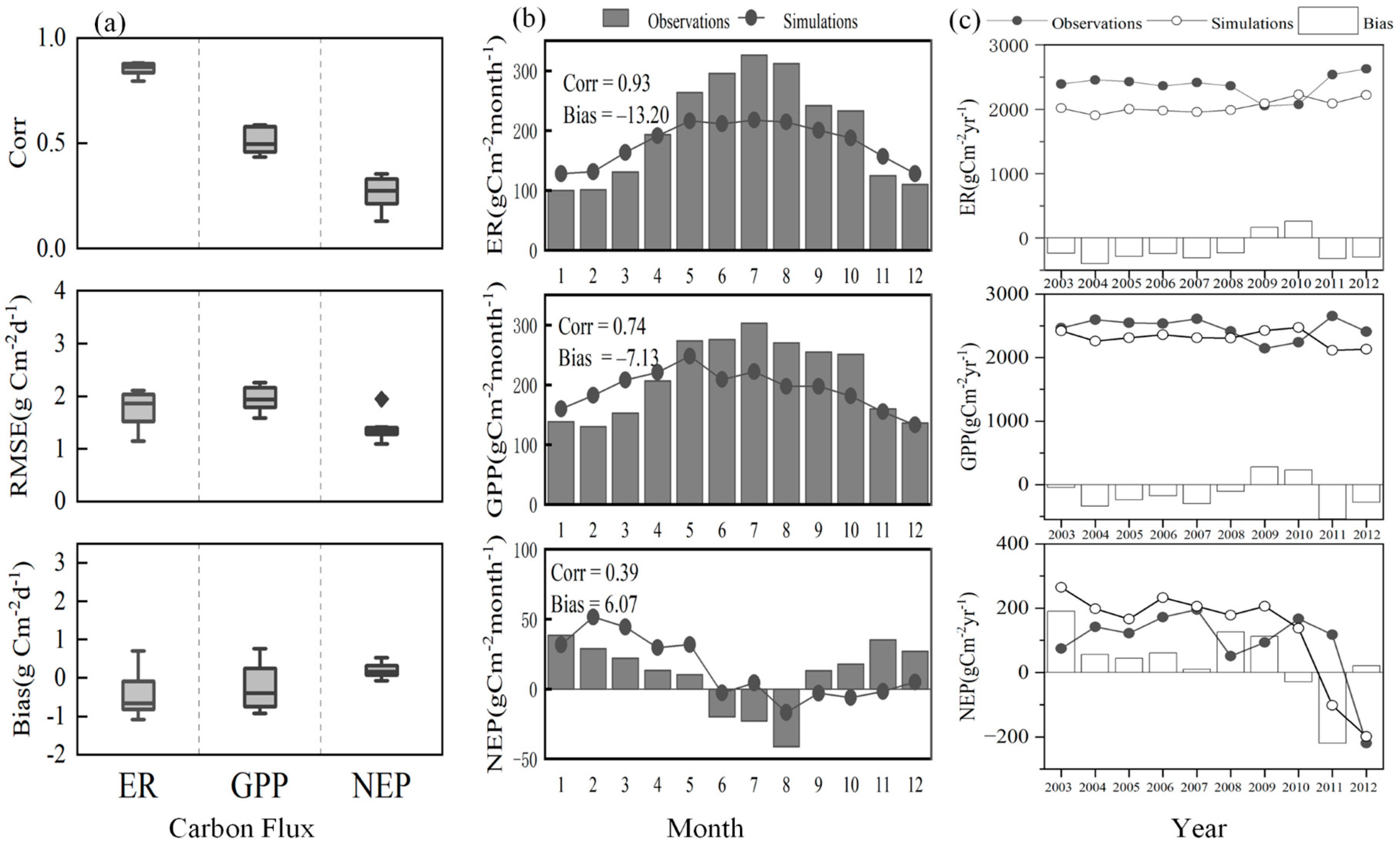
3.1. Simulation Performance

The eddy correlation technique is the most direct method used for measuring CO2 exchange and water and energy fluxes between the atmosphere and ecosystems and has been widely used in carbon cycle studies of terrestrial ecosystems. Carbon fluxes include ecosystem respiration (ER) and net ecosystem CO2 exchange (NEE). Net ecosystem productivity (NEP) and NEE have the same value and opposite sign. The observations at the Xishuang Banna station were derived from the ChinaFLUX ecosystem carbon and water fluxes and key meteorological elements dataset (http://www.chinaflux.org/, accessed on 16 May 2021), including daily and annual-scale flux data from 2003 to 2012.
Overall, the FORCCHN model reproduced the carbon fluxes of tropical seasonal rainforests on a daily scale (Figure 3a), with the maximum value of Corr occurring in ER (0.85), followed by GPP and NEP. FORCCHN slightly underestimated ER and GPP, and their corresponding mean deviations were −0.43 gC·m−2·d−1 and −0.21 gC·m−2·d−1, respectively, and the simulation results overestimated NEP (0.19 gC·m−2·d−1). The RMSEs of ER, GPP, and NEP were 1.77, 1.96, and 1.39 gC·m−2·d−1, respectively.
The simulated curves were very similar to the observed curve fluctuations, indicating that the model could reproduce the seasonal variation in tropical seasonal rainforests (Figure 3b). The model had a small underestimation of ER and GPP for tropical rainforests, and the simulated values were lower than the observed values by 6.83% and 3.56%, respectively. However, the model overestimated NEP by 3.50% above the observed value. It was able to reproduce the patterns of carbon sources (NEP < 0) and sinks (NEP > 0) in tropical seasonal rainforests throughout the year, with tropical rainforests being carbon sources from June to November and carbon sinks from December to May, which was consistent with in situ observations [73], but unfortunately, the model was numerically biased.
Analyzing the interannual variation and deviation of carbon fluxes in forest ecosystems from 2003 to 2012 (Figure 3c), the results showed that the FORCCHN model had the ability to simulate the trend of interannual variation in carbon fluxes in forest ecosystems, but there were differences in the magnitude of the values of the annual distance, and the average annual deviation rates of ER and GPP and NEP in tropical rainforests were −7.29%, 5.50%, and 14.90%, respectively.

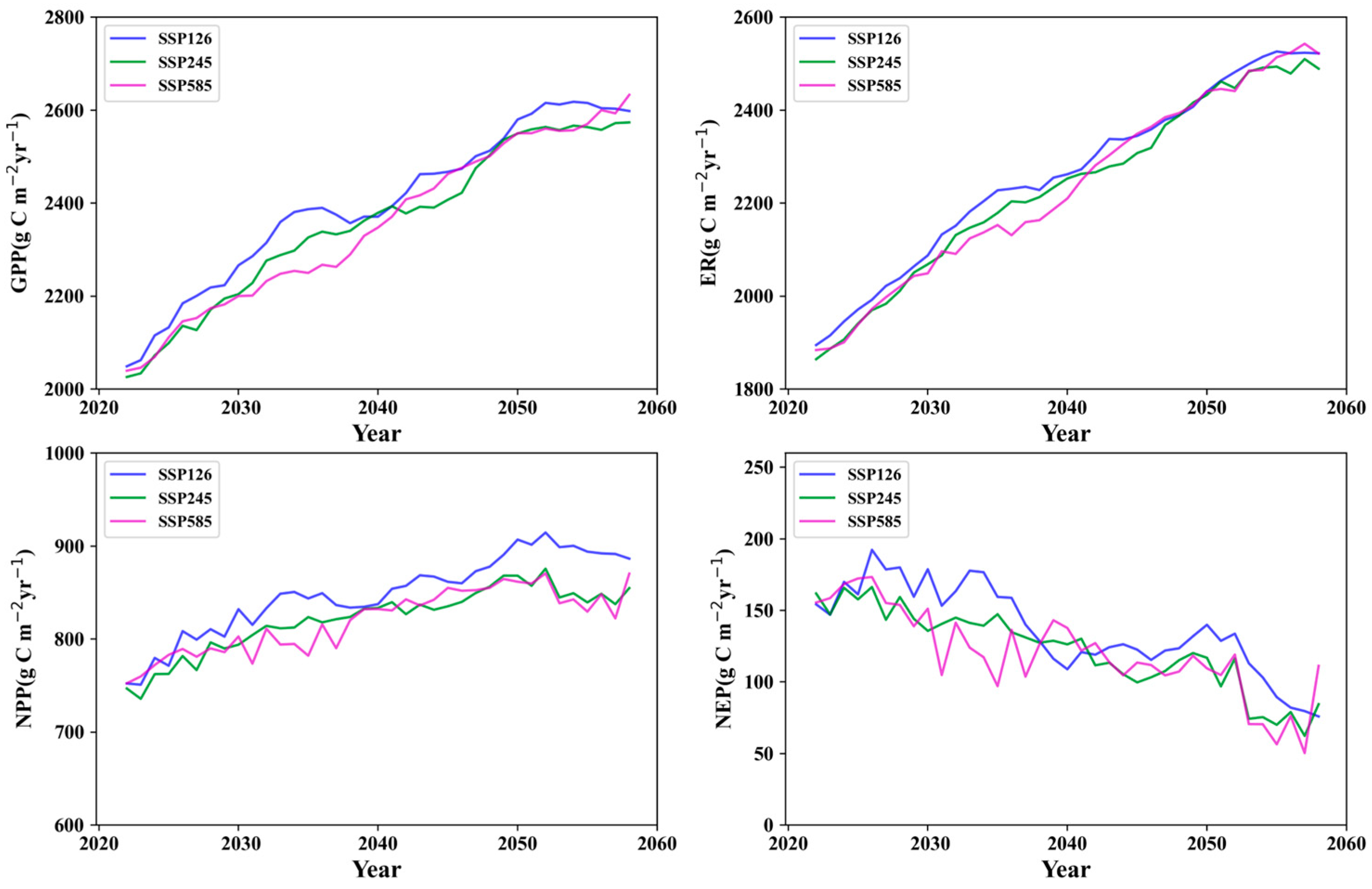
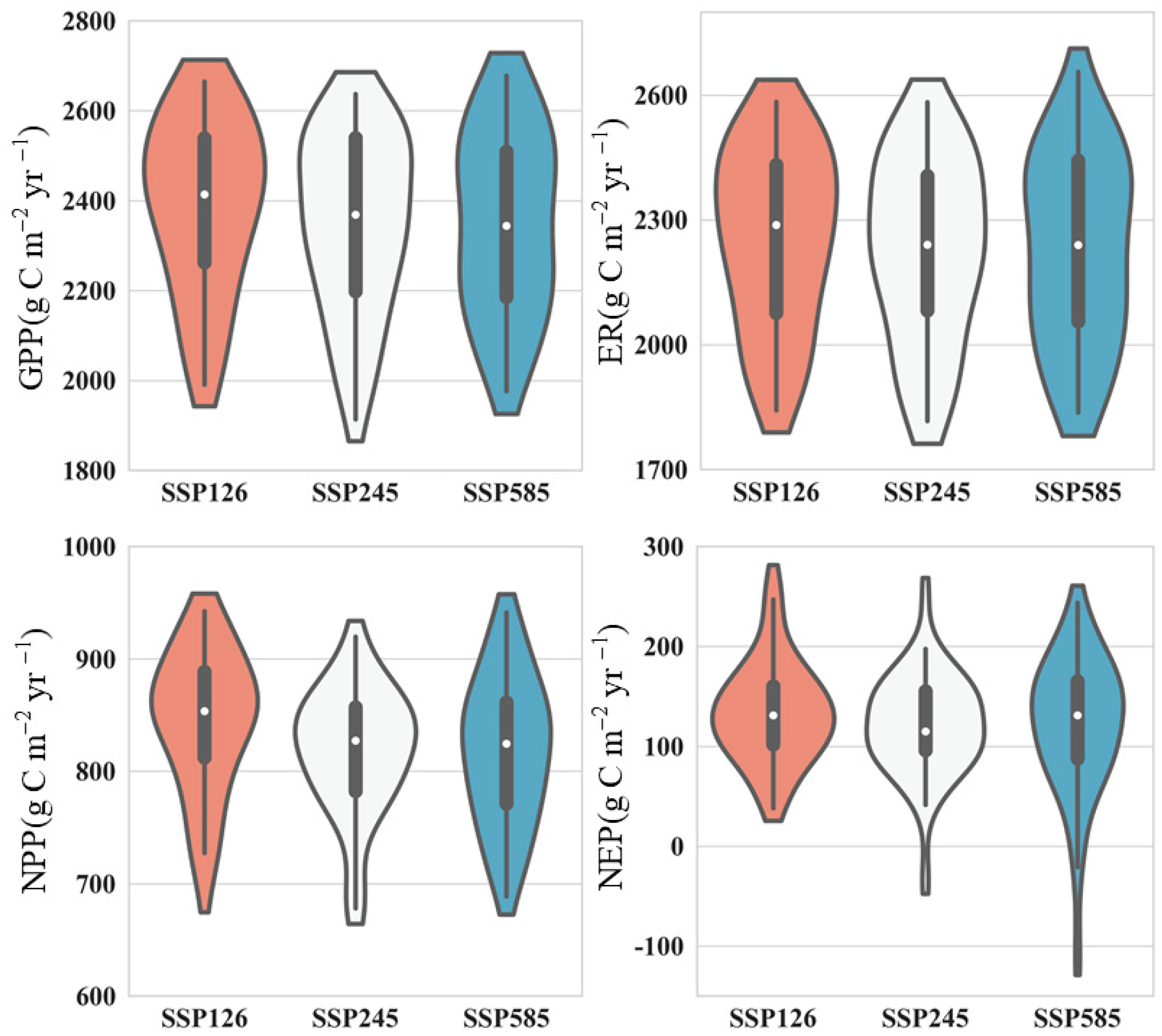
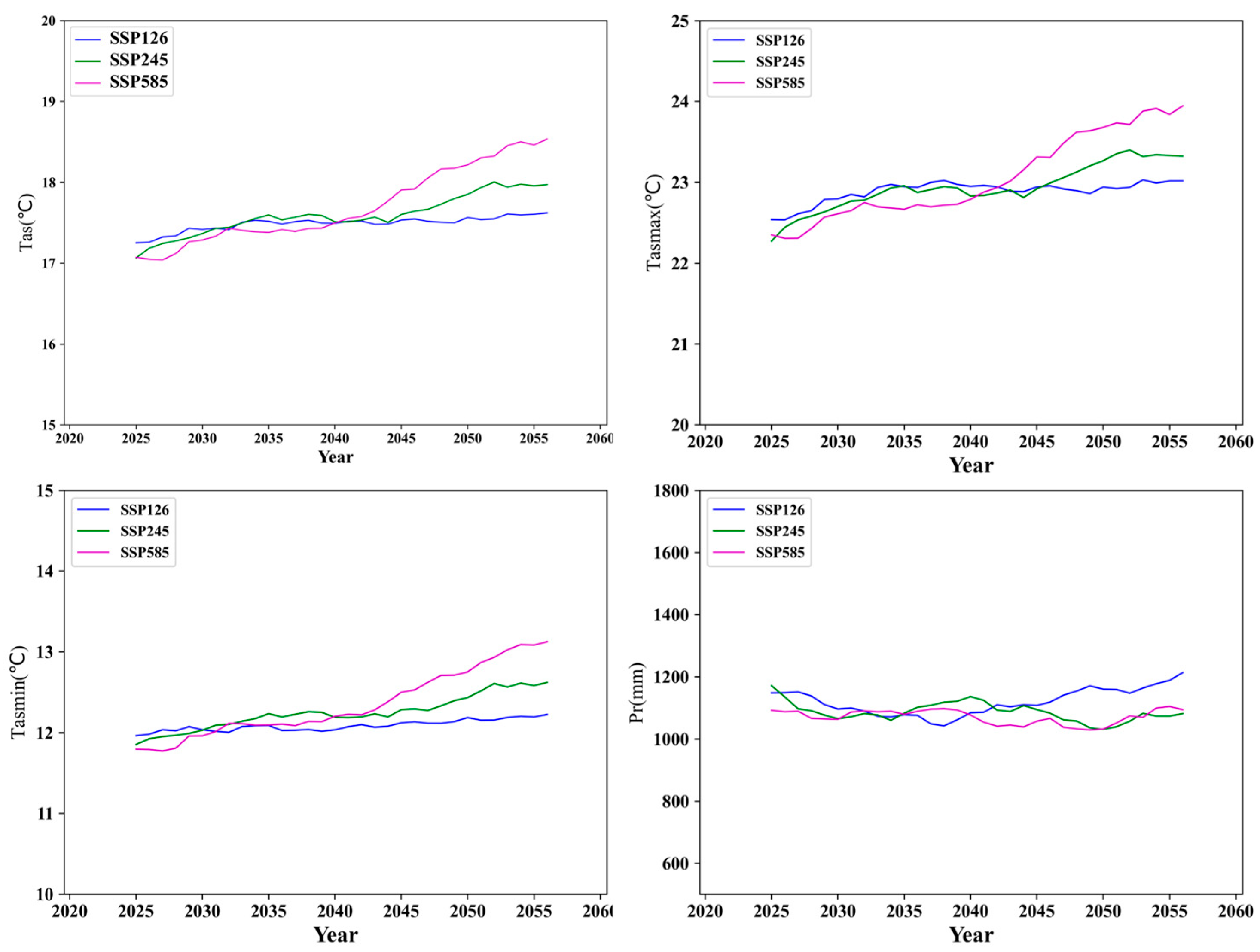
3.2. Interannual Variations in Carbon Fluxes

By simulating the forest carbon fluxes in Yunnan Province from 2020 to 2060, we observe that the annual means of GPP were 2388.76, 2348.97, and 2344.50 gCm−2·yr−1 in the SSP1-2.6, SSP2-4.5, and SSP5-8.5 scenarios, respectively (Figure 4). The comparison shows that the SSP1-2.6 scenario had the highest annual mean GPP and the smallest IQR (interquartile range), while the other two scenarios had greater variability in GPP (Figure 5). The three different scenarios show a significant upward trend in GPP, with increased rates of 14.98, 15.46, and 16.30 gCm−2·yr−1, respectively, indicating that GPP increased the fastest in the SSP5-8.5 scenario. Meanwhile, the 5-year moving average of GPP showed that the SSP1-2.6 scenario had a higher GPP than the other scenarios until 2040 and after 2050. Between 2030 and 2040, the GPP for SSP5-8.5 was clearly decreasing.
The annual means of the ER values were 2254.82, 2227.71, and 2228.59 gCm−2·yr−1 in the SSP1-2.6, SSP2-4.5, and SSP5-8.5 scenarios, respectively, with increasing trends of 17.28, 17.67, and 18.25 gCm−2·yr−1, respectively. The results of the comparison showed that the SSP2-4.5 scenario had the smallest annual average ER and the lowest rate of change.
The simulation of NPP found that the highest annual average value of NPP for the next 40 years was 844.84 gCm−2·yr−1 in the SSP1-2.6 scenario, which was significantly higher than that in SSP2-4.5 (817.94 gCm−2·yr−1) and SSP5-8.5 (818.38 gCm−2·yr−1). The 5-year sliding average showed that the NPP growth trend continued until the 2050s and peaked in 2052, after which it began to trend downward, and the NPP under the SSP1-2.6 scenario after the 2030s was higher than that in the other scenarios (Figure 5).
By comparing the future carbon sequestration potential of Yunnan forest ecosystems under three different emissions scenarios, the carbon sequestration under the SSP1-2.6 scenario was significantly higher than that under the other scenarios. The annual mean values of NEP under the SSP1-2.6, SSP2-4.5, and SSP5-8.5 scenarios were 133.94, 121.26, and 121.41 gCm−2·yr−1, respectively (Figure 4), and the 5-year moving average showed that NEP will peak and show a fluctuating decreasing trend from 2027 to 2040, followed by a rapid decrease in the next 10 years. NEP under SSP5-8.5 was lower than SSP1-2.6 in 2025–2038 and 2043–2058, but higher than the other scenarios in 2060, which results in higher NEP variability in the SSP5-8.5 scenario than in SSP1-2.6 and SSP2-4.5. The reason for this phenomenon was that the GPP growth rate was higher than the ER growth rate in the 2030s under the SSP1-2.6 scenario.

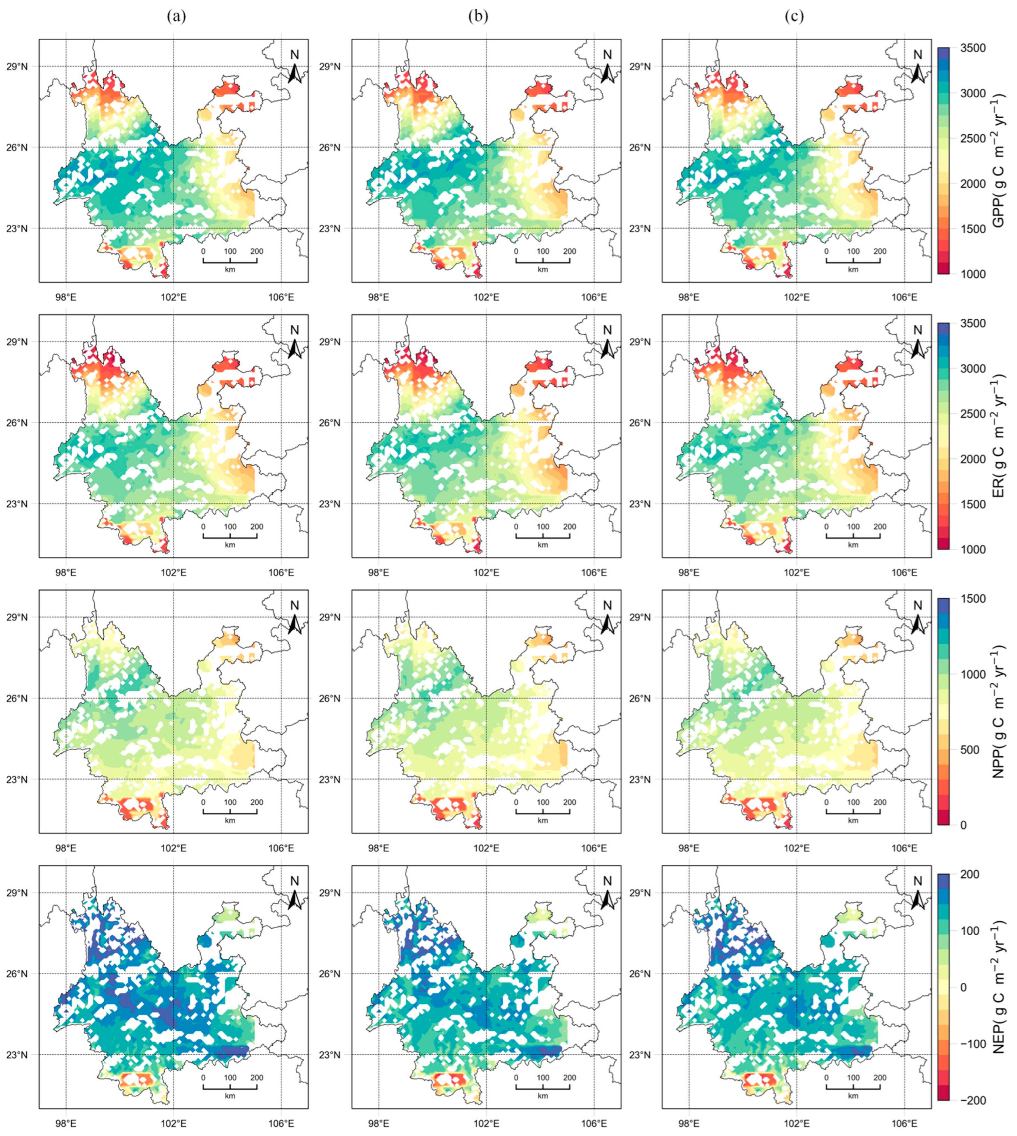
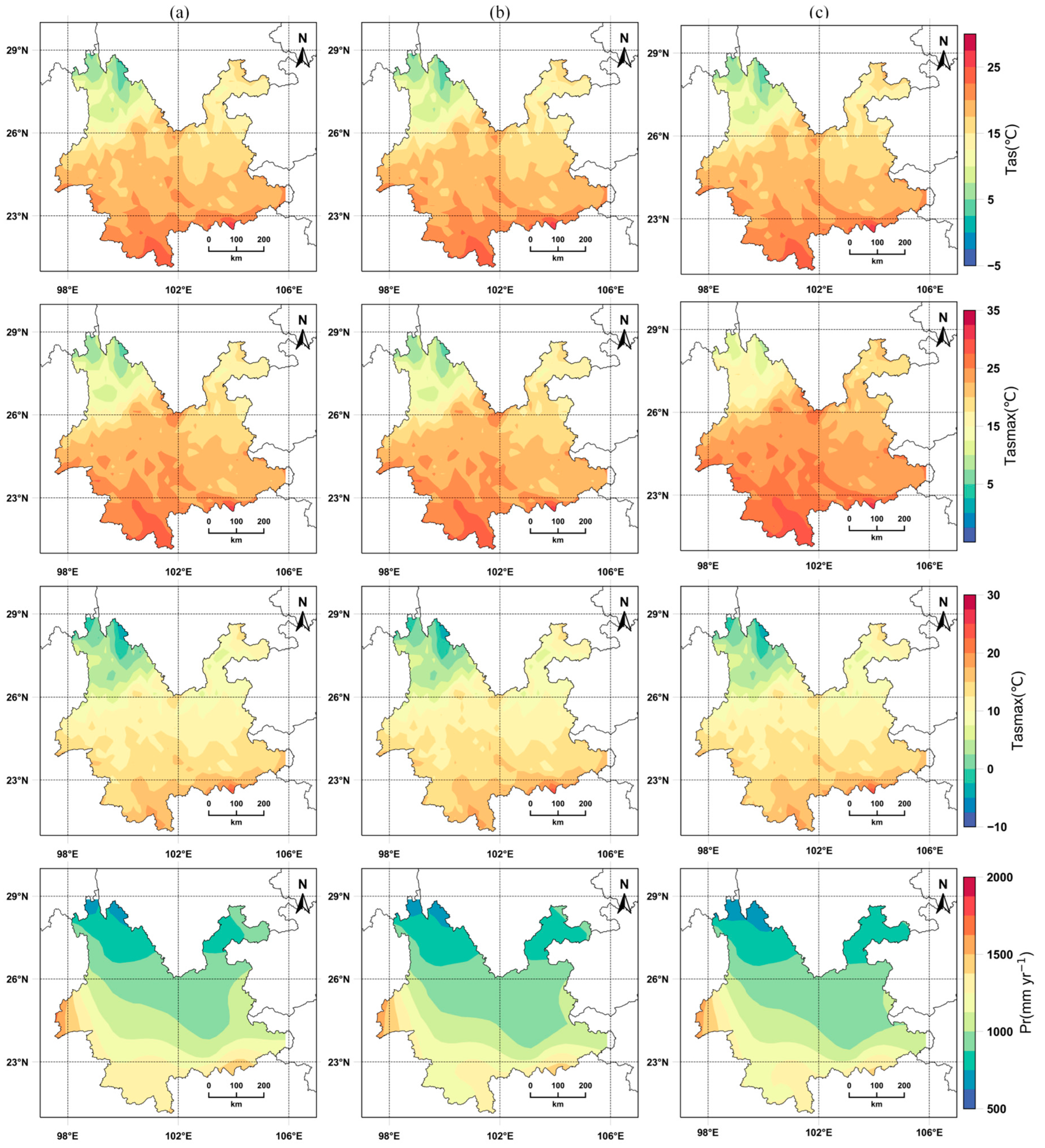
3.3. Spatiotemporal Pattern of Carbon Fluxes

The spatial analysis of forest ecosystem carbon fluxes in Yunnan Province revealed that the high value of GPP was located in the central and western part of Yunnan Province (98–102°E, 23–26°N), with annual mean values above 2500 gCm−2·yr−1, while in the northeast and east, GPP was relatively low, at less than 1500 gCm−2·yr−1. In the southern scattered areas under the SSP1-2.6 and SSP5-8.5 scenarios, there were low values of GPP (<1500 gCm−2·yr−1). The spatial distributions of ER and GPP were consistent, with ER > 2000 gCm−2·yr−1 in central and western Yunnan and ER between 1000 and 1800 gCm−2·yr−1 in the north and east. High NPP values of were located in the northwest, with annual mean values > 1000 gCm−2·yr−1 and above, while other regions had annual mean values below 900 gCm−2·yr−1, and the lowest values occurred in the south and east. The spatial component of NEP was significantly different from the other flux distributions, with high values located mainly in the western high-altitude region and in the central and southeastern regions. Areas with NEP greater than 100 gCm−2·yr−1 were higher than SSP5-8.5 in the SSP1-2.6 scenario and SSP2-4.5 scenario (Figure 6). The main reason was that the low temperature at high altitude suppresses forest respiration and thus increases the rate of carbon sequestration; in the forests of the southern region, photosynthesis leads to high forest productivity, but at the same time the respiration rate was also greater, and thus the rate of carbon sequestration was lower.

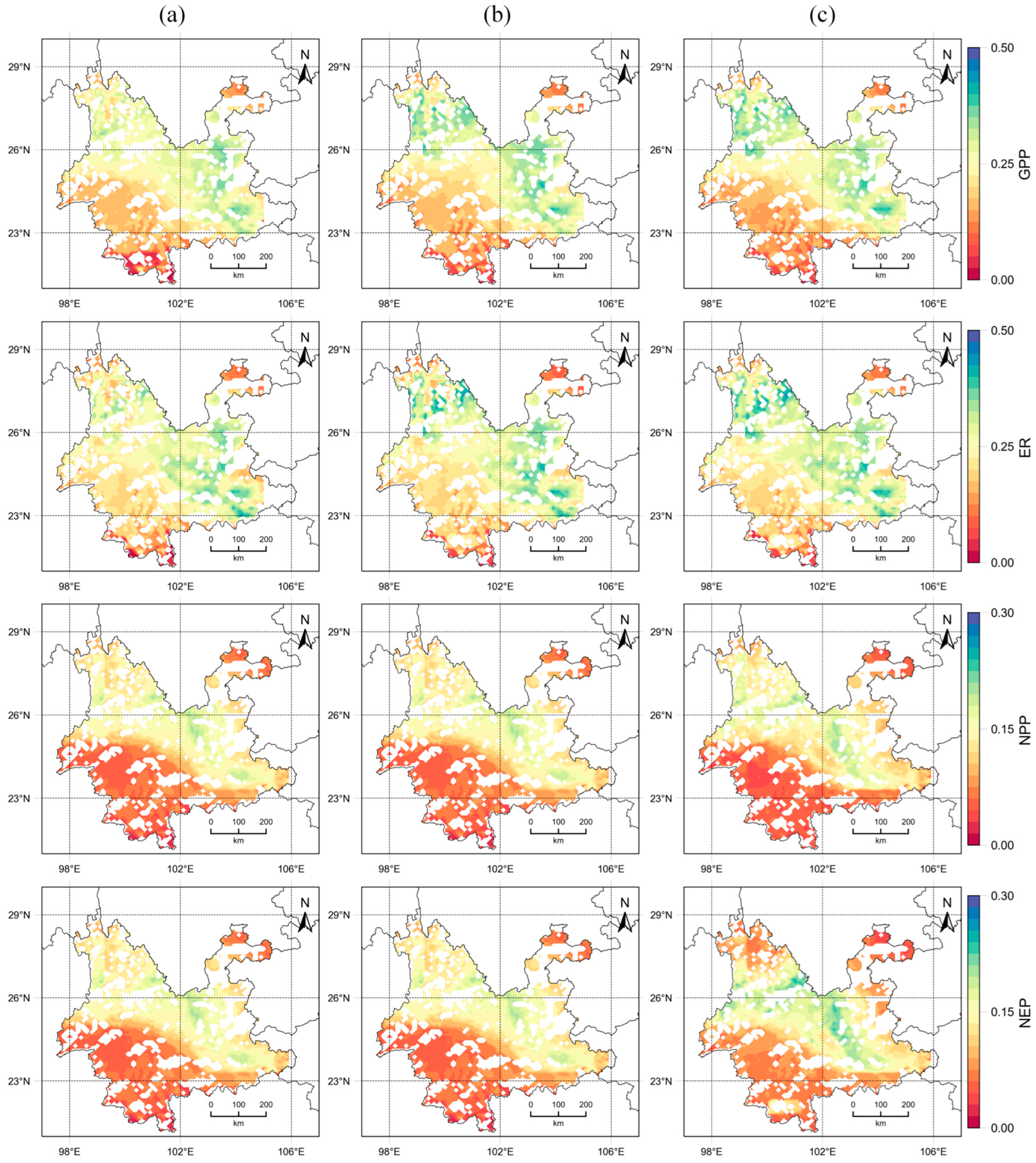
3.4. Coefficient of Variation of Carbon Fluxes

The analysis of carbon fluxes of forest ecosystems in Yunnan Province showed that the coefficient of variation (CV) displayed a decreasing pattern from southwest to northeast (Figure 7). The CV of GPP fluctuated between 0 and 0.5, with the smallest CV (<0.1) in the forest ecosystems of the Xishuangbanna region and the largest interannual variability (>0.3) in the Qujing and Wenshan regions of eastern Yunnan. The CV of 0–0.1 accounted for 3.04% of the total area, that of 0.1–0.3 accounted for 84.76% of the total area, and 12.20% of the area had a CV larger than 0.3. Under the SSP2-4.5 and SSP5-8.5 scenarios, the interannual variation of 0.1–0.3 accounted for approximately 70%, and the area larger than 0.3 accounted for 23.69% and 23.03%, respectively.
We discovered that the effects of different emission scenarios on ER were similar to those on the GPP pattern. The CV of ER was smaller in the south and northeast and higher in the northwest and southeast. The CV of ER in the SSP1-2.6 scenario was narrower than that in the other two scenarios, while the area with a CV greater than 0.3 was 16.13%, which was smaller than the values of 22.26% and 24.72% in the SSP2-4.5 and SSP5-8.5 scenarios, respectively. The area with a CV of 0.1–0.3 was 81.24%, which was higher than the values of 75.31% and 72.79% in the SSP2-4.5 and SSP5-8.5 scenarios, respectively.
The spatial variation in the CV of NPP under different climate change scenarios was not substantial, with 41.91%, 40.21%, and 41.36% in the regions with CVs below 0.1 under the SSP1-2.6, SSP2-4.5, and SSP5-8.5 scenarios, respectively. The CV was less than 0.05 in the Pu’er and Xishuangbanna regions in the central parts, while those in the Kunming and Yuxi regions were greater than 0.2.
The CV of NEP in the SSP1-2.6 and SSP5-8.5 scenarios were less than that in the SSP2-4.5 scenarios. The percentage of area with a CV less than 0.1 in the SSP1-2.6 and SSP5-8.5 scenarios was 51.76 and 51.07%, respectively, which was higher than that of SSP2-4.5 (42.91%). The percentage of area with a CV greater than 0.1 in the SSP1-2.6 and SSP5-8.5 scenarios was 48.24 and 48.93%, respectively, which was lower than the values of 56.03% for SSP2-4.5. The lower variability of forest carbon sequestration in the south than in the northwest and east is due to the lower interannual variability of temperature and precipitation in the south than in the north due to latitude and topography.

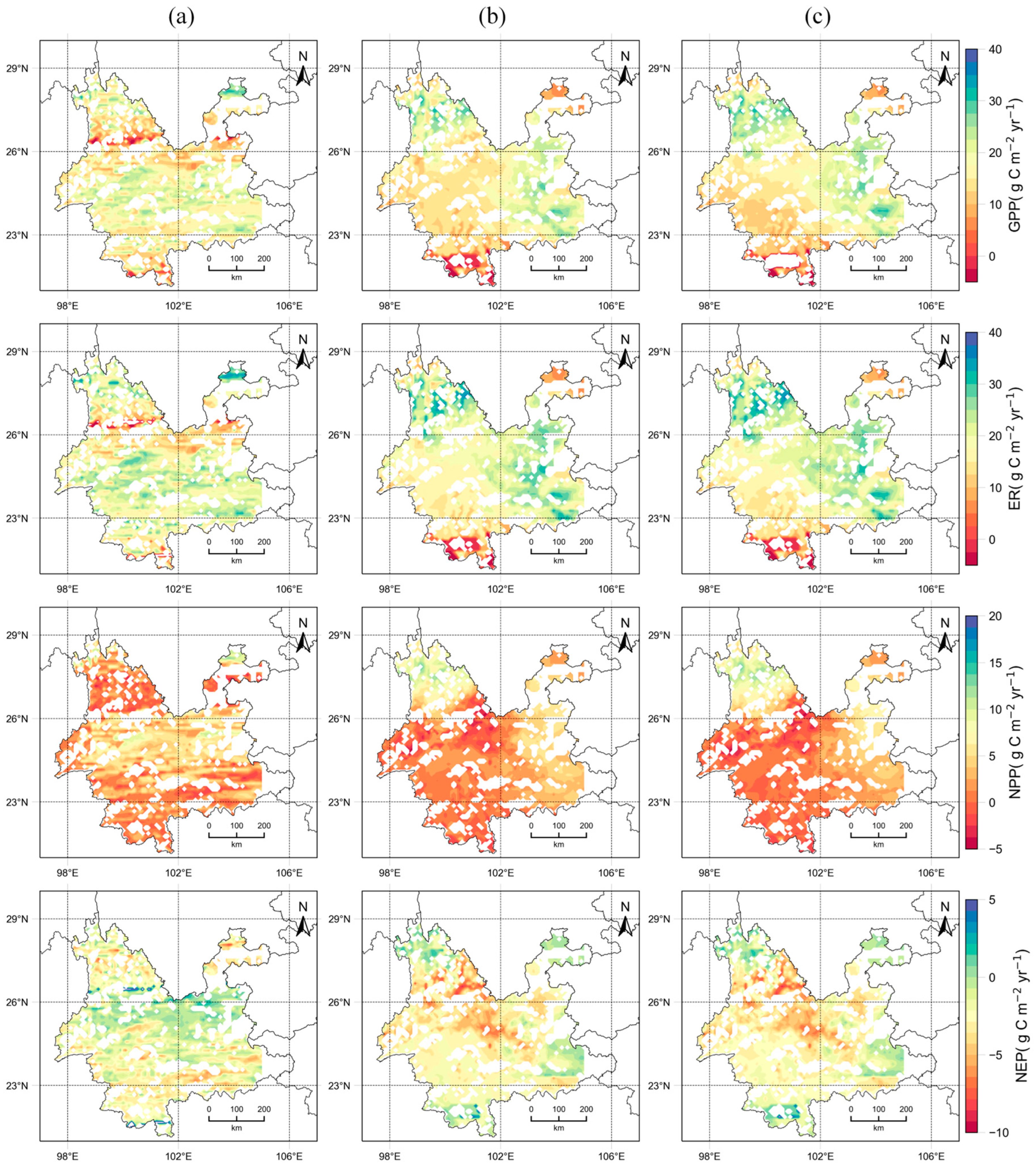
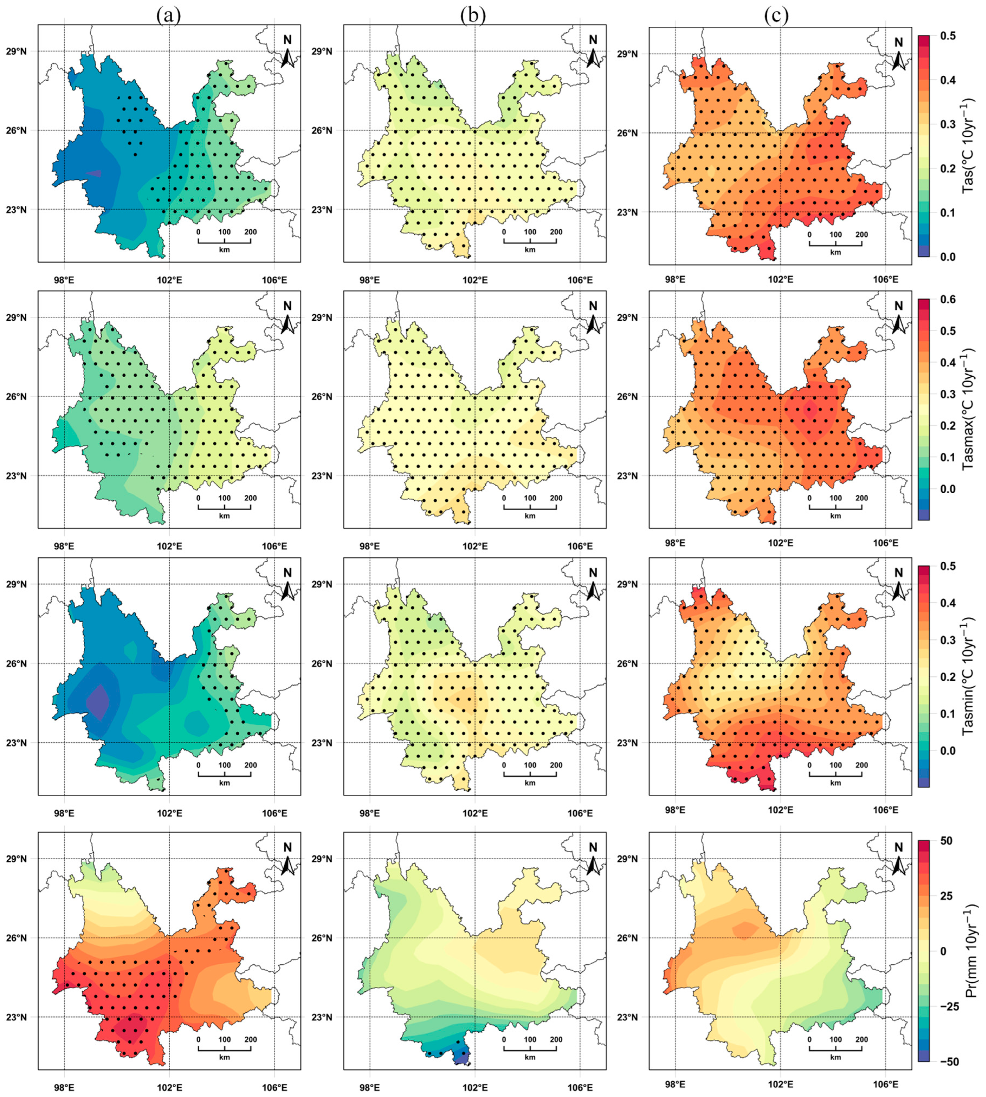
3.5. Trend of Carbon Fluxes

The analysis of GPP trends in Yunnan forest ecosystems revealed that the SSP1-2.6 scenario showed an increasing trend, accounting for 97.50% of the area, with a decreasing trend in GPP in the northwestern sporadic area (Figure 8). Under the SSP2-4.5 and SSP5-8.5 scenarios, the Xishuangbanna forests showed a decreasing trend, while in the northwestern and eastern regions, the forests showed an increasing trend (>25 gCm−2·yr−1). Additionally, 28.24% and 29.05% of the area with an increasing trend of >20 gCm−2·yr−1 under the SSP1-2.6 and SSP5-8.5 scenarios were higher than the value of 22.14% under the SSP2-4.5 scenario.
The analysis of forest ecosystem ER trends in Yunnan revealed that the ER of forest ecosystems in the three scenarios showed an increasing trend in an area of >95%, but there were differences in the spatial distribution. The SSP1-2.6 scenario showed an increasing trend in Baoshan and Puer in the central and southern parts of the country and a slight decrease in the northwestern part. The SSP2-4.5 and SSP5-8.5 scenarios showed a decreasing trend in the ER of the Xishuangbanna forest in the southern part of the country and an increasing trend in the ER of the Yuxi forest in the eastern part of Diqing in the northwestern part (>20 gCm−2·yr−1).
The proportion of area with a decreasing NPP trend under the three scenarios was 15–20%, with the largest proportion of area decreasing under SSP5-8.5 (up to 19.13%). The largest proportions of area with an increasing NPP trend between 0 and 5 gCm−2·yr−1 were 53.51, 60.30, and 52.96% for SSP1-2.6, SSP2-4.5, and SSP5-8.5, respectively. Under SSP1-2.6, NPP showed a decreasing trend mainly in Diqing and Nujiang, and SSP2-4.5 and SSP5-8.5 mainly had decreasing NPP trends in Chuxiong and Kunming.
Over the next 40 years, the NEP of more than 85% of forest ecosystems will decrease, with that in SSP2-4.5 and SSP5-8.5 decreasing mainly in Lijiang and Dali in the north with a downward trend of −5 gCm−2·yr−1 and that in SSP1-2.6 decreasing mainly in Wenshan in the south. Because the rising rate of ER in this region was higher than the rising rate of GPP, NEP showed a downward trend. The forests with an increasing NEP trend under the three scenarios were mainly located in the northwestern and eastern regions.

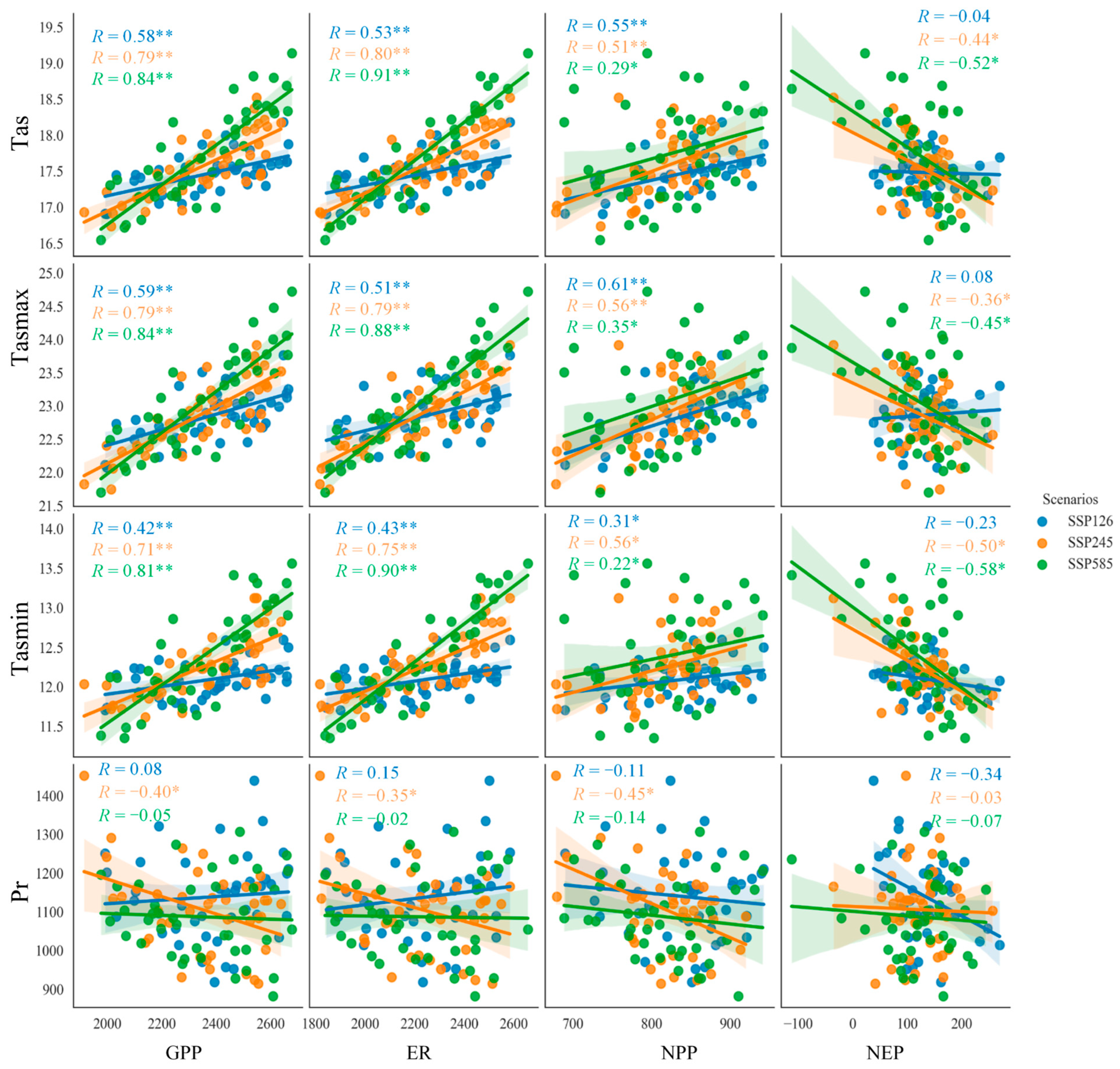
3.6. Driving Meteorological Factors of Carbon Fluxes

This study detected that temperature strongly affected the GPP and ER of forest ecosystems through correlation analysis. The mean temperature correlations with GPP were 0.59, 0.79, and 0.84 (p < 0.01), and those with ER were 0.53, 0.80, and 0.91 for the SSP1-2.6, SSP2-4.5, and SSP5-8.5 scenarios (p < 0.01), respectively (Figure 9). This result indicates that the positive correlations between temperature and GPP and ER were more significant in the high-emission scenarios. It was noteworthy that the negative correlation between NPP and NEP and temperature became increasingly obvious in the SSP2-4.5 and SSP5-8.5 scenarios, and the correlation coefficient between temperature and NEP was −0.04 (SSP1-2.6) shifted to −0.52 (SSP5-8.5). Under the SSP2-4.5 scenario, precipitation was significantly negatively correlated with GPP, ER, and NPP (p < 0.05), but there was no significant correlation between precipitation and carbon flux under the SSP1-2.6 and SSP5-8.5 scenarios. Correlation coefficients between NEP and precipitation were −0.34, −0.03, and −0.07 in SSP1-2.6, SSP2-4.5, and SSP5-8.5 (p > 0.05), respectively.
The contribution of different meteorological factors to carbon fluxes was quantified using linear regression. The mean temperature contributed 399.30, 364.97, and 257.42 gC·m−2·yr−1 to the increase in GPP for SSP1-2.6, SSP2-4.5, and SSP5-8.5, respectively (Table 4). Similarly, mean temperature contributed 406.69, 396.08, and 310.76 g·C·m−2·yr−1 to the increase in ER for SSP1-2.6, SSP2-4.5, and SSP5-8.5, respectively. Likewise, average temperature contributed 122.26, 64.39, and 29.26 gC·m−2·yr−1 to the increase in NPP for SSP1-2.6, SSP2-4.5, and SSP5-8.5, respectively. The contribution of temperature to NEP varied among future climate change scenarios, and the correlation between temperature and NEP was not significant in the SSP1-2.6 scenario, but the average temperature contributions to NEP were −49.11 and −53.34 gC·m−2·yr−1 in the SSP2-4.5 and SSP5-8.5 scenarios, respectively. Precipitation was significantly negatively correlated with ER, GPP, and NPP, with contributions of 0.71, 0.69, and 0.23 gC·m−2·yr−1, respectively.

4. Discussion

4.1. Spatiotemporal Distribution and Variability of Carbon Fluxes

Carbon fluxes in forest ecosystems tend to exhibit high spatial variability due to interactions between factors, such as climatic conditions, topography, and soil fertility [19,33,40]. We found that ER and GPP roughly showed a decreasing distribution from south to north and from west to east, while NPP and NEP showed a divergent pattern that was high in the northwest and central area and low in the south and east. The highest carbon sinks occurred in the northwestern alpine forest zone, and the lowest occur in tropical rainforest ecosystems. This was consistent with the spatial distribution of forest ecosystem observations in Yunnan [73].
This study found that forest ecosystems in Yunnan peaked in the 2030s and will generally show a declining trend after 2035. This was generally consistent with the assessments of other models [74,75,76]. This similarity suggests that effective management measures for existing forests are needed to maintain a high rate of carbon uptake after 2035 [76]. The reason for this was mainly that the increase in temperature and decrease in precipitation may lead to the occurrence of future structural droughts, which will have a significant negative impact on forests that may be converted from carbon sinks to carbon sources.
Different climate change scenarios have important impacts on the carbon sequestration potential of forest ecosystems. This study revealed that the carbon sequestration rate of forest ecosystems in Yunnan under the SSP1-2.6 scenario was higher than that under SSP2-4.5 and SSP5-8.5, which was mainly caused by the spatial heterogeneity of meteorological factors. Our analysis of the spatial distribution and trends of future meteorological data showed that the temperature increase in Yunnan under the SSP1-2.6 scenario was smaller than that under the other scenarios, and precipitation was significantly greater in the southwest.
The smaller CV of forest in the southwest was mainly due to the lower altitude and lower variability of temperature and precipitation than that in the northwest and northern regions (Figure 1a and Figure 8).

4.2. Driving Meteorological Factors of Carbon Fluxes

The analysis of the spatial distribution and significance of future climate factors for different climate change scenarios in Yunnan revealed a decreasing pattern of Tas, Tasmax, and Tasmin from southeast to northwest, which was consistent with historical climate change. The precipitation distribution pattern was mainly decreasing from southwest to northeast (Figure 10).
In both SSP5-8.5 and SSP2-4.5 scenarios, Tas, Tasmax, and Tasmin increased significantly in the study area. However, the temperature increase in the SSP2-4.5 scenario was smaller than that in the SSP5-8.5. In the SSP1-2.6 scenario, Tas, Tasmax, and Tasmin passed the significance test in the eastern and northern parts of Yunnan (p < 0.05). Precipitation increased significantly from southwest to northeast in the SSP1-2.6 scenario (>20 mm 10 yr−1), but the trend of precipitation change was not significant in the SSP2-4.5 and SSP5-8.5 scenarios (Figure 11).
The interannual variability of climate factors under different climate change scenarios was characterized by phases (Figure 12). The differences of Tas, Tasmax, and Tasmin for the three climate change scenarios were not significant in 2020–2040, while the Tas, Tasmax, and Tasmin under the SSP5-8.5 scenario in 2040–2060 were significantly higher than those under SSP1-2.6 and SSP2-4.5. The interannual variability of precipitation was not significant under the three climate change scenarios, but precipitation was higher under the SSP126 scenario than under SSP245 and SSP585 after 2040.
We compared the changes in climate factors for 2020–2060 under different climate change scenarios relative to the baseline period (2000–2019) [77] (Table 5). We found that the temperature increase from 2041–2060 was significantly higher than that from SSP2-4.5 and SSP1-2.6 under the SSP5-8.5 scenario, while the percentage increase in precipitation from 2020–2060 was smaller than that from SSP1-2.6 and SSP2-4.5.
Correlation and regression analyses revealed that meteorological factors contribute differently to carbon fluxes under different future climate scenarios. Under the SSP2-4.5 and SSP5-8.5 scenarios, temperature increases were detrimental to the carbon sinks of forest ecosystems (Figure 9). Several studies provide support for our findings. For example, high temperatures and drought in southwest China in spring 2010 resulted in 4% and 5% decreases in ecosystem GPP and NPP, respectively [78]. The frequency of extreme droughts was expected to increase by approximately 3.8 times per year under SSP5-8.5, and the resulting reduction in GPP was expected to increase by approximately 2.9 times [79,80]. There is an optimal temperature for vegetation photosynthesis, and in the subtropics the optimal temperature for vegetation photosynthesis is very close to the temperature during the growing season, which means that future warming will be detrimental to vegetation growth in the region [81]. The temperature increase will promote autotrophic and heterotrophic respiration in the ecosystem [82]. Eventually, the difference between GPP and ER will decrease, leading to a decrease in forest carbon sequestration in the subtropics under the high emission scenario.
The correlation between precipitation and carbon flux was not significant, and the correlation coefficients between NEP and precipitation were −0.34, −0.03, and −0.07 in SSP1-2.6, SSP2-4.5, and SSP5-8.5, respectively (Figure 9), which was not consistent with the study of national NEP by Yu et al. [19], mainly due to the different scales of the study area. At the low latitudes of this study area, precipitation promoted soil respiration [83,84], which reduced NEP, and in addition increased precipitation and reduced solar radiation, which decreased forest productivity [85].

4.3. Nature-Based Solutions to Enhance Forest Carbon Sinks

The basic spatial pattern of major carbon sink functional areas is determined by the macroscopic landscape, geography, and climate type of China [19,86]. The core concept of enhanced carbon sinks by NbS is to respect the laws of nature and utilize ecological processes while combining socio-economic conditions to optimize the regional natural–economic–social ecosystem and achieve unified ecological and socio-economic benefits [87]. According to our results, the forest carbon sequestration rate reaches its peak around the 2030s, and it is recommended to carry out regionally differentiated forest management measures according to different climate change scenarios after the 2030s, such as focusing on forest areas in the central region with a decreasing trend of carbon sequestration under the SSP5-8.5 scenario, and carrying out afforestation, thinning, and forest nurturing measures to maintain a high carbon sequestration rate (Table 6).

4.4. Limitations and Uncertainty

We estimated the carbon sequestration potential of forest ecosystems in Yunnan Province using the individual tree-based model FORCCHN. The uncertainty of the results mainly consisted of two parts: the model and the driving data. On the one hand, it was found through validation that there was a certain underestimation of GPP and ER and a slight overestimation of NEP, mainly because the model underestimation of GPP was smaller than the model underestimation of ER, thus leading to a slight overestimation of NEP [29]. The model considers only the input of litter matter in the soil carbon pool model due to the lack of localized parameters [31,56] and does not consider the input of microbial action and other carbon sources. On the other hand, there was uncertainty in the assessment of climate change scenarios by the GCM [89], which may lead to uncertainty in the driving data. In addition, this study did not consider the area of new afforestation, mainly because existing studies show that existing forests account for more than 90% of total carbon sequestration and that there are uncertainties in the distribution of afforestation [76]. In the future, we will further improve the FORCCHN model, especially by incorporating soil microorganisms to reduce its uncertainty, because soil carbon pools are very large and have an important role in estimating forest carbon sequestration [90]. Considering the increasing frequency of extreme climate events, we will develop a plant response module to extreme drought in the model to improve the accuracy of the simulation. In addition, the limitations of GCM data will be reduced by averaging multiple model ensembles [91].

5. Conclusions

By evaluating the carbon balance of Yunnan forest ecosystems from the period 2020–2060 based on the individual tree-based model FORCCHN, we have come to the following conclusions: First, both the GPP and ER of forest ecosystems showed an increasing trend under different climate change scenarios, with NPP peaking in the 2050s. Second, forest ecosystems in southwest China were still a carbon sink, but NEP will peak and begin to decline around the 2030s. Third, the forest NEP under the SSP1-2.6 scenario was higher than that under SSP2-4.5 and SSP5-8.5 in 2025-2035 and 2043–2058, and its carbon sequestration potential under the SSP1-2.6 scenario had a smaller CV than that under the other climate change scenarios. Forest carbon sequestration rates in southern China showed a decreasing trend, and a slight increasing trend in central and northwestern China. Finally, GPP, NPP, and ER were significantly and positively correlated with temperature and insignificantly correlated with precipitation, and rising temperatures will have a negative and destabilizing effect on forest carbon sinks. The inhibitory effect on carbon sequestration increased significantly with increasing temperature.
Based on spatial and temporal carbon sequestration and the variability and trend characteristics of forests under different scenarios, we proposed that a series of management measures could be implemented to improve the carbon sequestration capacity of forests in southwest China. After the 2030s, forest management measures can be carried out for forests in the southern region under the SSP1-2.6 scenario, while forest governance is recommended for Dali and Chuxiong in the central region under the SSP2-4.5 and SSP5-8.5 scenarios. These measures included fire prevention, pest and disease prevention, nurturing young forests, thinning, fertilization, and management of dead wood to further enhance the forest’s ability to sequester CO2 from the atmosphere.

Supplementary Materials

The following supporting information can be downloaded at: https://www.mdpi.com/article/10.3390/rs15051442/s1, Table S1: Physiological and ecological parameters of the nine basic types of trees in the model.

Author Contributions

Conceptualization, X.Y. and F.L.; methodology, X.Y. and F.L.; software, F.L.; validation, F.L.; formal analysis, F.L.; data curation, F.L.; writing—original draft preparation, F.L.; writing—review and editing, F.L., Y.S. and X.Y.; visualization, F.L.; supervision, X.Y.; funding acquisition, X.Y. All authors have read and agreed to the published version of the manuscript.

Funding

This research was supported by the State Key Laboratory of Earth Surface Processes and Resource Ecology (2022-GS-01) and the National Key Research and Development Program of China (2019YFA0606904 & 2018YFC509003).

Data Availability Statement

CIMP6 products are from the website https://esgf-node.llnl.gov/projects/cmip6/, accessed on 2 July 2022; soil data are available at http://www.issas.ac.cn/, accessed on 6 June 2022; the ChinaFLUX dataset can be downloaded at http://www.chinaflux.org/, accessed on 16 May 2021; CO2 data are available at https://climate.nasa.gov/vital-signs/carbon-dioxide/, accessed on 10 October 2022; MODIS C6 LAI data are available at http://globalchange.bnu.edu.cn/research/laiv6, accessed on 2 October 2022).

Conflicts of Interest

The authors declare no conflict of interest.

References

  1. Liu, Z.; Deng, Z.; He, G.; Wang, H.; Zhang, X.; Lin, J.; Qi, Y.; Liang, X. Challenges and opportunities for carbon neutrality in China. Nat. Rev. Earth Environ. 2022, 3, 141–155. [Google Scholar] [CrossRef]
  2. Piao, S.; Yue, C.; Ding, J.; Guo, Z. Perspectives on the role of terrestrial ecosystems in the ‘carbon neutrality’ strategy. Sci. China Earth Sci. 2022, 65, 1178–1186. [Google Scholar] [CrossRef]
  3. Mallapaty, S. How China could be carbon neutral by mid-century. Nature 2020, 586, 482–483. [Google Scholar] [CrossRef]
  4. Dixon, R.K.; Solomon, A.M.; Brown, S.; Houghton, R.A.; Trexier, M.C.; Wisniewski, J. Carbon pools and flux of global forest ecosystems. Science 1994, 263, 185–190. [Google Scholar] [CrossRef]
  5. Fang, J.Y.; Chen, A.P.; Peng, C.H.; Zhao, S.Q.; Ci, L. Changes in forest biomass carbon storage in China between 1949 and 1998. Science 2001, 292, 2320–2322. [Google Scholar] [CrossRef]
  6. Pacala, S.W.; Hurtt, G.C.; Baker, D.; Peylin, P.; Houghton, R.A.; Birdsey, R.A.; Heath, L.; Sundquist, E.T.; Stallard, R.F.; Ciais, P.; et al. Consistent land- and atmosphere-based U.S. carbon sink estimates. Science 2001, 292, 2316–2320. [Google Scholar] [CrossRef] [Green Version]
  7. Fang, J.Y.; Yu, G.R.; Liu, L.L.; Hu, S.J.; Chapin, F.S. Climate change, human impacts, and carbon sequestration in China INTRODUCTION. Proc. Natl. Acad. Sci. USA 2018, 115, 4015–4020. [Google Scholar] [CrossRef] [Green Version]
  8. Tang, X.L.; Zhao, X.; Bai, Y.F.; Tang, Z.Y.; Wang, W.T.; Zhao, Y.C.; Wan, H.W.; Xie, Z.Q.; Shi, X.Z.; Wu, B.F.; et al. Carbon pools in China’s terrestrial ecosystems: New estimates based on an intensive field survey. Proc. Natl. Acad. Sci. USA 2018, 115, 4021–4026. [Google Scholar] [CrossRef] [Green Version]
  9. Liu, J.; Chen, J.M.; Cihlar, J.; Park, W.M. A process-based boreal ecosystem productivity simulator using remote sensing inputs. Remote Sens. Environ. 1997, 62, 158–175. [Google Scholar] [CrossRef]
  10. Sitch, S.; Smith, B.; Prentice, I.C.; Arneth, A.; Bondeau, A.; Cramer, W.; Kaplan, J.O.; Levis, S.; Lucht, W.; Sykes, M.T.; et al. Evaluation of ecosystem dynamics, plant geography and terrestrial carbon cycling in the LPJ dynamic global vegetation model. Global Chang. Biol. 2003, 9, 161–185. [Google Scholar] [CrossRef]
  11. Piao, S.; Ciais, P.; Lomas, M.; Beer, C.; Liu, H.; Fang, J.; Friedlingstein, P.; Huang, Y.; Muraoka, H.; Son, Y.; et al. Contribution of climate change and rising CO2 to terrestrial carbon balance in East Asia: A multi-model analysis. Glob. Planet Chang. 2011, 75, 133–142. [Google Scholar] [CrossRef]
  12. Parton, W.J.; Scurlock, J.M.O.; Ojima, D.S.; Gilmanov, T.G.; Scholes, R.J.; Schimel, D.S.; Kirchner, T.; Menaut, J.C.; Seastedt, T.; Moya, E.G.; et al. Observations and modeling of biomass and soil organic matter dynamics for the grassland biome worldwide. Glob. Biogeochem. Cycles 1993, 7, 785–809. [Google Scholar] [CrossRef] [Green Version]
  13. Gurney, K.R.; Law, R.M.; Denning, A.S.; Rayner, P.J.; Baker, D.; Bousquet, P.; Bruhwiler, L.; Chen, Y.H.; Ciais, P.; Fan, S.; et al. Towards robust regional estimates of CO2 sources and sinks using atmospheric transport models. Nature 2002, 415, 626–630. [Google Scholar] [CrossRef] [Green Version]
  14. Thompson, R.L.; Patra, P.K.; Chevallier, F.; Maksyutov, S.; Law, R.M.; Ziehn, T.; van der Laan-Luijkx, I.T.; Peters, W.; Ganshin, A.; Zhuravlev, R.; et al. Top-down assessment of the Asian carbon budget since the mid 1990s. Nat. Commun. 2016, 7, 10724. [Google Scholar] [CrossRef] [Green Version]
  15. Wang, J.; Feng, L.; Palmer, P.I.; Liu, Y.; Fang, S.X.; Bosch, H.; O’Dell, C.W.; Tang, X.P.; Yang, D.X.; Liu, L.X.; et al. Large Chinese land carbon sink estimated from atmospheric carbon dioxide data. Nature 2020, 586, 720–723. [Google Scholar] [CrossRef]
  16. Ciais, P.; Tan, J.; Wang, X.; Roedenbeck, C.; Chevallier, F.; Piao, S.L.; Moriarty, R.; Broquet, G.; Le Quere, C.; Canadell, J.G.; et al. Five decades of northern land carbon uptake revealed by the interhemispheric CO2 gradient. Nature 2019, 568, 221–225. [Google Scholar] [CrossRef] [Green Version]
  17. Ichii, K.; Ueyama, M.; Kondo, M.; Saigusa, N.; Kim, J.; Alberto, M.C.; Ardo, J.; Euskirchen, E.S.; Kang, M.; Hirano, T.; et al. New data-driven estimation of terrestrial CO2 fluxes in Asia using a standardized database of eddy covariance measurements, remote sensing data, and support vector regression. J. Geophys. Res. Biogeosci. 2017, 122, 767–795. [Google Scholar] [CrossRef]
  18. Fu, D.J.; Chen, B.Z.; Zhang, H.F.; Wang, J.; Black, T.A.; Amiro, B.D.; Bohrer, G.; Bolstad, P.; Coulter, R.; Rahman, A.F.; et al. Estimating landscape net ecosystem exchange at high spatial-temporal resolution based on Landsat data, an improved upscaling model framework, and eddy covariance flux measurements. Remote Sens. Environ. 2014, 141, 90–104. [Google Scholar] [CrossRef]
  19. Yu, G.R.; Chen, Z.; Piao, S.L.; Peng, C.H.; Ciais, P.; Wang, Q.F.; Li, X.R.; Zhu, X.J. High carbon dioxide uptake by subtropical forest ecosystems in the East Asian monsoon region. Proc. Natl. Acad. Sci. USA 2014, 111, 4910–4915. [Google Scholar] [CrossRef] [Green Version]
  20. Goulden, M.L.; Munger, J.W.; Fan, S.M.; Daube, B.C.; Wofsy, S.C. Exchange of carbon dioxide by a deciduous forest: Response to interannual climate variability. Science 1996, 271, 1576–1578. [Google Scholar] [CrossRef] [Green Version]
  21. Wofsy, S.C.; Goulden, M.L.; Munger, J.W.; Fan, S.M.; Bakwin, P.S.; Daube, B.C.; Bassow, S.L.; Bazzaz, F.A. Net Exchange of CO2 in a Mid-Latitude Forest. Science 1993, 260, 1314–1317. [Google Scholar] [CrossRef] [Green Version]
  22. Piao, S.L.; Ciais, P.; Friedlingstein, P.; Peylin, P.; Reichstein, M.; Luyssaert, S.; Margolis, H.; Fang, J.Y.; Barr, A.; Chen, A.P.; et al. Net carbon dioxide losses of northern ecosystems in response to autumn warming. Nature 2008, 451, 49–52. [Google Scholar] [CrossRef]
  23. Ciais, P.; Reichstein, M.; Viovy, N.; Granier, A.; Ogee, J.; Allard, V.; Aubinet, M.; Buchmann, N.; Bernhofer, C.; Carrara, A.; et al. Europe-wide reduction in primary productivity caused by the heat and drought in 2003. Nature 2005, 437, 529–533. [Google Scholar] [CrossRef]
  24. Sitch, S.; Huntingford, C.; Gedney, N.; Levy, P.E.; Lomas, M.; Piao, S.L.; Betts, R.; Ciais, P.; Cox, P.; Friedlingstein, P.; et al. Evaluation of the terrestrial carbon cycle, future plant geography and climate-carbon cycle feedbacks using five Dynamic Global Vegetation Models (DGVMs). Glob. Chang. Biol. 2008, 14, 2015–2039. [Google Scholar] [CrossRef]
  25. Peng, C.H.; Zhou, X.L.; Zhao, S.Q.; Wang, X.P.; Zhu, B.; Piao, S.L.; Fang, J.Y. Quantifying the response of forest carbon balance to future climate change in Northeastern China: Model validation and prediction. Glob. Planet Chang. 2009, 66, 179–194. [Google Scholar] [CrossRef]
  26. Friedlingstein, P.; O’Sullivan, M.; Jones, M.W.; Andrew, R.M.; Hauck, J.; Olsen, A.; Peters, G.P.; Peters, W.; Pongratz, J.; Sitch, S.; et al. Global Carbon Budget 2020. Earth Syst. Sci. Data 2020, 12, 3269–3340. [Google Scholar] [CrossRef]
  27. Piao, S.L.; He, Y.; Wang, X.H.; Chen, F.H. Estimation of China’s terrestrial ecosystem carbon sink: Methods, progress and prospects. Sci. China Earth Sci. 2022, 65, 641–651. [Google Scholar] [CrossRef]
  28. Zhao, J.F.; Yan, X.D.; Guo, J.P.; Jia, G.S. Evaluating Spatial-Temporal Dynamics of Net Primary Productivity of Different Forest Types in Northeastern China Based on Improved FORCCHN. PLoS ONE 2012, 7, e48131. [Google Scholar] [CrossRef]
  29. Ma, J.Y.; Shugart, H.H.; Yan, X.D.; Cao, C.G.; Wu, S.; Fang, J. Evaluating carbon fluxes of global forest ecosystems by using an individual tree-based model FORCCHN. Sci. Total Environ. 2017, 586, 939–951. [Google Scholar] [CrossRef]
  30. Fang, J.; Shugart, H.H.; Liu, F.; Yan, X.D.; Song, Y.K.; Lv, F.C. FORCCHN V2.0: An individual-based model for predicting multiscale forest carbon dynamics. Geosci. Model Dev. 2022, 15, 6863–6872. [Google Scholar] [CrossRef]
  31. Yan, X.; Zhao, J. Establishing and validating individual-based carbon budget model FORCCHN of forest ecosystems in China. Acta Ecol. Sin. 2007, 27, 2684–2694. [Google Scholar] [CrossRef]
  32. Rogelj, J.; Den Elzen, M.; Höhne, N.; Fransen, T.; Fekete, H.; Winkler, H.; Schaeffer, R.; Sha, F.; Riahi, K.; Meinshausen, M. Paris Agreement climate proposals need a boost to keep warming well below 2 C. Nature 2016, 534, 631–639. [Google Scholar] [CrossRef] [PubMed] [Green Version]
  33. Pan, Y.D.; Birdsey, R.A.; Fang, J.Y.; Houghton, R.; Kauppi, P.E.; Kurz, W.A.; Phillips, O.L.; Shvidenko, A.; Lewis, S.L.; Canadell, J.G.; et al. A Large and Persistent Carbon Sink in the World’s Forests. Science 2011, 333, 988–993. [Google Scholar] [CrossRef] [Green Version]
  34. Pugh, T.A.M.; Lindeskog, M.; Smith, B.; Poulter, B.; Arneth, A.; Haverd, V.; Calle, L. Role of forest regrowth in global carbon sink dynamics. Proc. Natl. Acad. Sci. USA 2019, 116, 4382–4387. [Google Scholar] [CrossRef] [Green Version]
  35. Zhu, X.J.; Yu, G.R.; He, H.L.; Wang, Q.F.; Chen, Z.; Gao, Y.N.; Zhang, Y.P.; Zhang, J.H.; Yan, J.H.; Wang, H.M.; et al. Geographical statistical assessments of carbon fluxes in terrestrial ecosystems of China: Results from upscaling network observations. Glob. Planet Chang. 2014, 118, 52–61. [Google Scholar] [CrossRef]
  36. Yao, Y.T.; Li, Z.J.; Wang, T.; Chen, A.P.; Wang, X.H.; Du, M.Y.; Jia, G.S.; Li, Y.N.; Li, H.Q.; Luo, W.J.; et al. A new estimation of China’s net ecosystem productivity based on eddy covariance measurements and a model tree ensemble approach. Agric. Forest Meteorol. 2018, 253, 84–93. [Google Scholar] [CrossRef]
  37. Tian, H.Q.; Melillo, J.; Lu, C.Q.; Kicklighter, D.; Liu, M.L.; Ren, W.; Xu, X.F.; Chen, G.S.; Zhang, C.; Pan, S.F.; et al. China’s terrestrial carbon balance: Contributions from multiple global change factors. Glob. Biogeochem. Cycles 2011, 25, Gb1007. [Google Scholar] [CrossRef] [Green Version]
  38. He, H.L.; Wang, S.Q.; Zhang, L.; Wang, J.B.; Ren, X.L.; Zhou, L.; Piao, S.L.; Yan, H.; Ju, W.M.; Gu, F.X.; et al. Altered trends in carbon uptake in China’s terrestrial ecosystems under the enhanced summer monsoon and warming hiatus. Natl. Sci. Rev. 2019, 6, 505–514. [Google Scholar] [CrossRef] [Green Version]
  39. Zhang, H.F.; Chen, B.Z.; van der Laan-Luijkx, I.T.; Chen, J.; Xu, G.; Yan, J.W.; Zhou, L.X.; Fukuyama, Y.; Tans, P.P.; Peters, W. Net terrestrial CO2 exchange over China during 2001–2010 estimated with an ensemble data assimilation system for atmospheric CO2. J. Geophys. Res. Atmos. 2014, 119, 3500–3515. [Google Scholar] [CrossRef] [Green Version]
  40. Piao, S.L.; Fang, J.Y.; Ciais, P.; Peylin, P.; Huang, Y.; Sitch, S.; Wang, T. The carbon balance of terrestrial ecosystems in China. Nature 2009, 458, 1009–1013. [Google Scholar] [CrossRef]
  41. Eyring, V.; Bony, S.; Meehl, G.A.; Senior, C.A.; Stevens, B.; Stouffer, R.J.; Taylor, K.E. Overview of the Coupled Model Intercomparison Project Phase 6 (CMIP6) experimental design and organization. Geosci. Model Dev. 2016, 9, 1937–1958. [Google Scholar] [CrossRef] [Green Version]
  42. O’Neill, B.C.; Tebaldi, C.; van Vuuren, D.P.; Eyring, V.; Friedlingstein, P.; Hurtt, G.; Knutti, R.; Kriegler, E.; Lamarque, J.F.; Lowe, J.; et al. The Scenario Model Intercomparison Project (ScenarioMIP) for CMIP6. Geosci. Model Dev. 2016, 9, 3461–3482. [Google Scholar] [CrossRef] [Green Version]
  43. You, Q.; Cai, Z.; Wu, F.; Jiang, Z.; Pepin, N.; Shen, S.S.P. Temperature dataset of CMIP6 models over China: Evaluation, trend and uncertainty. Clim. Dyn. 2021, 57, 17–35. [Google Scholar] [CrossRef]
  44. Wang, Y.; Zhou, B.; Qin, D.; Wu, J.; Gao, R.; Song, L. Changes in mean and extreme temperature and precipitation over the arid region of northwestern China: Observation and projection. Adv. Atmos. Sci. 2017, 34, 289–305. [Google Scholar] [CrossRef]
  45. Yang, Y.; Shi, Y.; Sun, W.; Chang, J.; Zhu, J.; Chen, L.; Wang, X.; Guo, Y.; Zhang, H.; Yu, L.; et al. Terrestrial carbon sinks in China and around the world and their contribution to carbon neutrality. Sci. China Life Sci. 2022, 65, 861–895. [Google Scholar] [CrossRef]
  46. Yu, L.; Gu, F.X.; Huang, M.; Tao, B.; Hao, M.; Wang, Z.S. Impacts of 1.5 degrees C and 2 degrees C Global Warming on Net Primary Productivity and Carbon Balance in China’s Terrestrial Ecosystems. Sustainability 2020, 12, 2849. [Google Scholar] [CrossRef] [Green Version]
  47. Ji, J.J.; Huang, M.; Li, K.R. Prediction of carbon exchanges between China terrestrial ecosystem and atmosphere in 21st century. Sci. China Ser. D 2008, 51, 885–898. [Google Scholar] [CrossRef]
  48. Han, P.; Zeng, N.; Zhang, W.; Cai, Q.; Yang, R.; Yao, B.; Lin, X.; Wang, G.; Liu, D.; Yu, Y. Decreasing emissions and increasing sink capacity to support China in achieving carbon neutrality before 2060. arXiv 2021, arXiv:2102.10871. [Google Scholar]
  49. Li, Y.; Xu, X.; Wu, Z.; Fan, H.; Tong, X.; Liu, J. A forest type-specific threshold method for improving forest disturbance and agent attribution mapping. GIScience Remote Sens. 2022, 59, 1624–1642. [Google Scholar] [CrossRef]
  50. Zhu, D.; Yang, Q.; Xiong, K.; Xiao, H. Spatiotemporal Variations in Daytime and Night-Time Precipitation on the Yunnan–Guizhou Plateau from 1960 to 2017. Atmosphere 2022, 13, 415. [Google Scholar] [CrossRef]
  51. Jiang, W.; Yuan, P.; Chen, H.; Cai, J.; Li, Z.; Chao, N.; Sneeuw, N. Annual variations of monsoon and drought detected by GPS: A case study in Yunnan, China. Sci. Rep. 2017, 7, 5874. [Google Scholar] [CrossRef] [Green Version]
  52. Jiang, Z.; Hsu, Y.-J.; Yuan, L.; Huang, D. Monitoring time-varying terrestrial water storage changes using daily GNSS measurements in Yunnan, southwest China. Remote Sens. Environ. 2021, 254, 112249. [Google Scholar] [CrossRef]
  53. Yang, J.; Huang, X. The 30 m annual land cover dataset and its dynamics in China from 1990 to 2019. Earth Syst. Sci. Data 2021, 13, 3907–3925. [Google Scholar] [CrossRef]
  54. Zhu, Z.; Deng, X.; Zhao, F.; Li, S.; Wang, L. How Environmental Factors Affect Forest Fire Occurrence in Yunnan Forest Region. Forests 2022, 13, 1392. [Google Scholar] [CrossRef]
  55. Zhao, J.F.; Yan, X.D.; Jia, G.S. Simulating net carbon budget of forest ecosystems and its response to climate change in northeastern China using improved FORCCHN. Chin. Geogr. Sci. 2012, 22, 29–41. [Google Scholar] [CrossRef]
  56. Kirschbaum, M.U.F.; Paul, K.I. Modelling C and N dynamics in forest soils with a modified version of the CENTURY model. Soil Biol. Biochem. 2002, 34, 341–354. [Google Scholar] [CrossRef]
  57. Fang, J.; Lutz, J.A.; Shugart, H.H.; Liu, F.; Yan, X. Predicting soil mineralized nitrogen dynamics with fine root growth and microbial processes in temperate forests. Biogeochemistry 2022, 158, 21–37. [Google Scholar] [CrossRef]
  58. Jiang, H.; Apps, M.J.; Peng, C.; Zhang, Y.; Liu, J. Modelling the influence of harvesting on Chinese boreal forest carbon dynamics. For. Ecol. Manag. 2002, 169, 65–82. [Google Scholar] [CrossRef]
  59. Feng, X.; Fu, B.; Lu, N.; Zeng, Y.; Wu, B. How ecological restoration alters ecosystem services: An analysis of carbon sequestration in China’s Loess Plateau. Sci. Rep. 2013, 3, 1–5. [Google Scholar] [CrossRef] [Green Version]
  60. Fang, D.-M.; Zhou, G.-S.; Jiang, Y.-L.; Jia, B.-R.; Xu, Z.-Z.; Sui, X.-H. Impact of fire on carbon dynamics of Larix gmelinii forest in Daxing’an Mountains of North-East China: A simulation with CENTURY model. Ying Yong Sheng Tai Xue Bao J. Appl. Ecol. 2012, 23, 2411–2421. [Google Scholar]
  61. Crisp, D.; Pollock, H.R.; Rosenberg, R.; Chapsky, L.; Lee, R.A.M.; Oyafuso, F.A.; Frankenberg, C.; O’Dell, C.W.; Bruegge, C.J.; Doran, G.B.; et al. The on-orbit performance of the Orbiting Carbon Observatory-2 (OCO-2) instrument and its radiometrically calibrated products. Atmos. Meas. Tech. 2017, 10, 59–81. [Google Scholar] [CrossRef] [Green Version]
  62. Eldering, A.; O’Dell, C.W.; Wennberg, P.O.; Crisp, D.; Gunson, M.R.; Viatte, C.; Avis, C.; Braverman, A.; Castano, R.; Chang, A.; et al. The Orbiting Carbon Observatory-2: First 18 months of science data products. Atmos. Meas. Tech. 2017, 10, 549–563. [Google Scholar] [CrossRef] [Green Version]
  63. Ruimy, A.; Dedieu, G.; Saugier, B.J.G.B.C. TURC: A diagnostic model of continental gross primary productivity and net primary productivity. Glob. Biogeochem. Cycles 1996, 10, 269–285. [Google Scholar] [CrossRef]
  64. Niu, Z.; He, H.; Peng, S.; Ren, X.; Zhang, L.; Gu, F.; Zhu, G.; Peng, C.; Li, P.; Wang, J.; et al. A Process-Based Model Integrating Remote Sensing Data for Evaluating Ecosystem Services. J. Adv. Model. Earth Syst. 2021, 13, e2020MS002451. [Google Scholar] [CrossRef]
  65. Rambal, S.; Joffre, R.; Ourcival, J.M.; Cavender-Bares, J.; Rocheteau, A. The growth respiration component in eddy CO2 flux from a Quercus ilex mediterranean forest. Glob. Chang. Biol. 2004, 10, 1460–1469. [Google Scholar] [CrossRef]
  66. Krasting, J.P.; John, J.G.; Blanton, C.; McHugh, C.; Nikonov, S.; Radhakrishnan, A.; Rand, K.; Zadeh, N.T.; Balaji, V.; Durachta, J.; et al. NOAA-GFDL GFDL-ESM4 model output prepared for CMIP6 CMIP. Earth Syst. Grid Fed. 2018. [Google Scholar] [CrossRef]
  67. Wood, A.W.; Maurer, E.P.; Kumar, A.; Lettenmaier, D.P. Long-range experimental hydrologic forecasting for the eastern United States. J. Geophys. Res. Atmos. 2002, 107, ACL 6-1–ACL 6-15. [Google Scholar] [CrossRef]
  68. Shi, X.Z.; Yu, D.S.; Warner, E.D.; Pan, X.Z.; Petersen, G.W.; Gong, Z.G.; Weindorf, D.C. Soil Database of 1:1,000,000 Digital Soil Survey and Reference System of the Chinese Genetic Soil Classification System. Soil Surv. Horiz. 2004, 45, 129–136. [Google Scholar] [CrossRef]
  69. Li, H.; Wu, Y.; Liu, S.; Xiao, J. Regional contributions to interannual variability of net primary production and climatic attributions. Agric. For. Meteorol. 2021, 303, 108384. [Google Scholar] [CrossRef]
  70. Peng, S.; Chen, A.; Xu, L.; Cao, C.; Fang, J.; Myneni, R.B.; Pinzon, J.E.; Tucker, C.J.; Piao, S. Recent change of vegetation growth trend in China. Environ. Res. Lett. 2011, 6, 044027. [Google Scholar] [CrossRef]
  71. Wan, J.-Z.; Wang, C.-J.; Qu, H.; Liu, R.; Zhang, Z.-X. Vulnerability of forest vegetation to anthropogenic climate change in China. Sci. Total Environ. 2018, 621, 1633–1641. [Google Scholar] [CrossRef]
  72. Yuan, H.; Dai, Y.; Xiao, Z.; Ji, D.; Shangguan, W. Reprocessing the MODIS Leaf Area Index products for land surface and climate modelling. Remote Sens. Environ. 2011, 115, 1171–1187. [Google Scholar] [CrossRef]
  73. Fei, X.; Song, Q.; Zhang, Y.; Liu, Y.; Sha, L.; Yu, G.; Zhang, L.; Duan, C.; Deng, Y.; Wu, C.; et al. Carbon exchanges and their responses to temperature and precipitation in forest ecosystems in Yunnan, Southwest China. Sci. Total Environ. 2018, 616–617, 824–840. [Google Scholar] [CrossRef]
  74. Mao, F.; Du, H.; Zhou, G.; Zheng, J.; Li, X.; Xu, Y.; Huang, Z.; Yin, S. Simulated net ecosystem productivity of subtropical forests and its response to climate change in Zhejiang Province, China. Sci. Total Environ. 2022, 838, 155993. [Google Scholar] [CrossRef]
  75. Cai, W.; He, N.; Li, M.; Xu, L.; Wang, L.; Zhu, J.; Zeng, N.; Yan, P.; Si, G.; Zhang, X.; et al. Carbon sequestration of Chinese forests from 2010 to 2060: Spatiotemporal dynamics and its regulatory strategies. Sci. Bull. 2022, 67, 836–843. [Google Scholar] [CrossRef]
  76. He, N.; Wen, D.; Zhu, J.; Tang, X.; Xu, L.; Zhang, L.; Hu, H.; Huang, M.; Yu, G. Vegetation carbon sequestration in Chinese forests from 2010 to 2050. Glob. Chang. Biol. 2017, 23, 1575–1584. [Google Scholar] [CrossRef]
  77. Wu, J.; Gao, X.; Giorgi, F.; Chen, D. Changes of effective temperature and cold/hot days in late decades over China based on a high resolution gridded observation dataset. Int. J. Climatol. 2017, 37, 788–800. [Google Scholar] [CrossRef]
  78. Zhang, L.; Xiao, J.; Li, J.; Wang, K.; Lei, L.; Guo, H. The 2010 spring drought reduced primary productivity in southwestern China. Environ. Res. Lett. 2012, 7, 045706. [Google Scholar] [CrossRef] [Green Version]
  79. Xu, C.; McDowell, N.G.; Fisher, R.A.; Wei, L.; Sevanto, S.; Christoffersen, B.O.; Weng, E.; Middleton, R.S. Increasing impacts of extreme droughts on vegetation productivity under climate change. Nat. Clim. Chang. 2019, 9, 948–953. [Google Scholar] [CrossRef] [Green Version]
  80. Shi, H.; Tian, H.; Lange, S.; Yang, J.; Pan, S.; Fu, B.; Reyer, C.P.O. Terrestrial biodiversity threatened by increasing global aridity velocity under high-level warming. Proc. Natl. Acad. Sci. USA 2021, 118, e2015552118. [Google Scholar] [CrossRef]
  81. Xia, J.; Chen, J.; Piao, S.; Ciais, P.; Luo, Y.; Wan, S. Terrestrial carbon cycle affected by non-uniform climate warming. Nat. Geosci. 2014, 7, 173–180. [Google Scholar] [CrossRef]
  82. Yvon-Durocher, G.; Caffrey, J.M.; Cescatti, A.; Dossena, M.; Giorgio, P.D.; Gasol, J.M.; Montoya, J.M.; Pumpanen, J.; Staehr, P.A.; Trimmer, M. Reconciling the temperature dependence of respiration across timescales and ecosystem types. Nature 2012, 487, 472–476. [Google Scholar] [CrossRef]
  83. Thomas, A.D.; Hoon, S.R.; Dougill, A.J. Soil respiration at five sites along the Kalahari Transect: Effects of temperature, precipitation pulses and biological soil crust cover. Geoderma 2011, 167–168, 284–294. [Google Scholar] [CrossRef]
  84. Wang, Z.; McKenna, T.P.; Schellenberg, M.P.; Tang, S.; Zhang, Y.; Ta, N.; Na, R.; Wang, H. Soil respiration response to alterations in precipitation and nitrogen addition in a desert steppe in northern China. Sci. Total Environ. 2019, 688, 231–242. [Google Scholar] [CrossRef]
  85. Fyllas, N.M.; Bentley, L.P.; Shenkin, A.; Asner, G.P.; Atkin, O.K.; Díaz, S.; Enquist, B.J.; Farfan-Rios, W.; Gloor, E.; Guerrieri, R.; et al. Solar radiation and functional traits explain the decline of forest primary productivity along a tropical elevation gradient. Ecol. Lett. 2017, 20, 730–740. [Google Scholar] [CrossRef]
  86. Chen, Z.; Yu, G.; Ge, J.; Sun, X.; Hirano, T.; Saigusa, N.; Wang, Q.; Zhu, X.; Zhang, Y.; Zhang, J. Temperature and precipitation control of the spatial variation of terrestrial ecosystem carbon exchange in the Asian region. Agric. For. Meteorol. 2013, 182, 266–276. [Google Scholar] [CrossRef]
  87. Wang, F.; Harindintwali, J.D.; Yuan, Z.; Wang, M.; Wang, F.; Li, S.; Yin, Z.; Huang, L.; Fu, Y.; Li, L.; et al. Technologies and perspectives for achieving carbon neutrality. Innovation 2021, 2, 100180. [Google Scholar] [CrossRef]
  88. Yu, G.; Zhu, J.; Xu, L.; He, N. Technological approaches to enhance ecosystem carbon sink in China: Nature-based solutions. Bull. Chin. Acad. Sci. 2022, 37, 490–501. [Google Scholar]
  89. Deser, C.; Lehner, F.; Rodgers, K.B.; Ault, T.; Delworth, T.L.; DiNezio, P.N.; Fiore, A.; Frankignoul, C.; Fyfe, J.C.; Horton, D.E.; et al. Insights from Earth system model initial-condition large ensembles and future prospects. Nat. Clim. Chang. 2020, 10, 277–286. [Google Scholar] [CrossRef]
  90. Zhang, Y.; Ai, J.; Sun, Q.; Li, Z.; Hou, L.; Song, L.; Tang, G.; Li, L.; Shao, G. Soil organic carbon and total nitrogen stocks as affected by vegetation types and altitude across the mountainous regions in the Yunnan Province, south-western China. CATENA 2021, 196, 104872. [Google Scholar] [CrossRef]
  91. Huang, P.; Ying, J. A Multimodel Ensemble Pattern Regression Method to Correct the Tropical Pacific SST Change Patterns under Global Warming. J. Clim. 2015, 28, 4706–4723. [Google Scholar] [CrossRef]
Figure 1. Topographic (a) and vegetation types (b) of Yunnan Province.
Remotesensing 15 01442 g001
Figure 2. Main process and flow chart of the FORCCHN model.
Remotesensing 15 01442 g002
Figure 3. Performance of FORCCHN in simulating the ER, GPP, and NEP of Xishuang Banna forests at different time scales. (a) daily scale data; (b)monthly scale data; (c)annual scale data.
Remotesensing 15 01442 g003
Figure 4. Interannual variation in carbon fluxes in forest ecosystems from 2020 to 2060.
Remotesensing 15 01442 g004
Figure 5. Violin plot of carbon fluxes in forest ecosystems from 2020 to 2060. (The tops and bottoms of each ‘box’ are the 25th and 75th percentiles of the samples, respectively. The point in the middle of each box denotes the median value. The upper and lower whiskers are the 5th and 95th percentiles of the samples, respectively).
Remotesensing 15 01442 g005
Figure 6. Spatial distribution of annual mean carbon fluxes in Yunnan Province from 2020 to 2060 under different emission scenarios: (a) SSP1-2.6; (b) SSP2-4.5; and (c) SSP5-8.5.
Remotesensing 15 01442 g006
Figure 7. Spatial distribution of the carbon flux coefficient of variation in Yunnan Province from 2020 to 2060 under different emission scenarios: (a) SSP1-2.6; (b) SSP2-4.5; and (c) SSP5-8.5.
Remotesensing 15 01442 g007
Figure 8. Spatial distribution of carbon flux trends in Yunnan Province from 2020 to 2060 under different emission scenarios: (a) SSP1-2.6; (b) SSP2-4.5; and (c) SSP5-8.5.
Remotesensing 15 01442 g008
Figure 9. Correlation of carbon fluxes with meteorological factors. ** represents p < 0.01, * represents p < 0.05.
Remotesensing 15 01442 g009
Figure 10. Spatial distribution of meteorological factors under different scenarios: (a) SSP1-2.6; (b) SSP2-4.5; (c) SSP5-8.5.
Remotesensing 15 01442 g010
Figure 11. Trends of meteorological factors and their significance under different SSPs scenarios: (a) SSP1-2.6; (b) SSP2-4.5; (c) SSP5-8.5.
Remotesensing 15 01442 g011
Figure 12. Interannual variation in meteorological factors under different SSPs scenarios.
Remotesensing 15 01442 g012
Table 1. Main features of the FORCCHN model.
FeaturesDescription
Initial conditionsField water holding capacity, soil carbon pool, soil nitrogen pool, LAI data or stand per wood check information on patch area.
Margin variablesDaily maximum temperature, minimum temperature, mean temperature, precipitation, relative air humidity, total radiation, mean wind speed, average air pressure, atmospheric CO2 concentration.
Substance balance programsComplete balance of carbon, nitrogen, and water in the atmosphere–soil–forest system.
Time steps and programsDaily per wood carbon and nitrogen uptake, litter fluxes, and respiratory fluxes.
Daily soil carbon, nitrogen, and water inputs and outputs.
Daily forest carbon, nitrogen uptake, and litter fluxes on patches.
Yearly per wood carbon accumulation, flower and fruit litter fluxes, and tree diameter at breast height growth, tree height growth, and branch height growth calculation.
Daily per wood carbon, nitrogen budgetConsidering total photosynthesis, maintenance respiration, growth respiration, photosynthetic product partitioning, and apoptosis, the use of a photosynthetic product buffer bank scheme makes resistance to climate extremes enhanced.
Daily soil carbon, nitrogen budgetA modified CENTURY model suitable for forest soils is used, so that the decomposition and respiration components of forest soils can be provisionally considered as well-founded in the absence of validation information.
Yearly tree growthCalculation of annual photosynthetic product distribution, flower and fruit drop, and tree diameter at breast height, tree height, height under branches, and potential maximum leaf volume considering buffer banks.
Table 2. Parameters of soil decomposition rate in the FORCCHN model.
SymbolUnitCarbon PoolValue
S11/dAboveground metabolic litter pool0.080
S21/dAboveground structural litter pool0.021
S31/dBelowground metabolic litter pool0.100
S41/dBelowground structural litter pool0.027
S51/dFine woody litter pool0.010
S61/dCoarse woody litter pool0.002
S71/dBelowground coarse litter pool0.002
S81/dActive soil organic matter pool0.040
S91/dSlow soil organic matter pool0.001
S101/dInert soil organic matter pool3.5 × 10−5
Table 3. Description of the data used in this study.
Data TypeNameSpatial
Resolution
Temporal
Resolution
Time
Periods
Source
Meteorological dataThe maximum temperature (Tasmax), minimum temperature (Tasmin), mean temperature (Tas), precipitation, wind speed, relative humidity, shortwave radiation, and pressure0.1°Daily2020–2060GFDL–ESM4 product, CMIP6.
Vegetation dataForest types0.1°---2007Editorial Board of Vegetation Map of China, CAS.
Vegetation dataLAI0.01Yearly2019MODIS C6 LAI
Soil dataSoil sand content, soil meal content, soil clay content, soil bulk density, soil field water0.1°------Nanjing Institute of Soil Research, CAS
Table 4. Trends and significance levels of carbon fluxes and meteorological factors.
Tasmax (°C)Tas (°C)Tasmin (°C)Pr (mm)
SSP1-2.6GPPy = −4332.54 + 294.02x **y = −4589.87 + 399.30x **y = −1914.98 + 355.83x **y = 2233.66 +0.14x
ERy = −4229.69 + 283.67x ** y = −4852.93 + 406.69x **y = −2677.10 + 407.77x **y = 1921.450 +0.29x
NPPy = −1397.67 + 98.07x **y = −1292.52 + 122.26x **y = 194.14 + 85.85x **y = 914.286 + 0.06x
NEPy = −102.84 + 10.36xy = 263.07 − 7.39xy = 762.12 − 51.94xy = 312.215 + 0.16x
SSP2-4.5GPPy = −4306.76 + 290.88x **y = −3745.29 + 346.97x **y = −2033.09 + 357.81x **y = 3129.95 − 0.71x *
ERy = −5199.02 + 324.58x **y = −4729.06 + 396.08x **y = −2944.22 + 422.31x **y = 2993.77 − 0.69x *
NPPy = −540.60 + 59.37x **y = −312.96 + 64.389x **y = 127.29 + 56.40x **y = 1069.232 − 0.23x *
NEPy = 892.27 − 33.70x *y = 983.78 − 49.11x *y = 911.13 − 64.50x *y = 136.18 − 0.01x
SSP5-8.5GPPy = −2892.23 + 227.32x **y = −2211.89 + 257.42x **y = −997.61 + 270.36x **y = 451.02 − 0.09x
ERy = −3957.49 + 268.25x **y = −3278.69 + 310.76x **y = −1929.62 + 335.82x **y = 915.51 − 0.09x
NPPy = 120.92 + 30.24x *y = 299.88 + 29.26x *y = 521.22 + 24.00x *y = 2274.18 − 0.04x
NEPy = 1065.26 − 40.93x *y = 1066.80 − 53.34x *y = 932.01 − 65.47x *y = 176.84 − 0.05x
(** represents p < 0.01, * represents p < 0.05).
Table 5. Changes in precipitation (%) and temperature (°C) in the Yunnan under different climate change scenarios (compared to 2000–2019) in the near term (2020–2040), and in the medium term (2040–2060).
SSP1-2.6SSP2-4.5SSP5-8.5
Time PeriodsPrTasTasmaxTasminPrTasTasmaxTasminPrTasTasmaxTasmin
2020–204038.633.893.222.5440.563.853.102.5736.223.763.012.49
2041–206045.494.103.482.7135.034.333.652.9934.774.754.123.36
Table 6. Qualitative evaluation of the effect of anthropogenic management measures on carbon sequestration [88].
Management MeasuresCarbon Fixation RateTechnology MaturityEnvironmental AdaptabilityPublic Acceptability
Afforestation and Reforestation**********
Returning farmland to forest**********
Natural forest restoration************
Forest Nurture********
Thinning********
The more asterisks, the stronger the carbon fixation rate or the more suitability for the promotion of the management measures.
Disclaimer/Publisher’s Note: The statements, opinions and data contained in all publications are solely those of the individual author(s) and contributor(s) and not of MDPI and/or the editor(s). MDPI and/or the editor(s) disclaim responsibility for any injury to people or property resulting from any ideas, methods, instructions or products referred to in the content.

