Article

Mapping Fractional Vegetation Coverage across Wetland Classes of Sub-Arctic Peatlands Using Combined Partial Least Squares Regression and Multiple Endmember Spectral Unmixing

1
Earth and Environmental Sciences, Lehigh University, Bethlehem, PA 18015, USA
2
US Fish and Wildlife Service, Kenai National Wildlife Refuge, Soldotna, AK 99669, USA
*
Author to whom correspondence should be addressed.
These authors contributed equally to this work.
Remote Sens. 2023, 15(5), 1440; https://doi.org/10.3390/rs15051440
Submission received: 17 January 2023 / Revised: 26 February 2023 / Accepted: 2 March 2023 / Published: 4 March 2023
(This article belongs to the Special Issue Application of Remote Sensing for Monitoring of Peatlands)

Abstract

:
Vegetation communities play a key role in governing the atmospheric-terrestrial fluxes of water, carbon, nutrients, and energy. The expanse and heterogeneity of vegetation in sub-arctic peatland systems makes monitoring change at meaningful spatial resolutions and extents challenging. We use a field-collected spectral endmember reference library to unmix hyperspectral imagery and map vegetation coverage at the level of plant functional type (PFT), across three wetland sites in sub-arctic Alaska. This study explores the optimization and parametrization of multiple endmember spectral mixture analysis (MESMA) models to estimate coverage of PFTs across wetland classes. We use partial least squares regression (PLSR) to identify a parsimonious set of critical bands for unmixing and compare the reference and modeled coverage. Unmixing, using a full set of 110-bands and a smaller set of 4-bands, results in maps that effectively discriminate between PFTs, indicating a small investment in fieldwork results in maps mirroring the true ground cover. Both sets of spectral bands differentiate between PFTs, but the 4-band unmixing library results in more accurate predictive mapping with lower computational cost. Reducing the unmixing reference dataset by constraining the PFT endmembers to those identified in the field-site produces only a small advantage for mapping, suggesting extensive fieldwork may not be necessary for MESMA to have a high explanatory value in these remote environments.

1. Introduction

Earth systems modeling relies on accurate estimates of vegetation composition and distribution to characterize atmospheric-terrestrial fluxes of water, carbon, nutrients, and energy. Within a landscape type, species richness positively correlates with rates of microbial activity and decomposition [1,2]. The composition of plant types influences soil temperature and moisture, which in turn regulates microbial activity and governs carbon and nitrogen cycling, and thus the long-term balance of greenhouse gas emission and sequestration [3,4,5,6,7,8]. The most recent iteration of the Model for Interdisciplinary Research on Climate, Earth System version 2 for Long-term (MIROC-ES2L) simulations, incorporates a land based biogeochemical component that links the interactions of soil nitrogen-carbon and vegetation [9]). Knowing the vegetation distribution in vast peatlands and at a realistic spatial scale is thus key for modeling these stores and fluxes.
Spectra containing multiple vegetation types require a deconvolution approach that can determine the fractional abundance of each vegetation component [10]. Image analysis algorithms like random forest and maximum likelihood result in hard-edged binning of pixels where each pixel represents one class of material. More advanced spectral unmixing tools, such as spectral mixture analysis (SMA) analyzes sub-pixel fractions of component materials. SMA can distinguish between materials that are spectrally and functionally similar such as between multiple anthropogenic surfaces or multiple plant functional types (PFTs) [11]. This ability to distinguish between materials that are spectrally similar, makes SMA well suited to systems like peatlands that exhibit fine scale variability in vegetation coverage [12].
Spectral unmixing compares each image pixel’s spectral profile to a spectral endmember reference set in order to identify the fraction of each endmember’s presence in the pixel. Simple unmixing models use a single set of endmembers to unmix each image [13], neglecting endmember variability [10,14,15]. MESMA is an extension of the simple unmixing model, in which number and types of endmembers are allowed to vary on a per pixel basis, thus accounting for endmember variability [16,17].
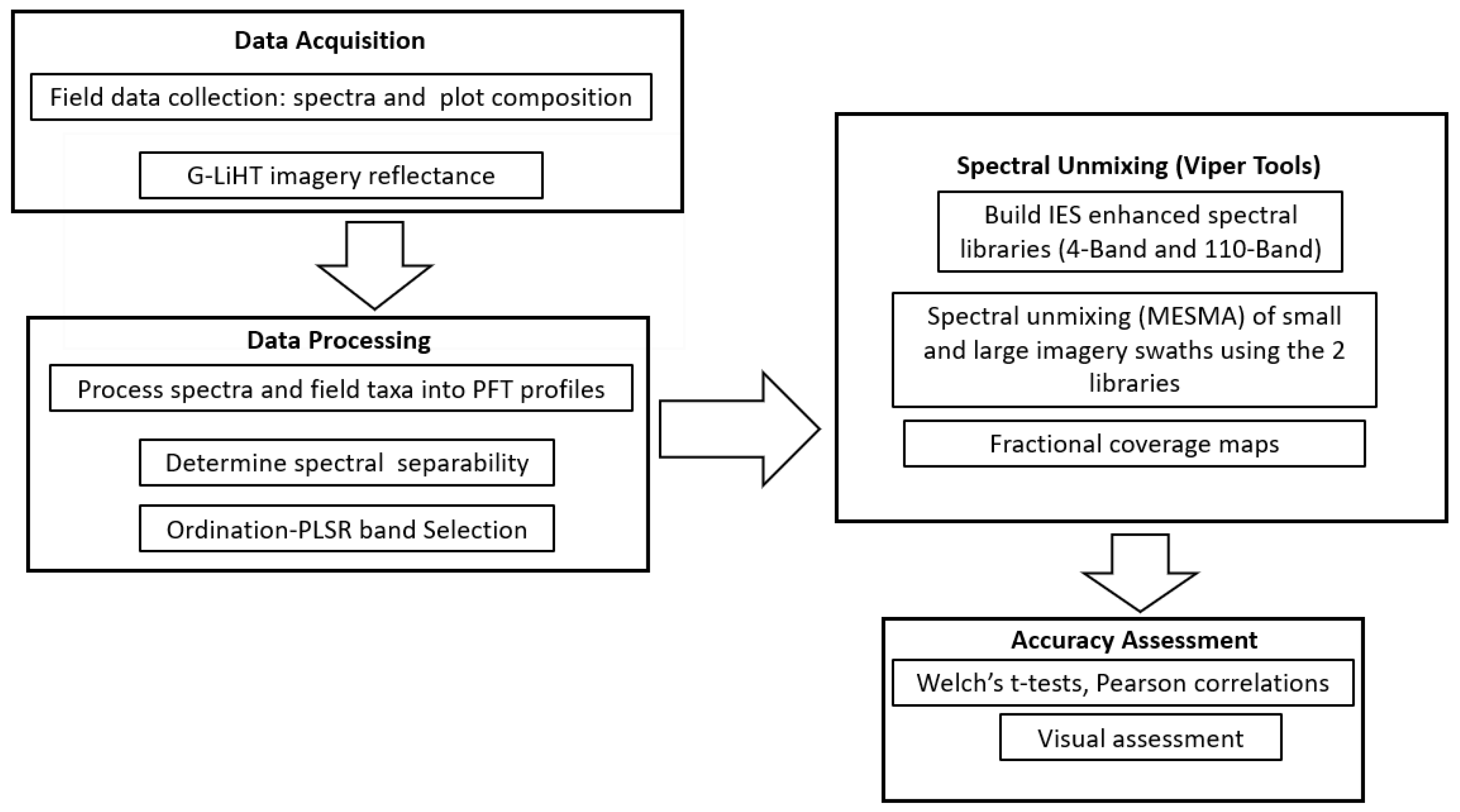
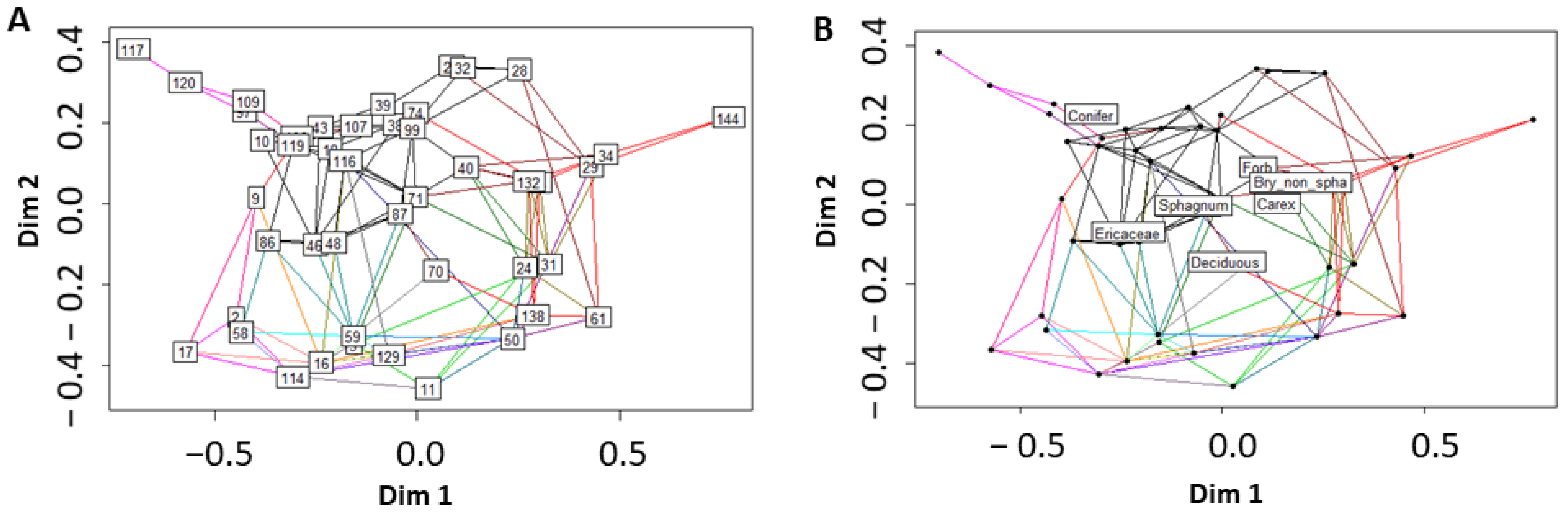
Here, we evaluate the effectiveness of using a field dataset of spectra and plot composition, collected across different wetland classes, to parameterize MESMA models to predict fractional coverage of PFTs. Specific questions include (1) does using combined ordination-partial least squares regression (PLSR) provide an effective feature selection tool for identifying bands for unmixing hyperspectral imagery, (2) can we scale MESMA predictive mapping using the feature selection tool, from a narrow sampled swath to a larger unsampled area, and (3) does constraining MESMA to the verified endmembers present at a site improve prediction of vegetation coverage.
This work complements the existing body of research publications in MESMA such as [16,17,18] in three important ways. First, the field-collected pure spectral libraries of PFT enhance the accuracy of deconvolution of mixed peatland vegetation associations within a single pixel. The second contribution of this work is to demonstrate the use of PLSR as a dimension reduction technique, particularly as applied to vegetation feature extraction and the ability to scale from the small footprint of airborne hyperspectral imagery to the larger footprint of multispectral satellite imagery. Lastly, the focus across multiple wetland classes and hyperspectral tiles, permits the investigation of whether these methods can be used to estimate fractional composition in heterogeneous areas with difficult field access.

2. Materials and Methods

2.1. Study Site

The study sites are wetland-peatlands in the Alaskan Kenai Peninsula’s western lowlands (Figure 1); the westward region of the Peninsula tends toward alpine tundra and grades into wetlands [19,20]. The existing wetland map (EWM) of the Peninsula wetlands [21] is based on a combination of remotely sensed imagery and geomorphology, which categorizes the wetlands into five classes: wet herbaceous, aquatic herbaceous, low shrub, sedge, and black spruce (Figure 2). Our analyses include wet herbaceous, low shrub, sedge, and black spruce wetlands, but do not include the relatively rare and difficult to access aquatic herbaceous wetland.

2.2. Workflow Overview

The research workflow (Figure 3) can be summarized in four main procedural steps. In the field, we collected reflectance and plot composition during a field campaign in August 2019. We used these data to build two spectral reference libraries, one using a small set of PLSR identified bands, and a second using all bands. We use multi-dimensional ordination on field data to characterize floristic composition of wetland classes. We use combined PLSR-ordination, to identify critical bands for separating PFTs. We explore MESMA models’ sensitivity to parameterization by modeling and comparing the outcomes of unmixing: (1) for unmixing imagery when constraining the models by the vegetation known to be present versus unmixing using the full complement of PFTs, and (2) comparing unmixing results of the two spectral libraries. We initially evaluate whether spectral feature selection will result in lower computational times and better classification, by unmixing a small swath, we then scale up to a larger footprint to assess whether the lower computational costs and more accurate mapping hold across larger spatial scales.

2.3. Data Acquisition

We geolocated plots in the field in order to compare with airborne Goddard’s LiDAR Hyperspectral Thermal (G-LiHT) acquisitions. All sites were selected to be within the G-LiHT swath using ArcGIS Online, and the Global Navigation Satellite System (GNSS, Bad Elf Surveyor) to acquire ~1-m geolocation accuracy. We discarded plots having less than 1-m location precision. The field data collection was also constrained to be within a G-LiHT swath that had an accessible wetland. At any one particular site so described, we first located ourselves within the swath, then generated a random number to walk to a starting point where the transect end could be secured. We ran 60-m transects and measured vegetation within a meter square plot, using the point intercept method, every 4–6 m (depending on the geolocation accuracy). We surveyed vegetation composition using line-point intercept methodology [22,23,24,25,26] and identified the dominant plant communities according to the Alaskan Vegetation Classification (AVC) system [27] (Table A1). For the plant functional types, we employed the line-point intercept method [26] of vegetation survey using a 2-m long, 13 mm diameter steel rod marked into upper and lower meters to record vegetation. Presence was recorded as 1 hit per point, per stratum, per taxon for a total of 144 plots. We recorded the vegetation at either the genus or species level depending on our knowledge. Tree samples in this dataset were almost invariably small (<15 cm). Areas with grown Picea mariana, for example, were outside of the wetland sites.
We collected taxa reflectance spectra using an Ocean Optics Flame-S spectrometer in August (2019) to mirror the phenology of the G-LiHT sensor data. The spectrometer samples between 350 and 1000 nm, at a resolution of 1.5 nm (full width half maximum, FWHM). Measurements were made on clear days, within two hours of solar noon, at a height of 0.9 m above ground using 8 fore optic, corresponding to a circular sampling footprint of ~133 cm 2 . To account for changes in ambient light between scans we measured a reflectance standard larger than the sampling footprint prior to each scan (Figure 2B, LabSphere, Spectralon, North Sutton, NH, USA). To improve the signal to noise ratio, we truncated data at both ends of the spectrum, below 400.18 nm, and above 900.21 nm. We visually inspected spectra for noise and subsequently eliminated 4 noisy bands at ~750 nm. Reflectance measurements were converted to ASCII files and imported into R statistical software (Figure 4).
Ground-based spectral measurements were made in homogenous plots, in situ, across multiple wetland classes and include multiple taxa for each PFT profile (Table A2). We refer to the ground spectrometer measurements as the handheld dataset (HHDS) to prevent confusion with G-LiHT spectrometer measurements.
The G-LiHT NASA campaign was flown on 18 and 19 August 2014 (Figure 1). The analyses presented here use three tiles which we refer to using site names Bridge Access Road, Beaver Creek, and Lily Lake (Table 1). G-LiHT data has ~1-m pixel resolution.
G-LiHT’s nominal flying height was 335 m above ground level (AGL); at this altitude, sensor reflectance is a near approximation of surface reflectance. The imaging spectrometer was the Hyperspec (Headwall Photonics, Fitchburg, MA, USA) which operates in the spectral region from 400 nm to 1000 nm with a spectral resolution of 1.5 nm (FWHM), and a spatial resolution of ~1-m [28]. Reflectance products are available on the G-LiHT website (http://glihtdata.gsfc.nasa.gov accessed on 16 September 2019) as orthorectified raster files.
To address the temporal disjunct between field sampling (mid-August 2019) and the initial G-LiHT flyover (mid-August 2014), care was taken to capture field spectral measurements under similar atmospheric, optical, and phenological conditions.

2.4. Data Processing

2.4.1. Plant Functional Type Grouping

PFT is a categorization of vegetation at a more general level than Genus or species and defined by a characteristic feature, e.g., phenology or physiology. There is a robust history of research in combining remote sensing with vegetation mapping at the level of PFTs [29,30,31] and strong support for discriminating between vegetation at the level of PFTs using hyperspectral data [32,33]. Vegetation was identified in the field, to either the family, genus or species level depending on our ability to definitively classify the sample, and then aggregated into PFT (Table 2).
We assess the ability to discriminate between averaged PFT spectral profiles by calculating M-statistics. The M-statistic quantifies the difference between two distributional peaks:
M = m e a n s p e c t r a 1 m e a n s p e c t r a 2 σ 1 + σ 2
where σ is the standard deviation of each distribution. It is useful in its ability to simultaneously compare many narrow bands and identify bands that can be used to discriminate between objects [34]. An M-statistic <1.0 indicates significant overlap between spectral histograms, while an M-statistic >1.0 indicates an ability to discriminate between the distribution curves, i.e., variance within PFT profiles is small relative to variance between profiles [33]. We evaluate separability for three spectral ranges: visible 400–550 nm, red edge position (REP) 680–720 nm, and near infrared (NIR) 721–800 nm.

2.4.2. Ordination and Partial Least Squares Regression (PLSR)

Applying coupled ordination and regression methods to hyperspectral imagery is a well-tested methodology combining field-collected land cover data with remotely sensed spectral data to create sub-pixel floristic gradient mapping [35,36,37,38]. The approach involves first applying ordination to field-sampled plot composition data, to project the composition into multi-axis space describing the plots’ vegetation similarities. The continuous variable resulting from this community mapping describes the gradient of plots’ floristic similarity to one another and often to some expressed or unexpressed underlying environmental gradient such as nutrient availability [39,40]. The PFTs in the gradient can be expressed as centroid values mapped into the multi-ordinate space and occupying a similar position for plots having the same dominant species.
The results of the ordination can be used in PLSR, a matrix regression capable of dealing with the inherent collinearity and redundancy of the numerous narrow bands of hyperspectral imagery [35,36,41,42,43]. We use ordination-regression in this research to understand the covariance between spectra of PFTs collected with the handheld spectrometer, and the class membership of the field plots’ PFTs [44].

2.4.3. Ordination-Isomap Dimensionality Reduction

We use the Isometric Feature Mapping Ordination (IFMO) package Isomap [43,45] to describe community structure in ordinate space [46]. IFMO is a non-linear dimensionality reduction technique used in analyzing floristic data at the site level [47,48]. We selected Bray Curtis as the most appropriate method to describe the plots’ similarity, based on the count method of our field sampling and in agreement with previously published literature [36,49]. Isomap has one free parameter (k) that must be defined and represents the number of nearest neighbors (kNN) for a chosen point. We tune the model for the optimally smallest k parameter with a set of algorithms in the ‘caret’ package [50].

2.4.4. PLSR Relates Spectral Profiles to Isomap Axes

We use PLSR to model the relationship between the peatland vegetation gradient and the spectral data. PLSR is commonly used for spectroscopy applications to reduce the collinearity of data [42,51]. We use the spectral wavelength matrix values as the X-predictor [41,42] and the matrix of PFTs centroid values of the multidimensional community structure ordination as Y-dependent variable. The strength of PLSR lies in its ability to extract underlying salient structure from variables that are noisy, by transferring the information to independent lower dimensional latent variables (LV) to predict the response variable. PLSR has been shown to be well suited to datasets where the number of samples is low [52].
To maximize the PLSR model’s goodness of fit we first narrowed the band selection to the near infrared bands, then applied an iterative backward selection process to the spectral bands using the ‘pls’ [53] and ‘autopls’ packages [37]. The result is a reduced set of spectral bands that can be used as classifiers [44]. We validated the model using leave-one-out (LOO) cross-validation, root mean squared error (RMSE), and the coefficient of correlation R2 for both models.

2.5. MESMA Library and Spectral Unmixing

The fractional coverage of the PFTs was calculated for the G-LiHT imagery using MESMA [17], where the wavelength ( λ ) reflectance mixture M at pixel i is modeled as the sum of the reflectance of the pixel’s reference endmembers (e), weighted by the fractional abundance ( f i k ) of each endmember e of class k ( k = 1 e ) at pixel i, plus a residual term ( ϵ ) equal to the unmodeled portion of the spectrum in pixel i [17,54].
M ( λ ) i = k = 1 e f i k M ( λ ) i k + ϵ ( λ ) i a n d k = 1 e f i k = 1
The optimal model for each pixel i is that which minimizes the root mean square error over all the spectral bands,
R M S E = λ = 1 B ( ϵ ( λ ) i ) 2 / B 1 / 2
where B represents the spectral bands used in unmixing.

2.5.1. Building a Spectral Library

We mapped the 114 G-LiHT bands to their closest match in the 2048 bands of the HHDS, yielding the 110-band set. We imported seventy-two taxa spectra from the HHDS into ENVI for the base library. Endmember variability is a well-documented challenge to building optimal spectral libraries [14]. Sphagnum and conifer endmember variability in the G-LiHT data was greater than the variablility in our HHDS. To adequately capture this variability, we added three profiles extracted from G-LiHT spectra for both conifers and Sphagnum bringing the spectral library to a total of seventy-eight taxa, while forbs’ reflectance could be distinguished in the HHDS, their low presence at all sites (except BAR) meant they could only be clearly identified in the G-LiHT imagery for the wet herbaceous BAR site.
We use iterative endmember selection (IES; [55]) to prune our library to an optimal subset of endmembers. IES selects endmembers iteratively; selecting the subset of spectra that produces the best match as indicated by the highest kappa value. After an initial endmember selection, the next spectrum that results in the best match, in combination with all other spectra in the library, is selected. This process iterates until the match no longer improves. To avoid sub-optimal endmember selection, each endmember in a library is further tested by removing it from the library and determining whether removal also improves the match by increasing the kappa. IES identifies the archetypal endmembers for each PFT. IES has been found to generate libraries with greater unmixing accuracy potential than similar methods like count-based selection (CoB; [56]) and endmember average root mean square error (EAR; [55,56]).
From this IES-pruned library we drew two separate libraries for our imagery unmixing; the full set of 110 bands (the 110-band library) and the four-band library of PLSR identified bands (wavelengths 698 nm, 701 nm, 703 nm, 710 nm).

2.5.2. Spectral Unmixing

We use the IES-pruned libraries to perform MESMA. We first evaluate our model performance in a computationally inexpensive manner, by unmixing small polygons (“small swaths”) encompassing our field sampling transect plots. MESMA generates three products for each pixel: (1) fractional coverage of each PFT in each of the G-LiHT imagery’s pixels (2) Model RMSE for each pixel and (3) per-pixel mapping of model complexity. After this initial computational evaluation and visual confirmation, we apply the unmixing to larger swaths for each G-LiHT tile-site, using the same spectral library and band combinations as used for the smaller swaths.
In addition to the two sets of spectral libraries (110-band and 4-band) we unmixed the pixels using both unconstrained (all the PFTs) and constrained (including only those PFTs confirmed for those pixels).
MESMA was performed with a shade constraint of 0.0 to 0.7; maximum allowable RMSE of 0.025; and a fraction constraint between 0.0 and 1.0. We selected endmember models of shade plus 1, 2, and 3 endmembers. We used Viper Tools [18] for the work building spectral libraries, conducting IES, and performing MESMA. Viper Tools is an IDL-based plugin compatible with ENVI (Harris Geospatial Solutions) Tools 2.0 (https://sites.google.com/site/ucsbviperlab/viper-tools accessed on 10 October 2019).

2.6. Model Fit and Accuracy Assessment

We use three quantitative metrics and a qualitative visual assessment to assess the accuracy of unmixing: We assess the relationship between the arithmetic means of field-sampled plots’ PFTs (reference), and the spectrally unmixed modeled (predicted) plots using Welch’s unequal variance two sample t-tests. To assess the strength of the library, we use Cohen’s kappa coefficients, the MESMA models’ RMSE and their standard deviations which measure fit between the endmember library and the image spectra. We visually assess accuracy of the large swath classification from field data and compare our unmixed wetland classifications to existing wetland maps.
Our t-test statistics include the strength of the correlations (p-value) and the mean difference between the fractional coverages of predicted and sampled plots ( μ value). We expect that the true difference between the reference and fractional coverage means is equal to zero. A positive regression would be consistent with a finding that the modeled population is a good predictor of the field-measured assemblage.

3. Results

3.1. Spectral Separability

Significant separability was observed between all PFTs based on the M-statistic, with the most difficult separability observed between Sphagnum and conifer (Table 3 and Figure 4). The highest M-statistic occurs in the NIR most often.

3.2. Ordination, Isomap Dimensionality Reduction

The vegetation composition of the 144 sampling plots is shown in multi-dimensional ordinate space in (Figure 5A). Plots with identical compositions are only shown once on Figure 4A. At k value of 7 the ordination model retained 30% of the floristic variation. To explore the model sensitivity, we parameterized the model with a range of k values. With the k set to 25, the model retained 81% of the variation. Although using a higher k value has precedent in mapping vegetation distances ([43,57]) the higher k value did not significantly impact our PLSR results, and we chose to model using the optimal k = 7, while the 1st Dimension axis explained the greatest amount of floristic variance (47%), using the first four axes provided significantly more information (94%). In Figure 5B, PFT names represent the average position of that PFT as the dominant taxa in plots, in multi-ordinate space. The full list of 6 dimensions are given in the Appendix A (Table A3).

3.3. Feature Selection: Partial Least Squares Regression Results

Results from PLSR indicate how well the handheld spectral profiles predict the PFTs (Figure 6). The regression identifies four significant latent variable bands (p-value < 0.05); all in the red edge NIR range (Table 3). The PLSR results in a validated R 2 of 0.91 (Table 4) and RMSE of 0.01 for R 2 calibrated set and 0.03 for the R 2 validated set. Only the first ordination dimensions resulted in a significant R 2 . We report only the first axis in our results.

3.4. Calculation of Imagery Endmember Fractional Coverage Using MESMA

The 4-band endmember library (Table 4) and the full 110-band library were used to unmix each of the three small swaths. Unmixing with either library results in 100% unmixed pixels, except BAR where the 110-band model resulted in 98% unmixing (Table 5).
The model fit indicated by lowest RMSE is better for the 4-band library relative to the 110-band library (Table 6). The RMSE indicates how well the library profiles fit the imagery profiles but does not indicate the strength of the classification or provide misclassification information. With the exception of BAR unconstrained unmixing, we find lower processing times using 4 versus 110 bands. The LL computation times were higher than BC and BAR. BAR has low computation times for both the 4-band and 110-band libraries.

3.5. Accuracy Assessment

We compare the average fractional PFTs’ coverage results of the constrained and unconstrained unmixing (predicted fractional coverage), for the 110-bands and the PLSR 4-band sets to the field-sampled fractional coverage (reference fractional coverage), using Welch’s t-tests and boxplots (Figure 7). The boxplots provide a visualization of the results for the difference in means of the reference (sampled) versus predicted coverage. The means cluster more tightly for the 4-band PLSR band unmixing (Figure 7A), while the comparison between the reference and the 110-band unmixing means show greater divergence (Figure 7B). Likewise the constrained versus the unconstrained means are much closer in the PLSR 4-band unmixing than in the 110-band unmixing. Table 6 and Table 7 provide the numerical data supporting the boxplots.
We use Pearson correlation coefficients to further examine the relationship between the average reference and predicted coverages resulting from the spectral unmixing analysis. All comparisons had a strong positive correlation, a finding that supports the idea that the predicted coverage means closely resemble the field-sampled population. We compare the mean difference of these populations and consistently find that the smallest difference between means is shown by the constrained 4-band library (Table 6).
The iterative endmember selection for the libraries results in a higher number of endmembers for the 110-band library (37) and a higher kappa (0.97) than for the 4-band library (24) endmembers and kappa (0.90) (Table 4).
In Figure 8, we display the unmixed buffered transect pixels (“small swaths”) for the BC site showing the fractional PFTs as well as a true color RGB image (Figure 8A). Only the higher density PFTs are shown. From fieldwork and the EWM we know that BC is a Sphagnum dominated Sedge Wetland. Therefore the validity of the unmixing is evidenced by the grey color PFT panels C (graminoid) and E (Sphagnum) being the dominant PFT pixels in the unmixing.
In Figure 9, we show the EWM classification next to the the unmixing for the LL large swath for water, conifer and Sphagnum. These are the dominant classes at this low shrub wetland site. Figure 8 compares the results using the 4-band library to the 110-band library; the 4-band and 110-band images for each class are positioned side-by-side for ease of comparison.

4. Discussion

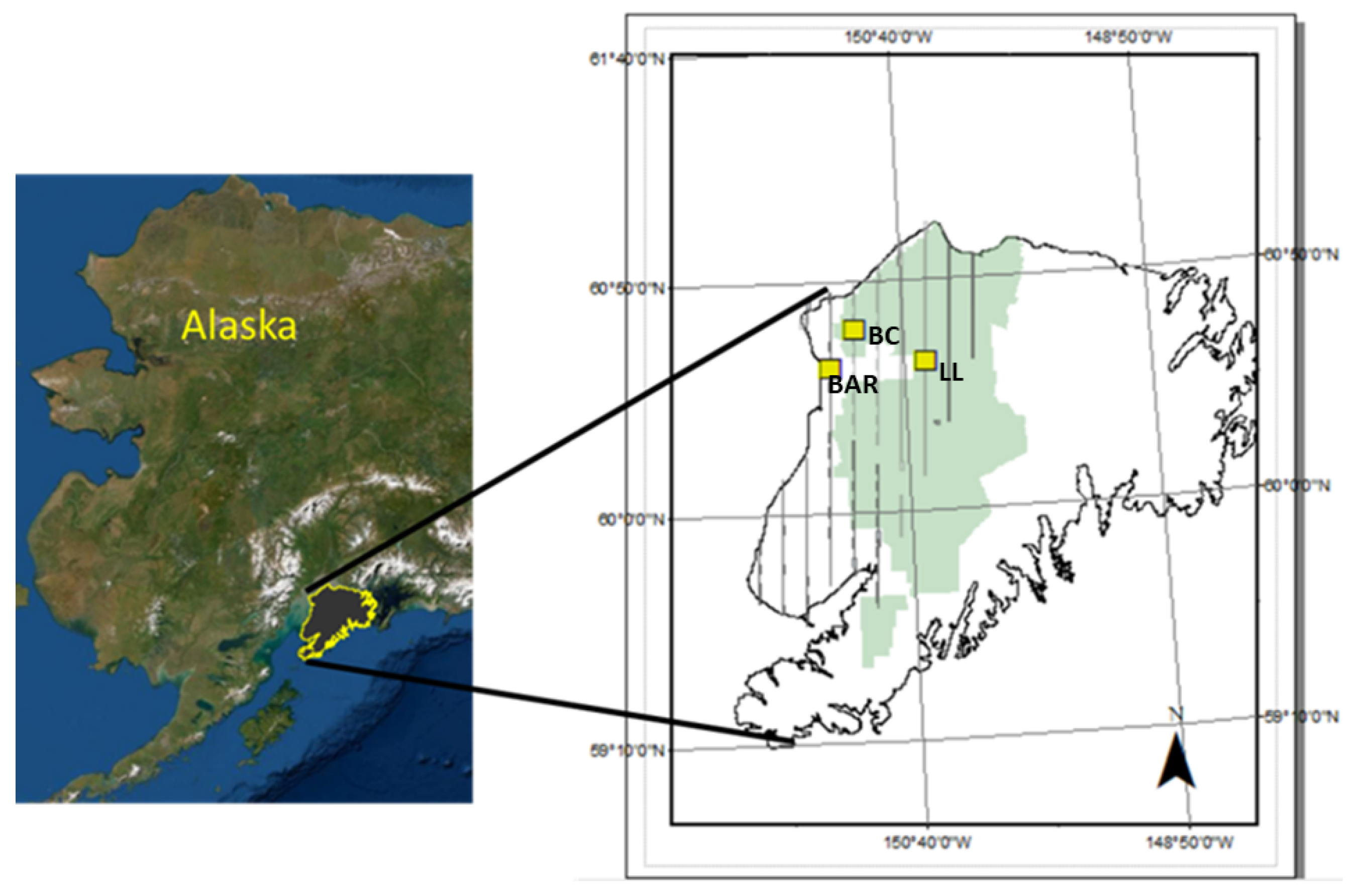
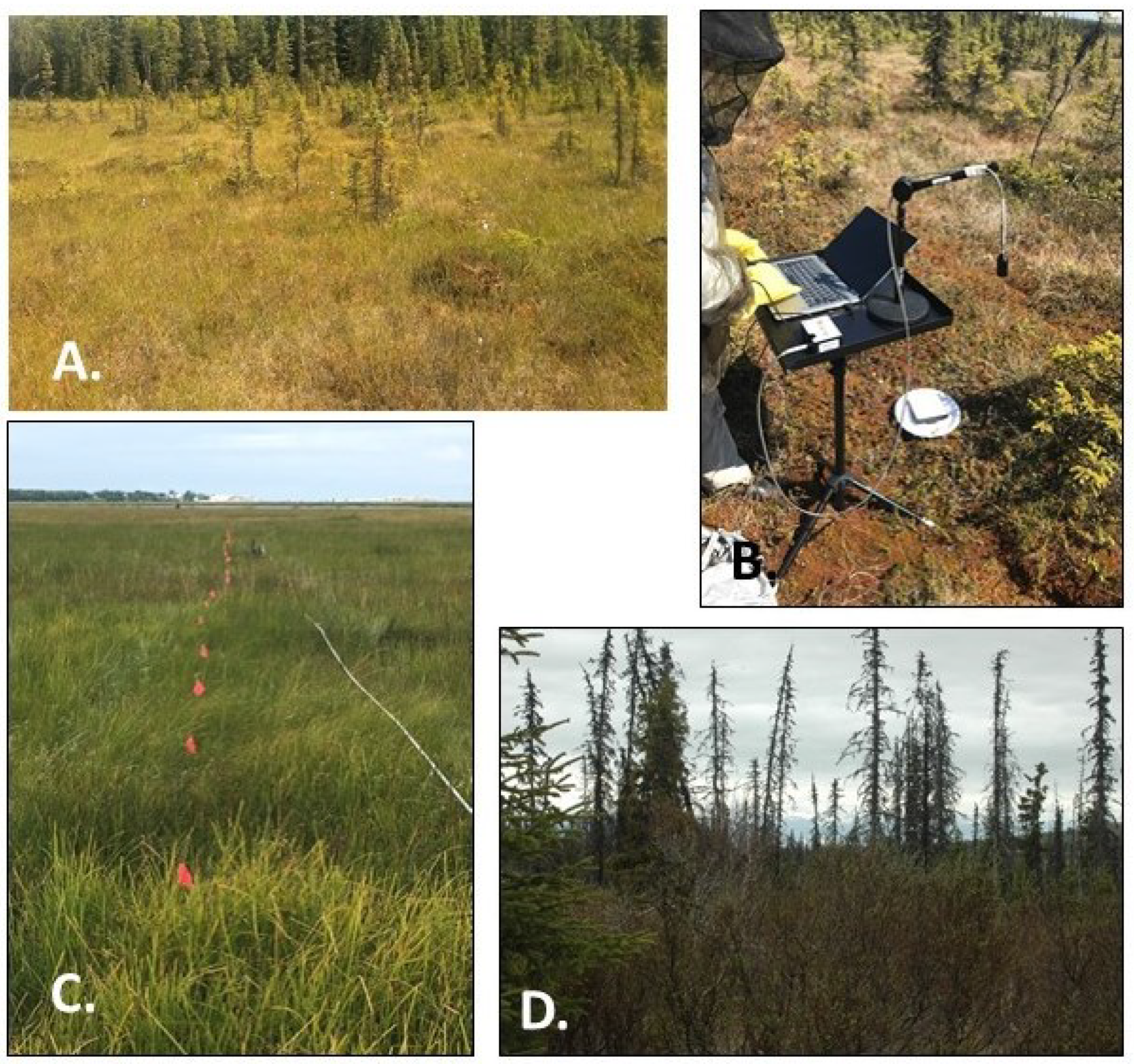
In this research, we integrate field-collected data to create a spectral reference set appropriate for mapping across multiple wetland classes in a suite of subarctic wetland-peatlands. The MESMA mapping that results from the library created from this field data collection suggests that a relatively small investment in fieldwork can be leveraged to map wetlands across multiple hyperspectral tiles.
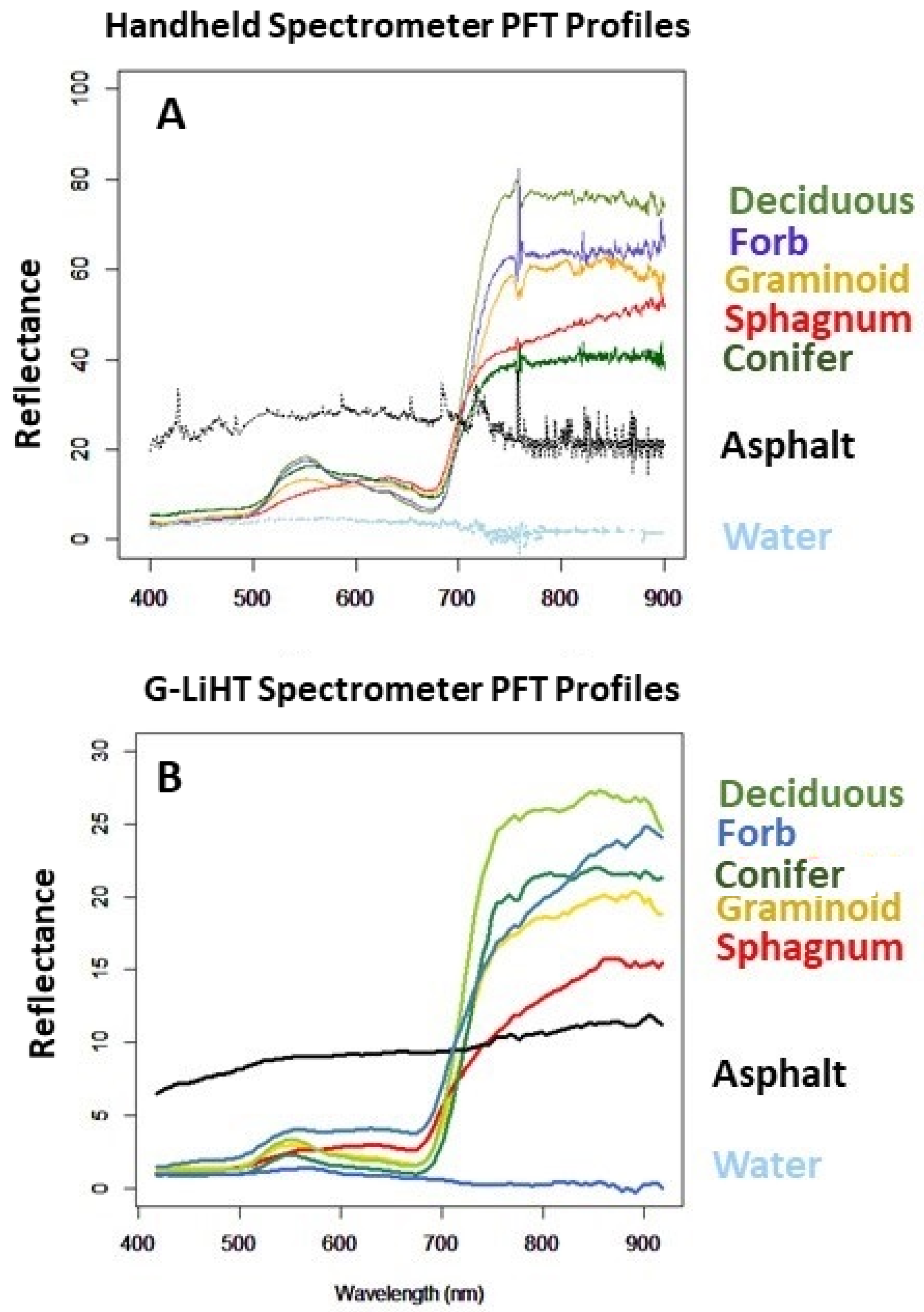
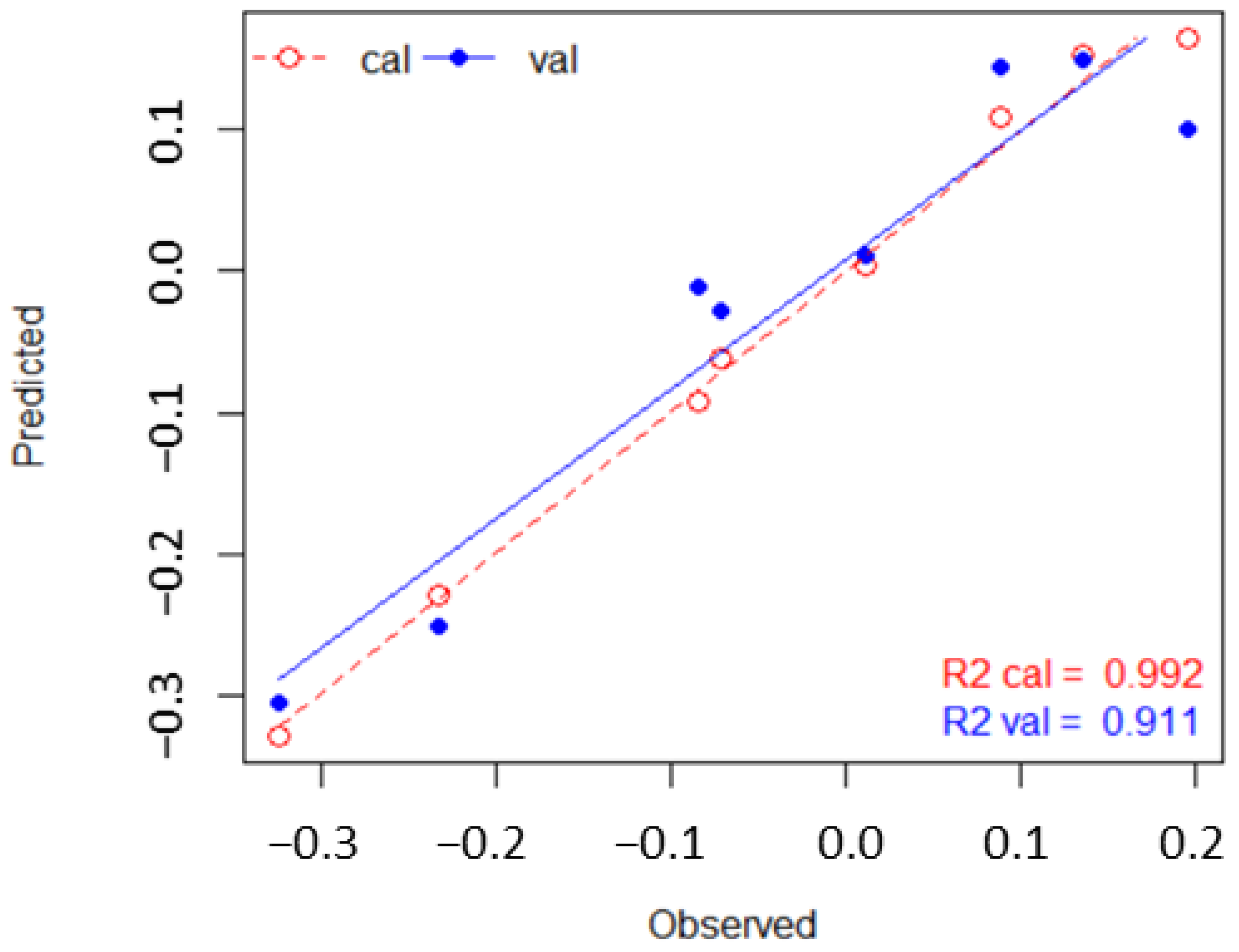
We use a set of study-defined PFT library spectra, to apply PLSR as a feature extraction method to identify a parsimonious set of bands capable of discriminating between PFTs. The four-bands identified through feature extraction can be used in spectral mixture analysis (MESMA) to achieve predictive mapping that appears to have accuracy similar to but with lower classification errors, than that achieved with unmixing using the full set of 110 hyperspectral bands. After unmixing the imagery using MESMA, we find closer correlations between the sampled and the predicted fractional coverages using the PLSR 4-band rather than the 110-band library. These findings agree with previous work on the use of PLSR as a feature selection technique useful in reducing model complexity and to produce more accurate prediction results compared to full wavelength spectrum libraries [58].
With the exception of the Sphagnum category at BAR, we find that while the constrained spectral mixture analysis models returns slightly better results in both model fit and accuracy (i.e., RMSE in Table 5), the unconstrained models’ results are not significantly different. Results in Table 7 also show that the field observed values (column 4) most closely match the Band 64–67 data for most PFT and sites. Agreement between unconstrained and constrained analyses suggests that the predicted species composition based on the unconstrained set of PFTs is relatively close to that predicted by the constrained set of PFTs. Thus, extensive fieldwork in remote wetlands may not be necessary for predicting species composition. Further, when the constrained (columns 6 and 8) and unconstrained (columns 5 and 7) values are similar, it is less important to have extensive field measurements, as it is an indication that unconstrained analysis (with the specified bands, 4 or 110, or both) is sufficient for predictive purposes. This suggests that using unconstrained libraries could be suitable for mapping areas where field sampling is not possible due to inaccessibility.
There is a clear computation cost benefit as a result of using feature extraction to identify critical bands for unmixing. The number of endmembers for subsetting, or in other words the unmixing complexity, is also a significant driver in processing time (Table 8). Some of the matches between predicted and actual are high, an additional indication that the process is robust, while the processing times are small for all small swaths it is greater when we constrained the unmixing by the PFTs known to be present at the site. The processing time for the scaled-up imagery used here increased dramatically and appears to be driven both the number of bands used for unmixing (higher for the higher number of bands) and by the three versus 4-endmember unmixing complexity which is greater for the higher complexity models (Table 8).
In each of the unmixing model results (both the 4-band and 110-band), the PFTs dominating the unmixed swaths are what is anticipated from the wetland class identified using the Alaska Vegetation Classification [27]. The highest fractional coverage correlations between the reference and predicted plots are generally for the 4-band rather than the 110-band models. In other words, for the small swath sampling area of Lily Lake predicted coverage, which is a low shrub-scrub wetland which, according to Viereck [27], would include Sphagnum and woody shrubs, has 58% Sphagnum coverage and 26% woody coverage, with only 13% graminoids. BAR, determined by our field sampling composition to be a Wet Herbaceous wetland, should be dominated by graminoids especially Carex, is 77% graminoid and is close to our plot sampling which found 74% graminoid. Finally, BC which is, according to Viereck, a sedge peatland dominated by Sphagnum and graminoid is 48% Sphagnum and 33% graminoids. Overall, spectral unmixing results in fractional coverages that suggest all three sites are dominated by graminoids and/or Sphagnum. This finding is supported by our field sampling.
Based on the results of the small swath fractional coverages, we suggest it is possible that when Sphagnum is present at a site (as at LL and BC (Table 5)), spectral mixture analysis may over-predict the presence of Sphagnum spp., with the resulting maps displaying a greater fractional coverage than is present. This overprediction may occur because Sphagnum is frequently found at wetland sites as a ground covering such that even when a graminoid or woody taxa are present, they co-occur the Sphagnum, and the woody (or other PFTs) signal is dwarfed by a more dominant Sphagnum signal which may cover a greater percentage of the pixel. We see a related effect when we consider the black spruce occupied wetlands which, according to Viereck, frequently have the spruce appearing together with Sphagnum. In these wetland-peatlands where small spruce often occurs singly and cover only a small meter area, the Sphagnum signal may dominate.
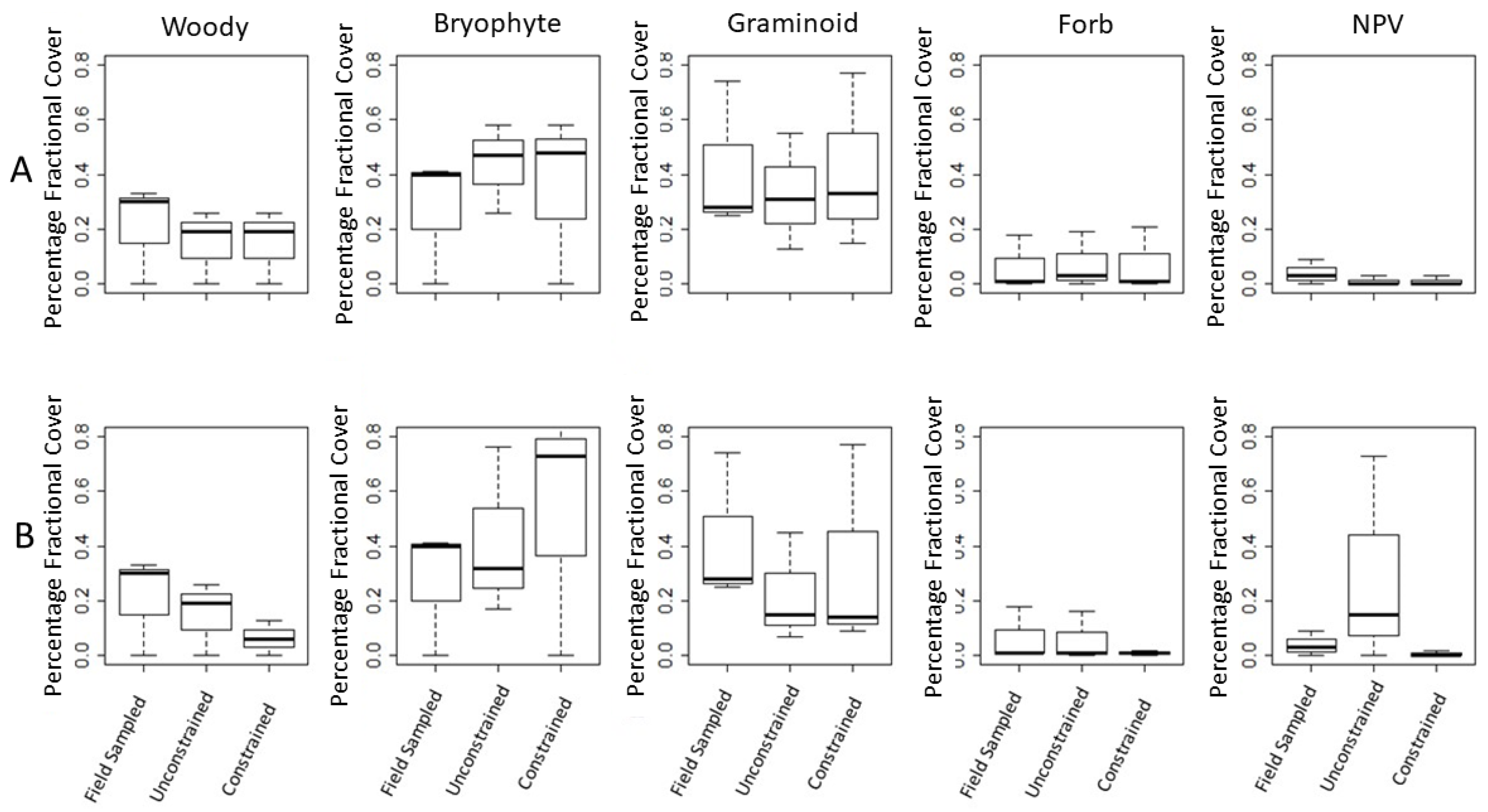
In terms of accuracy assessment, Figure 6 boxplots visually display the finding that fractional coverages’ means, when calculated using a 4-band library for unmixing are closer to field sampled results than means of fractional coverage found using the 110-band library. We further found that constraining PFTs by field-knowledge, did not produce significantly better results suggesting it is more helpful to have a broad locally produced spectral library than it is to have a specific site informed library. The finding makes this feature extraction method meaningful for mapping in areas where field sampling is logistically challenging.
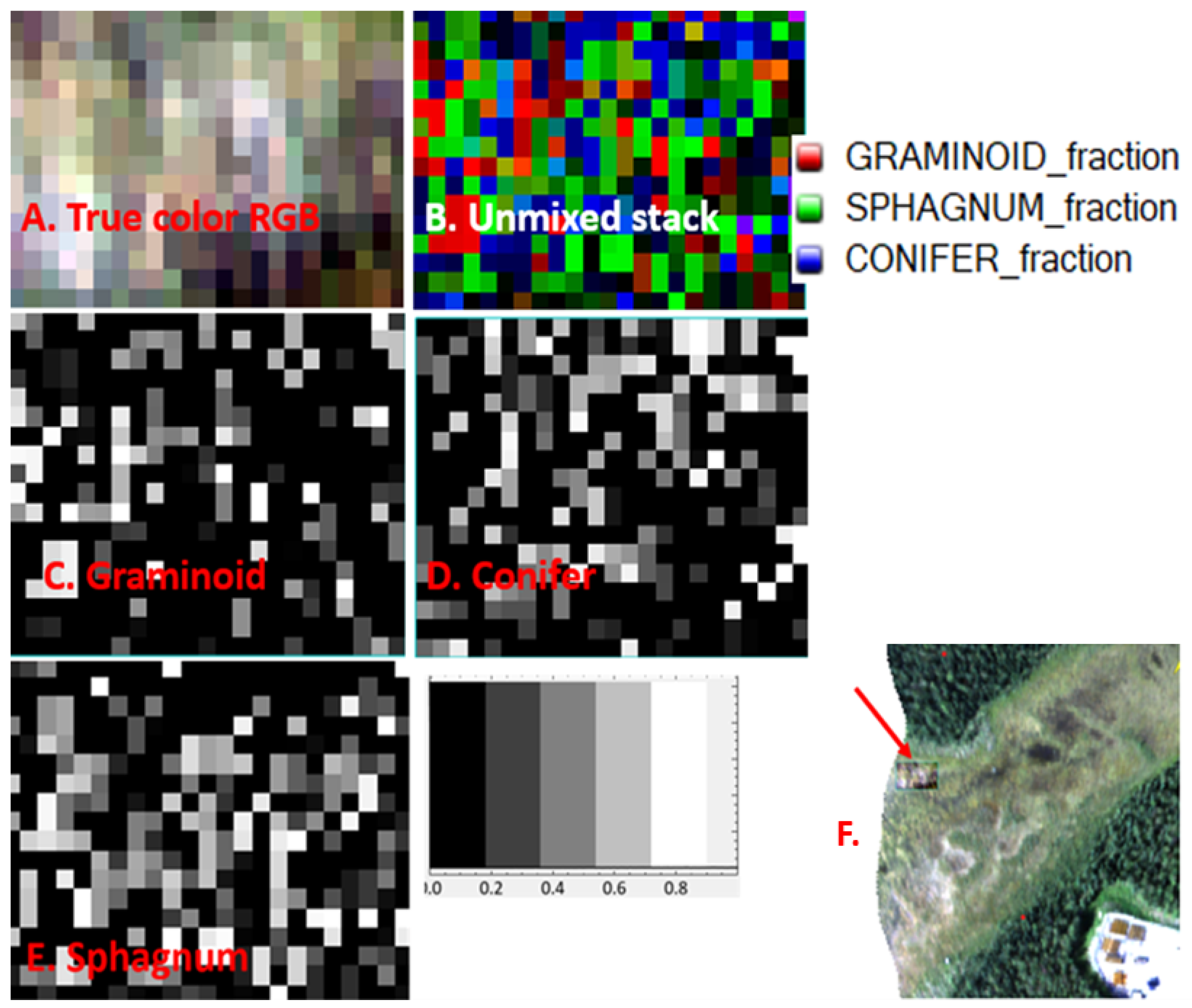
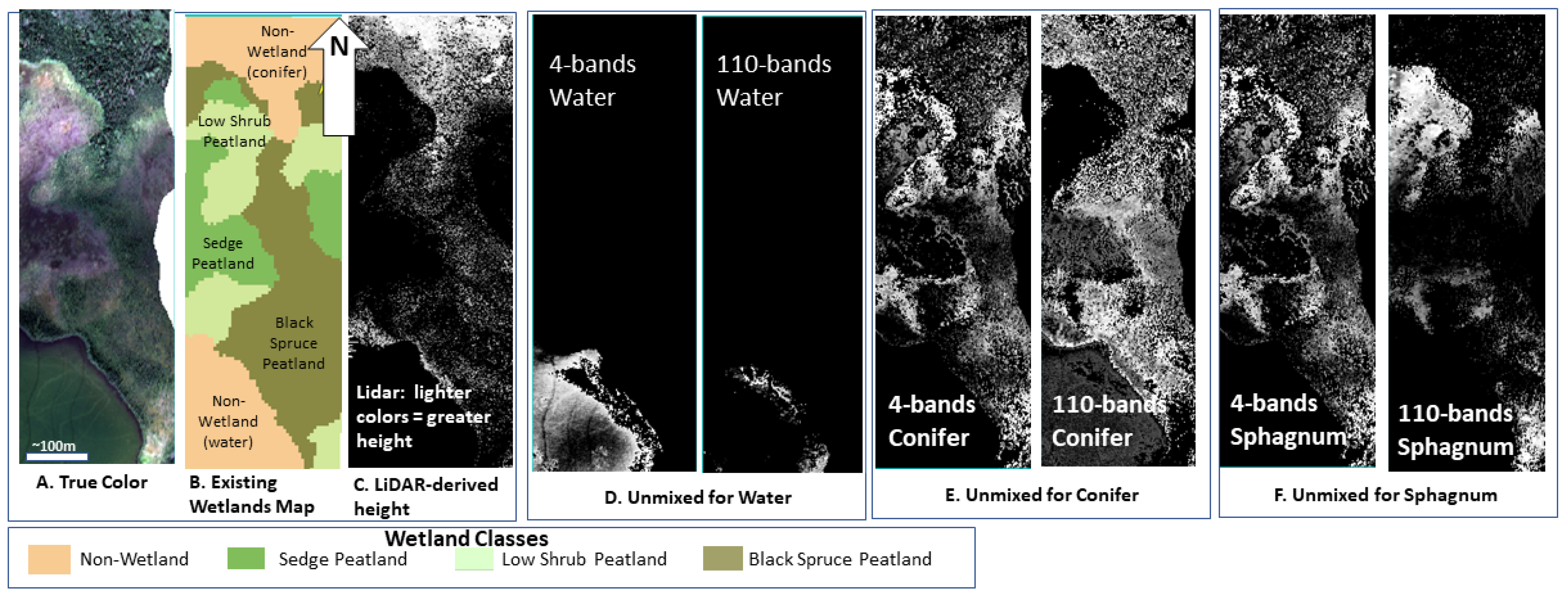
We illustrate scaling up the spectral mixture analysis using a large cropped area from the LL site (Figure 8 and Figure 9). Figure 9A shows the 4-band library successfully unmixing water while the 110-band library does not recognize the full extent of the water and, because the image is close to 100% unmixed, we know the 110-band library is misclassifying water into another class. In Panel B., the 110-band is overclassifying conifers. We see this over-classification by comparing the true-color image with the wetland class overlay, by doing so we see the 110-band library does not follow the wetland class map as closely as does the 4-band library. In Panel C., the 110-band underestimates Sphagnum coverage since we know both from our sampling plots and field-based knowledge, that entire site is underlain by Sphagnum even when conifers are present.
By identifying the small set of bands best able to discriminate between wetland PFTs, this research contributes toward the ability to scale from the high (spatial and spectral) hyperspectral resolution to the lower resolution of multi-spectral imagery. The advantages of scaling from airborne collected hyperspectral imagery to lower spectral resolution of satellite imagery include both the high temporal repeat of satellite imagery and its wall-to-wall, rather than narrow swath, coverage of an area, and the ability to leverage broadly available data.

5. Conclusions

Our findings suggest MESMA can be successful with or without constraining endmembers with a priori knowledge of vegetation, making a significant contribution toward the use of MESMA for inaccessible areas where field sampling cannot be undertaken. Both sets of spectral bands discriminate between PFT but the 4-band unmixing library results in more accurate predictive mapping with lower computational cost. Further, that 4-band unmixing appears to have greater success than 110-band unmixing suggests these methods could be scaled for use with multispectral data. Arctic and subarctic wetland-peatlands are a significant and vulnerable part of the global system. This study and the implications and potential for multispectral analysis without extensive field campaigns demonstrate that the work can be scaled up to a wide regional analysis of sub-arctic wetlands.

Author Contributions

Conceptualization, J.M.R. and H.C.; methodology, H.C. and J.M.R.; software, H.C.; validation, H.C., J.M.R. and D.M.; formal analysis, all authors.; investigation, H.C.; resources, J.M.R.; data curation, H.C.; writing—original draft preparation, H.C.; writing—review and editing, all authors.; visualization, H.C., J.M.R. and S.C.P.; supervision, J.M.R. and S.C.P.; project administration, J.M.R.; funding acquisition, J.M.R., H.C. and D.M. All authors have read and agreed to the published version of the manuscript.

Funding

This research was funded by the Lehigh University Presidential Fellowship, Earth and Environmental Sciences Department, and a Lehigh University Faculty Innovation Grant. In-field logistical support was provided by the US Fish and Wildlife Service.

Data Availability Statement

G-LiHT data are available from NASA at https://gliht.gsfc.nasa.gov accessed on 3 January 2023. Please contact the corresponding author with requests for handheld spectral profiles.

Acknowledgments

This research would not have been possible without the support of John Morton and the staff of the Kenai National Wildlife Refuge and Lehigh University. The authors would also like to thank Hans-Erik Andersen of the U.S. Forest Service; Bruce Cook, NASA; Benjamin Felzer and Robert Booth, Lehigh University; Mike Gracz; Kevin Fisher, and Dar Roberts. The findings and conclusions in this article are those of the authors and do not necessarily represent the views of the U.S. Fish and Wildlife Service.

Conflicts of Interest

The authors declare no conflict of interest. The funders had no role in the design of the study; in the collection, analyses, or interpretation of data; in the writing of the manuscript; or in the decision to publish the results.

Abbreviations

The following abbreviations are used in this manuscript:
AGLAbove ground level
AVCAlaskan Vegetation Classification
BARBridge Access Road
BCBeaver Creek
CoBCount-based selection
EAREndmember average root mean square error
ENVIEnvironment for Visualizing Images
EWMExisting Wetland Map
FWHMFull Width Half Maximum
G-LiHTGoddard’s LiDAR Hyperspectral Thermal Imager
HHDSHandheld Data Set
IESIterative Endmember Selection
IFMOIsometric Feature Mapping Ordination
LLLily Lake
LOOLeave One Out
LVLatent Variables
MDPIMultidisciplinary Digital Publishing Institute
MESMAMultiple Endmember Spectral Mixture Analysis
MIROC-ES2LModel for Interdisciplinary Research on Climate,
 Earth System version 2 for Long-term
NIRNear infrared
NPVNon photosynthetic vegetation
PFTPlant Functional Type
PLSRPartial Least Squares Regression
REPRed Edge Position
RMSERoot Mean Square Error
SMASpectral Mixture Analysis

Appendix A

Table A1. Comparison between the Alaskan Vegetation Classification (AVC, [27] of the sampled wetland-peatlands and the Existing Wetland Map [21]. For full detail see [27].
AVC Level IAVC Level IIAVC Level IIIAVC Level IVTaxa in This AVC LevelEWM ClassSite (This Study)
I. ForestA. Needleleaf(2) Open needleleaf woodland (canopy 10-25 percent)d. Black spruce on wet boggy sites, often with Sphagnum mossesPicea mariana; P. glauca; Alnus crispa; Betula glandulosa; Pleurozium schreberei; Rubus camaemorus; edum decumbens; Vaccinium spp.Black Spruce PeatlandBeaver Creek, Transect 2
II. ScrubC. Low scrub(1) Open low scrube. Shrub birch-ericaceous shrub bogsLedub decumbens; Sphagnum spp.; Emepetrian nigrum; Kalmia polifolia; Andromeda polifolia; Vaccinium vitis idaeaLow Shrub PeatlandLily Lake
III. HerbaceousA. Graminoid(3) Wet graminoid herbaceousk. Subarctic lowland sedge-moss bog meadowCarex aquatilis, Sphagnum spp. Eriophorum russeolum, Equisetum fluvatileSedge PeatlandBeaver Creek, Transect 1
III. HerbaceousA. Graminoid(3) Wet graminoid herbaceousf. Subarctic lowland herb wet meadowCarex spp.Wet Herbaceous PeatlandBridge Access Road
Table A2. Number of spectral profiles for each Plant Functional Type, and from which wetland classes.
TaxaProfiles MeasuredWetland-Peatland Type from Which Spectra Were Collected
Sphagnum6Low shrub peatland, Sedge peatland
Forbs6Wet herbaceous peatland
Conifer7Low shrub peatland, Black spruce peatland
Deciduous6Low shrub peatland, Sedge peatland
Carex6Low shrub peatland, Sedge peatland
Ericaceae6Sedge peatland, Black spruce peatland
Poaceae6Wet herbaceous peatland
Table A3. Species scores from Isomap for the first six dimensions (Vectors “V” from 1 to 6, of the handheld dataset (HHDS).
SpeciesV1V2V3V4V5V6
Deciduous0.01−0.14−0.040.05−0.02−0.01
Carex0.140.00−0.01−0.010.02−0.02
Forb0.090.090.100.04−0.07−0.07
Bryophyte non-Sphagnum0.190.06−0.07−0.11−0.080.00
Poaceae−0.08−0.01−0.100.110.030.07
Ericaceae−0.23−0.070.02−0.03−0.010.02
Conifer−0.320.230.03−0.120.090.00
Sphagnum−0.070.00−0.020.010.000.00

References

  1. Fenner, N.; Freeman, C. Drought-induced carbon loss in peatlands. 895. Nat. Geosci. 2011, 4, 895–896. [Google Scholar] [CrossRef]
  2. Lange, M.; Eisenhauer, N.; Sierra, C.A.; Bessler, H.; Engels, C.; Griffiths, R.I.; Mellado-Vázquez, P.G.; Malik, A.A.; Roy, J.; Scheu, S.; et al. Plant diversity increases soil microbial activity and soil carbon storage. Nat. Commun. 2015, 6, 6707. [Google Scholar] [CrossRef] [Green Version]
  3. Luthin, J.; Guymon, G. Soil moisture-vegetation-temperature relationships in central Alaska. J. Hydrol. 1974, 23, 233–246. [Google Scholar] [CrossRef]
  4. Cleve, K.V.; Yarie, J. Interaction of temperature, moisture, and soil chemistry in controlling nutrient cycling and ecosystem development in the taiga of Alaska. In Forest Ecosystems in the Alaskan Taiga; Springer: Berlin/Heidelberg, Germany, 1986; pp. 160–189. [Google Scholar]
  5. Hobbie, S.; Schimel, J.; Trumbore, S.; Randerson, J. A mechanistic understanding of carbon storage and turnover in high-latitude soil. Glob. Chang. Biol. 2000, 6, 196–210. [Google Scholar] [CrossRef] [Green Version]
  6. Limpens, J.; Berendse, F.; Blodau, C.; Canadell, J.; Freeman, C.; Holden, J.; Roulet, N.; Rydin, H.; Schaepman-Strub, G. Peatlands and the carbon cycle: From local processes to global implications—A synthesis. Biogeosciences 2008, 5, 1475–1491. [Google Scholar] [CrossRef] [Green Version]
  7. Tang, J.; Miller, P.A.; Persson, A.; Olefeldt, D.; Pilesjö, P.; Heliasz, M.; Jackowicz-Korczynski, M.; Yang, Z.; Smith, B.; Callaghan, T.V.; et al. Carbon budget estimation of a subarctic catchment using a dynamic ecosystem model at high spatial resolution. Biogeosciences 2015, 12, 2791–2808. [Google Scholar] [CrossRef] [Green Version]
  8. Malhotra, A.; Brice, D.J.; Childs, J.; Graham, J.D.; Hobbie, E.A.; Vander Stel, H.; Feron, S.C.; Hanson, P.J.; Iversen, C.M. Peatland warming strongly increases fine root growth. Proc. Natl. Acad. Sci. USA 2020, 117, 17627–17634. [Google Scholar] [CrossRef]
  9. Hajima, T.; Watanabe, M.; Yamamoto, A.; Tatebe, H.; Noguchi, M.A.; Abe, M.; Ohgaito, R.; Ito, A.; Yamazaki, D.; Okajima, H.; et al. Development of the MIROC-ES2L Earth system model and the evaluation of biogeochemical processes and feedbacks. Geosci. Model Dev. 2020, 13, 2197–2244. [Google Scholar] [CrossRef]
  10. Keshava, N.; Mustard, J. Spectral Unmixing. IEEE Signal Process Mag. 2002, 19, 44. [Google Scholar] [CrossRef]
  11. Wetherley, E.B.; Roberts, D.A.; McFadden, J.P. Mapping spectrally similar urban materials at sub-pixel scales. Remote Sens. Environ. 2017, 195, 170–183. [Google Scholar] [CrossRef]
  12. Lantz, T.C.; Gergel, S.E.; Kokelj, S.V. Spatial heterogeneity in the shrub tundra ecotone in the Mackenzie Delta region, Northwest Territories: Implications for Arctic environmental change. Ecosystems 2010, 13, 194–204. [Google Scholar] [CrossRef]
  13. Adams, J.B.; Smith, M.O.; Johnson, P.E. Spectral mixture modeling: A new analysis of rock and soil types at the Viking Lander 1 site. J. Geophys. Res. Solid Earth 1986, 91, 8098–8112. [Google Scholar] [CrossRef]
  14. Somers, B.; Asner, G.P.; Tits, L.; Coppin, P. Endmember variability in spectral mixture analysis: A review. Remote Sens. Environ. 2011, 115, 1603–1616. [Google Scholar] [CrossRef]
  15. Fangju, W. Fuzzy supervised classification of remotely sensing images. IEEE Trans. Geosci. Remote Sens. 1999, 28, 194–201. [Google Scholar]
  16. Roberts, D.A.; Gardner, M.E.; Church, R.; Ustin, S.L.; Green, R.O. Optimum strategies for mapping vegetation using multiple-endmember spectral mixture models. In Imaging Spectrometry III; SPIE: Bellingham, WA, USA, 1997; Volume 3118, pp. 108–119. [Google Scholar]
  17. Roberts, D.A.; Gardner, M.; Church, R.; Ustin, S.; Scheer, G.; Green, R. Mapping chaparral in the Santa Monica Mountains using multiple endmember spectral mixture models. Remote Sens. Environ. 1998, 65, 267–279. [Google Scholar] [CrossRef]
  18. Roberts, D.; Halligan, K.; Dennison, P.; Dudley, K.; Somers, B.; Crabbé, A. VIPER TOOLS. 2017. Available online: https://sites.google.com/site/ucsbviperlab/viper-tools (accessed on 10 October 2019).
  19. Karlstrom, T.N. Quaternary Geology of the Kenai Lowland and Glacial History of the Cook Inlet Region, Alaska; Technical Report; US Government Printing Office: Washington, DC, USA, 1964. [Google Scholar]
  20. Magness, D.R.; Morton, J.M. Using climate envelope models to identify potential ecological trajectories on the Kenai Peninsula, Alaska. PLoS ONE 2018, 13, e0208883. [Google Scholar] [CrossRef] [Green Version]
  21. Gracz, M.; Noyes, K.; North, P.; Tande, G. Wetland Mapping and Classification of the Kenai Lowland, Alaska. 2008. Available online: http://www.kenaipeatlands.net/ (accessed on 10 March 2019).
  22. Jonasson, S. Evaluation of the point intercept method for the estimation of plant biomass. Oikos 1988, 52, 101–106. [Google Scholar] [CrossRef]
  23. Caratti, J.F. The LANDFIRE prototype project reference database. In The LANDFIRE Prototype Project: Nationally Consistent and Locally Relevant Geospatial Data for Wildland Fire Management Gen. Tech. Rep. RMRS-GTR-175; Matthew, G.R., Christine, K.F., Eds.; US Department of Agriculture, Forest Service, Rocky Mountain Research Station: Fort Collins, CO, USA, 2006; Volume 175, pp. 69–98. [Google Scholar]
  24. Schaepman-Strub, G.; Limpens, J.; Menken, M.; Bartholomeus, H.; Schaepman, M.E. Towards spatial assessment of carbon sequestration in peatlands: Spectroscopy based estimation of fractional cover of three plant functional types. Biogeosciences 2009, 6, 275–284. [Google Scholar] [CrossRef] [Green Version]
  25. Bonham, C.D. Measurements for Terrestrial Vegetation; John Wiley & Sons: New York, NY, USA, 2013. [Google Scholar]
  26. Rochefort, L.; Isselin-Nondedeu, F.; Boudreau, S.; Poulin, M. Comparing survey methods for monitoring vegetation change through time in a restored peatland. Wetl. Ecol. Manag. 2013, 21, 71–85. [Google Scholar] [CrossRef]
  27. Viereck, L.; Dyrness, C.; Batten, A.; Wenzlick, K. The Alaska Vegetation Classification; USDA Forest Service General Technical Report PNW-GTR-286; Pacific Northwest Research Station: Portland, OR, USA, 1992. [Google Scholar]
  28. Cook, B.D.; Corp, L.A.; Nelson, R.F.; Middleton, E.M.; Morton, D.C.; McCorkel, J.T.; Masek, J.G.; Ranson, K.J.; Ly, V.; Montesano, P.M. NASA Goddard’s LiDAR, hyperspectral and thermal (G-LiHT) airborne imager. Remote Sens. 2013, 5, 4045–4066. [Google Scholar] [CrossRef] [Green Version]
  29. DeFries, R.S.; Field, C.B.; Fung, I.; Justice, C.O.; Los, S.; Matson, P.A.; Matthews, E.; Mooney, H.A.; Potter, C.S.; Prentice, K.; et al. Mapping the land surface for global atmosphere-biosphere models: Toward continuous distributions of vegetation’s functional properties. J. Geophys. Res. Atmos. 1995, 100, 20867–20882. [Google Scholar] [CrossRef]
  30. Ustin, S.L.; Gamon, J.A. Remote sensing of plant functional types. Remote Sens. Plant Funct. Types New Phytol. 2010, 186, 795–816. [Google Scholar] [CrossRef]
  31. Schweiger, A.K.; Schütz, M.; Risch, A.C.; Kneubühler, M.; Haller, R.; Schaepman, M.E. How to predict plant functional types using imaging spectroscopy: Linking vegetation community traits, plant functional types and spectral response. Methods Ecol. Evol. 2017, 8, 86–95. [Google Scholar] [CrossRef]
  32. Cole, B.; McMorrow, J.; Evans, M. Spectral monitoring of moorland plant phenology to identify a temporal window for hyperspectral remote sensing of peatland. ISPRS J. Photogramm. Remote Sens. 2014, 90, 49–58. [Google Scholar] [CrossRef]
  33. Rebelo, A.J.; Somers, B.; Esler, K.J.; Meire, P. Can wetland plant functional groups be spectrally discriminated? Remote Sens. Environ. 2018, 210, 25–34. [Google Scholar] [CrossRef]
  34. Kaufman, Y.J.; Remer, L.A. Detection of forests using mid-IR reflectance: An application for aerosol studies. IEEE Trans. Geosci. Remote Sens. 1994, 32, 672–683. [Google Scholar] [CrossRef]
  35. Schmidtlein, S.; Sassin, J. Mapping of continuous floristic gradients in grasslands using hyperspectral imagery. Remote Sens. Environ. 2004, 92, 126–138. [Google Scholar] [CrossRef]
  36. Feilhauer, H.; Faude, U.; Schmidtlein, S. Combining Isomap ordination and imaging spectroscopy to map continuous floristic gradients in a heterogeneous landscape. Remote Sens. Environ. 2011, 115, 2513–2524. [Google Scholar] [CrossRef]
  37. Schmidtlein, S.; Feilhauer, H.; Bruelheide, H. Mapping plant strategy types using remote sensing. J. Veg. Sci. 2012, 23, 395–405. [Google Scholar] [CrossRef]
  38. Neumann, C.; Weiss, G.; Schmidtlein, S.; Itzerott, S.; Lausch, A.; Doktor, D.; Brell, M. Gradient-based assessment of habitat quality for spectral ecosystem monitoring. Remote Sens. 2015, 7, 2871–2898. [Google Scholar] [CrossRef] [Green Version]
  39. Austin, M.P. Continuum concept, ordination methods, and niche theory. Annu. Rev. Ecol. Syst. 1985, 16, 39–61. [Google Scholar] [CrossRef]
  40. Middleton, M.; Närhi, P.; Arkimaa, H.; Hyvönen, E.; Kuosmanen, V.; Treitz, P.; Sutinen, R. Ordination and hyperspectral remote sensing approach to classify peatland biotopes along soil moisture and fertility gradients. Remote Sens. Environ. 2012, 124, 596–609. [Google Scholar] [CrossRef]
  41. Wold, S.; Martens, H.; Wold, H. The multivariate calibration problem in chemistry solved by the PLS method, in Matrix pencils. In Matrix Pencils; Kågström, B., Ruhe, A., Eds.; Springer: Berlin/Heidelberg, Germany, 1983; Volume 973, pp. 286–293. [Google Scholar]
  42. Wold, S.; Sjöström, M.; Eriksson, L. PLS-regression: A basic tool of chemometrics. Chemom. Intell. Lab. Syst. 2001, 58, 109–130. [Google Scholar] [CrossRef]
  43. Harris, A.; Charnock, R.; Lucas, R. Hyperspectral remote sensing of peatland floristic gradients. Remote Sens. Environ. 2015, 162, 99–111. [Google Scholar] [CrossRef] [Green Version]
  44. Roth, K.L.; Roberts, D.A.; Dennison, P.E.; Alonzo, M.; Peterson, S.H.; Beland, M. Differentiating plant species within and across diverse ecosystems with imaging spectroscopy. Remote Sens. Environ. 2015, 167, 135–151. [Google Scholar] [CrossRef]
  45. Tenenbaum, J.B.; de Silva, V.; Langford, J.C. A Global Geometric Framework for Nonlinear Dimensionality Reduction. Science 2000, 290, 2319–2323. [Google Scholar] [CrossRef]
  46. Oksanen, J.; Blanchet, F.G.; Kindt, R.; Legendre, P.; Minchin, P.R.; O’Hara, R.B.; Wagner, H. Package Vegan. Community Ecology Package. R Package Vegan, Vers 2.3-1; R Core Team: Vienna, Austria, 2013. [Google Scholar]
  47. Mahecha, M.D.; Martínez, A.; Lischeid, G.; Beck, E. Nonlinear dimensionality reduction: Alternative ordination approaches for extracting and visualizing biodiversity patterns in tropical montane forest vegetation data. Ecol. Inform. 2007, 2, 138–149. [Google Scholar] [CrossRef]
  48. Mahecha, M.D.; Schmidtlein, S. Revealing biogeographical patterns by nonlinear ordinations and derived anisotropic spatial filters. Glob. Ecol. Biogeogr. 2008, 17, 284–296. [Google Scholar] [CrossRef]
  49. Unberath, I.; Vanierschot, L.; Somers, B.; Van De Kerchove, R.; Vanden Borre, J.; Unberath, M.; Feilhauer, H. Remote sensing of coastal vegetation: Dealing with high species turnover by mapping multiple floristic gradients. Appl. Veg. Sci. 2019, 22, 534–546. [Google Scholar] [CrossRef]
  50. Kuhn, M. Building predictive models in R using the caret package. J. Stat. Softw. 2008, 28, 1–26. [Google Scholar] [CrossRef] [Green Version]
  51. Balabin, R.M.; Smirnov, S.V. Variable selection in near-infrared spectroscopy: Benchmarking of feature selection methods on biodiesel data. Anal. Chim. Acta 2011, 692, 63–72. [Google Scholar] [CrossRef]
  52. Geladi, P.; BR, K. Partial least-squares regression—A tutorial. Anal. Chim. Acta 1986, 185, 1–17. [Google Scholar] [CrossRef]
  53. Mevik, B.H.; Wehrens, R.; Liland, K.H. Pls: Partial Least Squares and Principal Component Regression. R Package Version 2.7-3. 2020. Available online: https://CRAN.R-project.org/package=pls (accessed on 16 October 2019).
  54. Bogan, S.A.; Antonarakis, A.S.; Moorcroft, P.R. Imaging spectrometry-derived estimates of regional ecosystem composition for the Sierra Nevada, California. Remote Sens. Environ. 2019, 228, 14–30. [Google Scholar] [CrossRef]
  55. Roth, K.L.; Dennison, P.E.; Roberts, D.A. Comparing endmember selection techniques for accurate mapping of plant species and land cover using imaging spectrometer data. Remote Sens. Environ. 2012, 127, 139–152. [Google Scholar] [CrossRef]
  56. Dennison, P.E.; Roberts, D.A. Endmember selection for multiple endmember spectral mixture analysis using endmember average RMSE. Remote Sens. Environ. 2003, 87, 123–135. [Google Scholar] [CrossRef]
  57. Böttcher, S.; Merz, C.; Lischeid, G.; Dannowski, R. Using Isomap to differentiate between anthropogenic and natural effects on groundwater dynamics in a complex geological setting. J. Hydrol. 2014, 519, 1634–1641. [Google Scholar] [CrossRef]
  58. Liu, T.; Xu, T.; Yu, F.; Yuan, Q.; Guo, Z.; Xu, B. A method combining ELM and PLSR (ELM-P) for estimating chlorophyll content in rice with feature bands extracted by an improved ant colony optimization algorithm. Comput. Electron. Agric. 2021, 186, 106177. [Google Scholar] [CrossRef]
Figure 1. A map of Alaska (left) with the Kenai Peninsula outlined in yellow. On the right, the map of the Kenai Peninsula shows the National Wildlife Refuge (green), the 2014 flight campaign of NASA Goddard’s LiDAR Hyperspectral Thermal mission(G-LiHT) (grey bars), and the approximate location of the three sampling sites (BAR, Bridge Access Road; BC, Beaver Creek; LL, Lily Lake) referenced in this research (yellow boxes).
Remotesensing 15 01440 g001
Figure 2. Images illustrating the four wetland classes sampled for this research. (A). Sedge Peatland (Beaver Creek) (B). Low Shrub (Lily Lake) with the spectrometer set up (C). Wet Herbaceous (Bridge Access Road) with transect flags (D). Black spruce.
Remotesensing 15 01440 g002
Figure 3. Synoptic workflow illustrates the four main procedural steps: Data Acquisition, Data Processing, Spectral Unmixing, Accuracy Assessment.
Remotesensing 15 01440 g003
Figure 4. Spectral curves of PFT taken at Kenai wetland sites. (A). Averaged curves taken with a handheld spectrometer. (B). Spectral curves for each PFT, gathered from G-LiHT imagery pixels, shown here as a comparison to the handheld measurements.
Remotesensing 15 01440 g004
Figure 5. Matrix Results for Dimensions 1 and 2 from Multi-Dimensional Ordination. Both (A,B) show Isomap Distances for k = 7, Plots = 144, PFT = 8. (A) Numbered-rectangles represent composition of plots sampled in the field. More similar plot compositions are indicated by closer rectangles and more similar line coloring. For plots with the same or highly similar composition, only one rectangle is visible. (B) for the same sampled plots as (A), rectangles show the dominant PFT as centroids in multi-ordinate space.
Remotesensing 15 01440 g005
Figure 6. Regression lines from PLSR show how spectra from handheld measurements (Observed) predict PFT class membership (Predicted) with high accuracy (0.911). R2 = R 2 .
Remotesensing 15 01440 g006
Figure 7. Boxplot results provide a visualization of the difference in means between the field sampled plots’ fractional coverage of PFT, and that of the PFT coverage as described by the spectra of G-LiHT in sampled pixels and the pixels of the small swaths surrounding the sampling transects; results are shown for the two libraries: (A) 4-band and (B) 110-band.
Remotesensing 15 01440 g007
Figure 8. The fractional coverage results from unmixing the small swath of G-LiHT Beaver Creek (Sedge Wetland) pixels. (A). True color image. (B). RGB stack of unmixed layers representing three classes which are shown individually in (CE): Graminoid (red), Conifer (blue), and Sphagnum (green)). (CE) are fractional PFT coverages from unmixing for each class. (C: Graminoid, D: Conifer, and E: Sphagnum). As shown in the scale, lighter colors represent higher percentages of fractional coverage). (F). Shows the detail of the Sedge Wetland Class, as part of a full peatland complex.
Remotesensing 15 01440 g008
Figure 9. Comparison of a (A). G-LiHT true color image, (B). Existing Wetlands Map ([21]) (C). G-LiHT LiDAR-derived heights, to the unmixing results for the 4-band unmixing (left) and the 110-band unmixing (right) (D). Water, (E). Conifer, (F). Sphagnum.
Remotesensing 15 01440 g009
Table 1. Site locations and corresponding G-LiHT tiles.
SiteCodeLocation (Latitude, Longitude)G-LiHT Tile
Bridge Access RoadBAR60.52, −151.21Kenai_19Aug2014_l12s659
Beaver CreekBC60.65, −151.04Kenai_18Aug2014_l8s25
Lily LakeLL60.54, −150.50Kenai_18Aug2014_l2s693
Table 2. Taxa sampled across all sites, classified into PFTs.
Genus SpeciesPlant Functional Type (PFT)
Andromeda polifoliaWoody non-conifer
Aulucomnium palustreNon-Sphagnum bryophyte
Betula nanaWoody non-conifer
Calamogrostis canadensisGraminoid
Chamaedaphne calyculataWoody non-conifer
Cladonia rangiferinaNon-Sphagnum bryophyte
Comarum palustreForb
Cornus canadensisWoody non-conifer
DrosersaForb
Empetrum nigrumWoody non-conifer
Epilobium angustofoliumForb
Equisetum fluvatile, arvenseForb
Eriophorum spp. Graminoid
FestucaGraminoid
Feather moss spp. Non-Sphagnum bryophyte
Ledum palustreWoody non-conifer
Myrica galeWoody non-conifer
Picea marianaConifer
Populous tremuloidesWoody non-conifer
Potentilla anserinaForb
Rubus chamaemorusForb
Salix pedicellarisWoody non-conifer
Sphagnum spp. Sphagnum
standing waterNon-vegetation
Vaccinium oxycoccusWoody non-conifer
Vaccinium ugilinosumWoody non-conifer
Vaccinium vitis idaeaWoody non-conifer
Table 3. Separability for the visible (400–550 nm), red edge (680–720 nm) and near infrared (NIR) (720–800 nm) regions, between taxa. The highest (most significant) M-statistics occur most frequently in the 680–720 nm range.
PFT ComparisonM-Statistic Spectral Range (nm) Visible [400–550]M-Statistic Spectral Range (nm) NIR Edge [680–720]M-Statistic Spectral Range (nm) NIR 2 [721–800]
Sphagnum to Conifer2.35 1.721.22
Sphagnum to Graminoid0.573.360.75
Sphagnum to Forb1.315.782.74
Conifer to Graminoid5.468.494.32
Conifer to Forb0.133.482.22
Conifer to Woody Non-conifer1.213.993.55
Graminoid to Forb1.033.932.47
Graminoid to Woody Non-conifer0.068.213.71
Table 4. Results from the PLSR for the handheld spectrometer. PLSR results are shown for the 1st axis which describes the greatest amount of the variation.
ParameterHandheld Dataset Characteristics
% Floristic variation retained in ordination 130%
Minimum k parameter (ordination)2
Optimal k parameter7
R 2 PLSR calibrated0.99
R 2 validated (LOO)0.91
Number of predictor bands for PLSR19
Number of latent vectors for PLSR4
RMSE for PLSR, calibrated & validated (LOO)0.01, 0.03
Critical wavelength bands for PLSR (p < 0.05)698, 701, 703, 710
Number of Plots144
PLSR RMSE with optimal k0.015 (cal), 0.050 (val)
Number of PFT5
1 Setting k to 25 results in floristic variation retained of 81%.
Table 5. IES results show library endmember reduction and Cohen kappa coefficients for the 4-band and 110-band spectral libraries.
Bands 1Initial Library EndmembersFinal EndmembersCohen’s Kappa
1–11076370.97
64–6776240.90
1 Bands 64–67 range from 697 to 711 nm. Bands 1–110 range from 418 to 901 nm.
Table 6. Comparison of the statistical results for PFT constrained and unconstrained MESMA for the small, predicted swaths of the three wetland sites using both the 4-band and 110-band IES-pruned libraries.
SiteBandsConstrainedCells Unmixed (%)Mean RMSE (%)Computation Time (Minutes)Number of PixelsComputation TIME Normalized for 480 Pixels (Minutes)
Lily Lake64–67No1000.60.6418200.17
1–1101000.61.910.50
64–67Yes1000.10.310.08
1–1101000.70.450.12
Beaver Creek64–67No1000.10.334140.38
1–1101000.11.091.26
64–67Yes1000.10.390.45
1–1101000.91.181.37
Bridge Access Road64–67No1000.10.474800.47
1–1101001.00.230.23
64–67Yes1000.10.310.31
1–110981.10.430.43
Table 7. Comparison of the statistical results for PFT constrained and unconstrained MESMA for the small, predicted swaths of the three wetland sites using 4-band and 110-band IES-pruned libraries.
SiteWetland ClassPFTFractional Coverage Field Sampled Plots 1Fractional Coverage MESMA Unconstrained Bands 64–67Fractional Coverage MESMA Constrained Bands 64–67Fractional Coverage MESMA Unconstrained Bands 1–110Fractional Coverage MESMA Constrained Bands 1–110
Lily LakeLow ShrubWoody0.300.260.260.020.14
Sphagnum0.410.580.580.170.79
NPV20.030.000.000.730.00
Graminoid0.250.130.150.070.70
Forb0.000.030.000.000.00
Beaver CreekSedgeWoody0.330.190.190.020.05
Sphagnum0.400.470.480.760.84
NPV0.000.030.000.000.00
Graminoid0.280.310.330.050.09
Forb0.000.000.000.160.00
Bridge Access RoadWet HerbaceousWoody0.010.000.010.230.00
Sphagnum0.000.260.000.320.00
NPV0.090.000.050.000.02
Graminoid0.740.550.700.450.77
Forb0.180.190.250.010.18
Unclassified0.000.000.000.000.02
1 Fractional coverage was determined using the point intercept method for 16 points per plot. For each plot we divided the number of occurrences for a PFT in the entire plot, by the entire number of occurrences [24]. 2 NPV stands for non-photosynthetic vegetation.
Table 8. Computational costs, shown from low to high number of minutes, of unmixing the larger, unsampled imagery swaths, for model complexity for 3 and 4 endmembers.
Computation Time (minutes) 1Number of ModelsNumber of BandsNumber of PixelsSite
2.734180,375Beaver Creek
3.634155,595Bridge Access Road
6.33110186,915Lily Lake
6.544180,375Beaver Creek
8.534186,915Lily Lake
9.444155,595Bridge Access Road
19.13110180,375Beaver Creek
21.73110155,595Bridge Access Road
33.44110155,595Bridge Access Road
36.14110186,915Lily Lake
61.644186,915Lily Lake
231.04110180,375Beaver Creek
1 Listed in increasing order.
Disclaimer/Publisher’s Note: The statements, opinions and data contained in all publications are solely those of the individual author(s) and contributor(s) and not of MDPI and/or the editor(s). MDPI and/or the editor(s) disclaim responsibility for any injury to people or property resulting from any ideas, methods, instructions or products referred to in the content.

