Article

Fitness for Purpose of Several Fractional Vegetation Cover Products on Monitoring Vegetation Cover Dynamic Change—A Case Study of an Alpine Grassland Ecosystem

1
College of Geomatics and Geoinformation, Guilin University of Technology, Guilin 541004, China
2
Guangxi Key Laboratory of Spatial Information and Geomatics, Guilin University of Technology, Guilin 541004, China
*
Author to whom correspondence should be addressed.
Remote Sens. 2023, 15(5), 1312; https://doi.org/10.3390/rs15051312
Submission received: 31 January 2023 / Revised: 22 February 2023 / Accepted: 24 February 2023 / Published: 27 February 2023
(This article belongs to the Special Issue Remote Sensing of Ecosystems)

Abstract

:
Long-time series global fractional vegetation cover (FVC) products have received widespread international publication, and they supply the essential data required for eco-monitoring and simulation study, assisting in the understanding of global warming and preservation of ecosystem stability. However, due to the insufficiency of high-precision FVC ground-measured data, the accuracy of these FVC products in some regions (such as the Qinghai–Tibet Plateau) is still unknown, which brings a certain impact on eco-environment monitoring and simulation. Here, based on current international mainstream FVC products (including GEOV1 and GEOV2 at Copernicus Global Land Services, GLASS from Beijing Normal University, and MuSyQ from National Earth System Science Data Center), the study of the dynamic change of vegetation cover and its influence factors were conducted in the three-rivers source region, one of the core regions on the Qinghai–Tibet Plateau, via the methods of trend analysis and partial correlation analysis, respectively. Our results found that: (1) The discrepancy in the eco-environment assessment results caused by the inconsistency of FVC products is reflected in the statistical value and the spatial distribution. (2) About 70% of alpine grassland in the three-rivers source region changing trend is controversial. (3) The limiting or driving factors of the alpine grassland change explained via different FVC products were significantly discrepant. Thus, before conducting these studies in the future, the uncertainties of the FVC products utilized should be validated first to acquire the fitness of the FVC products if the accuracy information of these products is unavailable within the study area. In addition, more high-precision FVC ground-measured data should be collected, helping us to validate FVC product uncertainty.

1. Introduction

Vegetation is one of the most vital components of the Earth’s ecosystem, serving as a “link” between the atmosphere, hydrosphere, and pedosphere. The vegetation in the terrestrial carbon cycle, energy exchange, water balance, and climate change is significant [1,2]. Climate change is closely tied to vegetation growth. Several studies have indicated that as global warming continues, the likelihood of extreme weather events will increase, leading to a higher probability of fires, drought, and melting glaciers and permafrost [3]. These events can significantly impact the living environment of vegetation, potentially pushing more species to the brink of extinction, reducing species diversity, and changing the composition and structure of ecosystems. As a result, the ability of ecosystems to provide services and adapt to climate change may be diminished [4]. Monitoring vegetation dynamic change is the foundation for comprehending the changes in ecosystem structure and function, and it is of the utmost importance to correctly comprehend these changes and their driving forces.
Remote sensing has become the primary technical tool for regional ecological environment monitoring due to remote sensing satellite extensive coverage and robust capacity for continuous observation [5,6,7,8]. However, remote sensing monitoring often utilizes a long-time series vegetation index to track dynamic environmental changes. Although the vegetation index can reflect the growth state and dynamic changes of vegetation, it lacks physical significance and has great limitations in quantitatively assessing environmental changes, as well as in qualitative assessment of providing information on species composition, structure and their changes. Moreover, the vegetation index has drawbacks of its own. For instance, the normalized difference vegetation index (NDVI), the most well-known and comprehensively used vegetation index, is affected by the heterogeneity of the underlying surface in places with sparse vegetation cover and exhibits the phenomena of “saturation” in areas with dense vegetation canopy cover [9,10,11]. Additionally, vegetation growth change information may not be reflected in the long-term NDVI change trend in some regions [12]. Therefore, remote sensing information should be translated into ecological parameters with physical significance in order to more accurately depict the status quo and changes in the ecological environment [13,14].
Fractional vegetation cover (FVC), one of the distinctive biophysical factors of vegetation, is the percentage of the vertical projection area of vegetation (including branches, stems, and leaves) on the ground in the total statistical area [15,16,17]. The changing trend of the long-term FVC series may properly reflect the growth history of vegetation, reveal its current growth condition, and forecast its future development tendency [2,18,19]. Utilizing remote sensing images from the past few decades, a host of scientific research teams have produced numerous global FVC products [2,20,21,22,23,24]. These FVC products with extensive spatial coverage and long-time series have been conducted extensively in dynamic vegetation cover change monitoring and other applications [8]. Existing research indicates that there are substantial disparities across FVC products in terms of spatial and temporal resolution as well as FVC estimation accuracy for various vegetation species [25,26,27]. Thus, in order to acquire the fitness of FVC products in monitoring vegetation cover dynamic change, research on the results of simulated vegetation dynamics cover via different FVC products is required immediately.
The dynamic change of vegetation growth status and geographical distribution is primarily influenced by the change in climate circumstances. Hence, climate data are commonly viewed as the most influential factor in vegetation change [28]. Investigating the spatio-temporal change characteristics of vegetation and analyzing the reasons for vegetation change in conjunction with climatic elements are the advanced study methodologies for current ecological environment change and its drivers [29]. However, while evaluating ecological environmental change and understanding its driving elements, various scholars have reached divergent or contradictory conclusions [9]. For example, Wang et al. (2021) revealed that, from 2001 to 2016, the MODIS NDVI was negatively correlated with temperature at low altitudes area in the three-rivers source region (TRSR) but positively correlated with global inventory modeling and mapping studies (GIMMS) NDVI [30]. The discrepancy in data sources may be the primary cause of the aforementioned results, which will inevitably have an effect on the comprehension of ecological environment assessment and its consequences, further misleading ecological environment decision-making departments into implementing inappropriate ecological management policies.
The alpine grassland ecosystem, one of the typically fragile ecosystems, is mostly located in high-altitude or high-latitude places. The dominant vegetation type is the alpine grassland, which is extremely vulnerable to climate change [17,31]. The alpine grassland changes will have a serious effect on both the ecological security of the local alpine grassland ecosystem and the stability of the surrounding area. Since the majority of earlier studies relied on a single vegetation index, quantitative understandings of the alpine grassland change process and its growth driving mechanism are limited [30]. Moreover, while providing more data sources for scientific teams, the current multiplicity of FVC products also creates confusion regarding which FVC products to utilize. Hence, it is imperative to investigate whether discrepancies in the outcomes of eco-environment monitoring and simulation studies exist when employing diverse remote sensing data and whether such variations are tolerable. Here, we collected the current international mainstream FVC products (including GEOV1 and GEOV2 at Copernicus Global Land Services, GLASS from Beijing Normal University, and MuSyQ from National Earth System Science Data Center) and MODIS NDVI, a current popular eco-environment monitoring indicator. Based on the above remote sensing products, the changing trends of alpine grassland cover in the TRSR of China were investigated using the methods of annual maximum value composite (MVC), Theil-Sen slope estimation, and Mann–Kendall (MK) test. The discrepancy of results obtained by different remote sensing products was quantified. In addition, in conjunction with temperature and precipitation data, the main influencing factors of alpine grassland change were analyzed via a partial correlation analysis method to a quantitative examination of the effects of FVC product uncertainty on a study of the mechanism of influencing vegetation cover dynamic change [32]. The study’s primary aims are as follows: (1) to investigate the spatio-temporal discrepancies of various FVC product datasets; (2) to evaluate the influence of FVC product discrepancies on the monitoring of dynamic alpine grassland cover change; (3) to expose the impact of inconsistencies in FVC products on studies of driving or limiting factors of alpine grassland change.

2. Materials and Methods
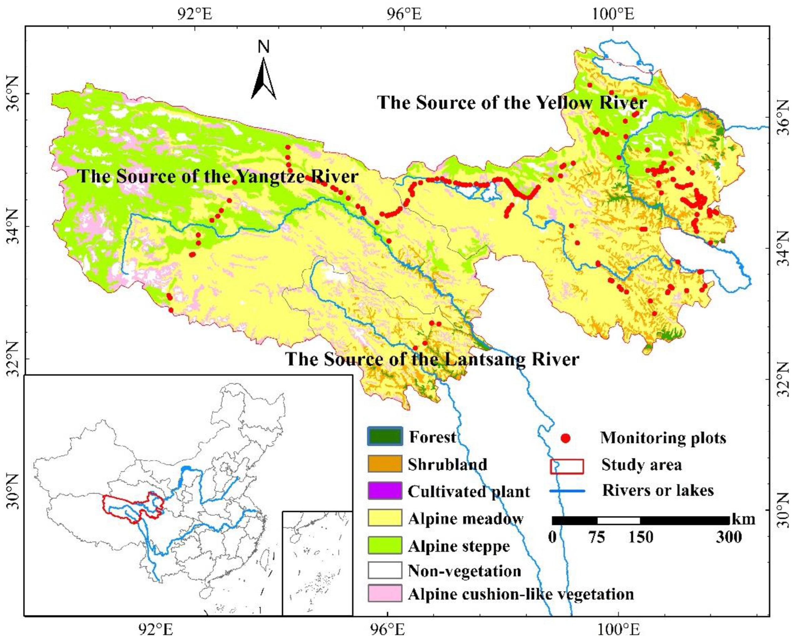
2.1. Study Area

TRSR, located in the northeast hinterland of Qinghai–Tibet Plateau (31°39′–36°16′N, 89°24′–102°23′E), is composed of the source area of the Yangtze River, Yellow River and Lantscang River, and it is known as the “Water Tower of China” (Figure 1). The topography of the TRSR is very rugged, mainly canyons and mountains, and there are permanent glaciers. The terrain is high in the northwest and low in the southeast, with an average altitude of about 4000 m. TRSR lies in a transitional zone between semi-arid and sub-humid climate conditions. Its climate is the typical plateau continental climate, which can be characterized by alternating cold and hot seasons and distinct dry and wet seasons [33]. The annual precipitation ranges from 262.2 to 772.8 mm, and the annual average temperature ranges from −5.38 to 4.14 °C [34]. The influence of East Asian summer monsoon is one of the reasons for the concentration of precipitation in summer [35]. Moreover, the annual sunshine duration ranges from 2312 to 2939 h, the average wind speed ranges from 1.1 to 4.3 m/s, and the relative humidity ranges from 49 to 66% [36]. The dominant vegetation type in this region is the alpine grassland (including alpine steppe and alpine meadow), which grows naturally in the harsh environment. Its growing season is very short, and summer is its most prosperous period. The alpine grassland in the TRSR has been steadily deteriorating over the past few decades as a result of interference from both natural and human influences, posing a serious risk to the water safety of those living downstream.

2.2. Data Source and Pre-Processing

The remote sensing products, including four FVC products (GEOV1 and GEOV2 at Copernicus Global Land Services, GLASS from Beijing Normal University, and MuSyQ from National Earth System Science Data Center) and the MODIS NDVI product from the Land Processes Distributed Active Archive Center website, utilized in this study were from 2001 to 2018. For the purpose of comparing the discrepancies between remote sensing products, we maintain the consistency of all remote sensing products in the coordinate system, temporal resolution and spatial resolution. The coordinate system of all remote sensing products was first uniformly changed into the WGS84 projection coordinate system by using the projection transformation tool. Then, via the bilinear interpolation method, the spatial resolution of the MuSyQ and GLASS FVC products was upscaled from 500 to 1000 m, and the spatial resolution of the MODIS NDVI was upscaled from 250 to 1000 m [37]. Finally, the MVC method was used to generate images with the maximum annual value from the remote sensing product image sets in July and August every year. The preprocessing of the remote sensing products mentioned above was performed in ArcGIS (v.10.2; ESRI, Redlands, CA, USA).

2.2.1. Remote Sensing Products

(a)
GEOV1 and GEOV2 FVC Products
The GEOV1 and GEOV2 were the officially part of the Copernicus Global Land Service (CGLS). The spatial and temporal resolutions of the GEOV1 and GEOV2 FVC products were 1 km and 10-days, respectively. The inversion algorithms of the GEOV1 and GEOV2 FVC products were neural networks in which the training data was CYCLOPE FVC data corrected using a scaling coefficient and the input data was provided by a SPOT-VEGETATION sensor (replaced with PROBA-VEGETATION sensor observations since 2014) [22,23,38]. Compared with the GEOV1 FVC products, the GEOV2 FVC products mainly improved the algorithm and combined with Savitzky–Golay filtering, time smoothing, application of meteorological data, and other key technologies to increase the spatio-temporal continuity of GEOV1 FVC. The GEOV1 and GEOV2 FVC data were stored in netCDF files, which were available at the CGLS website (https://land.copernicus.eu/global/products/fcover, accessed on 9 April 2021). The ArcGIS was used to extract the GEOV1 and GEOV2 FVC data from the netCDF files, and complete the FVC data reprojection and cropping.
(b)
GLASS FVC Product
The spatial and temporal resolutions of the GLASS FVC were 500 m and 8 days, respectively. Initially, the generalized regression neural network (GRNN) algorithm was utilized to produce the GLASS FVC. Since 2016, it has been replaced by the multiple adaptive regression spline (MARS) algorithm, which has higher estimates for efficiency and accuracy. MOD09A1 product, one of the MODIS series products which provided surface spectral reflectance of MODIS bands 1–7 with 500 m resolution, has further undergone spatiotemporal filtering to remove cloud pollution and other unfavorable observational factors. Then, the reprocessed MOD09A1 data were selected as the input data of the MARS algorithm and the training data were FVC samples inversion via high-quality Landsat TM/ETM+ reflectance data [2,19]. The GLASS FVC product is available from the National Earth System Science Data Center (http://www.geodata.cn/, accessed on 16 September 2021). The preprocessing of the GLASS FVC product, including image stitching and projection, was performed by MODIS Reprojection Tool. Then, the ArcGIS was used to crop the GLASS FVC data.
(c)
MuSyQ FVC Product
The MuSyQ FVC product provides FVC data with a spatial resolution of 500 m and a time step of 4 days. Based on the MuSyQ leaf area index (LAI) products and the MODIS clumping index (CI) products, the MuSyQ FVC data were calculated using gap probability theory [21]. The MuSyQ FVC data were stored in HDF5 files, which were available on the National Earth System Science Data Center website (http://www.geodata.cn/, accessed on 1 June 2022). A MuSyQ FVC data preprocessor was developed using the python programming language (version 3.9) for extraction and stitching of the MuSyQ FVC data. Then, the ArcGIS was used to complete the MuSyQ FVC data reprojection and cropping.
(d)
MODIS NDVI Product
MOD13Q1 was one of the MODIS series products. It provides vegetation product data with a spatial resolution of 250 m after 16 days of composite processing, mainly including NDVI data, enhanced vegetation index (EVI) data, and reflectance data of red, blue, near-infrared bands, etc. [39]. The MOD13Q1 product stored on the Land Processes Distributed Active Archive Center website (https://lpdaac.usgs.gov/, accessed on 19 September 2022) can be free to acquired. We extract the MODIS NDVI data from the MOD13Q1 product via MODIS Reprojection Tool. The preprocessing such as image stitching, reprojection, and cropping, was performed by this tool.

2.2.2. Meteorological Data

The temperature and precipitation data were provided by the European Centre for Medium-Range Weather Forecasts (ECMWF), named the fifth-generation ECMWF atmospheric reanalysis of the global climate (ERA5). ERA5 is part of the Copernicus Climate Change Service with a spatial resolution of 0.1° (about 10 km) [40]. Through the downscaling method developed by Jing et al. (2016), based on precipitation and surface characteristics, the spatial resolution of ERA5 was resampled to 1 km [41]. These temperature and precipitation data with spatio-temporal resolutions were 1 month and 1 km, respectively, which were downloaded from the National Earth System Science Data Center (http://www.geodata.cn/, accessed on 17 October 2022). In this study, the average temperature was calculated by averaging temperatures from June to August, and the accumulated precipitation was obtained by adding precipitation from June to August.

2.2.3. Auxiliary Data

The land cover map is a 1:1,000,000 spatial distribution map of vegetation types in China, which is derived from the Resources and Environmental Sciences and Data Center of the Chinese Academy of Sciences (https://www.resdc.cn/, accessed on 1 September 2022). It reflects the spatial distribution map of many vegetation types in China, such as meadow, steppe, coniferous forest, broadleaf forest, etc. It is the basic map of China’s national natural resources and physical geographical characteristics, and it comprises indispensable scientific data for the study of global eco-environmental change and monitoring.

2.2.4. Field Measured FVC Data

We delineated 243 remote sensing monitoring plots in the TRSR from July to August 2017, and each plot was 250 × 250 m in size [6] (Figure 1). At each remote sensing monitoring plot, we acquired high-resolution aerial images through aerial photography using unmanned aerial vehicles (UAV), named DJI Phantom 4 Professional Edition. The UAV can fly precisely and hover smoothly, since it uses the global positioning system/global navigation satellite system dual-satellite positioning module [5]. The spatial resolution of the aerial image obtained by an UAV flying at the relative altitude of 20 m is about 1 cm. We can clearly distinguish the vegetation pixels and non-vegetation pixels in these aerial images, so that we can obtain reliable vegetation coverage data. The specific field sampling plan and the process of obtaining measured FVC data from aerial images can be referred to in our previous studies [6,31,42].

2.3. Methods

2.3.1. Dynamic Monitoring Method of Alpine Grassland Cover

In this study, the Theil-Sen slope estimation method is used to estimate the spatial distribution trends of the alpine grassland in the TRSR, and the MK test method is used to test the significance of these trends. The Theil-Sen slope is the median value of the calculated long-time series and is commonly used to determine the magnitude of the rise and fall of the trend in long-time series data [43]. The MK test is a nonparametric statistical test used to determine the significance of the trend [44,45]. Both the methods are non-parametric statistical methods, which have a solid statistical theoretical basis and can effectively reduce the impact of missing values and outliers on long-time series data, widely used in vegetation, meteorology, hydrology, and ecological long-term time series trend analysis [46,47]. The formula of the Theil-Sen slope estimation method (Formula (1)) and MK test method (Formulas (2)–(5)) are as follows.
β = mean ( X b X a b a ) ( 2001 a < b 2018 )
S = b = 1 n 1 a = b + 1 n s g n ( X b X a )
s g n ( X b X a ) = ( 1 , X b X a > 0 0 , X b X a = 0 1 , X b X a < 0 )
s ( S ) = n ( n 1 ) ( 2 n + 5 ) 18
Z = ( ( S 1 ) / s ( S ) , S > 0 0 , S = 0 ( S + 1 ) / s ( S ) , S < 0 )
where Xa and Xb are the pixel value of remote sensing products in year a and year b. β < 0 denotes decreasing trend, and β > 0 denotes an increasing trend. n is the length of the period from year a and year b, α is the confidence levels, and Z is the standardized test statistic. Z1−α/2 is the value corresponding to the confidence level α. Confidence level α = 0.05 and α = 0.01 are used in this study, which correspond to Z1−α/2 values of 1.96 and 2.58, respectively. When |Z| > 1.96 and |Z| > 2.58, it indicates that the trend passes the significance test of 95% and 99%, respectively. Based on the β and Z values, this study divides the changing trend of all remote sensing products’ value into five levels (Table 1).

2.3.2. Influencing Factors of Dynamic Change of Alpine Grassland Cover Analysis Method

The partial correlation analysis method is one of the popular methods to research the influencing factors of vegetation dynamic change, since it can effectively exclude the influence of other variables and investigate the correlation between vegetation index and another variable, such as climate factors, human factors, etc. [8]. The values of partial correlation are between −1 and 1. The negative partial correlation coefficient means that factor 1 and factor 2 are negatively correlated when the third factor is controlled, while the positive partial correlation coefficient is the opposite, and 0 means that there is no phase relationship [48]. In this study, the partial correlation analysis method was used to quantitatively investigate the response of alpine grassland in the TRSR to average temperature when the cumulative precipitation factor was controlled. In addition, the response of alpine grassland in TRSR to accumulated precipitation was investigated when the average temperature factor was controlled [49]. The calculation formulas are as follows.
r x y = i = 1 n ( x i x ¯ ) ( y i y ¯ ) i = 1 n ( x i x ¯ ) 2 i = 1 n ( y i y ¯ ) 2
r x y , z = r x y r x z r y z ( 1 r x z 2 ) ( 1 r y z 2 )
where rxy represents the correlation coefficient between the variable x and variables y. xi and yi represent the value of the variable x and variables in year i. n represents the total number of years. rxy,z represents the partial correlation coefficient between variable x and variables y after controlling variable z. The p values are used to assess significance when p < 0.05 is considered significant at the confidence level of 95%.

2.3.3. Maximum Value Composite Method

The MVC method can obtain the maximum value of remote sensing image pixels in a period and can effectively remove the possible outliers in some remote sensing images [50]. The formula of the MVC method is as follows.
P i = m a x ( p 1 , p 2 , , p t )
where Pi is the maximum pixel value of remote sensing product in year i. p denotes that in year i, the value of a remote sensing product contains t images from July to August, and pt denotes the value of the t image.

2.3.4. Coefficient of Variation and Standard Deviation

In this study, the coefficient of variation (CV) and standard deviation (SD) are used to determine the stability and inter-annual fluctuations of the inter-annual variation trend of long-time series data [51]. The calculation formulas are as follows.
C V = S D A
S D = i = 1 n ( F i F ¯ ) n
where CV, SD, and A refer to the value of the coefficient of variation value, standard deviation value, and average value of the long-time series data, respectively. n is the length of the study period. F i and F ¯ represent the value in year i and the average value in study period, respectively.

2.3.5. Direct Validation Method and Accuracy Assessment

The direct validation method uses the measured FVC values to compare the FVC product pixel values [52,53]. Two statistical indicators are selected for accuracy validation, including coefficient of determination (R2) and root mean square error (RMSE), which are used to evaluate the goodness of fit and uncertainty, respectively [13]. R2 and RMSE were calculated as follows:
R 2 = 1 i = 1 N ( F i f i ) 2 i = 1 N ( F i f ¯ ) 2
R M S E = 1 N i = 1 N ( F i f i ) 2
where N is the number of the monitoring plots. F i and f i represent the measured FVC values and the values of FVC product pixel, respectively. f ¯ represents the average values of FVC product pixel.

3. Results

3.1. Spatio-Temporal Characteristics of Different Remote Sensing Products

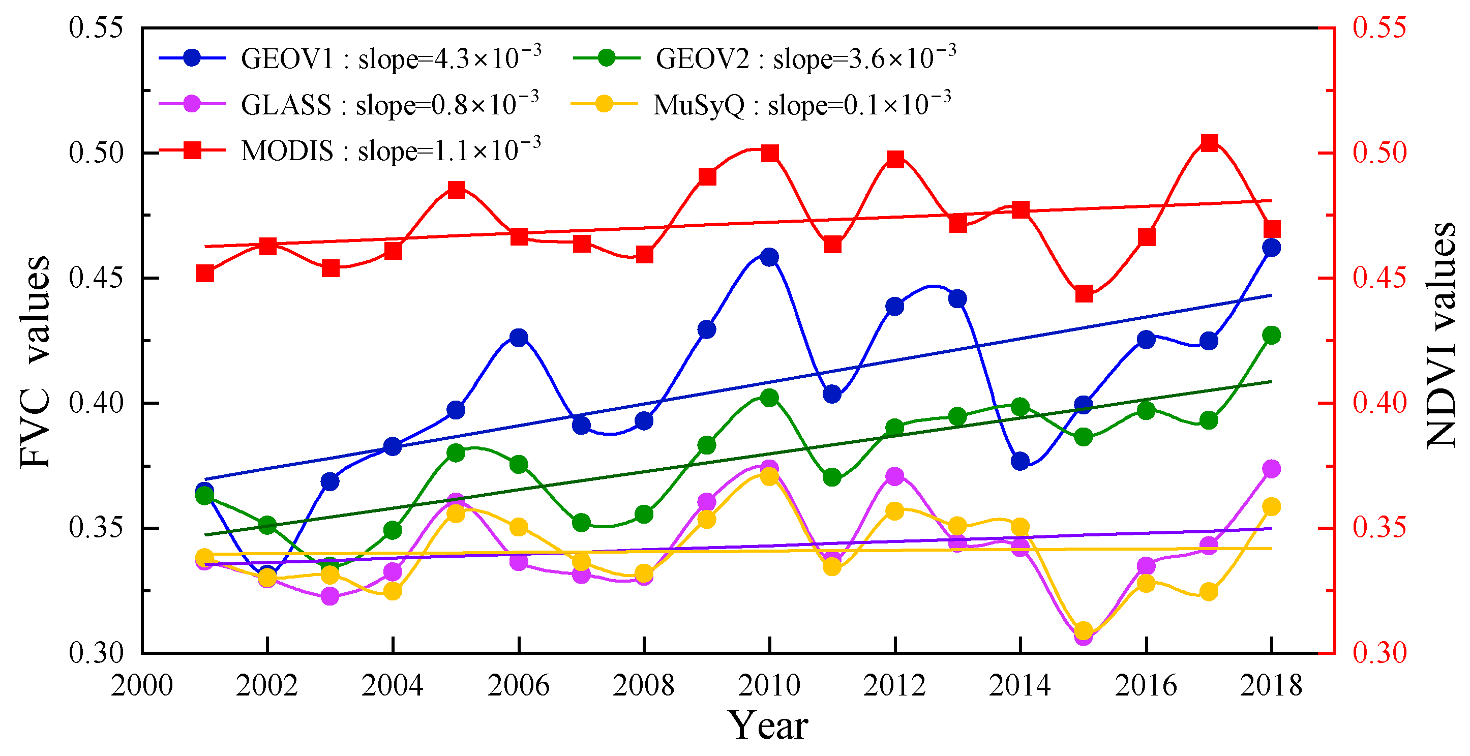
3.1.1. Consistency and Inconsistency of Temporal Changing Characteristics

The inter-annual variation trend of the average values of the MODIS NDVI and the FVC of the four FVC products all showed positive growth (slope > 0) (Figure 2). However, the changing trends of these five remote sensing products were noticeably different. The inter-annual growth rate of the average value of the MODIS NDVI was at a moderate level (1.1 × 10⁻³/a), which was significantly lower than the inter-annual growth rate of the average value of the GEOV1 FVC (4.3 × 10⁻³/a) and GEOV2 FVC (3.6 × 10⁻³/a). In addition, the inter-annual growth rate of the average value of the GLASS FVC (0.8 × 10⁻³/a) and MuSyQ FVC (0.1 × 10⁻³/a) increased relatively gradually (Table 2). The values of the coefficients of variation and standard deviation of the MODIS NDVI product, GLASS and MuSyQ FVC products were also relatively low, compared to those of the GEOV1 and GEOV2 FVC products.

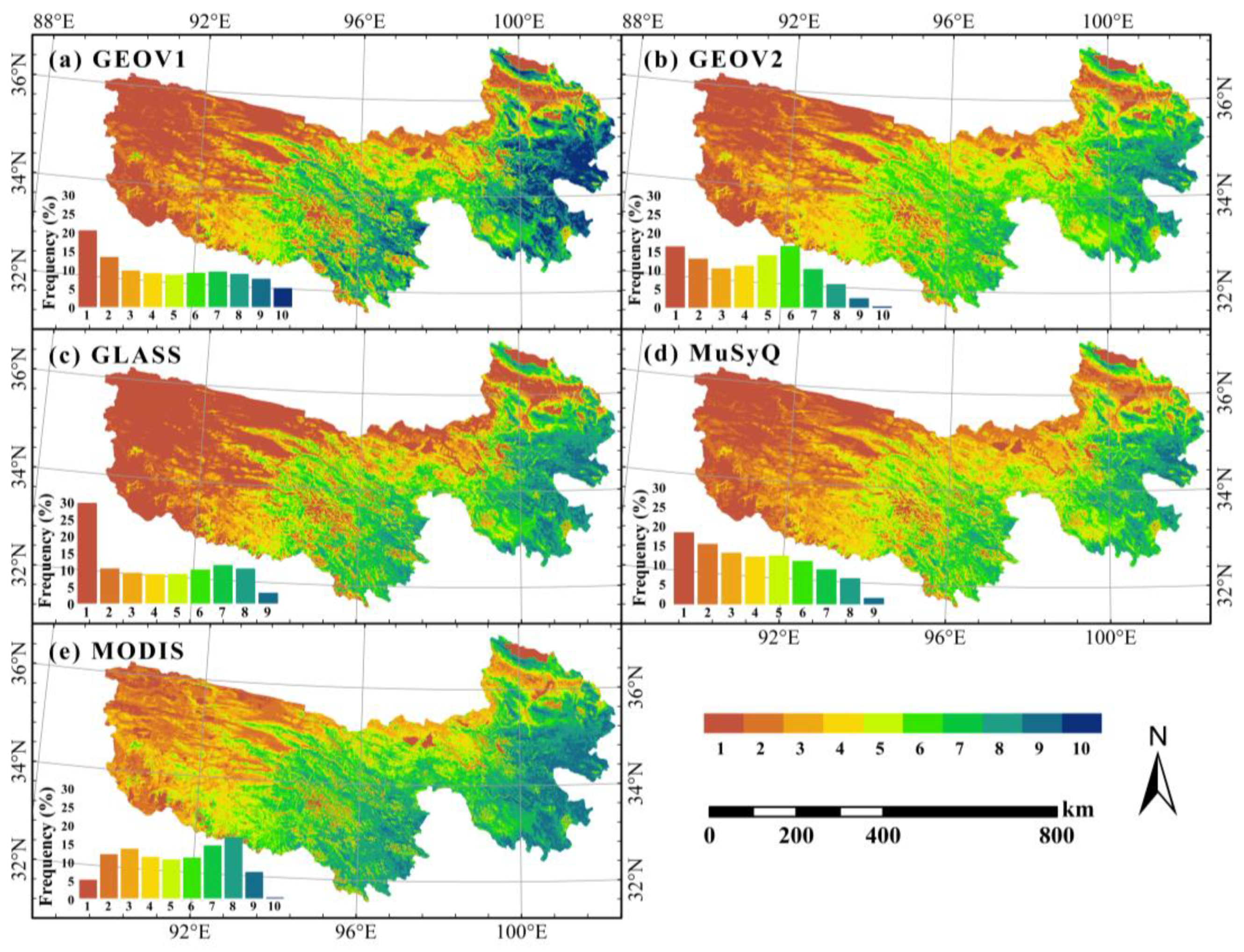
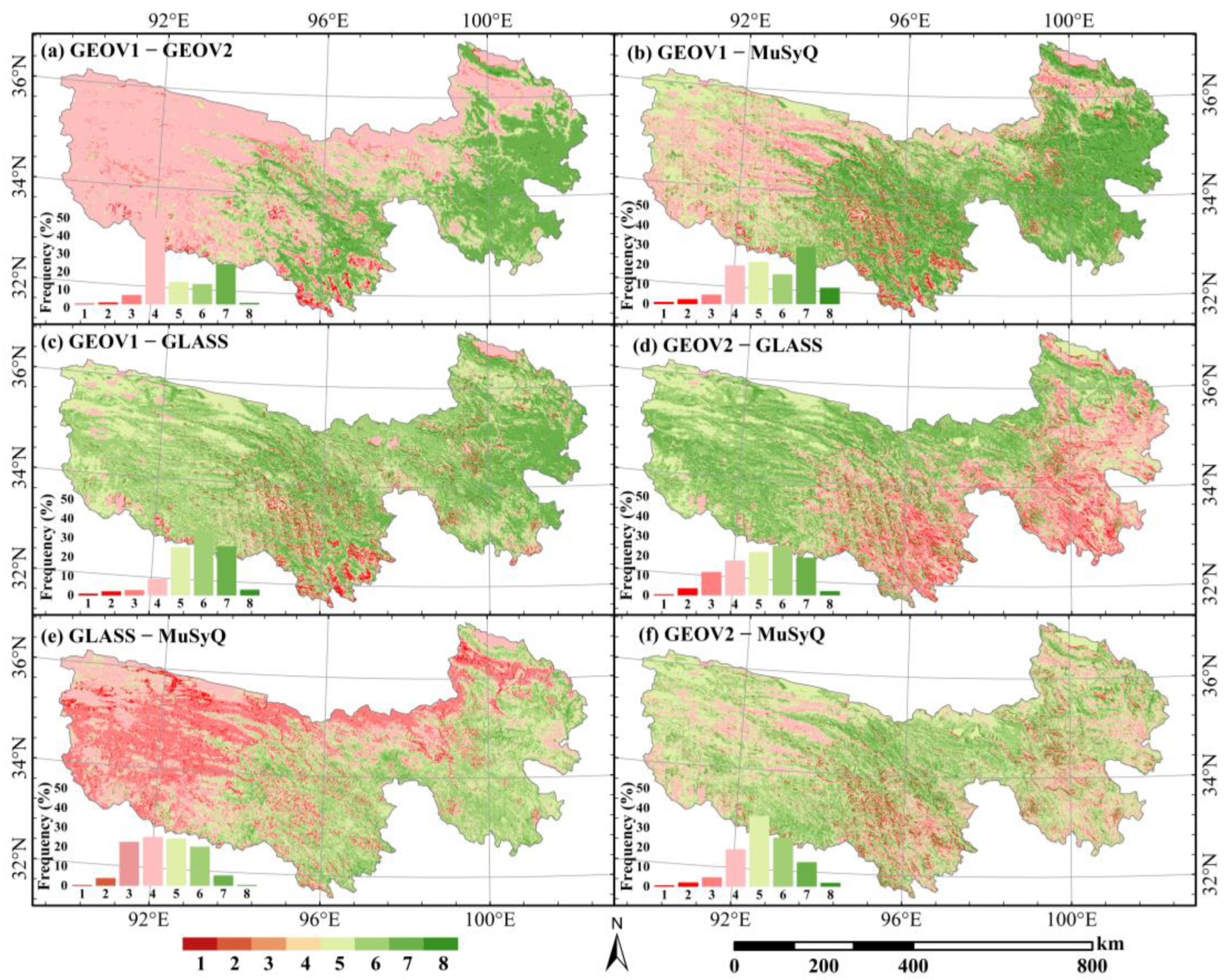
3.1.2. Consistency and Inconsistency of Spatial Distribution Characteristics

The spatial distribution pattern of the average values of the FVC of the four FVC products and the MODIS NDVI was relatively consistent, and the texture details were similar to the distribution pattern to a certain extent (Figure 3). On the whole, the southeastern, southern, and northern regions of the TRSR had quite high FVC values (or NDVI values), while the western and southern areas had relatively low FVC values (or NDVI values). In terms of the FVC values, the GEOV1 FVC products have the highest average FVC value (0.41), followed by the GEOV2 FVC product (0.38), the GLASS FVC product (0.34), and the MuSyQ FVC product (0.34). Moreover, the number of pixels among the four FVC products and the MODIS NDVI product at various FVC values (or NDVI values) intervals varies significantly (Figure 3). Particularly, the GEOV1 FVC product provided a large number of pixels with FVC values between 0.9 and 1.0, while the MODIS NDVI and the GEOV2, GLASS, and MuSyQ FVC data virtually never gave pixels with FVC values (or NDVI values) higher than 0.9. The pixel frequency of low FVC values (0 to 0.1) was around 10% higher in the GLASS FVC products than it was in the other three FVC products. The pixels with FVC values between 0.2 and 0.8 were more frequently provided by the GEOV2 and the MuSyQ FVC products.
The spatial distribution pattern of the difference images obtained by the pairwise difference of the four FVC products (GEOV1, GEOV2, GLASS, and MuSyQ) showed that the FVC values of the GEOV1 FVC product were slightly lower than that of the GEOV2 and MuSyQ FVC products in the north and west of the TRSR (most of the difference values were between −0.05 and 0) (Figure 4). However, the FVC values of the GEOV2 and MuSyQ FVC products were greater than those of the GEOV1 FVC product in the southern region of the TRSR, and the positive difference values were mostly between 0.1 and 0.2. Additionally, the difference values between the FVC values of the GEOV1 and GLASS FVC products were primarily positive, with the exception of a few regions southwest of the TRSR. The FVC values of the GEOV1 FVC product were greater than those of the GLASS product, and almost 75% of the positive difference values were higher than 0.05. The FVC values of GEOV2 FVC products in the western and northern regions of the TRSR were significantly higher than those of the GLASS and MuSyQ FVC products. However, the FVC values of the GEOV2 FVC product were significantly lower than the FVC values of the GLASS and MuSyQ FVC products in the south and southeast of the TRSR. Meanwhile, the FVC difference values between the GEOV2 and GLASS FVC products were higher than the FVC difference values between the GEOV2 and MuSyQ FVC products. For the FVC difference values between the GLASS and MuSyQ FVC products, the pixel frequency of positive difference was roughly equal to the pixel frequency of negative difference. The pixels of positive difference were primarily distributed in the south and southeast of the TRSR, whereas the pixels of negative difference were primarily distributed in the west and north of the TRSR.

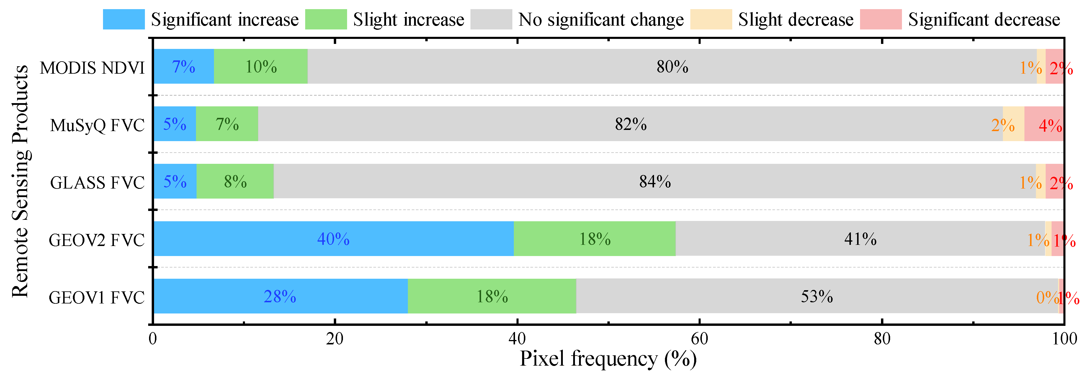
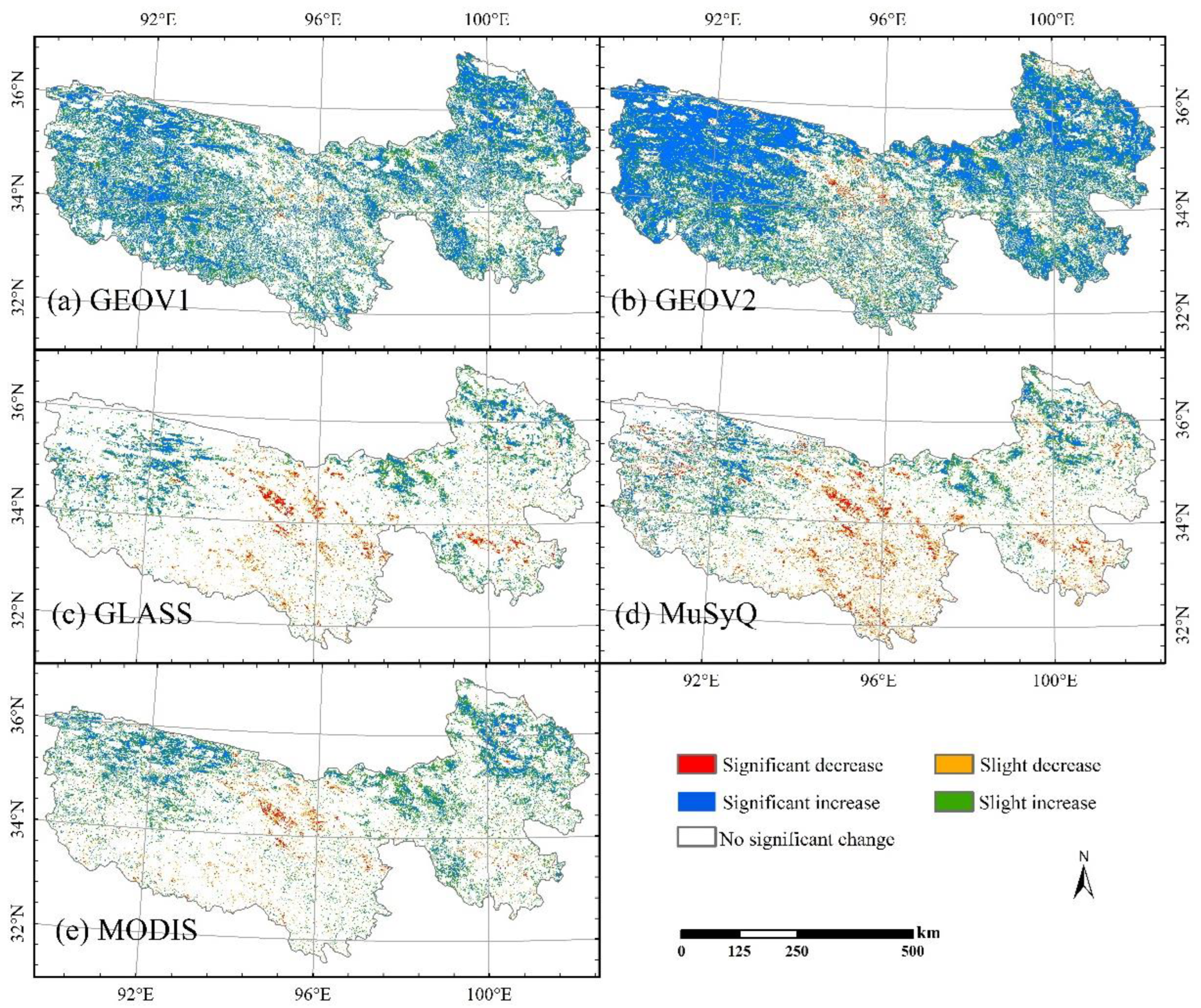
3.2. Consistency and Inconsistency of Alpine Grassland Changing Trend of Different Remote Sensing Products

The numerical diagram and the spatial distribution map of the trends of the four FVC products and the MODIS NDVI product over the last 18 years, obtained via the Theil-Sen slope estimation and Mann–Kendall test (Formulas (1)–(5)), showed that numerous pixels of the MODIS NDVI product, the GLASS FVC product, and the MuSyQ FVC product indicated no significant change trend (frequency more than 80%) (Figure 5 and Figure 6). Excluding the pixels with no significant changes, the pixel frequency in the five remote sensing products indicating a slight or significant increasing trend was much higher than that exhibiting a slight or significant decreasing trend. The pixel frequency of the GEOV1 and GEOV2 FVC products exhibited a considerably significant increasing trend, accounting for 27.99% and 39.63%, respectively, which was much higher than those of the MODIS NDVI product (6.73%) and the GLASS (4.83%) and MuSyQ (4.74%) FVC products. The pixel frequency showed a slight increasing trend that was the highest in the GEOV1 FVC product (18.47%), which was higher than those of the GEOV2 FVC product (17.73%), MODIS NDVI product (10.24%), GLASS FVC product (8.41%), and the MuSyQ FVC product (6.83%). Additionally, only a very small percentage of the pixels in the five remote sensing products, less than 5% overall, showed a significant or slight decreasing trend.
In the TRSR, according to the spatial distribution diagram integrating the changing trend of the four FVC products (Figure 7), there were three pixel categories with relatively high frequency: the first type comprised pixels in which the four FVC products all showed an insignificant change trend (26.9%), the second type comprised pixels in which two products exhibited an increasing trend (20.5%), and the last type comprised pixels in which only one product exhibited an increasing trend (18.4%). Less than 5% of the pixels were highly uncertain (one FVC product showed an increasing trend while another FVC product showed a decreasing trend), and less than 5% of the pixels were represented as a decreasing trend by multiple FVC products. Moreover, the TRSR’s center and southern regions contained the majority of the areas with a decreasing trend in FVC value, while the western and northeastern regions contained the majority of the areas with an increasing trend in FVC value.

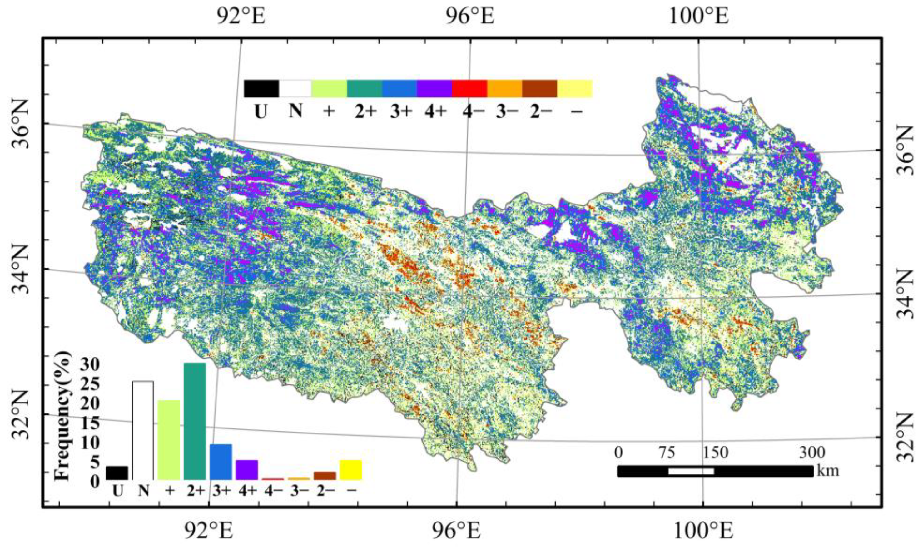
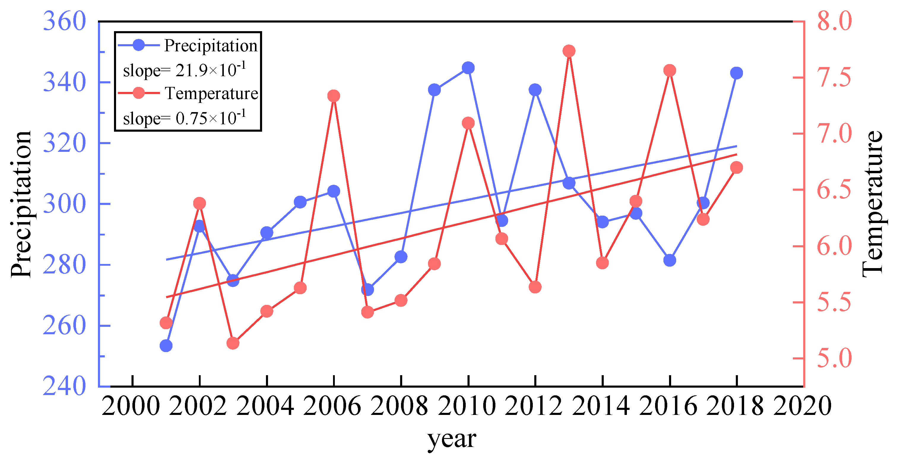
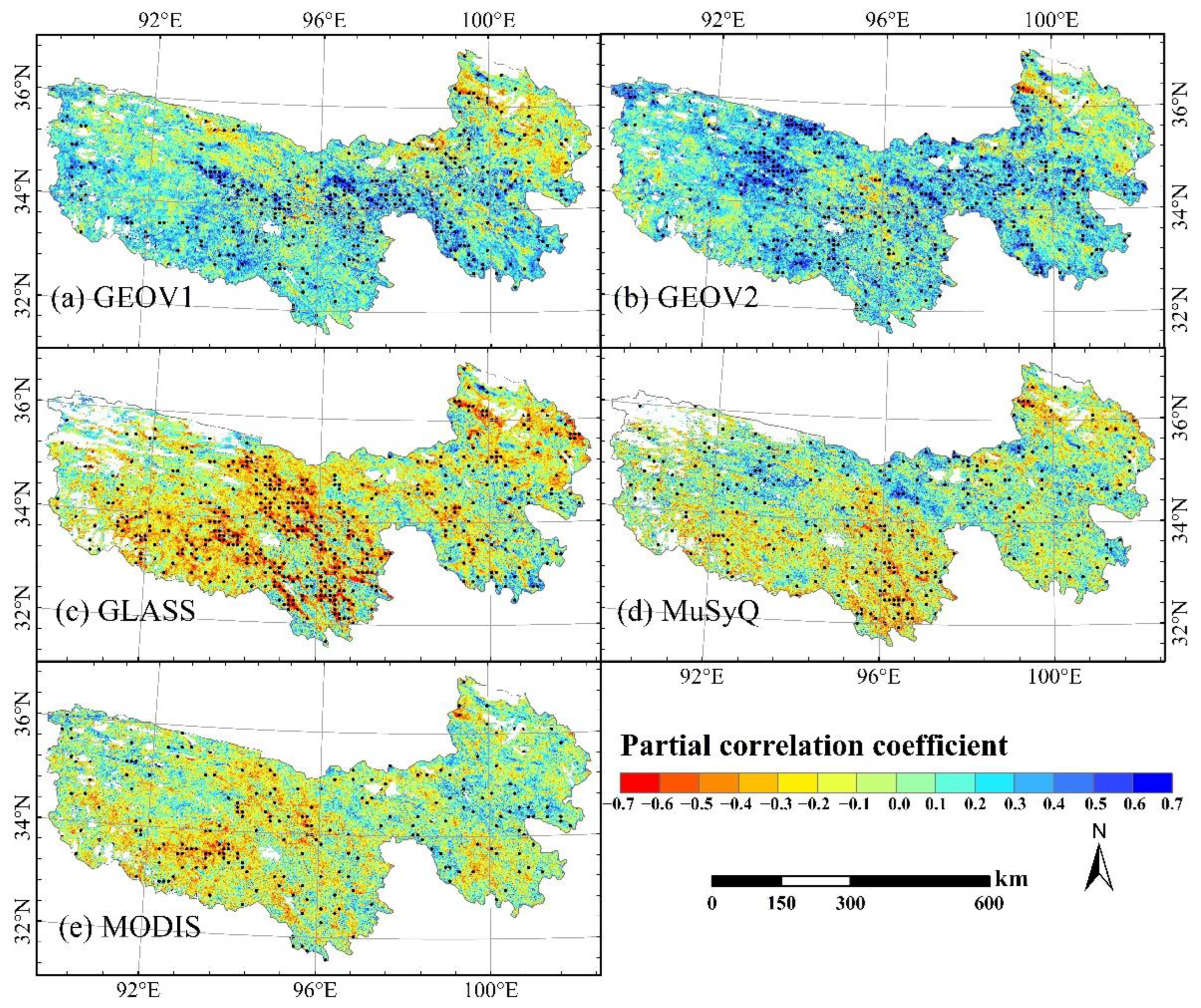
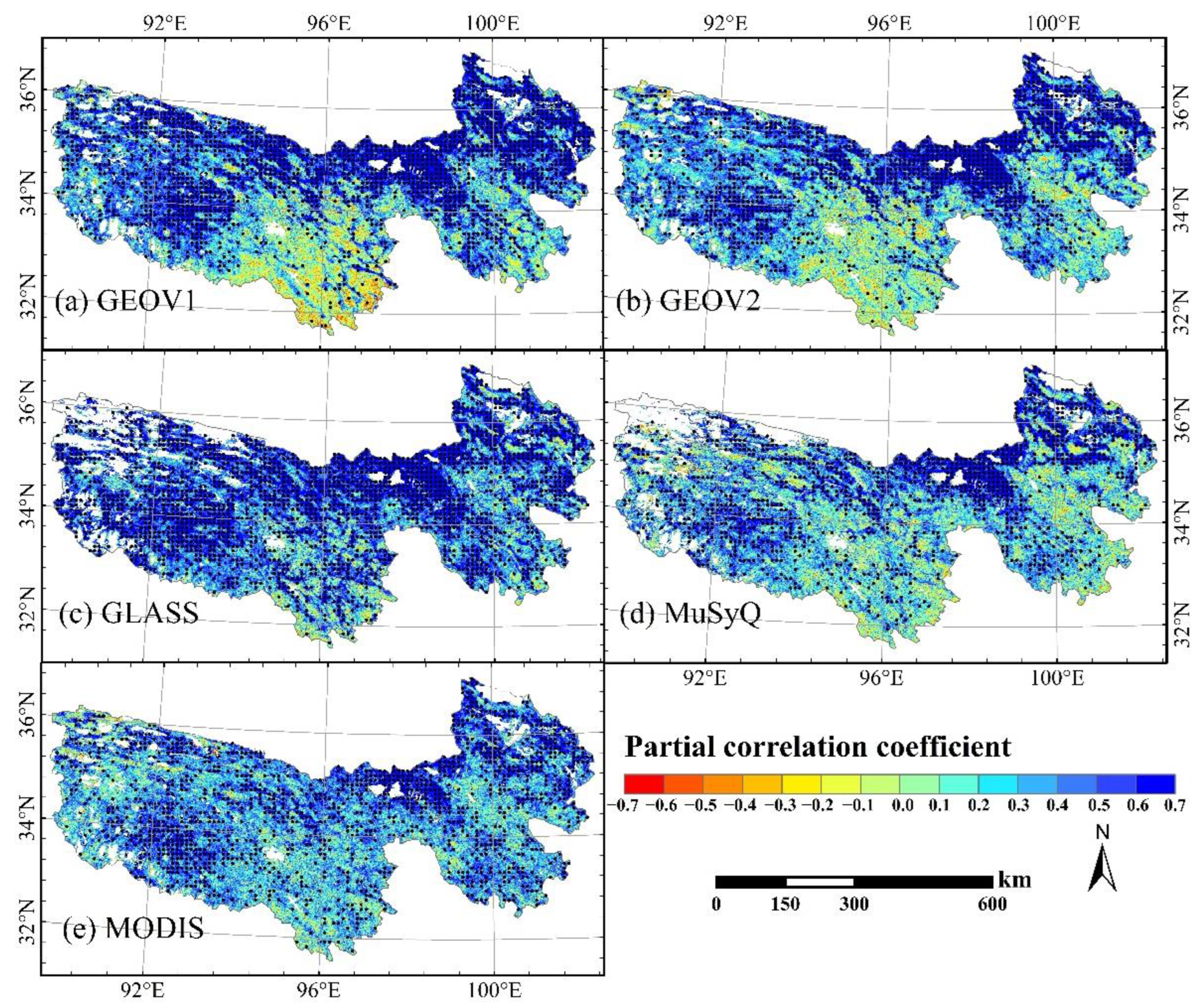
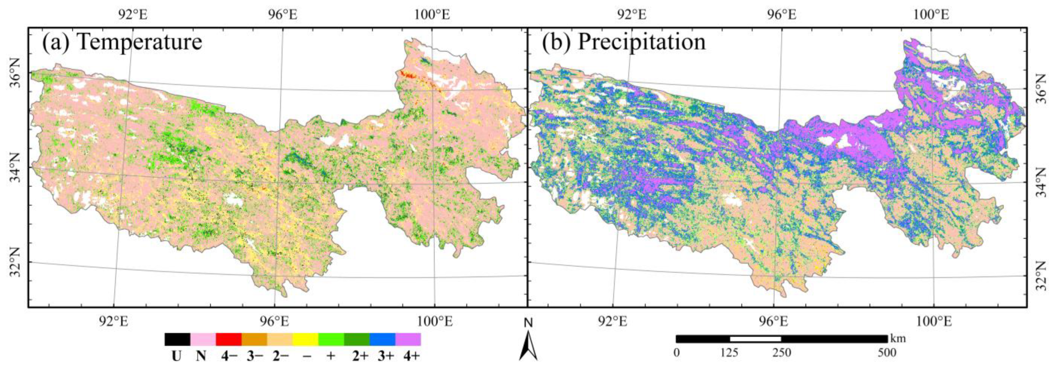
3.3. Consistency and Inconsistency of Factors Impacting Alpine Grassland Growth in Different Remote Sensing Products

From 2001 to 2018 in the TRSR, the cumulative summer precipitation increased at a rate of 2.19 mm/a, ranging from 250 to 350 mm, and the average temperatures ranged from 5.0 to 8.0 °C, increasing at a rate of 0.075 °C/a (Figure 8). Partial correlation coefficient spatial distribution maps of the five remote sensing products with average temperature and accumulated precipitation were obtained by partial correlation analysis method (Formulas (3) and (4)) (Figure 9 and Figure 10). The partial correlation coefficients between the values from the five remote sensing products and the average temperature values were varied in terms of numerical values and spatial distribution pattern (Figure 9). The pixels with the positive partial correlation coefficient in the GEOV1 and GEOV2 FVC products essentially covered the whole TRSR, while the pixels with the negative partial correlation coefficient were dispersed in the northeastern portion of the TRSR. More pixels with a negative partial correlation coefficient were found in the GLASS and MuSyQ FVC products, and these pixels were primarily located in the west and south of the TRSR. For the MODIS NDVI product, with a confidence level of 0.05, fewer pixels passed the significance test, and the absolute values of the partial correlation coefficient were obviously lower (the color of the pixels were lighter).
Strong consistency can be seen in partial correlation coefficients between data from the five remote sensing products and accumulated precipitation (Figure 10). The primary pixels in the TRSR were those with positive partial correlation coefficients, but there were certain discrepancies in their spatial distribution pattern. The whole TRSR was essentially covered by the pixels with the positive partial correlation coefficient in the GLASS FVC products, and the pixel value was high. In the MODIS NDVI product and the MuSyQ FVC product, the pixel value of the positive partial correlation coefficient was relatively small. The pixel partial correlation coefficient in the southern portion of the TRST was negative in the GEOV1 and GEOV2 FVC products.
With the significance test of 0.05 confidence level, the partial correlation coefficients between the values of the four FVC products and the average temperature and accumulated precipitation are integrated in Figure 11. The spatial distribution of integrated partial correlation coefficients (Figure 11a) showed that the pixels with no significant relationship between the four FVC products and the average temperature accounted for the highest proportion (69.9%), which was higher than the pixel proportion with one FVC product showing a significant correlation (23.1%) (Table 3). The proportion of the pixels that showed a significant correlation via two or more FVC products was relatively scarce (less than 8%), and these pixels were mainly distributed in the center part of the TRSR. On the contrary, there was only a small proportion of the pixels (29.7%) that showed no significant correlation between the four FVC products and the accumulation of precipitation. In addition, the proportion of the pixels, which showed a significant positive correlation via the three FVC products and four FVC products, was relatively high (30.7%), and these pixels were primarily centered in the northern part of the TRSR. The proportion of the pixels that showed a significant positive correlation via the one FVC product and two FVC products was the highest (37.8%), and these pixels were primarily clustered in the western part of the TRSR (Figure 11b and Table 3).

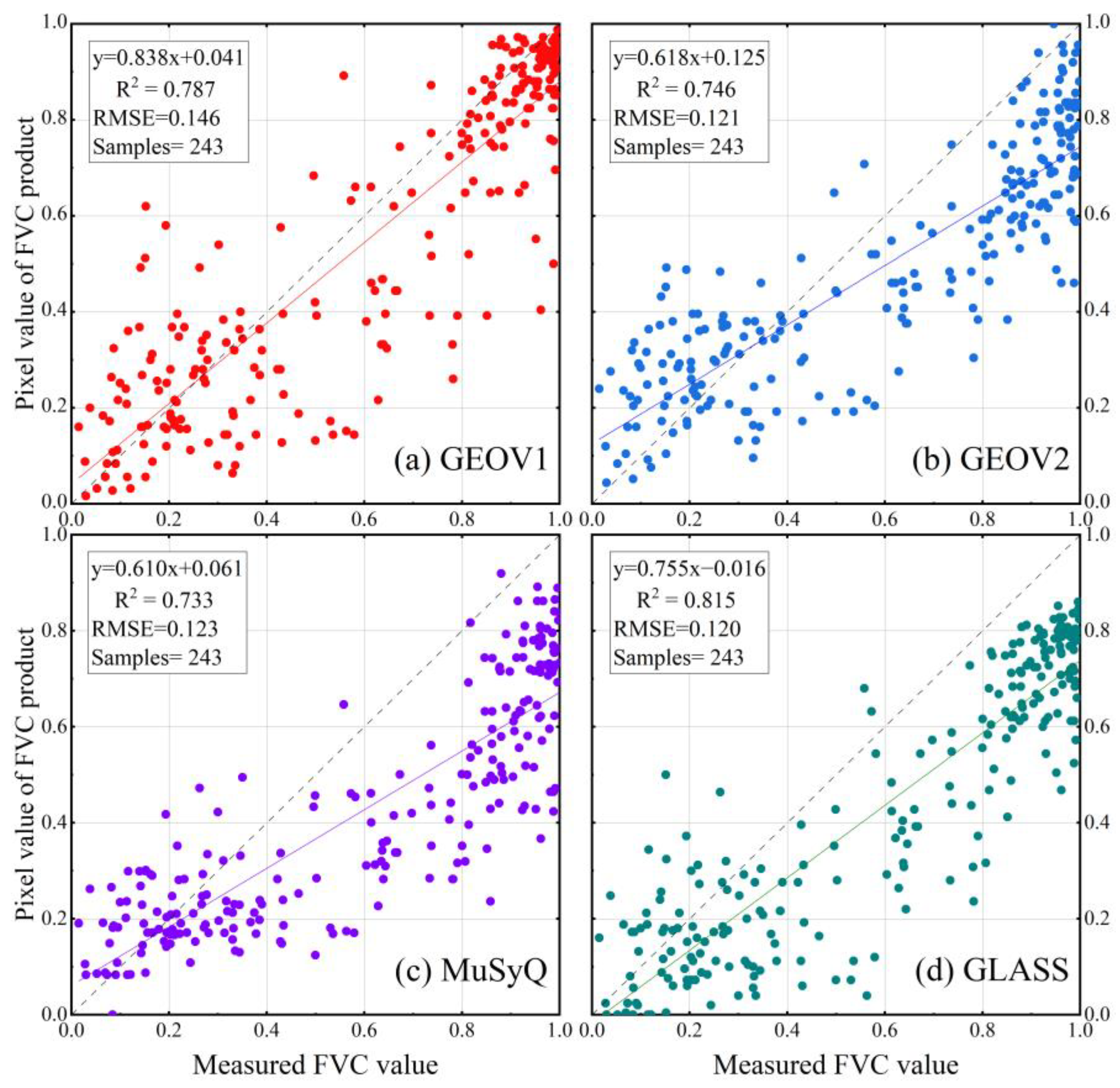
3.4. Validation of the FVC Products in the Alpine Grassland Ecosystem

Based on the measured FVC values of monitoring plots in the TRSR, the direct validation results of FVC products showed that these FVC products had good accuracies (Figure 12). The GLASS FVC products had better accuracy assessment indexes than other FVC products (R2 = 0.815, RMSE = 0.120). The accuracy assessment indexes of the GEOV1 FVC product (R2 = 0.787, RMSE = 0.146) were close to that of the GEOV2 (R2 = 0.746, RMSE = 0.121) and MuSyQ (R2 = 0.733, RMSE = 0.123) FVC products. However, for the GEOV2, GLASS, and MuSyQ FVC products, the scatter of the points composed of measured FVC values and pixel values of the corresponding FVC product were located below the 1:1 contour line, showing an underestimation phenomenon. For the GEOV1 FVC products, more scattered points were clustered around the 1:1 contour line, but they were relatively scattered.

4. Discussion

4.1. Spatio-Temporal Discrepancies of Different Remote Sensing Products

Monitoring the ecological environment via remote sensing technology has attracted increasing attention, but the inconsistency of remote sensing products will affect how the ecological environment is assessed and how its effects are understood [30,54,55]. Our research results showed that although the yearly average value differences between the four FVC products were between 0.02 and 0.06, the inter-annual change rates of the average values of the four FVC products were highly discrepancy. In comparison to the GLASS FVC product (0.8 × 10⁻³/a) and MuSyQ FVC product (0.1 × 10⁻³/a), the inter-annual change rates of the average value of the GEOV1 FVC product (4.3 × 10⁻³/a) and GEOV2 FVC product (3.6 × 10⁻³/a) were much faster. One of the crucial statistical indicators to assess regional vegetation change is the rate of inter-annual vegetation change. Varied remote sensing products, however, produce different information about vegetation change as a result of these FVC products cannot provide the same FVC values. These “unreal” or “uncertain” facts about vegetation changing trend would deceive the relevant departments while drafting environmental protection policies, compromising the ecological security and stability of the region. We quantified the spatial distribution pattern of the FVC products and performed spatial difference processing on the spatial distribution pattern of the four FVC products in order to more thoroughly analyze the effects of differences among the various FVC products on the monitoring results of alpine grassland change.
Our results demonstrate that there were clear disparities in the spatial distribution of the four FVC products and that the FVC value of the GEOV1 product was systematically larger than that of the GLASS FVC product. Where there is sparse alpine grassland (mostly alpine steppe) in the northwest of the TRSR and dense alpine grassland (primarily alpine meadow) in the southeast of the TRSR, the differences were primarily focused (Figure 7). The cause may be that various algorithms and training data of different FVC products lead to different estimation accuracies of FVC values of diverse biological communities by the FVC product inversion models [6,25,56]. Additionally, the quality of the input data and the quality of the surface reflectance captured by sensors, had a great impact on how accurate the FVC value estimations were. The moderate spatial resolution of the SPOT-VEGETATION, PROBA-VEGETATION, and MODIS sensors (>250 m) was an important factor [9,57,58]. The surface reflectance captured by these sensors in the highly heterogeneous underlying surface of the TRSR was a mixed information reflection, which contains diverse biological community types (or different land use types) [59,60,61,62]. Moreover, because of the high altitude and rugged terrain in the TRSR, the bidirectional reflection distribution function (BRDF) was even more complex [17,63,64,65]. As a result, the surface reflectance information obtained by different sensors may differ significantly. Thus, it may provide highly ambiguous study results to analyze environmental change via only the long-time series of a single remote sensing product. It is vital to conduct an authenticity validation on remote sensing products to ascertain whether their quality is within the expected range before conducting further study on environmental change. This activity is essential to ensuring valid research results [37,59,66].

4.2. Analysis of Alpine Grassland Change Trends of Different Remote Sensing Products

The alpine grassland change trend in the TRSR from 2001 to 2018 was largely unnoticeable, with some alpine grassland even improving, but still, a little alpine grassland degraded according to the demonstration via the five remote sensing products used in this study (Figure 5 and Figure 6), which was consistent with the results of other scholars [30,67,68]. However, the spatial distribution pattern and statistics values of the alpine grassland change trend in the TRSR simulated by the five remote sensing products were noticeably discrepant (Figure 5 and Figure 6). In the TRSR, as compared to the alpine grassland change trend simulated by the MODIS NDVI product, more alpine grassland deterioration occurred in the southern region, and less alpine grassland improvement happened in the northeast based on the MuSyQ and GLASS FVC products (Figure 6). The fact that both the GLASS and MuSyQ FVC products originated from MODIS reflectance data may explain why the overall discrepancy was not the same as the GEOV1 and GEOV2 FVC products [2,19,21]. Based on the GEOV1 and GEOV2 FVC products, it was determined that the alpine grassland was obviously improved, especially in the southeast and west of the TRSR (Figure 6). Figure 5 also shows that the proportion of pixels with a greening trend found utilizing the GEOV1 and GEOV2 FVC products was significantly higher than that found using the MODIS NDVI product and the MuSyQ and GLASS FVC products. We further integrated, categorized, and quantified the changing trend of FVC values of the four FVC products in order to better analyze the effects of different remote sensing data sources on the monitoring results of alpine grassland change (Figure 7). We found that the pixels with an uncertainty of alpine grassland changing trend in the TRSR can be divided into three categories. The first category, which made up just a very small part (5%), was a highly uncertain pixel category, which was a pixel with an opposing alpine grassland change trend acquired from the distinct FVC products. The second category was the pixel category with uncertainty to a certain extent, which was composed of a significant portion (roughly 50%) and refers to the pixel with one or two types of FVC products showing a trend of improvement (or deterioration). These pixels may be the different pixels between the remote sensing products produced from the different data sources or the remote sensing products produced from the same data source (such as the GEOV1 and GEOV2 FVC products). Finally, the third category, which constituted a relatively tiny part (15%), was a minor uncertain pixel category, since at least three remote sensing products demonstrate that the alpine grassland in this area had a tendency to improve (or deterioration). The variance in vegetation change trends among the various remote sensing products can be attributed to two key factors. First, there were certain discrepancies, the data of various remote sensing satellites and measured data (or the reference truth data) were utilized in the inversion of different remote sensing products [7,58,69]. Additionally, there were discrepancies among the sensors and the temporal and spatial resolution of various remote sensing satellites. Remote sensing products will be impacted by all of these aspects [60]. Another uncertainty of FVC products resulted from the uncertainty of remote sensing parameter inversion theory, including the performance and transfer of the machine learning arithmetic, the ill-posed inversion problem, etc. [6,56]. Our study demonstrated that one remote sensing product replaced by another remote sensing product may not yield similar results. While the ground-measured data were absent, cross-validation between remote products or research on the trend of vegetation change using various remote sensing products is required for the purpose of assessing the relative reliability of the research results [59,70,71]. It is an effective way to lessen the uncertainty in the study of vegetation change caused by the inconsistency of remote sensing products [68], but it is urgent to produce a collection of remote sensing products that possesses adequate representation and qualification and can be served as a calibration or benchmark for research on vegetation change and other relevant topics.

4.3. Assessment of the Uncertainty of the Direct Validation Results of the FVC Products

Filed measurement data are an essential prerequisite for us to understand the quality of remote sensing products. Although some scientific research teams have used some global validation sites to validate the overall accuracy of these FVC products, there are still many regions, such as the Qinghai–Tibetan Plateau (QTP), where the accuracy of these FVC products is not available. Based on measured FVC data in the TRSR on the QTP, our direct validation results showed that, from an annual maximum perspective, the four FVC products all had a certain underestimation in the medium-high vegetation cover area, which may be related to the limited measured data of the FVC production scientific research team on the QTP [37]. However, in this study, our validation results may be affected by the mismatch between the ground measurement range and the pixel scale of the FVC products since each monitoring plot measures approximately an extent of 250 × 250 m, which is much smaller than a pixel of the FVC products (1 × 1 km). Affected by the heterogeneity of the underlying surface of the monitoring plots, the spatial representation ability of some monitoring plots may be insufficient, which may introduce certain uncertainties into the validation of the FVC products [52,60]. Additionally, we used one year’s data to validate these FVC products, but the validation of FVC products requires long-term work, as eco-environment monitoring is also long-term work. Therefore, on the QTP, both the quality of these FVC products and the validation strategy of FVC products have great room for improvement. This also further emphasizes that the application groups of remote sensing products should pay more attention to the fitness of remote sensing products in the region scale because the quality of remote sensing products will affect the accuracy of the eco-environment monitoring and simulation research results.

4.4. Analysis of the Factors Impacting Alpine Grassland Growth of Different Remote Sensing Products

Climate is a key natural factor affecting the growth of alpine grassland. The change in the climate and environmental conditions will affect the growth of alpine grassland [72]. Our results show that from 2001 to 2018, the average temperature and cumulative precipitation have gradually increased, and the alpine grassland in the TRSR has been developing well [28,73]. This was similar to the conclusion of previous studies, i.e., the warm and humid total environment has prolonged the growing season of alpine grassland in the alpine ecosystem and has promoted the alpine grassland growth to be promising and prosperous (Figure 8) [29,54,74]. However, there was still some discrepancy in the factors that influence alpine grassland growth change in the TRSR. Differences in research methods, time span, and geographical location were the main reasons for the inconsistent results, which has reached a consensus. Nevertheless, according to our research, we also found that different remote sensing products would produce diverse research results when used to examine the factors influencing alpine grassland growth (Figure 9 and Figure 10). For example, at the confidence level of 0.05, the spatial distribution pattern of the partial correlation coefficient between alpine grassland and the accumulated precipitation in the TRSR simulated by the four FVC products was significantly different, and the discrepancy of the spatial distribution pattern of the partial correlation coefficient between alpine grassland and the average temperature was more significant. Three or more FVC products revealed that the number of pixels that were significantly correlated with the accumulated precipitation in TRSR was relatively large (about 30%) and primarily distributed in the northern region of the TRSR, while two or more FVC products revealed that the number of pixels that were significantly correlated with average temperature was very small (less than 6%). This demonstrated that accumulated precipitation had a significant impact on alpine grassland growth in the TRSR (Figure 11). However, around 70% and 32% of the pixels, respectively, demonstrated that the alpine grassland was insensitive to the average temperature and accumulated precipitation. In addition, the average temperature and accumulated precipitation influenced alpine grassland in the TRSR, as shown by the fact that only one or two FVC products were present in around 28 and 40 percent of the pixels, respectively (Table 3). Our research showed that the study of the influencing factors of alpine grassland growth change will be uncertain due to the uncertainty of remote sensing products. Therefore, it is essential to conduct authenticity validation on the remote sensing products utilized when assessing the driving mechanism of ecological environment change to better understand the constraints on alpine grassland growth.

5. Conclusions

The spatio-temporal changes of alpine grassland in the TRSR from 2001 to 2018 were analyzed in this study, based on the four international mainstream FVC products (including GEOV1, GEOV2, GLASS, MuSyQ) and MODIS NDVI product, via the Theil-Sen median slope trend analysis and Mann–Kendall significance test methods. In addition, by combining the temperature and precipitation data, the response of alpine grassland to meteorological factors was evaluated. Our results showed that the uncertainty of remote sensing products leads to significant discrepancies in the study conclusions such as the dynamic cover changes in alpine grassland. These discrepancies were not only reflected in the inter-annual growth rate of alpine grassland change, but also in the spatial distribution pattern in alpine grassland dynamic change. Meanwhile, the alpine grassland growth limits or driving factors that can be explained by each product were significantly different. Our study quantified the potential impact of remote sensing product differences or their own uncertainties on subsequent ecological environment monitoring and simulation studies. In the future, the accuracy of remote sensing products should be first validated before using them for eco-environmental monitoring or simulation studies at a regional scale. In addition, a reliable and highly accurate FVC dataset that plays a role in calibration at the regional scale should also be produced, which can effectively provide regional accuracy standards for the global FVC products and provide guidance for inversion algorithm optimization and mechanism model development of the global FVC products, improving the applicability of the FVC products.

Author Contributions

Conceptualization, R.H. and J.C.; methodology, R.H. and J.C.; validation, R.H. and J.C.; formal analysis, R.H. and J.C.; resources, R.H., J.C., Z.F. and Y.Y.; software, Z.F. and Y.Y.; writing—original draft preparation, R.H.; writing—review and editing, R.H. and J.C.; visualization, R.H. and J.C.; supervision, H.Y. and X.H.; funding acquisition, J.C., H.Y. and X.H. All authors have read and agreed to the published version of the manuscript.

Funding

This study was supported by grants from Guangxi Science and Technology Base and Talent Project (GuikeAD19245032), the National Natural Science Foundation of China (41801030, 41861016), Guangxi Key Laboratory of Spatial Information and Geomatics (19-050-11-22), and the Research Foundation of Guilin University of Technology (GUTQDJJ2017069).

Data Availability Statement

Not applicable.

Acknowledgments

Acknowledgement for the data support from “National Earth System Science Data Center, National Science & Technology Infrastructure of China (http://www.geodata.cn, accessed on 1 June 2022)”, “Beijing Normal University (http://glass-product.bnu.edu.cn/index.html, accessed on 16 September 2021)”, and “Copernicus Global Land Service Center (https://land.copernicus.eu, accessed on 22 April 2021)”.

Conflicts of Interest

The authors declare no conflict of interest.

References

  1. Jia, K.; Liang, S.; Gu, X.; Baret, F.; Wei, X.; Wang, X.; Yao, Y.; Yang, L.; Li, Y. Fractional Vegetation Cover Estimation Algorithm for Chinese GF-1 Wide Field View Data. Remote Sens. Environ. 2016, 177, 184–191. [Google Scholar] [CrossRef]
  2. Jia, K.; Liang, S.; Wei, X.; Yao, Y.; Yang, L.; Zhang, X.; Liu, D. Validation of Global Land Surface Satellite (GLASS) Fractional Vegetation Cover Product from MODIS Data in an Agricultural Region. Remote Sens. Lett. 2018, 9, 847–856. [Google Scholar] [CrossRef]
  3. Pörtner, H.-O.; Roberts, D.C.; Tignor, M.; Poloczanska, E.S.; Mintenbeck, K.; Alegría, A.; Craig, M.; Langsdorf, S.; Löschke, S.; Möller, V.; et al. (Eds.) Climate Change 2022: Impacts, Adaptation and Vulnerability. Contribution of Working Group II to the Sixth Assessment Report of the Intergovernmental Panel on Climate Change; Cambridge University Press: Cambridge, UK; New York, NY, USA, 2022; p. 3056. [Google Scholar] [CrossRef]
  4. Zhu, Z.; Piao, S.; Myneni, R.B.; Huang, M.; Zeng, Z.; Canadell, J.G.; Ciais, P.; Sitch, S.; Friedlingstein, P.; Arneth, A.; et al. Greening of the Earth and Its Drivers. Nat. Clim. Chang. 2016, 6, 791–795. [Google Scholar] [CrossRef]
  5. Chen, J.; Chen, Z.; Huang, R.; You, H.; Han, X.; Yue, T.; Zhou, G. The Effects of Spatial Resolution and Resampling on the Classification Accuracy of Wetland Vegetation Species and Ground Objects: A Study Based on High Spatial Resolution UAV Images. Drones 2023, 7, 61. [Google Scholar] [CrossRef]
  6. Chen, J.; Huang, R.; Yang, Y.; Feng, Z.; You, H.; Han, X.; Yi, S.; Qin, Y.; Wang, Z.; Zhou, G. Multi-Scale Validation and Uncertainty Analysis of GEOV3 and MuSyQ FVC Products: A Case Study of an Alpine Grassland Ecosystem. Remote Sens. 2022, 14, 5800. [Google Scholar] [CrossRef]
  7. Lin, X.; Chen, J.; Lou, P.; Yi, S.; Zhou, G.; You, H.; Han, X. Quantification of Alpine Grassland Fractional Vegetation Cover Retrieval Uncertainty Based on Multiscale Remote Sensing Data. IEEE Geosci. Remote Sens. Lett. 2021, 19, 2501705. [Google Scholar] [CrossRef]
  8. Feng, Z.; Chen, J.; Huang, R.; Yang, Y.; You, H.; Han, X. Spatial and Temporal Variation in Alpine Vegetation Phenology and Its Response to Climatic and Topographic Factors on the Qinghai–Tibet Plateau. Sustainability 2022, 14, 12802. [Google Scholar] [CrossRef]
  9. Liu, Y.; Li, Z.; Chen, Y.; Li, Y.; Li, H.; Xia, Q.; Kayumba, P.M. Evaluation of Consistency among Three NDVI Products Applied to High Mountain Asia in 2000–2015. Remote Sens. Environ. 2022, 269, 112821. [Google Scholar] [CrossRef]
  10. Montandon, L.M.; Small, E.E. The Impact of Soil Reflectance on the Quantification of the Green Vegetation Fraction from NDVI. Remote Sens. Environ. 2008, 112, 1835–1845. [Google Scholar] [CrossRef]
  11. Gao, X.; Huete, A.R.; Ni, W.; Miura, T. Optical-Biophysical Relationships of Vegetation Spectra without Background Contamination. Remote Sens. Environ. 2000, 74, 609–620. [Google Scholar] [CrossRef]
  12. Pattison, R.R.; Jorgenson, J.C.; Raynolds, M.K.; Welker, J.M. Trends in NDVI and Tundra Community Composition in the Arctic of NE Alaska Between 1984 and 2009. Ecosystems 2015, 18, 707–719. [Google Scholar] [CrossRef]
  13. Lin, X.; Chen, J.; Lou, P.; Yi, S.; Qin, Y.; You, H.; Han, X. Improving the Estimation of Alpine Grassland Fractional Vegetation Cover Using Optimized Algorithms and Multi-Dimensional Features. Plant Methods 2021, 17, 96. [Google Scholar] [CrossRef] [PubMed]
  14. Yang, J.; Chen, H.; Borjigin, N.; Zhao, M.; Zhou, Y.; Huang, Y. Validation of the MODIS LAI Product in Qinghai Lake Basin Combined with Field Measurements Using Landsat 8 OLI Data. Acta Ecol. Sin. 2017, 37, 322–331. [Google Scholar] [CrossRef]
  15. Gitelson, A.A.; Kaufman, Y.J.; Stark, R.; Rundquist, D. Novel Algorithms for Remote Estimation of Vegetation Fraction. Remote Sens. Environ. 2002, 80, 76–87. [Google Scholar] [CrossRef] [Green Version]
  16. Huang, S.; Tang, L.; Hupy, J.P.; Wang, Y.; Shao, G. A Commentary Review on the Use of Normalized Difference Vegetation Index (NDVI) in the Era of Popular Remote Sensing. J. For. Res. 2021, 32, 1–6. [Google Scholar] [CrossRef]
  17. Chen, J.; Yi, S.; Qin, Y. The Contribution of Plateau Pika Disturbance and Erosion on Patchy Alpine Grassland Soil on the Qinghai-Tibetan Plateau: Implications for Grassland Restoration. Geoderma 2017, 297, 1–9. [Google Scholar] [CrossRef]
  18. Baret, F.; Pavageau, K.; Béal, D.; Weiss, M.; Berthelot, B.; Regner, P. Algorithm Theoretical Basis Document for MERIS Top of Atmosphere Land Products (TOA_VEG); INRA-CSE: Avignon, France, 2006; pp. 1–37. [Google Scholar]
  19. Jia, K.; Liang, S.; Liu, S.; Li, Y.; Xiao, Z.; Yao, Y. Estimation Using General Regression Neural Networks from MODIS Surface Reflectanc. IEEE Trans. Geosci. Remote Sens. 2015, 53, 4787–4796. [Google Scholar] [CrossRef]
  20. Baret, F.; Hagolle, O.; Geiger, B.; Bicheron, P.; Miras, B.; Huc, M.; Berthelot, B.; Niño, F.; Weiss, M.; Samain, O.; et al. LAI, FAPAR and FCover CYCLOPES Global Products Derived from VEGETATION. Part 1: Principles of the Algorithm. Remote Sens. Environ. 2007, 110, 275–286. [Google Scholar] [CrossRef] [Green Version]
  21. Zhao, J.; Li, J.; Liu, Q.; Xu, B.; Yu, W.; Lin, S.; Hu, Z. Estimating Fractional Vegetation Cover from Leaf Area Index and Clumping Index Based on the Gap Probability Theory. Int. J. Appl. Earth Obs. Geoinf. 2020, 90, 102112. [Google Scholar] [CrossRef]
  22. Baret, F.; Weiss, M.; Lacaze, R.; Camacho, F.; Makhmara, H.; Pacholcyzk, P.; Smets, B. GEOV1: LAI and FAPAR Essential Climate Variables and FCOVER Global Time Series Capitalizing over Existing Products. Part1: Principles of Development and Production. Remote Sens. Environ. 2013, 137, 299–309. [Google Scholar] [CrossRef]
  23. Camacho, F.; Cernicharo, J.; Lacaze, R.; Baret, F.; Weiss, M. GEOV1: LAI, FAPAR Essential Climate Variables and FCOVER Global Time Series Capitalizing over Existing Products. Part 2: Validation and Intercomparison with Reference Products. Remote Sens. Environ. 2013, 137, 310–329. [Google Scholar] [CrossRef]
  24. Baret, F.; Weiss, M.; Verger, A.; Smets, B. ATBD for LAI, FAPAR and FCOVER from PROBA-V Products at 300 m Resolution (GEOV3). Available online: http://fp7-imagines.eu/pages/documents.php (accessed on 22 April 2021).
  25. Liu, D.; Jia, K.; Wei, X.; Xia, M.; Zhang, X.; Yao, Y.; Zhang, X.; Wang, B. Spatiotemporal Comparison and Validation of Three Global-Scale Fractional Vegetation Cover Products. Remote Sens. 2019, 11, 2524. [Google Scholar] [CrossRef] [Green Version]
  26. Mu, X.; Huang, S.; Ren, H.; Yan, G.; Song, W.; Ruan, G. Validating GEOV1 Fractional Vegetation Cover Derived from Coarse-Resolution Remote Sensing Images over Croplands. IEEE J. Sel. Top. Appl. Earth Obs. Remote Sens. 2015, 8, 439–446. [Google Scholar] [CrossRef]
  27. Fuster, B.; Sánchez-Zapero, J.; Camacho, F.; García-Santos, V.; Verger, A.; Lacaze, R.; Weiss, M.; Baret, F.; Smets, B. Quality Assessment of PROBA-V LAI, FAPAR and FCOVER Collection 300 m Products of Copernicus Global Land Service. Remote Sens. 2020, 12, 1017. [Google Scholar] [CrossRef] [Green Version]
  28. Luo, L.; Ma, W.; Zhuang, Y.; Zhang, Y.; Yi, S.; Xu, J.; Long, Y.; Ma, D.; Zhang, Z. The Impacts of Climate Change and Human Activities on Alpine Vegetation and Permafrost in the Qinghai-Tibet Engineering Corridor. Ecol. Indic. 2018, 93, 24–35. [Google Scholar] [CrossRef]
  29. Sun, J.; Qin, X. Precipitation and Temperature Regulate the Seasonal Changes of NDVI across the Tibetan Plateau. Environ. Earth Sci. 2016, 75, 291. [Google Scholar] [CrossRef]
  30. Wang, Z.; Liu, X.; Wang, H.; Zheng, K.; Li, H.; Wang, G.; An, Z. Monitoring Vegetation Greenness in Response to Climate Variation along the Elevation Gradient in the Three-River Source Region of China. ISPRS Int. J. Geo-Inf. 2021, 10, 193. [Google Scholar] [CrossRef]
  31. Chen, J.; Yi, S.; Qin, Y.; Wang, X. Improving Estimates of Fractional Vegetation Cover Based on UAV in Alpine Grassland on the Qinghai–Tibetan Plateau. Int. J. Remote Sens. 2016, 37, 1922–1936. [Google Scholar] [CrossRef]
  32. Chen, J.; Shao, Z.; Huang, X.; Zhuang, Q.; Dang, C.; Cai, B.; Zheng, X.; Ding, Q. Assessing the Impact of Drought-Land Cover Change on Global Vegetation Greenness and Productivity. Sci. Total Environ. 2022, 852, 158499. [Google Scholar] [CrossRef]
  33. Zhai, D.; Gao, X.; Li, B.; Yuan, Y.; Li, Y.; Liu, W.; Xu, J. Diverse Chronic Responses of Vegetation Aboveground Net Primary Productivity to Climatic Changes on Three-River Headwaters Region. Ecol. Indic. 2022, 139, 108925. [Google Scholar] [CrossRef]
  34. Dong, Y.; Zhai, J.; Zhao, Y.; Li, H.; Wang, Q.; Jiang, S.; Chang, H.; Ding, Z. Teleconnection Patterns of Precipitation in the Three-River Headwaters Region, China. Environ. Res. Lett. 2020, 15, 104050. [Google Scholar] [CrossRef]
  35. McGregor, G.R. Climate Variability and Change in the Sanjiangyuan Region; Springer: Berlin/Heidelberg, Germany, 2016; pp. 35–57. [Google Scholar] [CrossRef]
  36. Bai, X.L.; Wei, J.H.; Xie, H.W. Characteristics of Wetness/Dryness Variation and Their Influences in the Three-River Headwaters Region. Acta Ecol. Sin. 2017, 37, 8397–8410. [Google Scholar] [CrossRef] [Green Version]
  37. Fang, H.; Zhang, Y.; Wei, S.; Li, W.; Ye, Y.; Sun, T.; Liu, W. Validation of Global Moderate Resolution Leaf Area Index (LAI) Products over Croplands in Northeastern Chinas. Remote Sens. Environ. 2019, 233, 111377. [Google Scholar] [CrossRef]
  38. Verger, A.; Baret, F.; Weiss, M. GEOV2/VGT: Near real time estimation of global biophysical variables from VEGETATION-P data. In Proceedings of the MultiTemp 7th International Workshop on the Analysis of Multi-Temporal Remote Sensing Images, Banff, AB, Canada, 25–27 June 2013; pp. 1–4. [Google Scholar]
  39. Didan, K.; Munoz, A.B.; Solano, R.; Huete, A. MODIS Vegetation Index User ’s Guide (Collection 6). Available online: https://modis-land.gsfc.nasa.gov/pdf/MOD13_User_Guide_V61.pdf (accessed on 22 February 2022).
  40. Hersbach, H.; Bell, B.; Berrisford, P.; Hirahara, S.; Horányi, A.; Muñoz-Sabater, J.; Nicolas, J.; Peubey, C.; Radu, R.; Schepers, D.; et al. The ERA5 Global Reanalysis. Q. J. R. Meteorol. Soc. 2020, 146, 1999–2049. [Google Scholar] [CrossRef]
  41. Jing, W.; Yang, Y.; Yue, X.; Zhao, X. A Spatial Downscaling Algorithm for Satellite-Based Precipitation over the Tibetan Plateau Based on NDVI, DEM, and Land Surface Temperature. Remote Sens. 2016, 8, 655. [Google Scholar] [CrossRef] [Green Version]
  42. Chen, J.; Zhao, X.; Zhang, H.; Qin, Y.; Yi, S. Evaluation of the Accuracy of the Field Quadrat Survey of Alpine Grassland Fractional Vegetation Cover Based on the Satellite Remote Sensing Pixel Scale. ISPRS Int. J. Geo-Inf. 2019, 8, 497. [Google Scholar] [CrossRef] [Green Version]
  43. Sen, P.K. Estimates of the Regression Coefficient Based on Kendall’s Tau. J. Am. Stat. Assoc. 1968, 63, 1379–1389. [Google Scholar] [CrossRef]
  44. Mann, H.B. Nonparametric Tests Against Trend. Econometrica 1945, 13, 245–259. [Google Scholar] [CrossRef]
  45. Kendall, M. Rank correlation methods. Br. J. Psychol. 1990, 25, 86–91. [Google Scholar] [CrossRef]
  46. Zuo, Y.; Li, Y.; He, K.; Wen, Y. Temporal and Spatial Variation Characteristics of Vegetation Coverage and Quantitative Analysis of Its Potential Driving Forces in the Qilian Mountains, China, 2000–2020. Ecol. Indic. 2022, 143, 109429. [Google Scholar] [CrossRef]
  47. Li, F.F.; Lu, H.L.; Wang, G.Q.; Yao, Z.Y.; Li, Q.; Qiu, J. Zoning of Precipitation Regimes on the Qinghai–Tibet Plateau and Its Surrounding Areas Responded by the Vegetation Distribution. Sci. Total Environ. 2022, 838, 155844. [Google Scholar] [CrossRef]
  48. Lin, M.; Hou, L.; Qi, Z.; Wan, L. Impacts of Climate Change and Human Activities on Vegetation NDVI in China’s Mu Us Sandy Land during 2000–2019. Ecol. Indic. 2022, 142, 109164. [Google Scholar] [CrossRef]
  49. Peng, S.; Piao, S.; Ciais, P.; Myneni, R.B.; Chen, A.; Chevallier, F.; Dolman, A.J.; Janssens, I.A.; Peñuelas, J.; Zhang, G.; et al. Asymmetric Effects of Daytime and Night-Time Warming on Northern Hemisphere Vegetation. Nature 2013, 501, 88–92. [Google Scholar] [CrossRef]
  50. Holben, B.N. Characteristics of Maximum-Value Composite Images from Temporal AVHRR Data. Int. J. Remote Sens. 1986, 7, 1417–1434. [Google Scholar] [CrossRef]
  51. Jiang, W.; Yuan, L.; Wang, W.; Cao, R.; Zhang, Y.; Shen, W. Spatio-Temporal Analysis of Vegetation Variation in the Yellow River Basin. Ecol. Indic. 2015, 51, 117–126. [Google Scholar] [CrossRef]
  52. Ding, Y.; Zheng, X.; Jiang, T.; Zhao, K. Comparison and Validation of Long Time Serial Global GEOV1 and Regional Australian MODIS Fractional Vegetation Cover Products over the Australian Continent. Remote Sens. 2015, 7, 5718–5733. [Google Scholar] [CrossRef] [Green Version]
  53. Willmott, C.J.; Ackleson, S.G.; Davis, R.E.; Feddema, J.J.; Klink, K.M.; Legates, D.R.; O’Donnell, J.; Rowe, C.M. Statistics for the Evaluation and Comparison of Models. J. Geophys. Res. 1985, 90, 8995. [Google Scholar] [CrossRef] [Green Version]
  54. Wang, Z.; Wang, H.; Wang, T.; Wang, L.; Liu, X.; Zheng, K.; Huang, X. Large Discrepancies of Global Greening: Indication of Multi-Source Remote Sensing Data. Glob. Ecol. Conserv. 2022, 34, e02016. [Google Scholar] [CrossRef]
  55. Wang, Z.; Cui, G.; Liu, X.; Zheng, K.; Lu, Z.; Li, H.; Wang, G.; An, Z. Greening of the Qinghai–Tibet Plateau and Its Response to Climate Variations along Elevation Gradients. Remote Sens. 2021, 13, 3712. [Google Scholar] [CrossRef]
  56. Wang, J.; Wu, X.; Wen, J.; Xiao, Q.; Gong, B.; Ma, D.; Cui, Y.; Lin, X.; Bao, Y. Upscaling in Situ Site-Based Albedo Using Machine Learning Models: Main Controlling Factors on Results. IEEE Trans. Geosci. Remote Sens. 2022, 60, 4403516. [Google Scholar] [CrossRef]
  57. Bórnez, K.; Descals, A.; Verger, A.; Peñuelas, J. Land Surface Phenology from VEGETATION and PROBA-V Data. Assessment over Deciduous Forests. Int. J. Appl. Earth Obs. Geoinf. 2020, 84, 101974. [Google Scholar] [CrossRef]
  58. Wu, X.; Wen, J.; Xiao, Q.; You, D.; Gong, B.; Wang, J.; Ma, D.; Lin, X. Spatial Heterogeneity of Albedo at Subpixel Satellite Scales and Its Effect in Validation: Airborne Remote Sensing Results from HiWATER. IEEE Trans. Geosci. Remote Sens. 2022, 60, 4407114. [Google Scholar] [CrossRef]
  59. Morisette, J.T.; Baret, F.; Privette, J.L.; Myneni, R.B.; Nickeson, J.E.; Garrigues, S.; Shabanov, N.V.; Weiss, M.; Fernandes, R.A.; Leblanc, S.G.; et al. Validation of Global Moderate-Resolution LAI Products: A Framework Proposed within the CEOS Land Product Validation Subgroup. IEEE Trans. Geosci. Remote Sens. 2006, 44, 1804–1814. [Google Scholar] [CrossRef] [Green Version]
  60. Wu, X.; Xiao, Q.; Wen, J.; You, D.; Hueni, A. Advances in Quantitative Remote Sensing Product Validation: Overview and Current Status. Earth-Sci. Rev. 2019, 196, 102875. [Google Scholar] [CrossRef]
  61. Wu, X.; Wen, J.; Xiao, Q.; You, D. Upscaling of Single-Site-Based Measurements for Validation of Long-Term Coarse-Pixel Albedo Products. IEEE Trans. Geosci. Remote Sens. 2020, 58, 3411–3425. [Google Scholar] [CrossRef]
  62. Wu, X.; Wen, J.; Xiao, Q.; Liu, Q.; Peng, J.; Dou, B.; Li, X.; You, D.; Tang, Y.; Liu, Q. Coarse Scale in Situ Albedo Observations over Heterogeneous Snow-Free Land Surfaces and Validation Strategy: A Case of MODIS Albedo Products Preliminary Validation over Northern China. Remote Sens. Environ. 2016, 184, 25–39. [Google Scholar] [CrossRef]
  63. Wang, X.; Yi, S.; Wu, Q.; Yang, K.; Ding, Y. The Role of Permafrost and Soil Water in Distribution of Alpine Grassland and Its NDVI Dynamics on the Qinghai-Tibetan Plateau. Glob. Planet. Chang. 2016, 147, 40–53. [Google Scholar] [CrossRef]
  64. Xu, B.; Park, T.; Yan, K.; Chen, C.; Zeng, Y.; Song, W.; Yin, G.; Li, J.; Liu, Q.; Knyazikhin, Y.; et al. Analysis of Global LAI/FPAR Products from VIIRS and MODIS Sensors for Spatio-Temporal Consistency and Uncertainty from 2012–2016. Forests 2018, 9, 73. [Google Scholar] [CrossRef] [Green Version]
  65. Jin, H.; Li, A.; Bian, J.; Nan, X.; Zhao, W.; Zhang, Z.; Yin, G. Intercomparison and Validation of MODIS and GLASS Leaf Area Index (LAI) Products over Mountain Areas: A Case Study in Southwestern China. Int. J. Appl. Earth Obs. Geoinf. 2017, 55, 52–67. [Google Scholar] [CrossRef]
  66. Justice, C.; Belward, A.; Morisette, J.; Lewis, P.; Privette, J.; Baret, F. Developments in the “validation” of Satellite Sensor Products for the Study of the Land Surface. Int. J. Remote Sens. 2000, 21, 3383–3390. [Google Scholar] [CrossRef]
  67. He, X.; Yu, Y.; Cui, Z.; He, T. Climate Change and Ecological Projects Jointly Promote Vegetation Restoration in Three-River Source Region of China. Chin. Geogr. Sci. 2021, 31, 1108–1122. [Google Scholar] [CrossRef]
  68. Zhang, W.; Jin, H.; Li, A.; Shao, H.; Xie, X.; Lei, G.; Nan, X.; Hu, G.; Fan, W. Comprehensive Assessment of Performances of Long Time-Series Lai, Fvc and Gpp Products over Mountainous Areas: A Case Study in the Three-River Source Region, China. Remote Sens. 2022, 14, 61. [Google Scholar] [CrossRef]
  69. Wen, J.; Wu, X.; Wang, J.; Tang, R.; Ma, D.; Zeng, Q.; Gong, B.; Xiao, Q. Characterizing the Effect of Spatial Heterogeneity and the Deployment of Sampled Plots on the Uncertainty of Ground “Truth” on a Coarse Grid Scale: Case Study for Near-Infrared (NIR) Surface Reflectance. J. Geophys. Res. Atmos. 2022, 127, e2022JD036779. [Google Scholar] [CrossRef]
  70. Ding, Z.; Peng, J.; Qiu, S.; Zhao, Y. Nearly Half of Global Vegetated Area Experienced Inconsistent Vegetation Growth in Terms of Greenness, Cover, and Productivity. Earth’s Future 2020, 8, e2020EF001618. [Google Scholar] [CrossRef]
  71. Jiang, C.; Ryu, Y.; Fang, H.; Myneni, R.; Claverie, M.; Zhu, Z. Inconsistencies of Interannual Variability and Trends in Long-Term Satellite Leaf Area Index Products. Glob. Chang. Biol. 2017, 23, 4133–4146. [Google Scholar] [CrossRef] [PubMed] [Green Version]
  72. Wang, T.; Yang, D.; Zheng, G.; Shi, R. Possible Negative Effects of Earlier Thaw Onset and Longer Thaw Duration on Vegetation Greenness over the Tibetan Plateau. Agric. For. Meteorol. 2022, 326, 109192. [Google Scholar] [CrossRef]
  73. Li, R.; Zhang, M.; Pei, W.; Melnikov, A.; Zhang, Z.; Li, G. Risk Evaluation of Thaw Settlement Using Machine Learning Models for the Wudaoliang-Tuotuohe Region, Qinghai-Tibet Plateau. Catena 2023, 220, 106700. [Google Scholar] [CrossRef]
  74. Zhang, Z.; Chang, J.; Xu, C.Y.; Zhou, Y.; Wu, Y.; Chen, X.; Jiang, S.; Duan, Z. The Response of Lake Area and Vegetation Cover Variations to Climate Change over the Qinghai-Tibetan Plateau during the Past 30 Years. Sci. Total Environ. 2018, 635, 443–451. [Google Scholar] [CrossRef]
Figure 1. Location of the study area (coordinate system is WGS84).
Remotesensing 15 01312 g001
Figure 2. Inter-annual trend of the average values of the FVC and NDVI provided by remote sensing products.
Remotesensing 15 01312 g002
Figure 3. Spatial distribution pattern of the average values of the remote sensing products. The numbers 1 to 10 denote the intervals of FVC (or NDVI) values from 0.0~0.1, 0.1~0.2, …, 0.9~1.0, respectively. The bar chart shows the pixel frequency of FVC (or NDVI) values intervals provided by remote sensing products.
Remotesensing 15 01312 g003
Figure 4. Images of difference between the four FVC products. Numbers 1 to 8 represent the intervals of the FVC difference value between −0.3~−0.2, −0.2~−0.1, −0.1~−0.05, −0.05~0, 0~0.05, 0.05~0.10, 0.10~0.20, and 0.20~0.30, respectively. The small bar chart shows the pixel frequencies of difference value intervals provided by the difference images of the two different FVC products.
Remotesensing 15 01312 g004
Figure 5. Alpine grassland trends simulated by different remote sensing products.
Remotesensing 15 01312 g005
Figure 6. Alpine grassland trends simulated based on different remote sensing products.
Remotesensing 15 01312 g006
Figure 7. The consistency and inconsistency of the changing trend of 4 FVC products. “U” represents that the pixel trend was highly uncertain (one FVC product showed an increasing trend, but there was another FVC product that showed a decreasing trend). “N” indicates that the four FVC products of the pixel showed no significant change. “+”~“4+” represents that n kinds of FVC products of the pixel showed an increase, and the other 4 − n FVC products showed no significant change. “−”~“4−” represents that n kinds of FVC products in this pixel showed a decrease, and the remaining 4 − n kinds of FVC products were shown as no significant change.
Remotesensing 15 01312 g007
Figure 8. Variation trend of accumulated precipitation and average temperature in summer from 2001 to 2018.
Remotesensing 15 01312 g008
Figure 9. The partial correlation coefficient between FVC (or NDVI) products and the average temperature. “·” represents that the region (10 km × 10 km) has passed the significance test with a confidence level of 0.05.
Remotesensing 15 01312 g009
Figure 10. The partial correlation coefficient between FVC (or NDVI) products and the average precipitation. “·” represents that the region (10 km × 10 km) has passed the significance test with a confidence level of 0.05.
Remotesensing 15 01312 g010
Figure 11. Correlation between the different FVC products and average temperature (accumulated precipitation). “U” represents the pixels with high uncertainty (one FVC product was positively (or negatively) correlated with the average temperature (accumulated precipitation), while there was another FVC product had an opposed correlation). “N” represents that the pixels did not pass the significance test of 0.05 confidence level. “+ (−)”~“4+ (4−)” represents that the pixels had n kinds of FVC products, at the significance test of 0.05 confidence level, and were positively (or negatively) correlated with the average, while there was had 4 − n kinds of FVC products had no significant correlation.
Remotesensing 15 01312 g011
Figure 12. Comparison of measured FVC value in monitored plots with the FVC product pixel value.
Remotesensing 15 01312 g012
Table 1. Level classification of the change trend of the remote sensing products’ value.
Confident Levelsβ ValuesZ ValuesChanging Trend
α = 0.01β > 0|Z| > 2.58Significance increase
α = 0.01β < 0|Z| > 2.58Significance decrease
α = 0.05β > 02.58 ≥ |Z| > 1.96Slight increase
α = 0.05β < 02.58 ≥ |Z| > 1.96Slight decrease
α = 0.05β > 0 or β < 0|Z| ≤ 1.96No significance change
Table 2. The fitting curve features of the inter-annual trend of the average values of the FVC and NDVI provided by remote sensing products.
Remote Sensing Products Slope (×10−3)RSDAverage ValueCV (%)
GEOV14.30.670.0350.408.5
GEOV23.60.820.0240.386.2
GLASS0.80.240.0180.345.3
MuSyQ0.10.050.0160.344.6
MODIS NDVI1.10.340.0170.473.7
Table 3. The proportion of all kinds of pixels.
Meteorological FactorsThe Pixel Labels and Their Proportion (%)
UN4−3−2−+2+3+4+
Accumulated precipitation0.3429.690.010.010.091.2421.4816.3413.3217.44
Average
temperature
0.7069.860.130.302.0810.1213.003.250.460.04
Disclaimer/Publisher’s Note: The statements, opinions and data contained in all publications are solely those of the individual author(s) and contributor(s) and not of MDPI and/or the editor(s). MDPI and/or the editor(s) disclaim responsibility for any injury to people or property resulting from any ideas, methods, instructions or products referred to in the content.

