Review

A Review of Radio Observations of the Giant Planets: Probing the Composition, Structure, and Dynamics of Their Deep Atmospheres

1
Department of Astronomy, 501 Campbell Hall, University of California, Berkeley, CA 94720, USA
2
Department of Earth and Planetary Science, McCone Hall, University of California, Berkeley, CA 94720, USA
*
Author to whom correspondence should be addressed.
Remote Sens. 2023, 15(5), 1313; https://doi.org/10.3390/rs15051313
Submission received: 14 November 2022 / Revised: 11 February 2023 / Accepted: 15 February 2023 / Published: 27 February 2023
(This article belongs to the Special Issue Remote Sensing Observations of the Giant Planets)

Abstract

:
Radio observations of the atmospheres of the giant planets Jupiter, Saturn, Uranus, and Neptune have provided invaluable constraints on atmospheric dynamics, physics/chemistry, and planet formation theories over the past 70 years. We provide a brief history of these observations, with a focus on recent and state-of-the-art studies. The global circulation patterns, as derived from these data, in combination with observations at UV/visible/near-IR wavelengths and in the thermal infrared, suggest a vertically-stacked pattern of circulation cells in the troposphere, with the top cell similar to the classical picture, overlying cells with the opposite circulation. Data on the planets’ bulk compositions are used to support or disfavor different planet formation scenarios. While heavy element enrichment in the planets favors the core accretion model, we discuss how the observed relative enrichments in volatile species constrain models of the outer proto-planetary disk and ice giant accretion. Radio observations of planets will remain invaluable in the next decades, and we close with some comments on the scientific gain promised by proposed and under-construction radio telescopes.

1. Introduction

The invention of the telescope started the era of observations of the giant planets, with drawings of Jupiter and Saturn dating back to the 1600s. These drawings depict the planets in reflected sunlight, back-scattered off clouds, hazes, aerosols and gases (e.g., see the review in this special issue by Simon et al. [1]). Centuries later, Herschel’s discovery of infrared radiation paved the way for observations at other wavelengths. At mid-infrared wavelengths, thermal emission from a planet’s stratosphere, down to just below the tropopause, is recorded (e.g., [2]), and in Jupiter and Saturn one can probe down to ∼6–8 bar in the 5-μm window in cloud-free regions (e.g., hot spots on Jupiter) (e.g., [3,4,5,6,7]). At the longer radio wavelengths, scattering and absorption by cloud particles is minimal, allowing one to investigate the sub-cloud structure of the giant planets; e.g., see Refs. [8,9,10,11,12]; the older references in particular contain excellent summaries of the older (herein referred to as historical) data. Figure 1 compares visible light images from the Hubble Space Telescope (HST) with radio maps of the four giant planets taken with the Very Large Array (VLA), comparing the upper troposphere (visible, HST) to the deeper troposphere (radio, VLA).
Based upon thermochemical equilibrium models we expect several cloud layers in a giant planet’s atmosphere (see Section 2.2; [17,18]). Since chemical reactions, dynamics, and microphysical processes will alter the composition of a planet’s atmosphere, observations below these cloud layers are required to constrain its true composition, a key parameter for planet formation models. Furthermore, the deep troposphere couples the internal heat to the radiative layers in the upper troposphere/stratosphere and thus modulates vertical energy and momentum transport from the planet’s interior outward. Radio observations, therefore, help characterize dynamical, physical, and chemical processes including heat transport, cloud formation, and convection, in the atmospheres of the giant planets on both global and local scales.
This review is organized as follows: We start with a brief tutorial on radio astronomy as it pertains to the giant planets, followed by a short discussion of model atmospheres and radiative transfer calculations used to interpret the data. Section 3, Section 4, Section 5 and Section 6 summarize both the history and recent observations of each giant planet. Although we focus this review on radio observations of the planets’ deep atmospheres, we briefly summarize observations of Jupiter’s synchrotron radiation (Section 3.1) and the rings of Saturn (Section 4.4) and Uranus (Section 5.3), since these are often prominently apparent in the data. In Section 7, we discuss and compare the general circulation patterns in the planets’ atmospheres, as well as how radio observations inform bulk planetary compositions and formation theories. We end the paper with conclusions and a summary of still-unsolved questions, and future prospects.

2. Radio Telescopes and Analysis Techniques

A radio telescope couples an antenna with a receiver. For a uniform illumination, the beam width (resolution) of an antenna is 1.22 λ / D radians, with D the dish diameter and λ the observing wavelength in the same units. The resolution of a telescope can be increased by correlating the outputs of two antennas; such a system is referred to as an interferometer, where D above is now replaced by the distance between the two antennas, as projected onto the sky.
The basic data received from an interferometer are complex visibilities, encoding both the amplitude and phase of the incoming radio waves. Visibilities are measured on a spatial reference plane called the uv plane, where the coordinates u and v describe the separation, or baseline, between the two antennas in units of wavelength, as projected on the sky in the direction of the source. For short baselines, the uv points lie close to the center of the plane; for long baselines, they are at larger distances. Interpreting the observations requires good sampling of the uv plane where each observation (or integration) of an interferometer pair corresponds to a single point in the uv plane. As the Earth is rotating during the observations, the changing geometry with respect to the target improves the sampling as each baseline will trace out part of an ellipse in the uv plane over time.
The Very Large Array (VLA) in Socorro, New Mexico, consists of a Y-shaped track, with 9 antennas along each of the arms, providing a total of 351 individual interferometer pairs, each of which has its own instantaneous resolution. An image of the source is obtained by Fourier transforming the observed visibilities. Since the uv plane is discretely sampled at particular spacings, depending on baseline and wavelength, an interferometer array spatially filters its observations. Hence, as well as being insensitive to features finer than the resolution set by the maximum distance between antennas, radio interferometer arrays are also insensitive to features that are larger than a particular size scale. The maximum scale recoverable is determined by the shortest physical separation of a pair of antennas in the array as projected on the sky during the observations. If the shortest antenna spacings are small enough, an entire object such as Jupiter with its radiation belts, or Saturn with its rings can be “seen”, while the longer antenna spacings reveal increasingly smaller details on the planet (such as, e.g., Jupiter’s Great Red Spot, GRS) (see, e.g., Refs. [10,11,13,19,20,21,22]).
With a radio telescope, one measures the flux density emitted by the object. A common flux density unit is the Jansky, where 1 Jy = 10 26 W/m2/Hz. This flux density can be related to the “blackbody” (a blackbody is an object that absorbs all radiation that falls on it at all frequencies and all angles of incidence; no radiation is reflected) temperature of the object via Planck’s radiation law:
B ν ( T ) = 2 h ν 3 c 2 1 e h ν / ( k T ) 1 ,
where F ν = Ω B ν ( T ) is the flux density received from an object at frequency ν and temperature T, with Ω the solid angle subtended by this object (e.g., a planet, resolution element of the telescope, or pixel in a map). Planck’s constant is given by h, c is the speed of light, and k is Boltzmann’s constant. The brightness temperature, T b , of an object is defined as the temperature of an equivalent blackbody of the same brightness. All brightness temperatures in this paper are the “Planck” brightness temperatures. If the original authors reported the Rayleigh-Jeans brightness temperature, these have been converted to Planck values according to the methodology provided by Gibson et al. [23].

2.1. Mapping the Giant Planets with Radio Interferometers

In order to build up enough signal above the noise, one usually needs to integrate over many hours. Since the giant planets rotate fast (∼10–17 h), this means one gets a so-called longitude-smeared map (Figure 1), which can be used to determine and analyze latitudinal profiles, i.e., profiles of the planet’s brightness temperature averaged over longitude as a function of planetographic latitude.
Sault et al. [24] developed an innovative facet technique that accounts for the known rotation of the planet to synthesize together many hours of radio data to create a longitude-resolved map, i.e., a map akin to the visible-light maps discussed by Simon et al. [1]. Such radio maps reveal structures like the GRS and other vortices/storms on giant planets, which tell us that such storms extend below the cloud layers. This method works best at wavelengths <4–6 cm for Jupiter, where the contribution of Jupiter’s synchrotron radiation is small; at longer wavelengths, the synchrotron radiation must be modeled and subtracted. For Saturn, the radio emission from the planet’s extensive ring system needs to be subtracted at all wavelengths to produce thermal maps of the planet itself. Examples of such maps are discussed in Section 3.4 and Section 4.3. For more details on the faceting technique and planetary radio observations, the reader is referred to Sault et al. [24] and de Pater et al. [13].

2.2. Atmospheric Composition, Structure, Clouds, and Radiative Transfer Models

Understanding the vertical structure of the atmosphere from radio data requires the use of radiative transfer codes to compare the observations with models of the atmosphere. de Pater and Massie [25] were the first to develop such a model for the four giant planets; their model, jointly with one developed at Georgia Tech [26], evolved later into the open-source radiative transfer code RadioBEAR (Radio-BErkeley Atmospheric Radiative transfer; see Refs. [13,27]; accessed at https://github.com/david-deboer/radiobear, accessed on 13 November 2022). To interpret Juno/MicroWave Radiometer (MWR) data, Janssen et al. [28] developed the Jupiter Atmospheric Radiative Transfer model, or JAMRT, which has its heritage in a code developed by Hofstadter [29]. These two radiative transfer codes are similar in most aspects, but since RadioBEAR is open source and JAMRT is not, we discuss the former one in more detail below.
The atmospheric model used for RadioBEAR is based upon an adaptation of the Atreya and Romani [30] model, with the thermodynamic data as given by Atreya [31]. The cloud structure was originally determined by Lewis [17] and Weidenschilling and Lewis [18]. Once the atmospheric model is set up, RadioBEAR is used to simulate the observations by varying the abundances of radio-absorbing gases and/or temperature with pressure. Updates (e.g., absorption coefficients, specific heats, changes in gravity with altitude) to the original code [25] since then have been documented by, e.g., Refs. [13,27,32,33]. Below, we give a high-level summary of the model atmosphere and RadioBEAR, and refer the reader to the above papers for details.
A model atmosphere consists of composition profiles of atmospheric constituents and temperature as a function of pressure. Given direct measurements of the planet’s atmosphere at the 1-bar level, we can estimate the temperature, pressure and density deeper in the atmosphere by assuming hydrostatic and thermochemical equilibrium. These atmospheric properties are related to one another through the ideal gas law, the applicable equation of state for giant planet atmospheres at the observed pressures. We calculate the atmospheric structure below the 1 bar level as follows: First, we specify the temperature, pressure, and composition of one mole of gas at some deep level in the atmosphere, well below the condensation level of the deepest cloud layer, which we assume here to be the water cloud. The model then steps up in altitude in 1 km steps. At each level, the new temperature is calculated based on the dry adiabatic lapse rate, and the new pressure by assuming hydrostatic equilibrium, including the partial pressure of each trace gas. When the temperature drops below the dew point of the trace gas, the gas will condense and form a cloud. Above the condensation level, the temperature follows a wet adiabat, unless a parameter is set to reduce the latent heat contribution. The condensable gas will follow its saturated vapor pressure curve within and above its respective cloud layer, unless a relative humidity is specified (e.g., RH = 10%). The temperature structure is iterated by changing the temperature in the deep atmosphere such that the temperature at the 1-bar level matches the value determined with the Voyager spacecraft via radio occultation experiments [34,35,36,37]. To this date, radio occultations are the only remote sensing method we have to probe the temperature structure in the atmospheres of the four giant planets below the radiative-convective zone. In such experiments, when the spacecraft disappears behind the planet’s limb, the decrease in its radio signal is attributed to absorption by atmospheric gases and refraction through the planet’s atmosphere. The calculation of refractivity profiles depends on the geometrical optics (geoid shape, rotation, and winds). Assuming hydrostatic equilibrium and adopting a composition based on infrared data, the radio signals can then be used to determine the atmospheric structure (density, pressure, temperature). For details, see Refs. [34,35,36,37]. For Jupiter, direct measurements by the Galileo probe have shown that the temperature-pressure profile down to ∼20 bar in a 5-μm hot spot is close to that of a dry adiabat [38], and the temperature at the 1-bar level agreed with that determined from radio occultations in Jupiter’s North Equatorial Belt 166 K, [34]. At lower pressures ( 0.7 1 bar), in the radiative-convective zone, we prescribe the temperature pressure profile to match results from mid-IR observations (e.g., from Refs. [39,40,41,42]).
At the deepest levels in a giant planet’s atmosphere we expect to find a solution cloud comprised of liquid water with some ammonia (NH 3 ) and hydrogen sulfide (H2S) dissolved into it, topped off with a layer of water ice at ∼273 K. Stepping up in altitude, we expect to find a cloud composed of ammonium hydrosulfide (NH4SH) particles, resulting from a reaction between one molecule of NH3 and one molecule of H2S when the temperature drops below ∼220–250 K (the precise number depends on composition). This reaction is expected to use up all available H2S or NH3, whichever has the smallest abundance. Above the NH4SH cloud, we therefore expect only NH3 or H2S gas to be present; on Jupiter and Saturn we find ammonia gas, on Uranus and Neptune hydrogen sulfide gas. These species condense into their own cloud when the dew point of that trace gas is reached. On the ice giants, we expect the top cloud to be composed of methane (CH4) ice.
Once a model atmosphere has been constructed, synthetic spectra are obtained by integrating the radiative transfer equation through this model atmosphere:
B ν ( T b ) = 2 × 0 1 0 B ν ( T ) e ( τ ν / μ ) d ( τ ν / μ ) d μ ,
where the brightness B ν ( T ) is given by the Planck function at the atmospheric temperature T (Equation (1)) of the particular layer. The optical depth τ ν is the integral of the total absorption coefficient α ν ( z ) from depth z to the “top-of-atmosphere” or space (at z = 0) at frequency ν :
τ ν ( z ) = 0 z α ν ( z ) d z .
The parameter μ in Equation (2) is the cosine of the angle between the line of sight and the local vertical. By integrating over μ , one obtains the disk-averaged brightness temperature.
The radio opacity in the giant planet atmospheres is primarily determined by collision-induced absorption due to hydrogen gas (CIA: we include H 2 -H 2 , H 2 -He, H 2 -CH 4 in RadioBEAR [43]) as well as absorption by NH 3 [44] and H2S [45] gas. At longer wavelengths, opacity from H2O vapor absorption may become noticeable on Jupiter and Saturn; this was modeled using the measurements of [46,47] rather than [48,49], since the latter gave too high brightness temperatures compared to Juno data at the longest wavelength [33]. Clouds may contribute as well, as shown by, e.g., Refs. [25,32,33,50,51,52]. However, although the absorption parameters of clouds may be known, equilibrium cloud models typically assume that all cloud material remains at the altitude level where it condensed [18] and neglect updraft and precipitation, which may lower cloud densities by orders of magnitude [53,54]. Absorption and scattering by cloud particles is wavelength dependent. We can therefore compare observations at different wavelengths which probe to similar depths in the atmosphere to assess the impact of cloud particles. Observations of Jupiter at millimeter and centimeter wavelengths, probing the same depth in the atmosphere at either side of the 1.25-cm ammonia absorption band, showed that the upper cloud layer(s) do not add detectable opacity [13].
Figure 2 shows spectra of all four planets on the same graph to highlight differences and similarities between them. The spectra for each planet are discussed in detail in Section 3, Section 4, Section 5 and Section 6 below. We note that, because a planet blocks out the cosmic background radiation (CMB), and the flux densities of a planet are measured with respect to the background, all planetary brightness temperatures have to be corrected for the CMB; the data shown in this paper have all been corrected for this effect (see, e.g., Ref. [23] for a detailed discussion).
Due to continued rapid advances in computational power in the last few decades, Equation (2) can now be integrated over an atmospheric column in a matter of (milli)seconds. This permits us to compare many thousands of different model spectra with slightly different gas and temperature abundances against observations, finding both the best-fitting abundance profiles and the uncertainties in these profiles. Two frameworks for parameter fitting and error analysis that have been applied extensively in the giant planet literature are optimal estimation methods (e.g., [55]) and Monte Carlo methods, of which the most popular is Markov Chain Monte Carlo (MCMC, e.g., [56]). In recent years, these techniques have been used to model all four giant planets [16,33,57,58]; the results of these calculations are discussed in Section 3, Section 4, Section 5 and Section 6 below.

3. Radio Observations of Jupiter

Radio signals from a giant planet were first detected in 1955, when Burke and Franklin [59] fortuitously detected strong radio bursts at 22.2 MHz, which they associated with the planet Jupiter. These bursts were confined to frequencies below 40 MHz, and were later attributed to emissions by auroral electrons with energies in the keV range via the cyclotron maser instability (see reviews in, e.g., [11,60,61]). A year later, thermal emission from the planet was detected at a wavelength of 3 cm, indicative of a blackbody temperature of 140 K [62].
After this initial discovery of Jupiter’s thermal radiation, observations were conducted at longer wavelengths, which revealed temperatures of several thousand degrees, much higher than might be expected based upon an adiabatic temperature gradient in the atmosphere. Interferometric data in the early 1960s showed the long-wavelength emissions to be polarized and ∼3 times the planet’s diameter in extent along Jupiter’s equator, while confined to Jupiter’s diameter in the north-south direction [63,64]. This led to the suggestion that Jupiter’s radio emission at wavelengths ≳6 cm is dominated by non-thermal—specifically, synchrotron—radiation emitted by relativistic electrons trapped in a Jovian Van Allen-like belt, while at shorter wavelengths the emission is mostly thermal from the planet’s deep warm atmosphere (see, e.g., the review in [65]).

3.1. Jupiter’s Synchrotron Radiation

Although this review focuses on the planets’ thermal emission from their deep atmospheres, we summarize here a few characteristics of Jupiter’s synchrotron radiation, and refer the reader to reviews and more in-depth papers on the subject by e.g., Refs. [61,65,66,67,68] and references therein.
Jupiter’s synchrotron radiation is emitted by relativistic electrons (typically ∼10–20 MeV) gyrating around magnetic field lines in its magnetosphere (the magnetic field that surrounds the planet). The majority of these particles are confined in radiation belts analogous to the Van Allen belts around Earth. The emission is strongly beamed in the forward direction along an electron’s trajectory, which leads to a variation in the total intensity and polarization characteristics during a Jovian rotation (the so-called beaming curves). The observed variations were used to show that Jupiter’s magnetic field is approximately dipolar, and inclined by ∼10 with respect to the rotation axis. Moreover, most electrons were found to be confined to the magnetic equatorial plane (e.g., [69]), which can, in part, be explained through conservation of the first and second adiabatic invariants while particles diffuse radially inwards. In addition, the Jovian moons and rings, which orbit in Jupiter’s equatorial plane, sweep up (i.e., remove or adsorb) particles which drift towards Jupiter [66,70,71]. This results in a filtering process where particles constrained to the magnetic equator (large pitch angles) diffuse inwards unaffected by the moons/rings, while particles that bounce between higher magnetic latitudes are selectively removed. This causes the emission to be centered around the magnetic equator as seen in Figure 3. To explain the presence of the high latitude emissions requires not only these satellites’ adsorbing effects, but also pitch-angle scattering at the orbit of the satellite Amalthea to redirect a fraction of the electrons to high latitudes. Absorption of electrons by Jupiter’s rings results in a clear separation of Jupiter’s main and high-latitude radiation peaks [67]. The fraction of electrons absorbed by Jupiter’s ring has been used to determine that ∼15% of the ring’s total optical depth is attributed to cm or larger sized particles [72].
One of the most striking early examples of the multipolar rather than purely dipolar character of Jupiter’s magnetic field were maps of the circularly polarized component, which showed large asymmetries between the two main radiation peaks (Figure 3b) [73]. In later years, a 3-D reconstruction of Jupiter’s synchrotron emissivity clearly showed the magnetic equatorial plane to be warped like a potato chip (Figure 3d) [74,75]. Using 2-D maps and 3-D reconstructions as obtained with the VLA over ∼18 years, a consistent mismatch was found between models and data at planetocentric (System III) longitudes of ∼20–100 , which was attributed to a more complex character of Jupiter’s magnetic field [67,76,77]. This range is exactly at the longitudes where the Juno spacecraft discovered the “Great Blue Spot”: a concentration of magnetic flux oriented downwards into the planet, like a magnetic pole [78].
Figure 3. Jupiter’s synchrotron radiation at 20 cm as observed at different central meridian longitudes, λ , as indicated. (a,b) Maps obtained with the Westerbork Synthesis Telescope (WSRT) in December 1977, integrated over 15 of Jovian longitude at a spatial resolution of 0.66 R J . (a) Total intensity, (b) Circularly polarized intensity. Note the right-handed (solid contours) on the right and left-handed (dashed contours) polarization on the left, which is not expected for a dipole field and indicates a warped magnetic equator [73]. (c) Map obtained with the VLA in June 1994, smeared over 12 of Jupiter’s rotation, at a spatial resolution is 0.3 R J , i.e., roughly the size of the high-latitude emission regions north and south of the main radiation belts. Thermal emission from the planet’s deep atmosphere is seen at the center, partially obscured by a band of synchrotron radiation. Magnetic field lines, separated by 15 in longitude at equatorial distances of 1.5 and 2.5 R J , are superposed [67]. (d) Three-dimensional reconstruction of Jupiter’s radio emissivity from the 1994 data in panel b at λ = 110 . A uniform limb-darkened disk was subtracted in the uv plane, and a white sphere was added in this visualization [75]. (e,f) Maps at λ = 77 and 197 obtained in January 2014, integrated over ∼10 min or 6 in Jovian longitude. A limb-darkened disk was subtracted from the data to emphasize the structure of the synchrotron radiation (Courtesy: I. de Pater & R. J. Sault).
Remotesensing 15 01313 g003
The synchrotron radiation is known to vary over time [79] due to variations intrinsic to processes within the planet’s magnetosphere, changes in the solar wind, and impact events. The most striking example of the latter was the effect produced by the comet D/Shoemaker-Levy 9 impact with Jupiter (see, e.g., the review by Harrington et al. [80] and references therein).
Observations with the VLA after its upgrade [81] show that the synchrotron radiation in even more exquisite detail (see Figure 3e,f).

3.2. Disk-Averaged Radio Spectrum of Jupiter

To determine a disk-averaged radio spectrum of Jupiter’s thermal emission requires one to remove its synchrotron radiation signal for ground-based observations longwards of ∼6 cm. Since the synchrotron radiation is polarized (∼22% linear polarization, [65,66]) and the thermal emission is not, estimates of the total thermal flux density from Jupiter at wavelengths longwards of ∼6 cm were obtained by subtracting a flux density based upon the measured (i.e., ∼20%) linearly polarized flux values (e.g., see Berge and Gulkis [65]). Using this technique, radio spectra of Jupiter were composed from millimeter wavelengths up to ≳20 cm. Such spectra (Figure 4a) clearly reveal the ammonia absorption band near 1.25 cm; this feature, and hence the dominance of ammonia opacity, was first identified on Jupiter in 1971 [82]. After developing more sophisticated radiative transfer codes and acquiring more and better data, the ammonia abundance on Jupiter was measured at roughly twice the solar N value at pressures P > 2 bar, and decreasing to sub-solar values at pressures P < 1.5 bar [25]. We note that the solar value has been changed over the decades. For reference, we use the proto-solar values of Asplund et al. [83] in this paper (which we refer to as solar values): C/H 2 = 5.90 × 10 4 ; N/H 2 = 1.48 × 10 4 ; O/H 2 = 1.07 × 10 3 ; S/H 2 = 2.89 × 10 5 ; Ar/H 2 = 5.51 × 10 6 .
In 1995, the Galileo probe entered Jupiter and measured its ammonia gas abundance to be enhanced by a factor of ∼5 over the solar N value in Jupiter’s deep atmosphere, albeit in a 5-μm hot spot ∼700 ppm at P > 8 bar [90,91,92]. This triggered the development of models to simultaneously match the in situ Galileo and ground-based radio data. These models revealed that somehow ammonia gas is lost at pressures P 4–6 bar [52]. The authors suggested that perhaps more NH 3 is taken up by the NH4SH or solution cloud than expected based upon the available century-old laboratory measurements, or that dynamics (updrafts/downdrafts) dry out the air. The latter possibility was explored in more detail by Showman and de Pater [93], and is discussed further in Section 7.1.

3.3. Radio Maps of Jupiter: Latitudinal Structure

When, in the early 1980s, the planet was mapped with the VLA (the VLA was officially inaugurated in 1980), Jupiter’s thermal emission could, for the first time, visually be separated from its synchrotron radiation, even at wavelengths as long as 20 cm (Figure 3c) [94,95]. In addition, maps at shorter wavelengths revealed a zone-belt structure on the planet very similar to that seen in the visible and near-IR: the belts showed a higher brightness temperature than zones (Figure 5a,b), interpreted as a lower ammonia abundance (the main source of opacity) in belts than zones, allowing deeper warmer layers in the atmosphere to be probed. These maps sparked the first physical analyses of Jupiter’s thermal emission from disk-resolved maps. de Pater [96] combined disk-averaged spectra with longitudinal and latitudinal profiles through disk-resolved maps at 1.3–20 cm to deduce latitudinal profiles of the ammonia abundance in the upper ∼2–3 bars of the atmosphere (Figure 5c). In addition to pronounced variations between zones and belts, the data also showed a lower ammonia abundance near the 1-bar level at latitudes polewards of 45 .
The maps in Figure 5 remained state-of-the-art until the VLA upgrade in 2011 [81], providing an order-of-magnitude improvement in sensitivity. Figure 6 shows maps of Jupiter’s thermal radiation obtained with the upgraded VLA and the Atacama Large (sub-)Millimeter Array (ALMA). These maps show a multitude of zones and belts; panel a shows a composite of 2, 3.5, and 6-cm data obtained in 2014, where the red glow shows Jupiter’s synchrotron radiation at 6 cm [97]. Panels b–d show maps at different wavelengths obtained with ALMA and the VLA.
These data have been used to derive the latitudinal profile of the ammonia abundance at pressures ≲10 bar, shown in the middle panel of Figure 10 [13]. The authors used a deep ammonia abundance of 400 ppm (∼3 × solar), near the lower limit (350 ppm) of the Galileo mass spectrometer data [92]. At all latitudes, the NH 3 profile is either constant or decreasing in abundance with altitude. The formation of the NH4SH layer is apparent at many latitudes between 50 N and 50 S, while at higher latitudes the atmosphere between ∼1 and 10 bar is characterized by a relatively low NH3 abundance (∼175 ppm). In the equatorial zone (EZ), the NH3 profile is consistent with gas rising up from the deep atmosphere, with some ammonia being lost in the solution cloud (6–7 bar), by forming the NH4SH layer at ∼2.5 bar and the ammonia ice cloud at ∼0.7–0.8 bar. Above the NH3 ice cloud, NH3 is at a relative humidity RH∼50%, likely caused by a combination of photolysis (at P < 0.3 bar) and dynamics. In the North Equatorial Belt (NEB), ammonia gas is depleted (compared to the well-mixed deep atmosphere and the EZ) down to at least the 20 bar level, with an abundance of 175 ppm. At altitudes above ∼1.5 bar, the abundance is decreasing down to ∼10 ppm in the NH3-ice cloud, and it is subsaturated (RH = 1%) at higher altitudes.

3.4. Radio Maps of Jupiter: Longitude-Resolved Structure

Using the facet-mapping technique discussed in Section 2.1, longitude-resolved maps have been produced from VLA and ALMA data [13,98], as shown in Figure 7. To maximize the contrast between areas with higher and lower brightness temperatures (i.e., bright versus dark areas), a uniform limb-darkened disk was subtracted before mapping the planet. As shown, such longitude-resolved maps reveal a tremendous amount of structure: in addition to the GRS and Oval BA, numerous small-scale features are visible, such as ovals, radio-bright hot spots, and radio-cold plumes. Since small-scale features are primarily visible at frequencies ≳ 8 GHz (wavelengths < 3.5 cm) and are mostly absent at lower frequencies, it was concluded that many small-scale dynamical processes are active in the weather layer of Jupiter’s atmosphere at P < 2–3 bar, i.e., the region in the atmosphere where clouds form [97], but do not extend much deeper.
The ALMA- and VLA-derived ammonia abundance in the GRS is ∼200 ppm, consistent with values derived at 5-μm [4] and in the mid-infrared [42]; a relative humidity of 1% is seen at higher altitudes. Oval BA has a slightly lower NH3 abundance. The ammonia mixing ratio in the hot spots shows a gradual decrease from the deep atmospheric value of 400 ppm at ∼8 bar down to ∼10 ppm at 0.6 bar, with a low (RH = 1%) humidity above. In contrast, the large ammonia plumes just south of the hot spots show a supersaturation of NH3 gas up to 0.5 bar; that is, NH3 gas rises to ∼10 km above the main NH3 cloud deck before it condenses out. The hot spots and plumes together are signatures of the equatorially-trapped Rossby wave [42,97,99,100,101,102]. Numerous tiny NH3 plumes are visible scattered across Jupiter’s disk, in particular in the SEB (19 S) and in the radio-hot belt at the interface of the EZ and NEB. Radiative transfer calculations for these tiny plumes are consistent with NH 3 gas being brought up from the deep (≳8 bar) atmosphere before condensing at high altitudes [13].
In early January 2017, many telescopes, including the VLA and ALMA, observed Jupiter just a few days after an outbreak (a bright white plume) was reported in the SEB (Figure 8) [98]. Using observations ranging from ultraviolet to cm wavelengths, the authors showed that the outbreak was consistent with models where energetic plumes are triggered via moist convection at the base of the water cloud (see Figure 21). The plumes bring up ammonia gas from the lifting condensation level of water vapor to high altitudes, where NH 3 gas condenses out and the subsequent dry air descends in neighboring regions. The cloud tops are cold, as shown by mid-infrared data; this is indicative of an anticyclonic motion that causes the storm to break up, as expected from similarities to mesoscale convective storms on Earth. The plume particles reach altitudes well above the tropopause.

3.5. Remote Sensing at Jupiter: Juno

The presence and intensity of the synchrotron radiation in the Jovian system provides a unique challenge for ground-based telescopes at wavelengths longer than ∼6 cm (Section 3.1), which limits the depths to which such observations can probe to no more than ∼10 bar. By flying an orbiter between the atmosphere and the radiation belt, the Juno mission drastically reduces the impact of synchrotron radiation, allowing the orbiter to receive thermal emission from wavelengths as long as 20–50 cm.
The Juno Microwave Radiometer (MWR) carries 6 radiometers, which sample the spectrum between 0.6 GHz (50 cm) and 22 GHz (1.4 cm). Radiation at these wavelengths originates from 0.5 down to ≳100 bar [28], probing much deeper than both ground-based observations (∼8–10 bar) and the Galileo probe (∼24 bar; Figure 4c). The resolution of the MWR observations depends on the observing geometry during the closest approach. In Figure 9, we compare the resolution and coverage of a single flyby (Juno Perijove 3, December 2016) with a longitude-resolved map taken concurrently with PJ3 when the VLA was in its most extended (A) configuration [33]. The resolution achieved by the VLA in these maps is comparable to or better than the Juno observations at 3 cm. However, while the VLA observations are limited by the Earth–Jupiter geometry, Juno’s orbit results in several measurements at varying emission angles (the emission angle is the angle between the surface normal and the line of sight to the spacecraft), see the inset in Figure 9. The variation of brightness temperature with emission angle is referred to as limb-darkening, a relative measure and with that insensitive to uncertainties in the total flux calibration. The limb-darkening coefficient thus provides an additional, independent observable to fit with atmospheric models.
The first ammonia abundance map that used the Juno MWR nadir brightness temperatures to fit the atmosphere between 40 and + 40 was published by Li et al. [89] (top panel, Figure 10). These authors derived an ammonia abundance profile that is substantially depleted down to several tens of bar, much deeper than the water cloud level, which was previously thought to be the level below which the atmosphere is fully convective and thus homogeneously mixed (e.g., see [93]). This depletion to much greater depths has profound implications for the dynamics of the troposphere, as discussed further in Section 7.1.
Moeckel et al. [33] extended the analysis of [89] by combining the VLA and Juno data (including the limb-darkening coefficient) for a joint retrieval using MCMC (Figure 10 bottom panel; see also Section 2.2). The joint analysis showed two distinct regimes in the troposphere of Jupiter: a depleted upper atmosphere (0.7–20 bar) as seen in the earlier VLA and Juno analyses, and a well-mixed deep atmosphere at ≳30 bar, with a transitional region in between. In the upper layer, small-scale variations are associated with the zone–belt pattern seen at other wavelengths. Typically, the belts show a higher brightness temperature than the zones, interpreted as being caused by a lower NH 3 abundance. This agrees with expectations: air rises in the zones and cools, leading to NH 3 condensation when the temperature drops below the ammonia condensation temperature. The dry (NH 3 -poor) air then descends in the belts. Below this layer, there is a transition to the deep, well-mixed atmosphere. Judging from the undulating pattern in the pressure level near 20–30 bar below which the atmosphere becomes well-mixed, NH 3 at these deeper levels seems to rise in the belts and descend in the zones, opposite to what is seen at higher altitudes. This is indicative of a stacked-circulation model, as discussed further in Section 7.1.

4. Radio Observations of Saturn

The first radio observations of Saturn were obtained soon after the detection of Jupiter, in the late 1950s and early 1960s [103,104]. It was shown conclusively in 1970 that, as in Jupiter’s atmosphere, ammonia gas is the main source of opacity at mm–cm wavelengths in Saturn’s atmosphere [105]. Klein et al. [79] compiled all the available data in the late 1970s. Since the Saturn system was unresolved in most of these data, and Saturn’s rings were expected to reflect and obscure some of Saturn’s thermal emission, the effect of the rings needed to be estimated to get a good value for Saturn’s brightness temperature. Klein et al. [79] used a limited set of interferometric observations to develop a simple model of Saturn’s scattered ring emission, which they used to determine a radio spectrum of the planet’s thermal emission.

4.1. Disk-Averaged Radio Spectrum of Saturn

Briggs and Sackett [50] observed Saturn with the VLA (1.3, 2, 6, and 21 cm) and Arecibo (70 cm) in March 1980 when the ring plane was viewed nearly edge-on. This special viewing geometry meant that the total flux density of the planet could be measured without interference from the rings. The authors modeled the resulting spectrum and concluded that the NH 3 abundance is subsolar (∼0.5–1 × 10 4 ) below the ammonia ice cloud down to ∼4–5 bar, and 3 times the solar value at deeper levels. Since the N/S ratio on the Sun is ∼5, they suggested a composition of Saturn’s deep atmosphere where the N/S ratio is close to 1.4, i.e., with a 3 times enhancement in NH 3 they suggested an order of magnitude enhancement in H2S. With these abundances, more NH 3 gas is lost in the formation of the NH4SH cloud than in the case of Jupiter, but all the H2S is still used up. Figure 11 shows an up-to-date spectrum of Saturn with several models superposed; the atmospheric composition as originally derived by Briggs and Sackett [50] fits the data very well.

4.2. Radio Maps of Saturn: Latitudinal Structure

The first radio map of Saturn was obtained with the Owens Valley Radio Observatory (OVRO) at a wavelength of 3.7 cm, with a resolution of 8″ × 15″ [110]. After subtraction of a uniform disk, the rings showed up on both sides of the planet, while a negative signal was seen on the disk where the rings obscured the planet. When the VLA came online, the planet was observed several times at different ring inclination angles [106,107,108,111,112], both to determine the thermal emission from Saturn’s deep atmosphere and to examine the rings. Figure 12 shows several images of Saturn, including the 1982 historical image.
As on Jupiter, bands of higher and lower brightness temperature were seen on Saturn, but unlike Jupiter the bands appeared to change significantly over time. Most notable is the periodic appearance and decay of a radio-bright band at northern mid-latitudes at a wavelength of 6 cm throughout the 1980s–1990s, not seen at shorter wavelengths [106,107,108,112]. In 1994, however, two bright bands were seen at 2 cm in the northern hemisphere near 10 and 40 N (Figure 12), and around the turn of the century bright bands were seen at southern latitudes at 6 cm, and not at 2 cm [113]. If a depletion in ammonia gas were the cause of the bright bands in the 6-cm maps, then these should also have shown up at shorter wavelengths. Variations in altitude of the NH4SH cloud (caused by, e.g., supersaturation) could explain much of the latitudinal and temporal variation in the band structure [106,107]. The depth of the ammonia depletion in the upper atmosphere (overlying the 3× solar value in the deep atmosphere [50]) would then be modulated depending on the altitude or pressure level of the onset of the NH4SH cloud layer. Supersaturation in rising air parcels may suppress the brightness temperature at 6 cm without affecting the brightness at shorter wavelengths [106,107].
Figure 12. Several radio images of Saturn taken with the VLA between 1982 and 2015. (a) Historical VLA image at a wavelength of 2 cm, taken in 1982. The planet itself is seen in red, with the yellow outline caused by beam convolution. The much fainter rings show up in blue [114]. (b) A 2-cm map from 1994. Bright bands in the northern hemisphere are clearly visible [107]. (c,d) Saturn at 3.6 and 6.1 cm in 2002, after subtraction of all but 20 K from the average brightness of the disk. Brightness temperature differences in Kelvin are indicated. The half power beam width (HPBW) is indicated in the lower left corner [113]. (e,f) Saturn at 2 cm in May 2015, after the VLA upgrade. The color range for the panels is chosen to bring out the structure on the planet (e) and of the rings (g). The tiny yellow ellipses in the lower left indicate the HPBW of the beam [109]. (g) Map from May 2015 after combining the 2 and 3.5 cm data, and subtracting a uniform wavelength-dependent limb-darkened model of the disk and [109]’s best-fit model of Saturn’s rings. (Courtesy: R. J. Sault and I. de Pater).
Remotesensing 15 01313 g012
Using data obtained in 2015 with the upgraded VLA, the rings and planet show up in exquisite detail (Figure 12e–g) [109]. Bright bands are visible at the same locations from 0.7 up to 14 cm, which at higher spatial resolutions are resolved into multiple bands. Assuming the temperature structure in Saturn’s atmosphere follows a dry adiabat, Li et al. [58] used the latitudinal variations in brightness temperature at 2–44 GHz (0.7–14 cm) to retrieve the ammonia distribution shown in Figure 13. This crude map shows the deviation in the ammonia abundance relative to a uniform 200 ppm value up to the ammonia ice cloud (i.e., ignoring thermochemistry). Such a uniform profile matches the disk-averaged spectrum in Figure 11 equally well as the red profile. This NH3 map shows a low ammonia abundance near the 3 bar level at northern latitudes within 10 of the equator, at 30–45 N and at 60–70 N, with a higher NH 3 abundance near the 10-bar level. Both the low and high NH 3 abundance at 40 N are located slightly higher in the atmosphere, near the 2 and 5–6 bar, respectively. This intriguing pattern has been attributed to the effect of the giant storm systems that occur every 20–30 years on Saturn (see Section 4.3 for more details).

4.3. Radio Maps of Saturn: Longitude-Resolved Structure

After uv plane subtraction of both a model of the rings (Section 4.4, [109]) and a uniform limb-darkened disk from Saturn’s 2015 VLA data (Figure 12g), the facet technique discussed in Section 2.1 was used to construct the longitude-resolved map of Saturn shown in Figure 14d. Since the observations were obtained in time intervals of just 2 h, only a fraction of the planet could be mapped; however, by combining the 3.5 and 2 cm data almost a full rotation of the planet was covered.
Janssen et al. [115] used the Cassini radiometer to construct radio maps of the planet at a wavelength of 2 cm. The authors scanned the planet from pole to pole while the spacecraft moved along its trajectory through periapsis; the spacecraft’s motion combined with Saturn’s rotation helped to provide near-complete maps of the planet. One such map is shown in Figure 14b.
In both the VLA and Cassini radiometer observations, the equator is dark, with higher brightness temperatures on either side, very similar to what was seen in the 1990s [107,108], although at a higher spatial resolution and sensitivity. In the longitude-resolved maps, a lot of substructure is seen: chaotic regions somewhat akin to the wake region of Jupiter’s GRS are observed on either side of the equatorial zone. This suggests that ammonia gas is subsaturated in the radio-bright areas, indicative of subsiding dry air. Cassini radiometer maps from 2005 to 2011 show two additional bright narrow belts (high brightness temperature) near 35 S and a few bright ovals at ∼45–50 S. The VLA maps show narrow bright bands at high northern latitudes (∼60–66 N and near 80 N). Based on the Cassini and VLA data, the spatial brightness distribution appeared to be quite stable from 2005 to 2015, in contrast to the large changes seen in earlier years (Section 4.2).
In 2011, a large, extended, bright region became visible near 40 N latitude (Figure 14b). This has been attributed to an atmospheric disturbance triggered by Saturn’s large Northern Storm (also known as the Great White Spot). This storm started on 5 December 2010 (northern springtime on Saturn) with a convective plume at a planetographic latitude of ∼40 N. Two weeks after the plume eruption, the disturbance consisted of a bright compact spot, with a tail of bright white clouds expanding zonally towards the east over latitudes spanning 30–45 N (Figure 14a). Within 55 days, this tail encircled the entire planet [116]. Based on models, Sánchez-Lavega et al. [116] suggested that the convective plume was likely initiated in the water clouds at a depth of 9–12 bar. Using thermal-infrared spectroscopic data, it was shown that intense planetary-scale perturbations in atmospheric temperatures, winds, and composition were traced across the full pressure range that these observations were sensitive to: from a few bars up to 1mbar [117]. The stratosphere was cold over the central rising disturbance due to adiabatic cooling, and warm at the edges of the disturbance due to subsidence.
The brightness temperatures in the 2011 Cassini radio map at the latitudes of the northern storm reached values of 166 K, compared to 148 K for the saturated atmosphere model [118]. To explain such high 2-cm brightness temperatures, the authors suggested that ammonia gas must have been depleted by a factor of ∼5 compared to the deep atmosphere (with ∼3 × solar N) down to at least the 2-bar level. Unfortunately, observations at only one wavelength were obtained by Cassini, while multiple wavelengths are essential to derive altitude profiles of ammonia gas. The VLA maps from May 2015 (Figure 14d) show that the latitude range of Saturn’s 2010 storm was still disturbed more than four years later, with a narrow bright band at 45 N at 2 and 3.5 cm, a relatively bright latitude range from 35 to 45 , and a disturbed (chaotic) band at 30 N.
Such large storm systems occur roughly every 20–30 years on Saturn; the onset of the one prior to the 2010 storm was in September 1990, near ∼10 N [119,120]. This storm might explain the bright 2-cm band just north of the equator observed in 1994 (∼10 ; Figure 12b), judging from the observed effect of the 2010 storm ∼4–5 years after the outbreak. Based upon the regular occurrence of large storms every 20–30 years at latitudes within 10 N of the equator, near ∼40 N, and ∼60 [119,120], with the most recent (2010) one near 40 N, Li et al. [58] propose that the vertical distribution of Saturn’s derived ammonia abundance as a function of latitude (Figure 13) may be shaped by these large storm systems. The storms bring ammonia gas up from the deep troposphere to pressures where NH 3 condenses out and the subsequent precipitation and subsiding air efficiently depletes the upper atmosphere and enhances the ammonia abundance at deeper layers where ammonia-ice evaporates. Over the years, the ammonia anomaly propagates meridionally in the increasing direction of the zonal wind, while slow mixing reduces the strength of the anomalies and increases the mass loading of the atmosphere until the next outbreak occurs [121].
The maps in Figure 12e,g show a hexagonal pattern surrounding the north pole. A polar projection of the longitude-resolved map (Figure 14c) shows this hexagon in more detail. The hexagon is visible across the electromagnetic spectrum, and has been observed with ground-based telescopes at many other wavelengths, as well as by the Voyager (1981) and Cassini (2004–2017) spacecraft. It had not been seen at radio wavelengths, however, before the 2015 VLA observations. The hexagon pattern is interpreted as the meandering path of an atmospheric jet stream, a westward- (retrograde-) propagating Rossby wave [122] that remains nearly stationary in the rotating frame of Saturn. Since the edge of the hexagon is radio-bright, it is indicative of a lower ammonia abundance and/or a higher physical temperature, both associated with subsidence.

4.4. Saturn’s Rings

Although this review is primarily about the deep atmospheres of the giant planets, we summarize a few key results on Saturn’s rings. We refer the reader to the more in-depth early review by de Pater [8] and subsequent research papers [109,113] for details. It is the scattering of Saturn’s thermal emission that makes the rings visible at radio wavelengths; the rings’ thermal emission starts to contribute at wavelengths ≲1 mm. A combination of radio and radar data show that the ring particles have sizes from ∼1 cm up to 5–10 m, where the number of particles (N) at a given size (R) varies approximately as N ∝ R 3 . Such a particle size distribution would be expected from a collisionally-evolved population of particles.
Early observations of Saturn’s rings showed that the west (dusk) ansa is usually brighter than the east (dawn) ansa [106]. This asymmetry was attributed to multiple scattering in gravitational wakes (e.g., see [107,123]), which are agglomerations of 10– to 100-m-sized density enhancements behind large ring particles; because of Keplerian shear, these wakes trail at an angle to the orbit. The theory of such structures was developed by Julian and Toomre [124] for the case of galactic disks, and was first applied to Saturn’s rings by Salo [125,126] in dynamical simulations. Dunn et al. [108] developed a model (the Simrings package) using Monte Carlo simulations of Saturnian photons scattered off the ring particles, including the effects of gravitational wakes [113], to simulate the radio maps in detail.
This model was later used to fit high-sensitivity multi-wavelength (0.7–13 cm) VLA (Figure 12f) and 2-cm Cassini/RADAR data of the rings. While the rings consist mostly of water ice, it is the small fraction of non-icy material that is key in revealing clues about the ring system’s origin and age. Zhang et al. [109,127,128] showed that this non-icy fraction of the rings varies from 0.1–0.5% in the B ring to 1–2% in the C ring, and that the particles overall are quite porous (75–90%, depending on location in the rings). The authors further showed that there is a band in the middle C ring where the intrinsic thermal emission is almost constant with the wavelength, and which has an anomalously high non-icy material fraction (6–11%). This has been interpreted as arising from large particles composed of rocky cores covered by porous, icy mantles. Assuming that the non-icy fraction is due to continuous impacts by micrometeorites, the authors estimated the rings to be no older than 200 Myr, while the middle C ring might have been hit by a rocky Centaur only 10–20 Myr ago.

5. Radio Observations of Uranus

Since the first successful observations of Uranus in 1965 at a wavelength of 11 cm [129], the planet was observed over the full radio wavelength range, 0.1–20 cm. It soon became clear that Uranus’s atmosphere was different from those of Jupiter and Saturn; it was much warmer than expected from a near-solar composition atmosphere, indicative of a depletion in ammonia gas by at least two orders of magnitude [130]. The authors attributed this ammonia depletion to a possible loss via the formation of the NH4SH cloud layer, hypothesizing that the N/S ratio might be <1 compared to the Sun’s value of ∼5.
One other oddity that was noticed was a steady increase in Uranus’s disk-averaged brightness temperature over time [79]. This was interpreted as resulting from a change in viewing geometry, with the assumption that the south pole, which was coming into view, was much warmer than the equator [131,132], an hypothesis which was confirmed when the first radio maps became available [133,134]. Klein and Hofstadter [135] show a graph of Uranus’s disk-averaged brightness temperature from 1966 to 2006, with a clear maximum near the 1985 solstice. The brightness variations are quite symmetric around this time, in contrast to the brightness variations at visible wavelengths [136], indicative of both poles having similarly high brightness temperatures.

5.1. Disk-Averaged Radio Spectrum of Uranus

Figure 15 shows a disk-averaged radio spectrum of Uranus, including the most recent VLA and ALMA data [57]. Several radiative transfer calculations are superposed: the blue line is for a solar composition atmosphere, and indeed is much too cold at cm wavelengths as compared with the data. The three colored lines all show models in which NH3 gas is depleted by over two orders of magnitude compared to the solar value above the NH4SH cloud layer; early on, this depletion had already been attributed to an enhancement in the H2S abundance by a factor of 10–30 compared to the solar value, so the N/S ratio would be of order 0.2–0.3 (A solar NH3 abundance was still required beneath the NH4SH layer to fit the longest wavelengths) [137]. However, at the time, it was challenging to match the observed spectrum at the short cm wavelengths. This problem was overcome a few years later, when the importance of molecular absorption at cm-wavelengths by H2S gas itself was recognized. Although this gas has rotational transitions at mm wavelengths, pressure broadening leads to a substantial opacity at cm wavelengths [9] (see also Section 6.1 and Figure 18).
The presence of H2S, and not NH3, above the NH4SH layer was recently confirmed from infrared spectra [138]. The latter authors not only identified the gas over much of Uranus’s disk, they also noticed a relative absence over the pole, in agreement with the interpretation of the disk-resolved radio maps discussed below.
Figure 15. (a) Uranus’s disk-averaged brightness temperature as a function of wavelength. Red points: recent ALMA and VLA data [57]. Black points: older data points measured or compiled by Refs. [132,134,135,139]; Green points: WMAP data [84]; Magenta points: Planck collaboration [87,88]. The curves are model calculations: Blue: solar abundances for all gases; Cyan: abundances of CH4, H2O, and H2S in the planet’s deep atmosphere are enhanced by a factor of 50, 35, and 35 over the solar C, O, and S, resp. NH3 was kept at the solar N value, and is therefore removed above the NH4SH cloud layer. This model fits Uranus’s mid-latitudes best. Magenta: Same deep atmosphere as the cyan line, but NH3 = 0.1 ppm and H2S = 0.2 ppm at pressures P < 30 bar. This model fits Uranus’s polar region best. Red: abundances of CH4, H2O, and H2S in the planet’s deep atmosphere are enhanced by a factor of 50, 10, and 10 over the solar abundances, with NH3 equal to the solar abundance. (b) NH3 (solid lines), H2S (dashed lines) and the temperature profile (dotted line; wet adiabat) used in panel a. (c) Weighting functions for the red model in panels a, b.
Remotesensing 15 01313 g015

5.2. Radio Maps of Uranus

The first radio maps of Uranus, obtained with the VLA in the early 1980s, showed the brightest point on the planet to be shifted towards the south pole (Figure 17a), which at the time was slightly offset from the subsolar point [133,134]; this supported the earlier hypothesis that Uranus’s south pole was brighter than its equator. After 1985, the south pole moved away from the subsolar point, and 20 years later when the north pole had come into view, both poles were visible (Figure 17b).
Uranus’s brightness distribution was occasionally mapped in the 1980s and early 1990s, and clear latitudinal variations were seen. In particular, the south pole was the brightest feature at 2–6 cm, and the equatorial region (up to | 30 | ) was darkest, with up to two zonal bands in between at intermediate brightness values [137,139]. Moreover, the structure varies over time. The ammonia abundance over the radio-cold latitudes was estimated to be of order 1 ppm, and roughly an order of magnitude less over the pole; these values were slightly modified when opacity by H2S was included [9]. The low opacity over the pole was found to extend down to the ∼50 bar level, interpreted as being caused by strong downdrafts of dry air over the pole [9,137,139,140].
Several maps obtained with the upgraded VLA and ALMA are shown in Figure 17, together with near-simultaneous views at near-IR wavelengths. The radio maps show that Uranus’s north pole has an intriguing structure, with a bright dot (high brightness temperature) right at the pole surrounded by a darker (cooler) band at 80 N. A bright polar collar peaking at ∼60 N is also observed, and is coincident with the polar collar seen at infrared wavelengths [57]. Alternating bright and dark bands are seen on the disk, suggestive of a zone-belt structure as observed on Jupiter (see Figure 6). Unlike on Jupiter, however, this banded structure has not been observed to coincide with jets in the wind profile as derived from visible/infrared imaging of clouds. Longitude-resolved images using the technique from Sault et al. [24] did not reveal longitudinal structure above the noise level.
Radiative transfer models of these data show that the cold mid-latitudes are enriched in H2S gas by a factor of ∼40 compared with the solar sulfur abundance, in agreement with the interpretation of the disk-averaged results discussed in the previous section. The H2S abundance over the bright north pole was found to be <200 ppb (<1% of solar S), allowing one to probe deep enough into the atmosphere to measure the NH3 abundance in the deep atmosphere and constrain the N/S ratio to ∼1/25th Solar. Figure 16 shows a map of the H2S distribution that best matches the data.

5.3. Radio Detection of Uranus’s Rings

The three ALMA images, as well as 18 μ m mid-infrared imaging with VLT’s VISIR instrument, revealed thermal emission from Uranus’s inner main rings (Figure 17i). The relative 3-mm brightness of the four main ring groups (6/5/4, α / β , η / γ / δ , and ϵ ) was found to be the same as measured by Voyager visible-wavelength imaging and radio occultation measurements, lending further support to the hypothesis that Uranus’s inner main rings are composed of primarily large (>10 cm) particles. A temperature measurement of the brightest and most massive ϵ ring revealed that the ring particles rotate slowly relative to their thermal emission timescale, similar to the large particles in Saturn’s rings.

6. Radio Observations of Neptune

The first radio detection of Neptune was made in 1966 [142] at a wavelength of 1.9 cm; the disk-averaged brightness temperature was measured at 180 ± 40 K, which, as for Uranus a year earlier, was significantly higher than its equilibrium temperature. In subsequent decades, the planet’s disk-averaged radio spectrum over the entire mm–cm wavelength range was measured. Even though the early observations had relatively large uncertainties, it became clear that Neptune, as Uranus, was much warmer than expected for a solar-composition atmosphere.

6.1. Disk-Averaged Radio Spectrum of Neptune

An up-to-date spectrum of Neptune is shown in Figure 18. The history and interpretation of this spectrum is quite similar to that of Uranus: ammonia gas must be depleted by at least two orders of magnitude at altitudes above ∼50 bar to match Neptune’s observed spectrum, with a near-solar NH 3 abundance below the clouds; hence, as on Uranus, the N/S ratio must be at least 5 times lower than on the Sun, so that all the ammonia gas is removed through the formation of an NH 4 SH cloud, leaving H 2 S the dominant radio-absorbing species in the upper troposphere. The spectra of both Uranus and Neptune were used to investigate the potential opacity of H 2 S gas on the spectrum, through pressure broadening of its rotational lines at mm wavelengths [9]. The H 2 S absorption profile was subsequently measured in the laboratory under Jovian conditions [45], and the H 2 S abundance on Neptune was refined using the precise shape of the H 2 S absorption at cm wavelengths [26]. Based on radiative transfer calculations to match Neptune’s disk-averaged spectrum, the H 2 S abundance below the clouds is of order 30–50 times the solar value, and NH 3 is close to the solar N value (the precise numbers depend on the adiabat, i.e., wet or dry) [9,16,26,27]. The effect of opacity on the ice giants’ spectra by H 2 S and NH 3 individually is shown in Figure 18.

6.2. Radio Maps of Neptune

The first disk-resolved maps at 1.3–20 cm were obtained with the VLA in 1982 and 1986 [143]; however, the quality and spatial resolution of the images were too low to reveal any structure on the disk. A map at 3.5 cm from 1990 showed the south polar region to be warmer than the equator [144]. VLA maps at high spatial resolution at multiple wavelengths were obtained in 2003 during a multi-frequency campaign to deduce Neptune’s global atmospheric circulation pattern from spatially-resolved images in the radio, near-IR, and mid-IR (see Section 7.1) [27]. The 0.7–6 cm maps revealed that Neptune’s south pole was the warmest region on the planet, just like in the mid-IR (see [2] and references therein). This radio-hot area extended from the pole to 66 S, which is near the same latitude as the south polar prograde jet that defines the boundary of the polar vortex. The high temperature was interpreted as being caused by an H 2 S abundance of only 5% of its nominal value above the NH 4 SH cloud, i.e., ∼35–40 ppm, or roughly one solar abundance at altitudes above ∼40 bar (and following the saturated vapor pressure curve in and above the H 2 S-ice cloud). In addition, those authors derived an NH 3 gas abundance in the polar region of ∼12 ppb ( 10 4 times the solar N value) above the NH 4 SH cloud.
The 2011 upgrade to the VLA resulted in much more detailed maps taken in 2015. These maps, combined with ALMA maps obtained in 2017, span wavelengths from 1.3 mm to 10 cm (Figure 19) [16]. Combined, these observations probe from just below the main methane cloud deck at ∼1 bar down to the NH 4 SH cloud near ∼50 bar. In addition to the radio-hot south pole, prominent latitudinal variations in the brightness temperature are seen across the disk. Using MCMC coupled to the radiative transfer RadioBEAR code (Section 2.2), the authors determined the latitudinal variation in the H 2 S altitude profiles that fits the data (Figure 20). The global H 2 S abundance below the cloud layers in the dark mid-southern latitude band (12–36 S) is ∼40–50 times the solar S value (the low value is for a wet adiabat, and the higher value is for a dry adiabat), and the NH 3 abundance is between 2 and 4 times solar N. From Figure 20 we can see clear variations in the H 2 S abundance with latitude above the NH 4 SH cloud. The south pole is highly depleted in H 2 S (∼15 ppm, ∼half the solar S value) and NH 3 (∼160 ppb, ∼0.1% of the solar N value) above the NH 4 SH cloud, with smaller variations around 5 bar, controlled by the relative humidity of the H 2 S-ice cloud. The H 2 S abundance over the pole is slightly less than the value derived from infrared spectra [145].
Although longitude-resolved maps were constructed from the 2015 VLA data, no clear structure has been identified, except for the latitudinal bands that are visible on the longitude-smeared maps in Figure 19.

7. Discussion

7.1. Atmospheric Circulation Models

The observed 3-D spatial distribution of condensable gases as compared with a uniformly layered composition (i.e., only affected by condensation at the dew-point of the various gases) can be used to infer the general circulation in a planet’s atmosphere [27,93,148,149,150,151,152,153]. In addition to the observations reviewed in this paper, valuable input for such models is provided by data at 5- μ m and mid-infrared wavelengths, which provide temperature maps in the upper troposphere-stratosphere as well as data on disequilibrium species and the ortho/para H 2 distribution. Cold/warm areas in temperature maps may be caused by adiabatic cooling/warming in rising/subsiding air. The ratio of ortho-H 2 (parallel spin state of molecular hydrogen) to para-H 2 (antiparallel spin state) is governed by chemical equilibration, and should be 3:1 (a para-H 2 fraction of the total H 2 , f p = 0.25) at the warm temperatures of a giant planet’s deep atmosphere. Sub-equilibrium conditions of the para-H 2 fraction ( f p ) indicate efficient vertical transport from deeper, warmer layers, i.e., gas is rising faster than equilibrium can be restored, while super-equilibrium conditions indicate subsidence from cooler layers above [154]. Disequilibrium species such as PH 3 , GeH 4 , and AsH 3 are chemically favored at high pressures and temperatures, but break down higher up in the atmosphere. Their presense in the upper troposphere therefore implies efficient vertical mixing from the deep atmosphere [155]. In addition, the distribution and evolution of clouds can highlight the local dynamics and the presence of cloud condensation nuclei. Finally, the thermal wind equation can be used in conjunction with latitudinal temperature gradients to derive the vertical wind shear, or vice versa to calculate the latitudinal temperature variations starting with the wind shear, assuming the atmosphere is in geostrophic balance between the Coriolis force and pressure gradients (see Marcus et al. [156] and Tollefson et al. [157] for the full equation valid also at the planet’s equator).

7.1.1. Jupiter and Saturn

Voyager/IRIS and Cassini/CIRS measured low temperatures over Jupiter and Saturn’s zones and high temperatures over their belts at altitudes above the P 0.5 bar level. This implies a Hadley-like cell circulation pattern, with rising motions in zones and descent in belts [158,159,160]. While on Earth we have three circulation cells per hemisphere (the Hadley cell, the thermally indirect Ferrell cell driven by eddies, and the Polar cell), because of Jupiter and Saturn’s fast rotations, there are numerous cells; the mid-latitude cells are driven by eddies, similar to Earth’s Ferrell cell [161], and are therefore sometimes referred to as Ferrell or Ferrell-like cells. Assuming thermal wind balance, the temperature data suggest that the speed of the zonal jets decays with height above the clouds [162,163,164], as indeed observed on both Jupiter [165] and Saturn [166].
In zones, the rising air advects ammonia from a deeper well mixed layer upward, leading to cloudy and ammonia-rich conditions; the low temperatures result from adiabatic cooling of the ascending air. In belts, the descending air advects ammonia-poor air downward and causes adiabatic compression, producing drier, warmer, and more cloud-free conditions; this behavior is analogous to the subtropical desert regions on Earth. On Jupiter, the cloud/aerosol opacity as measured in the mid-IR is larger at the equator and over other zones as compared to the belts. On Saturn, a clear maximum is seen over the equator, while the Cassini/CIRS and VIMS data display a large-scale hemispheric asymmetry with a larger aerosol optical depth over the southern (summer) hemisphere [7,167].
In addition to temperature, the Voyager/IRIS data were also used to derive the latitudinal distribution of the para-H 2 fraction ( f p ) on both planets [164]. The f p fraction on Jupiter was later also obtained with the Stratospheric Observatory for Infrared Astronomy (SOFIA) in different seasons in 2010, 2014, 2019 [168,169,170]. f p is below the equilibrium value at the equator on both planets, suggestive of efficient vertical transport from below. At high (≳|50| ) latitudes, we see super-equilibrium f p on Jupiter, indicative of air descending from colder layers up above. On Saturn, super-equilibrium is seen over the southern summer hemisphere, interpreted as subsidence. Interestingly, sub-equilibrium conditions prevail over the northern (winter) hemisphere. Such conditions were also reported by Conrath et al. [168] for Jupiter using SOFIA data from 2010. The asymmetry on Saturn has been interpreted as a faster rate of equilibration in the summer hemisphere than in the winter hemisphere, driven by a higher abundance of relatively large (1–2 μ m) aerosols in the summer hemisphere, which act as catalysts for the equilibration of ortho-para H 2 [171,172].
All these observations corroborate the classical view of a planet’s general circulation of rising gas in zones and sinking in belts. However, there are other data that cannot be interpreted with this classical picture. Mid-IR measurements show that phosphine in and above the cloud layers is enhanced over both Jupiter and Saturn’s equator compared to the neighboring belts, consistent with the classical view [42,167]. However, observations in the 5- μ m window, which probe deeper (several bar) levels, show that the PH 3 abundance is a factor of ∼2 smaller than in the mid-IR; in other words, the PH 3 is increasing with height, contrary to what chemistry would dictate. As explained above, PH 3 is expected to be vertically transported upwards from the warm, deep atmosphere and then destroyed higher up, so this “inverted” vertical abundance distribution cannot be explained by the classical picture. In addition, in the 5- μ m window, PH 3 and AsH 3 are increasing from the equator to the poles on Jupiter [173], and show minima over Saturn’s equator compared to neighboring belts with larger abundances over the southern (summer) hemisphere [7], in apparent contrast to the view that these disequilibrium species should be most abundant in equatorial upwelling regions.
Turning now to the most recent radio results for Jupiter based upon the combined VLA and Juno data (Figure 9), one may notice the undulation in latitude of the deep ( P > 20–30 bar) ammonia abundance based on the zonally averaged observations. Looking carefully, upwellings at this depth are typically associated with the belt regions, and subsidence with the zones [33]. This association has also been made directly from Juno/MWR brightness temperature measurements [153,174], while some such reversals in T b had also been hinted at in VLA maps [13].
Spacecraft observations of Jupiter (Voyager, Galileo, Cassini, Juno) have shown that lightning, indicative of thunderstorms, only occurs in Jupiter’s belts, i.e., regions of cyclonic shear (subsiding gas). These were typically sourced from altitudes ∼80–120 km below the ammonia clouds, near the water-condensation level at ∼6 bars [175,176,177,178,179]. This led Ingersoll et al. [161] to postulate that perhaps there is rising air at the base of the water cloud in the belts, and subsiding air at the top of the visible cloud deck.
On Saturn, visible lightning flashes are a rare phenomenon, but the few that have been detected also occur near the water cloud, at 10–20 bar depth [180]. The Cassini/RPWS (Radio and Plasma Wave Science) instrument detected electrostatic discharges from Saturn (SED) that were connected to a large storm at 35 S in 2004–2005, and at 35 N in 2010–2011. These happened at the center of westward jets, which have cyclonic shear on the equatorward side and anticyclonic shear on the poleward side. The spatial distribution of lightning is therefore different on Saturn than on Jupiter, although lightning is still observed in regions of cyclonic shear.
In analogy to the double-stacked circulation cells suggested by Ingersoll et al. [161], Showman and de Pater [93] postulate that the temperature profile in Jupiter’s belts above the water condensation level (assumed to be at ∼6 bar), where air is descending, is in between a dry and wet adiabat, so that the atmosphere is conditionally stable. Dry convection from below the water condensation level is therefore inhibited (convection is also inhibited due to the large change in the mean molecular weight across the altitudes where water condenses), but violent episodic convection driven by latent-heat release is possible when plumes occasionally rise up to the lifting condensation level, as sketched in Figure 21 (see Section 3.4 and Section 4.3 for plume observations). The authors suggest that such thunderstorms may dry out Jupiter’s upper atmosphere in the belts through direct rainout of ammonia, incorporation of ammonia into water and NH 4 SH particles that rain out, or evaporation of ammonia into super-moist downdrafts that reach >6 bar. The authors show that such a scenario can lead to a global depletion of ammonia gas down to P 6 bar, explaining the early radio observations (Section 3.2 and Section 3.3).
Showman and de Pater [93] mention, however, that due to the high volatility of ammonia the particles need to be at least cm-sized to survive the descent through the 5–6-bar level. They deemed this unlikely unless ammonia can be incorporated into water droplets or NH 4 SH aerosols. Guillot et al. [182] show that for updraft velocities of order 50 m/s, water ice crystals can be lofted to pressures between 1.1 and 1.5 bar, where, based upon the phase diagram of the NH 3 –H 2 O system [18], ammonia vapor can dissolve into water ice to form a low-temperature liquid phase containing about one third ammonia and two thirds water. This liquid phase may enhance the growth of hail-like particles, which are referred to as “mushballs” by the authors [182]. Such large particles can easily fall down to altitudes well below the 6-bar level before evaporating, and hence can help explain the global depletion of ammonia gas in Jupiter’s upper atmosphere down to ∼20 bar. This same process could also lead to a subsaturation of H 2 O above the water cloud, as recently deduced by Bjoraker et al. [5] from 5- μ m spectroscopic data.
The stable layer at the water condensation level across which convection is inhibited exhibits a superadiabatic profile, with a much warmer atmosphere below [121,183,184]. The internal energy has to somehow be transported upwards through this stable layer, perhaps through radiation [183,184], or through latent heat release [121,185]. The temperature profile, usually assumed to follow a wet or dry adiabat, may thus exhibit sudden jumps at levels where condensation takes place. This may happen on Jupiter when the water abundance is a few times protosolar [185]. A sudden increase in temperature by 6 K at the water condensation level would increase Jupiter’s brightness temperature at 6 cm by less than 1 K, at 20 cm by ∼7–8 K, and at 1-m wavelength by 35 K. The small magnitude of this effect makes it impractical to extract from currently-available observations.
On Saturn, the ammonia map (Figure 13) looks quite different, however it also shows an overall depletion of NH 3 at high altitudes ( P < 3 5 bar), but with an enhancement below, down to perhaps ∼20 bar, i.e., near the water cloud (Figure 11b). Unfortunately, there are no radio maps that probe much below the ∼20-bar level, so one cannot verify a potential double-stacked circulation on Saturn.
Li et al. [58] suggest that the NH 3 distribution on Saturn may be the result of the planet’s large 20–30-year storm systems, which although different (i.e., very large and infrequent) from Jupiter’s localized moist-convective storms, does seem to have a similar impact with regard to a “drying” effect in the upper atmosphere. It may in fact be more appropriate to compare Saturn’s storms with upheavals in Jupiter’s atmosphere, which usually start with the eruption of one or more moist-convective plumes in a belt (in particular the NEB, SEB, and the North/South Temperate Belts NTB and STB), which may lead to a complete overhaul of the entire band within months; such upheavals may occur as often as every 3–5 years in any given belt, though quiescent times for some belts may last for decades [186]. The storms leading to such upheavals may be the most effective in drying out the atmosphere, in which case the processes that lead to the overall ammonia depletion in the upper atmospheres of both gas giants are fundamentally similar.
A double-stacked circulation not only explains the lightning in belts and overall depletion of NH 3 (and perhaps subsaturation in H 2 O) globally, but also the altitude profiles of disequilibrium species. Since the upper atmospheric circulation cells are essentially unchanged from the original classical picture, this double-stacked circulation as sketched in Figure 22 is still consistent with the mid-IR temperature and para-H 2 maps. Juno/MWR observations show that this transition region, referred to as the jovicline, is roughly located at pressure levels between ∼5 and 10 bar [33,153]. We note, however, that although the double-stacked circulation model can explain the current observations quite well, it is still not clear why the general circulation is reversed at these levels. We encourage the development of a theoretical model that explains this phenomenon.

7.1.2. Uranus and Neptune

de Pater et al. [27] used mid-IR, near-IR, and radio data on Neptune to derive its global circulation pattern. In this model, air is rising over the mid-latitudes, and adiabatic cooling results in the cold temperatures observed in the mid-IR near the tropopause. This agrees with Voyager/IRIS observations, which showed this for both Neptune [187] and Uranus [188]. Descending air results in high temperatures over the pole and equator due to adiabatic heating. Since condensable gases condense out in the rising parcels of air, seen as clouds in the visible and near-IR, the subsiding gas is dry (not much H 2 S and NH 3 , see Section 6.2), so deeper (warmer) layers are probed at radio wavelengths in subsiding regions. A similar pattern was suggested for Uranus [9,137,139,140]. For both planets, the surprising result was that air over the poles is subsiding all the way from the stratosphere down to (at least) the ∼50 bar level.
While the above circulation pattern also agrees with the para-H 2 data of both Uranus and Neptune from Voyager/IRIS (e.g., [151]), there are some observations that cannot be reconciled. The apparent increase in Neptune’s retrograde zonal wind speed with altitude at the equator and mid-latitudes is opposite to what this circulation pattern predicts, and suggests that the equator is either colder or denser than the mid-latitudes at altitudes > 1 bar [16]. In addition, there is a somewhat warmer band near Neptune’s mid-latitudes at mm and short cm wavelengths, indicative of subsidence instead of upwelling. CH 4 gas at mid-latitudes is low between 1 and 3 bar, once again indicative of subsidence. Just as for Neptune, several observations of Uranus also challenge this simple global pattern. The alternating bright and dark bands seen at radio wavelengths, both at mid-latitudes and around the polar collar (Figure 17), suggest localized subsidence and upwelling in those regions. In order to explain the latitudinal distribution of aerosol layers on Uranus, Sromovsky et al. [149] suggested a 3-layered vertical cell structure instead of the single cell discussed above. To reconcile these seemingly opposite circulation patterns led to the 2-layer stacked-cell circulation pattern, as sketched in Figure 23 [151].
Finally, we note that numerous small cloud features have been seen near Uranus’s north pole [189], in a region of overall subsidence. A cloud is usually seen at Neptune’s south pole but sometimes breaks up [190], and for both planets these polar regions have been compared to the hurricane region at Saturn’s south pole. Hence, strong upward convection in all three polar regions is seen in areas of overall subsidence. It is not clear, however, whether these regions originate in similar ways as the thunderstorms in Jupiter’s belts.

7.2. Composition and Planet Formation Models

The bulk compositions of the giant planets provide key constraints on planet formation models. All four giant planets are enriched in heavy elements relative to the solar value. For example, carbon, in the form of methane gas, has been observed via remote sensing techniques (visible–infrared spectroscopy) to be enhanced by a factor of 4, 9, and 50–80 above the proto-solar value on Jupiter, Saturn and Uranus/Neptune, respectively. Indeed, as also based upon the mass of these four bodies, these planets must be enhanced in all heavy elements by similar factors. Hence, they must have accreted solid material much more efficiently than gas from the surrounding nebula. This observation lends support to the idea that all four planets were formed via accretion of planetesimals in the so-called core accretion model. In this model, dust and ice embedded in the gas-rich proto-solar nebula grow slowly into solid proto-planet cores. Once the mass of such a core reaches of order an Earth mass (M ), the planet can capture gas from the solar nebula, and continues to accrete both gas and solids; when its mass is ≳10 M , gas accretion will become much more rapid through a runaway process [191,192,193]. Since the mass of H and He in Uranus/Neptune is about two orders of magnitude less than in Jupiter/Saturn, the two outermost planets most likely never quite reached runaway gas accretion conditions, likely because they accreted planetesimals more slowly than Jupiter and Saturn did due to the lower densities in the protoplanetary disk at larger heliocentric distances (see e.g., Chapter 13 in [194]).
While the link between the atmosphere that we can observe with radio observations and the internal structure assessed with gravity observations remains poorly understood, gravity data can give us insights into the distribution of heavy elements deeper inside the planet. With the relatively tight constraints on Jupiter’s interior structure as derived from gravity data obtained with the Juno spacecraft, formation models of giant planets are being revisited (see, e.g., Helled et al. [195], and references therein). In particular, the finding that the cores of both Jupiter [196] and Saturn based on gravity [197] and ring seismology [198] are dilute (as opposed to compact) triggered the development of a variety of models where planetesimals are accreted after the original formation of the core but before the onset of runaway gas accretion; this is referred to as an extended phase-2 accretion stage. Simulations show that such a process can enrich the envelope and atmosphere in heavy elements, matching gravity observations better than models that form a small dense core [195]. To accomplish such an extended phase-2 planetesimal accretion, Jupiter may have formed near 20 AU and swept up planetesimals while migrating inwards. If Jupiter formed in place (5.2 AU), accretion of planetesimals is less likely, and more gas accretion is predicted [199]. However, if the proto-planetary disk is quite massive (surface density ≳20 g cm 2 ), and/or the orbits of planetesimals have large eccentricities and/or inclinations, late accretion of planetesimals will happen even if Jupiter formed near its present location [200].
Alternative models to explain the diluted core are erosion of the core after formation [201], or a giant impact [202]. Giant impacts may have been a common occurrence during planet formation [203], and have been invoked to explain many phenomena, including the formation of the Moon [204,205,206] and the large obliquity of the uranian system [207].
As hinted at in the above discussion, there are several outstanding questions: Where in the proto-planetary disk and how did the planets form? Did they form at their present locations, or did they form somewhere else and then migrate inwards/outwards? Where did the planetesimals that formed the planets originate? Rocky materials most likely formed throughout the proto-planetary disk, while ices only formed outside their so-called “ice-line”, the distance from the proto-Sun beyond which the temperature was low enough for ices to condense. Different ice-lines are expected for different volatiles, and while the proto-planetary disk cooled, the ice-lines moved inwards. By investigating the detailed composition of our planets, we may gain some insight into the formation and evolutionary track of the planets. So what have we, and can we, learn from the radio observations discussed in the previous sections?
Figure 24 summarizes the abundances (compared with the proto-solar values) of all elements that have been measured on the giant planets. As shown, all elements on Jupiter are enhanced by a factor of ∼2–5, including water at Jupiter’s equator as derived from Juno data, even though the water is poorly constrained as shown by the 1- σ error bars of retrieved water ranging from 1 to 5× solar O [208]. Such a homogeneous enhancement in all elements agrees with the hypothesis of Owen et al. [209] that volatiles were adsorbed on amorphous ice at temperatures ≲30 K, i.e., at distances from the Sun beyond the orbit of Pluto. The authors suggested that perhaps Jupiter, or at least the planetesimals that formed this planet, migrated inwards after formation at this large a distance, or perhaps the proto-planetary disk was much colder than current models assume.
The situation, as far as has been measured, seems to be different for the other planets. On Saturn, the data indicate enhancements by roughly a factor of 10 for C (CH 4 ), S (H 2 S), and P (PH 3 ), but about a factor of 3 less for N (in the form of NH 3 ), although we do not know if the NH 3 abundance increases below the level sensed with the VLA, as has been found on Jupiter by the Galileo Probe [92] and Juno [89]. For Uranus and Neptune, the enhancement in C and S is several tens above proto-solar, while N is close to the proto-solar value. Hence, these planets must have formed from a different type of planetesimal, unless NH 3 has been removed through a loss in an ionic/superionic ocean of water at temperatures ≳ 2000 K and pressures of ∼300 kbar [212]. As originally suggested by Gautier et al. [213], with a model further developed by Hersant et al. [214], volatiles in the proto-planetary disk can be trapped in crystalline ices as clathrate hydrates, which form at temperatures above 150 K. The efficiency of entrapment differs for different volatile compounds, potentially explaining selective enrichments. For example, clathration of H 2 S and CO is much more efficient than for N 2 , even though the latter two are trapped at similar temperatures. The noble gases Kr and Xe would be trapped more efficiently than Ar, because of the latter element’s small atomic size [215].
Since the original papers, the core accretion model has been updated by including, e.g., the migration of planets and the dynamical and chemical evolution of the proto-planetary disk. Planetesimals that form at large heliocentric distances are likely composed of amorphous water ice, with volatiles adsorbed onto it. When these water ice particles migrate inwards and cross the amorphous-to-crystalline transition zone (ACTZ), where amorphous ice transforms into crystalline ice in an exothermic reaction, the adsorbed molecules will be released and can be trapped as clathrates in the crystallized ice, in a ratio of 1 guest molecule to 6 water molecules. This ratio was derived from a statistical-mechanical theory of clathration [214,216,217,218]. If the temperature gets low enough, volatiles can condense into their own ices (e.g., CO 2 ice) and rocks. When these ices cross their ice-line, they will sublime. We note that during the evolution and cooling of the disk, these transition zones move inwards, so the formation process is quite complicated, and some species (e.g., S) may be locked up in both rocks and ices (e.g., see [219,220,221], and references therein). Mousis et al. [221] present two potential accretion end-models: one where all species condense into their own ices, and one in which all species (except CO 2 , which crystallizes at a higher temperature than its associated clathrate) are fully clathrated. These models can explain not only the (sometimes large) variations in enhancement between the various volatiles observed in the giant planets, but also the large observed deficiency of N 2 relative to CO observed in several Oort Cloud comets, and the low Ar and N 2 abundances in comet 67P/Churyumov-Gerasimenko measured by the Rosetta spacecraft [222].
In addition to the abundances of the volatile species CH 4 , H 2 S, NH 3 , and PH 3 , the best constraints on giant planet formation models would come from measurements of the noble gases (He, Ne, Ar, Kr, Xe), which are chemically inert, non-condensable, and uniform over a planet. The noble gases can only be measured by an entry probe, as done for Jupiter by the Galileo probe, and as recommended as the priority 1 flagship mission to Uranus (the Uranus Orbiter and Probe, UOP) by the National Academy of Sciences [223]. The Ar/Xe ratio in particular is a big discriminator between the various models (amorphous ice; clathrate hydrates; condensed species) because, as mentioned above, Xe is trapped more efficiently in clathrates than Ar.
Due to the requirement of 6 water molecules per volatile guest molecule, if volatiles were delivered to the giant planets as clathrate hydrates, then the enrichment in the water abundance on the giant planets would need to be around 3–4 times more than the observed enhancement in carbon, the most abundant heavy element in the proto-solar nebula after oxygen. A measurement of the global water abundance in a giant planet would thus be a clear discriminator between the amorphous ice and clathrate hydrate theories. However, constraining the water abundance on any of the giant planets is challenging. Since the Galileo probe entered a so-called hot spot in Jupiter, its water measurement seems to be a lower limit caused by atmospheric dynamics. The only measurement to date by the Juno spacecraft puts Jupiter’s water abundance on par with enhancements of other volatiles, which favors the amorphous ice theory [209]. We note, however, that it is tough to determine an accurate value for the water abundance from radio measurements, since the radio opacity is dominated by NH 3 gas (e.g., [32]).

7.3. Constraints on the Water Abundance from CO Observations

As discussed above, the water abundance in a giant planet’s atmosphere may contain crucial information on planet formation models. Although the water abundance might be derived from remote sensing or in situ measurements on Jupiter and Saturn, the water is too deep in the atmospheres of Uranus and Neptune to be probed in this way. However, the water abundance in planets can also be constrained indirectly through observations of the altitude profile of CO. Carbon monoxide has been detected in the stratospheres of all four giant planets, and could be supplied through fast vertical mixing from the deep warm atmosphere, or produced locally via an external supply of oxygen (e.g., infall from rings/moons, meteorites, or comets).
CO is produced via the thermochemical reaction:
CH 4 + H 2 O = CO + 3 H 2 .
At the temperatures and pressures typically probed in the giant planets by remote sensing techniques, carbon is present in the form of CH 4 rather than CO. However, at temperatures over ∼1000 K, CO is the stable compound, and if vertical mixing is fast enough, it can be brought up to observable pressure levels. As first described by Prinn and Barshay [224], the observed tropospheric CO mole fraction represents the equilibrium abundance at the CO quench level, which is defined as the depth below which the atmosphere is in thermochemical equilibrium (Equation (4)). Above this level, chemical destruction of CO is inhibited; in other words, the timescale for vertical transport is shorter than that for chemical equilibration above the quench level. The equilibrium CO mole fraction is directly proportional to the equilibrium abundance of H 2 O, and under the conditions of a giant planet’s deep atmosphere, nearly all the gas-phase oxygen is contained in water. The observed CO abundance can then be used to constrain the water abundance in a planet’s deep atmosphere, assuming a fraction of it is of internal origin and adopting a vertical mixing rate. The fraction of CO that may be of internal origin is usually taken as the abundance measured in the planet’s troposphere, as opposed to its stratosphere.
Using fast vertical mixing rates (a diffusion coefficient K 10 8 cm 2 s 1 ), the 1 ppb CO abundance in Jupiter’s troposphere has been used to infer a water abundance between 0.2 and 9 times the solar O value [225]. On Neptune, the observed 0.1 ppm CO mole fraction in the troposphere implies a global O/H enrichment of ∼500 times the proto-solar value, although the authors caution that the tropospheric CO abundance is also consistent with zero [226]. On Uranus, an upper limit of 500× solar O has been derived from Herschel’s upper limit to CO [227]. With the uncertainty in the current values for the internal origin of CO (essentially the upper limits, [226,227]), and uncertainties due to the temperature structure in the presence of a stabilizing water layer [228], the deep H 2 O abundance might not be enhanced much more than carbon, in which case volatiles cannot have been delivered to the giant planets in the form of clathrate hydrates.

8. Conclusions

We reviewed historical and present-day radio observations of the solar system’s giant planets. We started this article with the basics of radio interferometry and how complex visibility data are interpreted, with a particular eye toward concepts relevant to observations of planets (Section 2). We then introduced radiative transfer models of planetary atmospheres as the primary tool used to translate observations of radio brightness into a physical understanding of atmospheric composition and circulation (Section 2.2). With these prerequisites covered, we provided a brief overview of radio observations of each of the four giant planets from their first radio detections in the 1950s–60s to the present (Section 3, Section 4, Section 5 and Section 6). Our review focused on studies of the giant planets’ atmospheres, but also included radio measurements of their rings and (in the case of Jupiter) synchrotron emission.
Clear bands with low and high brightness temperatures ( T b ) are visible on all four giant planets, akin to the familiar zone-belt structure on Jupiter at visible wavelengths. Bands with low T b are typically interpreted as regions of upwelling gases enriched in radio-absorbing volatiles, while bands with high T b are suggestive of dry subsiding gas. The depth of these features on Jupiter extends to below the water clouds, a layer which may suppress convection from below due to its large gradient in molecular weight. The poles on Uranus and Neptune have substantially higher brightness temperatures than anywhere else on these planets.
A combined visible-IR-radio analysis of the 3-D spatial distribution of the condensable gases and disequilibrium species (including ortho/para H 2 ) is suggestive of double-stacked circulation cells in the tropospheres of all four giant planets, where the upper cell is reminiscent of the historic classical picture, overlying cells with the opposite circulation. Single cells are seen over the poles on the ice giants, however, where dry gas is descending from the stratosphere all the way down to the ∼40–50 bar level, i.e., near the NH 4 SH cloud. This scenario explains both the high temperature over the poles observed in the mid-IR and the high T b of the poles in the radio; the former is caused by adiabatic heating, and the latter by low abundances of the opacity sources NH 3 and H 2 S, which are condensed out in the upward branch of the circulation cell at adjacent latitudes (Section 7.1). The vertically stacked circulation cells on the gas giants inhibit convection in the belt regions at the water cloud level, except for occasional storms; such storms may dry out the upper layers of Jupiter and Saturn’s atmospheres. There is not yet enough information to infer the effect of storms on the atmospheres of the ice giants. Moreover, theoretical models are needed to explain why the general circulation seems to be reversed at the water condensation level.
The synthesis of almost 70 years of observations also permitted the construction of a narrative for the formation of the outer solar system. The key pieces of observational evidence presented here that must be satisfied by a successful planet formation model are:
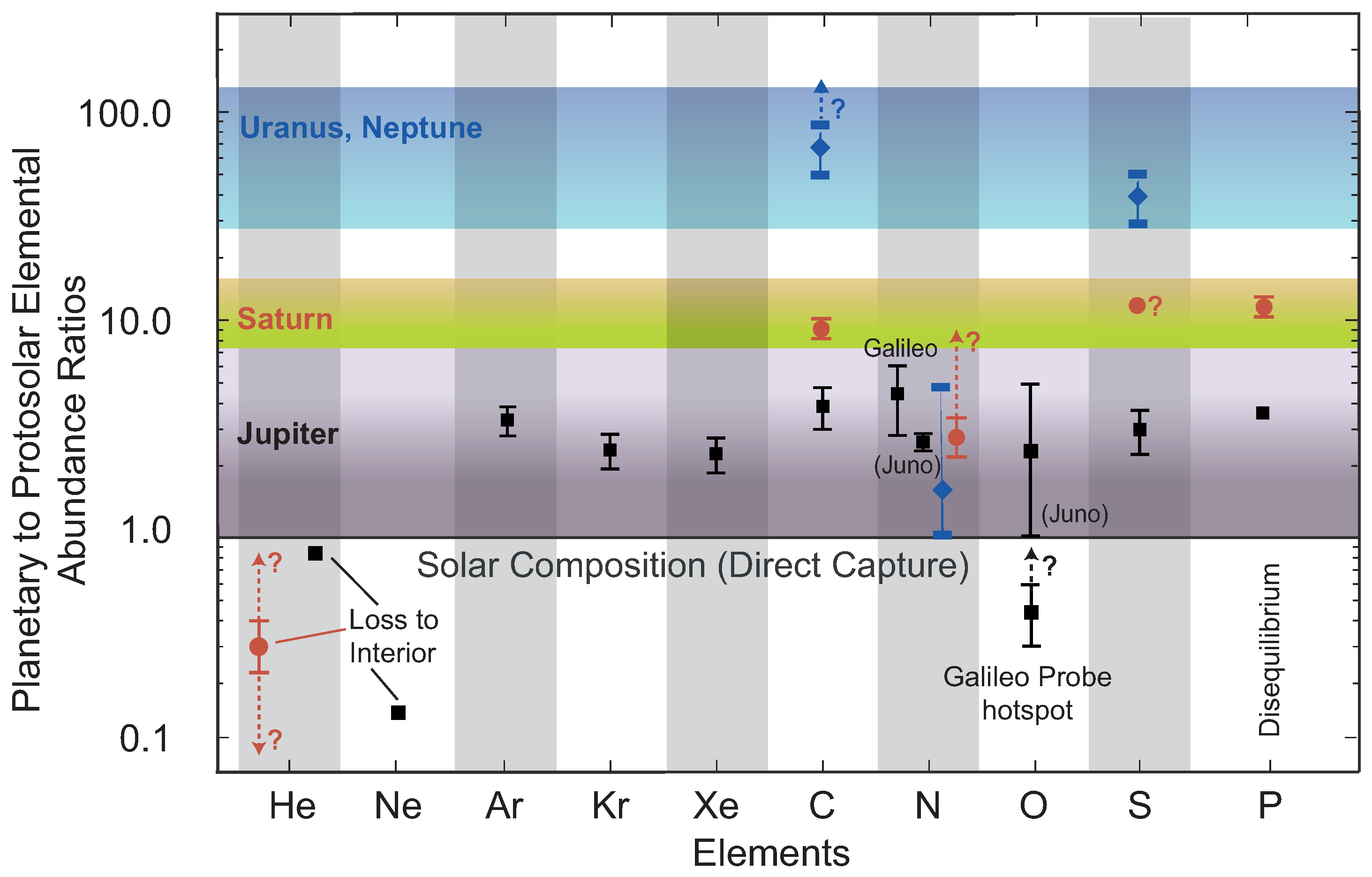
  • The approximately uniform enrichment of all elements heavier than hydrogen and helium (the astronomical “metals“) by a factor of ∼2–5 in Jupiter compared with the Sun;
  • The increasing level of enrichment of volatile elements over the proto-solar value with increasing heliocentric distance from Jupiter to Neptune (although only the carbon and sulfur enrichments have been measured accurately in the ice giants);
  • The increasing sulfur-to-nitrogen ratio with increasing heliocentric distance from Jupiter to Neptune.
These observations favor the core-accretion model of planet formation, and conditions in the outer disk that allow volatiles in planetesimals to be trapped as clathrate hydrates (Section 7.2). However, a key parameter that is needed to verify the amorphous vs. clathrated/crystalline ice scenarios as a way to differentiate planet formation models is the abundance of water; clathrate hydrate models require a three to four times larger enrichment in water over solar O than carbon (CH 4 ). Although water has been measured at Jupiter’s equator with Juno/MWR at an abundance between 1 and 5 × solar O, there are no data for the other three giant planets. Such detections remain challenging due, in part, to the high pressures at which water clouds form, which rule out potential in situ probe measurements. In addition, even if sub-water-cloud levels can be probed remotely, it remains a challenge to disentangle the effects by NH 3 , H 2 O, and potential other absorbers (e.g., alkalis). Although observations of CO in the planets’ stratospheres/upper tropospheres provide a promising technique, so far there is no hard evidence that O might be enhanced several times more than C in any of the planets (Section 7.3).
While the trapping of volatiles in clathrate hydrates is our favored outer-disk ice chemistry because it explains selective enhancements in volatiles and noble gases, it is worth considering whether the amorphous ice theory is also a possibility. One driver of the clathrate hydrate models is the measured N/S ratio on the planets. However, is the bulk abundance of nitrogen really depleted compared to other elements? Juno/VLA data show that dynamics deplete NH 3 in Jupiter’s upper atmosphere down to the 20–30 bar level. This might be the case on Saturn, too. In the ice giants, NH 3 could be locked up in a high-pressure super-ionic water ocean [212]. So the observed selective enhancements in the giant planets may simply be caused by our inability to probe deep enough into the planets’ atmospheres. Measurements of the noble gases may yield the final clues to settle the debate over crystalline vs. amorphous ice accretion. However, these can only be measured using probes.

Future Prospects

Although the continued technological progress in radio astronomy has been responsible for dramatic advances in our understanding of the giant planets, we still do not know the composition nor vertical structure of their deep atmospheres, which are key parameters to investigate heat transport and planet formation processes. With the planned upgrades to radio telescopes (discussed below) and future space missions, there is an excellent chance to learn more about the detailed thermal structure, global circulation, and vertical energy transport; the latter in particular in the ice giants through detailed characterization of methane condensation, since this gas is abundant enough to change the adiabatic profiles (dry ⟶ wet) and potentially inhibit convection.
Planned upgrades to radio telescopes and instrumentation in the next few decades promise to resolve, or at least further constrain, these questions. The ALMA development program’s Roadmap to 2030 [229] states the observatory’s intention to double their receiver bandwidth from 8 GHz to 16 GHz per polarization, making the wideband observations of planets twice as sensitive and permitting better characterization of the highly pressure-broadened spectral lines observed in planetary tropospheres. The Astronomy and Astrophysics Decadal Survey Astro2020 [230] endorsed the next-generation Very Large Array (ngVLA) project, a system of 263 antennas concentrated in the U.S. Southwest that promises high-fidelity imaging at ∼10 mas resolution over a spectral range from 1.2 to 116 GHz [231]. The order-of-magnitude higher sensitivity of this observatory will produce detailed maps of planetary atmospheres with ∼1-min integration times, eliminating the need for de-rotation algorithms and enabling feature tracking at radio wavelengths; see Refs. [12,232] for capabilities of and then destroyed higher upthe ngVLA for solar system science.
At lower frequencies (down to ∼50 MHz) the Square Kilometer Array (SKA), being built in Australia and South Africa, will be an excellent asset to probe the deep atmospheres of the giant planets at high spatial resolution and sensitivity [10,233]. Although probing Jupiter’s deep atmosphere required a spacecraft (Juno) to orbit inside the radiation belts, the deep atmospheres of the other three giant planets can be probed with the ngVLA and SKA. At a frequency of 1.5 GHz, the spatial resolution with the ngVLA on Uranus/Neptune is ∼2400/3600 km, close to Juno/MWR’s resolution on Jupiter [232]. With the SKA at 75 MHz, where we might probe below the solution cloud [232], the spatial resolution on Uranus/Neptune is ∼1100/1900 km [10], i.e., spatial resolutions that would be hard to beat even with an orbiter equipped with a radiometer such as Juno/MWR.
Although the new generation of radio telescopes will provide much-needed information on the giant planets’ deep atmosphere and perhaps the water abundance, and the James Webb Space Telescope will provide unique data at near- and mid-infrared wavelengths, other outstanding questions, such as the noble gas content and explorations of their magnetospheres, rings, and moons, do require orbiters and probes. We hence look forward to the JUpiter ICy moons Explorer (JUICE) [234] and Uranus Orbiter Probe (UOP) [223] missions to further our knowledge on atmospheric dynamics and formation theories.

Author Contributions

Conceptualization and formulation, I.d.P., C.M.M. and E.M.M.; methodology, I.d.P., E.M.M. and C.M.M.; software, I.d.P., C.M.M. and E.M.M.; investigation, I.d.P., C.M.M. and E.M.M.; writing—original draft preparation, I.d.P.; writing—review and editing, I.d.P., E.M.M. and C.M.M.; visualization, I.d.P., C.M.M. and E.M.M.; supervision, I.d.P.; project administration, I.d.P.; funding acquisition, I.d.P. All authors have read and agreed to the published version of the manuscript.

Funding

This research was funded by NSF Grant AST-1615004, and NASA’s Solar System Observations (SSO) awards 80NSSC18K1001 and NNX16AK14G to the University of California.

Data Availability Statement

This is a review paper, and for the original data the reader is referred to the original papers referenced in this review.

Acknowledgments

Over the years we have collaborated closely with R. J. Sault, David DeBoer and Bryan Butler, who all helped creating the radio maps and radiative transfer analysis presented in this review.

Conflicts of Interest

The authors declare no conflict of interest.

References

  1. Simon, A.A.; Wong, M.H.; Sromovsky, L.A.; Fletcher, L.N.; Fry, P.M. Giant Planet Atmospheres: Dynamics and Variability from UV to Near-IR Hubble and Adaptive Optics Imaging. Remote Sens. 2022, 14, 1518. [Google Scholar] [CrossRef]
  2. Roman, M.T.; Fletcher, L.N.; Orton, G.S.; Greathouse, T.K.; Moses, J.I.; Rowe-Gurney, N.; Irwin, P.G.J.; Antunano, A.; Sinclair, J.; Kasaba, Y.; et al. Sub-Seasonal Variation in Neptune’s Mid-Infrared Emission. arXiv 2021, arXiv:2112.00033. [Google Scholar]
  3. Bjoraker, G.L.; Wong, M.H.; de Pater, I.; Ádámkovics, M. Jupiter’s Deep Cloud Structure Revealed Using Keck Observations of Spectrally Resolved Line Shapes. Astrophys. J. 2015, 810, 122. [Google Scholar] [CrossRef]
  4. Bjoraker, G.L.; Wong, M.H.; de Pater, I.; Hewagama, T.; Ádámkovics, M.; Orton, G.S. The Gas Composition and Deep Cloud Structure of Jupiter’s Great Red Spot. Astron. J. 2018, 156, 101. [Google Scholar] [CrossRef]
  5. Bjoraker, G.L.; Wong, M.H.; de Pater, I.; Hewagama, T.; Ádámkovics, M. The Spatial Variation of Water Clouds, NH3, and H2O on Jupiter Using Keck Data at 5 Microns. Remote Sens. 2022, 14, 4567. [Google Scholar] [CrossRef]
  6. Noll, K.S.; Larson, H.P. The spectrum of Saturn from 1990 to 2230 cm−1: Abundances of AsH3, CH 3D, CO, GeH4, NH3, and PH3. Icarus 1991, 89, 168–189. [Google Scholar] [CrossRef]
  7. Fletcher, L.N.; Baines, K.H.; Momary, T.W.; Showman, A.P.; Irwin, P.G.J.; Orton, G.S.; Roos-Serote, M.; Merlet, C. Saturn’s tropospheric composition and clouds from Cassini/VIMS 4.6–5.1 μm nightside spectroscopy. Icarus 2011, 214, 510–533. [Google Scholar] [CrossRef]
  8. de Pater, I. The significance of microwave observations for the planets. Phys. Rep. 1991, 200, 1–50. [Google Scholar] [CrossRef]
  9. de Pater, I.; Romani, P.N.; Atreya, S.K. Possible microwave absorption by H2S gas in Uranus’ and Neptune’s atmospheres. Icarus 1991, 91, 220–233. [Google Scholar] [CrossRef]
  10. Butler, B.J.; Campbell, D.B.; de Pater, I.; Gary, D.E. Solar system science with SKA. New Astron. Rev. 2004, 48, 1511–1535. [Google Scholar] [CrossRef]
  11. de Pater, I.; Kurth, W.S. The Solar System at Radio Wavelengths. In Encyclopedia of the Solar System; Spohn, T., Breuer, D., Johnson, T.V., Eds.; Elsevier: Amsterdam, The Netherlands, 2014; pp. 1107–1132. [Google Scholar]
  12. de Pater, I.; Butler, B.; Sault, R.J.; Moullet, A.; Moeckel, C.; Tollefson, J.; de Kleer, K.; Gurwell, M.; Milam, S. Potential for Solar System Science with the ngVLA. In Science with a Next Generation Very Large Array; Murphy, E., Ed.; Astronomical Society of the Pacific Conference Series: San Francisco, CA, USA, 2018; Volume 517, p. 49. [Google Scholar]
  13. de Pater, I.; Sault, R.J.; Wong, M.H.; Fletcher, L.N.; DeBoer, D.; Butler, B. Jupiter’s ammonia distribution derived from VLA maps at 3–37 GHz. Icarus 2019, 322, 168–191. [Google Scholar] [CrossRef]
  14. Akins, A.; Hofstadter, M.; Butler, B.; Molter, E.; de Pater, I. Seasonal Change in the Deep Atmosphere of Uranus, 1981 to 2021. In Proceedings of the EGU General Assembly Conference Abstracts, Vienna, Austria, 23–27 May 2022; p. EGU22-6614. [Google Scholar] [CrossRef]
  15. Akins, A.; Hofstadter, M.; Butler, B.; Friedson, A.J.; Molter, E.; Parisi, M.; de Pater, I. Evidence of a polar cyclone on Uranus from VLA observations. GRL, 2023; submitted. [Google Scholar]
  16. Tollefson, J.; de Pater, I.; Molter, E.M.; Sault, R.J.; Butler, B.J.; Luszcz-Cook, S.; DeBoer, D. Neptune’s Spatial Brightness Temperature Variations from the VLA and ALMA. Planet. Sci. J. 2021, 2, 105. [Google Scholar] [CrossRef]
  17. Lewis, J.S. The clouds of Jupiter and the NH3H2O and NH3H2S systems. Icarus 1969, 10, 365–378. [Google Scholar] [CrossRef]
  18. Weidenschilling, S.J.; Lewis, J.S. Atmospheric and cloud structures of the Jovian planets. Icarus 1973, 20, 465–476. [Google Scholar] [CrossRef]
  19. Cornwell, T.J.; Perley, R.A. IAC Volume 131: Radio Interferometry: Theory, Techniques, and Applications. Int. Astron. Union Colloq. 1991, 131, f1–f11. [Google Scholar] [CrossRef]
  20. Synthesis Imaging in Radio Astronomy: A Collection of Lectures from the third NRAO Synthesis Imaging Summer School; Astronomical Society of the Pacific Conference Series: San Francisco, CA, USA, 1989; Volume 6.
  21. Synthesis Imaging in Radio Astronomy II; Astronomical Society of the Pacific Conference Series: San Francisco, CA, USA, 1999; Volume 180.
  22. Thompson, A.R.; Moran, J.M.; Swenson, G.W. Interferometry and Synthesis in Radio Astronomy; Springer Nature: Berlin/Heidelberg, Germany, 2017. [Google Scholar]
  23. Gibson, J.; Welch, W.J.; de Pater, I. Accurate jovian radio flux density measurements show ammonia to be subsaturated in the upper troposphere. Icarus 2005, 173, 439–446. [Google Scholar] [CrossRef]
  24. Sault, R.J.; Engel, C.; de Pater, I. Longitude-resolved imaging of Jupiter at λ = 2 cm. Icarus 2004, 168, 336–343. [Google Scholar] [CrossRef]
  25. de Pater, I.; Massie, S.T. Models of the millimeter-centimeter spectra of the giant planets. Icarus 1985, 62, 143–171. [Google Scholar] [CrossRef]
  26. DeBoer, D.R.; Steffes, P.G. Estimates of the Tropospheric Vertical Structure of Neptune Based on Microwave Radiative Transfer Studies. Icarus 1996, 123, 324–335. [Google Scholar] [CrossRef]
  27. de Pater, I.; Fletcher, L.N.; Luszcz-Cook, S.; DeBoer, D.; Butler, B.; Hammel, H.B.; Sitko, M.L.; Orton, G.; Marcus, P.S. Neptune’s global circulation deduced from multi-wavelength observations. Icarus 2014, 237, 211–238. [Google Scholar] [CrossRef]
  28. Janssen, M.A.; Oswald, J.E.; Brown, S.T.; Gulkis, S.; Levin, S.M.; Bolton, S.J.; Allison, M.D.; Atreya, S.K.; Gautier, D.; Ingersoll, A.P.; et al. MWR: Microwave Radiometer for the Juno Mission to Jupiter. Space Sci. Rev. 2017, 213, 139–185. [Google Scholar] [CrossRef]
  29. Hofstadter, M.D. Microwave Observations of Uranus. Ph.D. Thesis, California Institute of Technology, Pasadena, CA, USA, 1992. [Google Scholar]
  30. Atreya, S.K.; Romani, P.N. Photochemistry and clouds of Jupiter, Saturn and Uranus. In Recent Advances in Planetary Meteorology; Hunt, G.E., Ed.; Cambridge University Press: Cambridge, MA, USA, 1985; pp. 17–68. [Google Scholar]
  31. Atreya, S.K. Atmospheres and Ionospheres of the Outer Planets and their Satellites; Springer: Berlin/Heidelberg, Germany, 1986. [Google Scholar]
  32. de Pater, I.; DeBoer, D.; Marley, M.; Freedman, R.; Young, R. Retrieval of water in Jupiter’s deep atmosphere using microwave spectra of its brightness temperature. Icarus 2005, 173, 425–438. [Google Scholar] [CrossRef]
  33. Moeckel, C.; de Pater, I.; DeBoer, D. Ammonia Abundance Derived from Juno MWR and VLA Observations of Jupiter. Planet. Sci. J. 2023, 4, 25. [Google Scholar] [CrossRef]
  34. Lindal, G.F.; Wood, G.E.; Levy, G.S.; Anderson, J.D.; Sweetnam, D.N.; Hotz, H.B.; Buckles, B.J.; Holmes, D.P.; Doms, P.E.; Eshleman, V.R.; et al. The atmosphere of Jupiter: An analysis of the Voyager radio occulation measurements. J. Geophys. Res. 1981, 86, 8721–8727. [Google Scholar] [CrossRef]
  35. Lindal, G.F.; Sweetnam, D.N.; Eshleman, V.R. The atmosphere of Saturn - an analysis of the Voyager radio occultation measurements. Astron. J. 1985, 90, 1136–1146. [Google Scholar] [CrossRef]
  36. Lindal, G.F.; Lyons, J.R.; Sweetnam, D.N.; Eshleman, V.R.; Hinson, D.P.; Tyler, G.L. The atmosphere of Uranus: Results of radio occultation measurements with Voyager 2. J. Geophys. Res. 1987, 92, 14987–15001. [Google Scholar] [CrossRef]
  37. Lindal, G.F. The Atmosphere of Neptune: An Analysis of Radio Occultation Data Acquired with Voyager 2. Astron. J. 1992, 103, 967. [Google Scholar] [CrossRef]
  38. Seiff, A.; Kirk, D.B.; Knight, T.C.D.; Young, R.E.; Mihalov, J.D.; Young, L.A.; Milos, F.S.; Schubert, G.; Blanchard, R.C.; Atkinson, D. Thermal structure of Jupiter’s atmosphere near the edge of a 5-μm hot spot in the north equatorial belt. J. Geophys. Res. 1998, 103, 22857–22890. [Google Scholar] [CrossRef]
  39. Fletcher, L.N.; Orton, G.S.; Yanamandra-Fisher, P.; Fisher, B.M.; Parrish, P.D.; Irwin, P.G.J. Retrievals of atmospheric variables on the gas giants from ground-based mid-infrared imaging. Icarus 2009, 200, 154–175. [Google Scholar] [CrossRef]
  40. Fletcher, L.N.; de Pater, I.; Orton, G.S.; Hammel, H.B.; Sitko, M.L.; Irwin, P.G.J. Neptune at summer solstice: Zonal mean temperatures from ground-based observations, 2003–2007. Icarus 2014, 231, 146–167. [Google Scholar] [CrossRef]
  41. Orton, G.S.; Fletcher, L.N.; Encrenaz, T.; Leyrat, C.; Roe, H.G.; Fujiyoshi, T.; Pantin, E. Thermal imaging of Uranus: Upper-tropospheric temperatures one season after Voyager. Icarus 2015, 260, 94–102. [Google Scholar] [CrossRef]
  42. Fletcher, L.N.; Greathouse, T.K.; Orton, G.S.; Sinclair, J.A.; Giles, R.S.; Irwin, P.G.J.; Encrenaz, T. Mid-infrared mapping of Jupiter’s temperatures, aerosol opacity and chemical distributions with IRTF/TEXES. Icarus 2016, 278, 128–161. [Google Scholar] [CrossRef]
  43. Orton, G.S.; Gustafsson, M.; Burgdorf, M.; Meadows, V. Revised ab initio models for H 2-H 2 collision-induced absorption at low temperatures. Icarus 2007, 189, 544–549. [Google Scholar] [CrossRef]
  44. Devaraj, K.; Steffes, P.G.; Duong, D. The centimeter-wavelength opacity of ammonia under deep jovian conditions. Icarus 2014, 241, 165–179. [Google Scholar] [CrossRef]
  45. Deboer, D.R.; Steffes, P.G. Laboratory Measurements of the Microwave Properties of H 2S under Simulated Jovian Conditions with an Application to Neptune. Icarus 1994, 109, 352–366. [Google Scholar] [CrossRef]
  46. Hanley, T.R.; Steffes, P.G.; Karpowicz, B.M. A new model of the hydrogen and helium-broadened microwave opacity of ammonia based on extensive laboratory measurements. Icarus 2009, 202, 316–335. [Google Scholar] [CrossRef]
  47. Karpowicz, B.M.; Steffes, P.G. In search of water vapor on Jupiter: Laboratory measurements of the microwave properties of water vapor under simulated jovian conditions. Icarus 2011, 212, 210–223. [Google Scholar] [CrossRef]
  48. Bellotti, A.; Steffes, P.G.; Chinsomboom, G. Laboratory measurements of the 5–20 cm wavelength opacity of ammonia, water vapor, and methane under simulated conditions for the deep jovian atmosphere. Icarus 2016, 280, 255–267. [Google Scholar] [CrossRef]
  49. Bellotti, A.; Steffes, P.G.; Chinsomboon, G. Corrigendum to “Laboratory measurements of the 5–20 cm wavelength opacity of ammonia, water vapor, and methane under simulated conditions for the deep jovian atmosphere” [Icarus 280 (2016) 255-267]. Icarus 2017, 284, 491–492. [Google Scholar] [CrossRef]
  50. Briggs, F.H.; Sackett, P.D. Radio observations of Saturn as a probe of its atmosphere and cloud structure. Icarus 1989, 80, 77–103. [Google Scholar] [CrossRef]
  51. de Pater, I.; Mitchell, D.L. Radio Observations of the planets: The importance of laboratory measurements. J. Geophys. Res. 1993, 98, 5471–5490. [Google Scholar] [CrossRef]
  52. de Pater, I.; Dunn, D.; Romani, P.; Zahnle, K. Reconciling Galileo Probe Data and Ground-Based Radio Observations of Ammonia on Jupiter. Icarus 2001, 149, 66–78. [Google Scholar] [CrossRef]
  53. Ackerman, A.S.; Marley, M.S. Precipitating Condensation Clouds in Substellar Atmospheres. Astrophys. J. 2001, 556, 872–884. [Google Scholar] [CrossRef]
  54. Wong, M.H.; Atreya, S.K.; Kuhn, W.R.; Romani, P.N.; Mihalka, K.M. Fresh clouds: A parameterized updraft method for calculating cloud densities in one-dimensional models. Icarus 2015, 245, 273–281. [Google Scholar] [CrossRef]
  55. Irwin, P.G.J.; Teanby, N.A.; de Kok, R.; Fletcher, L.N.; Howett, C.J.A.; Tsang, C.C.C.; Wilson, C.F.; Calcutt, S.B.; Nixon, C.A.; Parrish, P.D. The NEMESIS planetary atmosphere radiative transfer and retrieval tool. J. Quant. Spectrosc. Radiat. Transf. 2008, 109, 1136–1150. [Google Scholar] [CrossRef]
  56. Foreman-Mackey, D.; Hogg, D.W.; Lang, D.; Goodman, J. emcee: The MCMC Hammer. Publ. Astron. Soc. Pac. 2013, 125, 306. [Google Scholar] [CrossRef]
  57. Molter, E.M.; de Pater, I.; Luszcz-Cook, S.; Tollefson, J.; Sault, R.J.; Butler, B.; de Boer, D. Tropospheric Composition and Circulation of Uranus with ALMA and the VLA. Planet. Sci. J. 2021, 2, 3. [Google Scholar] [CrossRef]
  58. Li, C.; de Pater, I.; Moeckel, C.; Sault, R.; Butler, B.; deBoer, D.; Zhang, Z. Long-lasting, deep effect of Saturn’s Giant Storms. Sci. Adv. 2023. [Google Scholar]
  59. Burke, B.F.; Franklin, K.L. Observations of a Variable Radio Source Associated with the Planet Jupiter. J. Geophys. Res. 1955, 60, 213–217. [Google Scholar] [CrossRef]
  60. Carr, T.D.; Desch, M.D. Recent decametric and hectometric observations of Jupiter. In Jupiter; University of Arizona Press: Tucson, AZ, USA, 1976; pp. 693–737. [Google Scholar]
  61. Carr, T.D.; Desch, M.D.; Alexander, J.K. Physics of the Jovian magnetosphere. 7. Phenomenology of magnetospheric radio emissions. In Physics of the Jovian Magnetosphere; Cambridge University Press: Cambridge, MA, USA, 1983; pp. 226–284. [Google Scholar]
  62. Mayer, C.H.; McCullough, T.P.; Sloanaker, R.M. Observation of Mar and Jupiter at a Wave Legth of 3.15 cm. Astrophys. J. 1958, 127, 11. [Google Scholar] [CrossRef]
  63. Radhakrishnan, V.; Roberts, J.A. Polarization and Angular Extent of the 960-Megacycle Radiation from Jupiter. Astron. J. 1960, 65, 498. [Google Scholar] [CrossRef]
  64. Morris, D.; Berge, G.L. Measurements of the polarization and angular extent of the decimetric radiation of Jupiter. Astrophys. J. 1962, 136, 276–282. [Google Scholar] [CrossRef]
  65. Berge, G.L.; Gulkis, S. Earth-based radio observations of Jupiter: Millimeter to meter wavelengths. In Jupiter; University of Arizona Press: Tucson, AZ, USA, 1976; pp. 621–692. [Google Scholar]
  66. de Pater, I. A comparison of the radio data and model calculations of Jupiter’s synchrotron radiation 1. The high energy electron distribution in Jupiter’s inner magnetosphere. J. Geophys. Res. 1981, 86, 3397–3422. [Google Scholar] [CrossRef]
  67. de Pater, I.; Schulz, M.; Brecht, S.H. Synchrotron evidence for Amalthea’s influence on Jupiter’s electron radiation belt. J. Geophys. Res. 1997, 102, 22043–22064. [Google Scholar] [CrossRef]
  68. Santos-Costa, D.; Bolton, S.J. Discussing the processes constraining the Jovian synchrotron radio emission’s features. Planet. Space Sci. 2008, 56, 326–345. [Google Scholar] [CrossRef]
  69. Roberts, J.A. The pitch angles of electrons in Jupiter’s radiation belt. PASA 1976, 3, 53–55. [Google Scholar] [CrossRef]
  70. Fillius, W.; McIlwain, C.; Mogro-Campero, A.; Steinberg, G. Evidence that pitch angle scattering is an important loss mechanism for energetic electrons in the inner radiation belt of Jupiter. Geophys. Res. Lett. 1976, 3, 33–36. [Google Scholar] [CrossRef]
  71. Santos-Costa, D.; Bourdarie, S.A. Modeling the inner Jovian electron radiation belt including non-equatorial particles. Planet. Space Sci. 2001, 49, 303–312. [Google Scholar] [CrossRef]
  72. de Pater, I.; Showalter, M.R.; Macintosh, B. Keck observations of the 2002 2003 jovian ring plane crossing. Icarus 2008, 195, 348–360. [Google Scholar] [CrossRef]
  73. de Pater, I. 21 CM maps of Jupiter’s radiation belts from all rotational aspects. Astron. Astrophys. 1980, 88, 175–183. [Google Scholar]
  74. Sault, R.J.; Oosterloo, T.; Dulk, G.A.; Leblanc, Y. The first three-dimensional reconstruction of a celestial object at radio wavelengths: Jupiter’s radiation belts. Astron. Astrophys. 1997, 324, 1190–1196. [Google Scholar]
  75. de Pater, I.; Sault, R.J. An intercomparison of three-dimensional reconstruction techniques using data and models of Jupiter’s synchrotron radiation. J. Geophys. Res. 1998, 103, 19973–19984. [Google Scholar] [CrossRef]
  76. Kloosterman, J.L.; Dunn, D.E.; de Pater, I. Jupiter’s Synchrotron Radiation Mapped with the Very Large Array from 1981 to 1998. Astrophys. J. Suppl. Ser. 2005, 161, 520–550. [Google Scholar] [CrossRef]
  77. Dunn, D.E.; de Pater, I.; Sault, R.J. Search for secular changes in the 3D profile of the synchrotron radiation around Jupiter. Icarus 2003, 165, 121–136. [Google Scholar] [CrossRef]
  78. Moore, K.M.; Yadav, R.K.; Kulowski, L.; Cao, H.; Bloxham, J.; Connerney, J.E.P.; Kotsiaros, S.; Jørgensen, J.L.; Merayo, J.M.G.; Stevenson, D.J.; et al. A complex dynamo inferred from the hemispheric dichotomy of Jupiter’s magnetic field. Nature 2018, 561, 76–78. [Google Scholar] [CrossRef]
  79. Klein, M.J.; Janssen, M.A.; Gulkis, S.; Olsen, E.T. Saturn’s microwave spectrum: Implications for the atmosphere and the rings. In NASA Conference Publication; National Aeronautics and Space Administration, Scientific and Technical Information Office: Washington, DC, USA, 1978; Volume 2068, pp. 195–216. [Google Scholar]
  80. Harrington, J.; de Pater, I.; Brecht, S.H.; Deming, D.; Meadows, V.; Zahnle, K.; Nicholson, P.D. Lessons from Shoemaker-Levy 9 about Jupiter and planetary impacts. In Jupiter. The Planet, Satellites and Magnetosphere; Bagenal, F., Dowling, T.E., McKinnon, W.B., Eds.; Cambridge University Press: Cambridge, MA, USA, 2004; Volume 1, pp. 159–184. [Google Scholar]
  81. Perley, R.A.; Chandler, C.J.; Butler, B.J.; Wrobel, J.M. The Expanded Very Large Array: A New Telescope for New Science. Astrophys. J. Lett. 2011, 739, L1. [Google Scholar] [CrossRef]
  82. Wrixon, G.T.; Welch, W.J.; Thornton, D.D. The Spectrum of Jupiter at Millimeter Wavelengths. Astrophys. J. 1971, 169, 171. [Google Scholar] [CrossRef]
  83. Asplund, M.; Grevesse, N.; Sauval, A.J.; Scott, P. The Chemical Composition of the Sun. Annu. Rev. Astron. Astrophys. 2009, 47, 481–522. [Google Scholar] [CrossRef]
  84. Weiland, J.L.; Odegard, N.; Hill, R.S.; Wollack, E.; Hinshaw, G.; Greason, M.R.; Jarosik, N.; Page, L.; Bennett, C.L.; Dunkley, J.; et al. Seven-year Wilkinson Microwave Anisotropy Probe (WMAP) Observations: Planets and Celestial Calibration Sources. Astrophys. J. Suppl. Ser. 2011, 192, 19. [Google Scholar] [CrossRef]
  85. Karim, R.L.; DeBoer, D.; de Pater, I.; Keating, G.K. A Wideband Self-consistent Disk-averaged Spectrum of Jupiter Near 30 GHz and Its Implications for NH3 Saturation in the Upper Troposphere. Astron. J. 2018, 155, 129. [Google Scholar] [CrossRef]
  86. Moeckel, C.; Janssen, M.; de Pater, I. A re-analysis of the Jovian radio emission as seen by Cassini-RADAR and evidence for time variability. Icarus 2019, 321, 994–1012. [Google Scholar] [CrossRef]
  87. Planck Collaboration; Akrami, Y.; Ashdown, M.; Aumont, J.; Baccigalupi, C.; Ballardini, M.; Banday, A.J.; Barreiro, R.B.; Bartolo, N.; Basak, S.; et al. Planck intermediate results. LII. Planet flux densities. Astron. Astrophys. 2017, 607, A122. [Google Scholar] [CrossRef]
  88. Maris, M.; Romelli, E.; Tomasi, M.; Gregorio, A.; Sandri, M.; Galeotta, S.; Tavagnacco, D.; Frailis, M.; Maggio, G.; Zacchei, A. Revised planet brightness temperatures using the Planck/LFI 2018 data release. Astron. Astrophys. 2021, 647, A104. [Google Scholar] [CrossRef]
  89. Li, C.; Ingersoll, A.; Janssen, M.; Levin, S.; Bolton, S.; Adumitroaie, V.; Allison, M.; Arballo, J.; Bellotti, A.; Brown, S.; et al. The distribution of ammonia on Jupiter from a preliminary inversion of Juno microwave radiometer data. Geophys. Res. Lett. 2017, 44, 5317–5325. [Google Scholar] [CrossRef]
  90. Folkner, W.M.; Woo, R.; Nandi, S. Ammonia abundance in Jupiter’s atmosphere derived from the attenuation of the Galileo probe’s radio signal. J. Geophys. Res. 1998, 103, 22847–22856. [Google Scholar] [CrossRef]
  91. Niemann, H.B.; Atreya, S.K.; Carignan, G.R.; Donahue, T.M.; Haberman, J.A.; Harpold, D.N.; Hartle, R.E.; Hunten, D.M.; Kasprzak, W.T.; Mahaffy, P.R.; et al. The composition of the Jovian atmosphere as determined by the Galileo probe mass spectrometer. J. Geophys. Res. 1998, 103, 22831–22846. [Google Scholar] [CrossRef]
  92. Wong, M.H.; Mahaffy, P.R.; Atreya, S.K.; Niemann, H.B.; Owen, T.C. Updated Galileo probe mass spectrometer measurements of carbon, oxygen, nitrogen, and sulfur on Jupiter. Icarus 2004, 171, 153–170. [Google Scholar] [CrossRef]
  93. Showman, A.P.; de Pater, I. Dynamical implications of Jupiter’s tropospheric ammonia abundance. Icarus 2005, 174, 192–204. [Google Scholar] [CrossRef]
  94. de Pater, I.; Jaffe, W.J. Very large array observations of Jupiter’s nonthermal radiation. Astrophys. J. Suppl. Ser. 1984, 54, 405–419. [Google Scholar] [CrossRef]
  95. de Pater, I.; Dickel, J.R. Jupiter’s Zone-Belt Structure of Radio Wavelengths. I. Observations. Astrophys. J. 1986, 308, 459. [Google Scholar] [CrossRef]
  96. de Pater, I. Jupiter’s zone-belt structure at radio wavelengths. II. Comparison of observations with model atmosphere calculations. Icarus 1986, 68, 344–365. [Google Scholar] [CrossRef]
  97. de Pater, I.; Sault, R.J.; Butler, B.; DeBoer, D.; Wong, M.H. Peering through Jupiter’s clouds with radio spectral imaging. Science 2016, 352, 1198–1201. [Google Scholar] [CrossRef] [PubMed]
  98. de Pater, I.; Sault, R.J.; Moeckel, C.; Moullet, A.; Wong, M.H.; Goullaud, C.; DeBoer, D.; Butler, B.J.; Bjoraker, G.; Ádámkovics, M.; et al. First ALMA Millimeter-wavelength Maps of Jupiter, with a Multiwavelength Study of Convection. Astron. J. 2019, 158, 139. [Google Scholar] [CrossRef]
  99. Allison, M. Planetary waves in Jupiter’s equatorial atmosphere. Icarus 1990, 83, 282–307. [Google Scholar] [CrossRef]
  100. Ortiz, J.L.; Orton, G.S.; Friedson, A.J.; Stewart, S.T.; Fisher, B.M.; Spencer, J.R. Evolution and persistence of 5-μm hot spots at the Galileo probe entry latitude. J. Geophys. Res. 1998, 103, 23051–23069. [Google Scholar] [CrossRef]
  101. Showman, A.P.; Dowling, T.E. Nonlinear Simulations of Jupiter’s 5-Micron Hot Spots. Science 2000, 289, 1737–1740. [Google Scholar] [CrossRef]
  102. Friedson, A.J. Water, ammonia, and H 2S mixing ratios in Jupiter’s five-micron hot spots: A dynamical model. Icarus 2005, 177, 1–17. [Google Scholar] [CrossRef]
  103. Cook, J.J.; Cross, L.G.; Bair, M.E.; Arnold, C.B. Radio Detection of the Planet Saturn. Nature 1960, 188, 393–394. [Google Scholar] [CrossRef]
  104. Drake, F.D. Microwave Spectrum of Saturn. Nature 1962, 195, 893–894. [Google Scholar] [CrossRef]
  105. Wrixon, G.T.; Welch, W.J. The Millimeter Wave Spectrum of Saturn. Icarus 1970, 13, 163–172. [Google Scholar] [CrossRef]
  106. de Pater, I.; Dickel, J.R. Multifrequency radio observations of Saturn at ring inclination angles between 5 and 26 degrees. Icarus 1991, 94, 474–492. [Google Scholar] [CrossRef]
  107. van der Tak, F.; de Pater, I.; Silva, A.; Millan, R. Time Variability in the Radio Brightness Distribution of Saturn. Icarus 1999, 142, 125–147. [Google Scholar] [CrossRef]
  108. Dunn, D.E.; Molnar, L.A.; Fix, J.D. More Microwave Observations of Saturn: Modeling the Ring with a Monte Carlo Radiative Transfer Code. Icarus 2002, 160, 132–160. [Google Scholar] [CrossRef]
  109. Zhang, Z.; Hayes, A.G.; de Pater, I.; Dunn, D.E.; Janssen, M.A.; Nicholson, P.D.; Cuzzi, J.N.; Butler, B.J.; Sault, R.J.; Chatterjee, S. VLA multi-wavelength microwave observations of Saturn’s C and B rings. Icarus 2019, 317, 518–548. [Google Scholar] [CrossRef]
  110. Schloerb, F.P.; Muhleman, D.O.; Berge, G.L. Interferometric observations of Saturn and its rings at a wavelength of 3 3.71 cm. Icarus 1979, 39, 214–231. [Google Scholar] [CrossRef]
  111. de Pater, I.; Dickel, J.R. VLA observations of Saturn at 1.3, 2, and 6 cm. Icarus 1982, 50, 88–102. [Google Scholar] [CrossRef]
  112. Grossman, A.W.; Muhleman, D.O.; Berge, G.L. High-Resolution Microwave Images of Saturn. Science 1989, 245, 1211–1215. [Google Scholar] [CrossRef]
  113. Dunn, D.E.; de Pater, I.; Molnar, L.A. Examining the wake structure in Saturn’s rings from microwave observations over varying ring opening angles and wavelengths. Icarus 2007, 192, 56–76. [Google Scholar] [CrossRef]
  114. de Pater, I.; Dickel, J.R. New information on Saturn and its rings from multi-frequency VLA data. Adv. Space Res. 1983, 3, 39–41. [Google Scholar] [CrossRef]
  115. Janssen, M.A.; Ingersoll, A.P.; Allison, M.D.; Gulkis, S.; Laraia, A.L.; Baines, K.H.; Edgington, S.G.; Anderson, Y.Z.; Kelleher, K.; Oyafuso, F.A. Saturn’s thermal emission at 2.2-cm wavelength as imaged by the Cassini RADAR radiometer. Icarus 2013, 226, 522–535. [Google Scholar] [CrossRef]
  116. Sánchez-Lavega, A.; del Río-Gaztelurrutia, T.; Hueso, R.; Gómez-Forrellad, J.M.; Sanz-Requena, J.F.; Legarreta, J.; García-Melendo, E.; Colas, F.; Lecacheux, J.; Fletcher, L.N.; et al. Deep winds beneath Saturn’s upper clouds from a seasonal long-lived planetary-scale storm. Nature 2011, 475, 71–74. [Google Scholar] [CrossRef] [PubMed]
  117. Fletcher, L.N.; Hesman, B.E.; Irwin, P.G.J.; Baines, K.H.; Momary, T.W.; Sanchez-Lavega, A.; Flasar, F.M.; Read, P.L.; Orton, G.S.; Simon-Miller, A.; et al. Thermal Structure and Dynamics of Saturn’s Northern Springtime Disturbance. Science 2011, 332, 1413. [Google Scholar] [CrossRef] [PubMed]
  118. Laraia, A.L.; Ingersoll, A.P.; Janssen, M.A.; Gulkis, S.; Oyafuso, F.; Allison, M. Analysis of Saturn’s thermal emission at 2.2-cm wavelength: Spatial distribution of ammonia vapor. Icarus 2013, 226, 641–654. [Google Scholar] [CrossRef]
  119. Sanchez-Lavega, A.; Colas, F.; Lecacheux, J.; Laques, P.; Miyazaki, I.; Parker, D. The Great White Spot and disturbances in Saturn’s equatorial atmosphere during 1990. Nature 1991, 353, 397–401. [Google Scholar] [CrossRef]
  120. Beebe, R.F.; Barnet, C.; Sada, P.V.; Murrell, A.S. The onset and growth of the 1990 equatorial disturbance on Saturn. Icarus 1992, 95, 163–172. [Google Scholar] [CrossRef]
  121. Li, C.; Ingersoll, A.P. Moist convection in hydrogen atmospheres and the frequency of Saturn’s giant storms. Nat. Geosci. 2015, 8, 398–403. [Google Scholar] [CrossRef]
  122. Allison, M.; Godfrey, D.A.; Beebe, R.F. A Wave Dynamical Interpretation of Saturn’s Polar Hexagon. Science 1990, 247, 1061–1063. [Google Scholar] [CrossRef]
  123. Dunn, D.E.; Molnar, L.A.; Fix, J.D. VLA Observations of Saturn’s Rings at Saturnian Equinox. In Proceedings of the AAS/Division for Planetary Sciences Meeting Abstracts #28, Tucson, AZ, USA, 23–26 October 1996; Volume 28, p. 18.04. [Google Scholar]
  124. Julian, W.H.; Toomre, A. Non-Axisymmetric Responses of Differentially Rotating Disks of Stars. Astrophys. J. 1966, 146, 810. [Google Scholar] [CrossRef]
  125. Salo, H. Gravitational wakes in Saturn’s rings. Nature 1992, 359, 619–621. [Google Scholar] [CrossRef]
  126. Salo, H. Simulations of dense planetary rings. III. Self-gravitating identical particles. Icarus 1995, 117, 287–312. [Google Scholar] [CrossRef]
  127. Zhang, Z.; Hayes, A.G.; Janssen, M.A.; Nicholson, P.D.; Cuzzi, J.N.; de Pater, I.; Dunn, D.E. Exposure age of Saturn’s A and B rings, and the Cassini Division as suggested by their non-icy material content. Icarus 2017, 294, 14–42. [Google Scholar] [CrossRef]
  128. Zhang, Z.; Hayes, A.G.; Janssen, M.A.; Nicholson, P.D.; Cuzzi, J.N.; de Pater, I.; Dunn, D.E.; Estrada, P.R.; Hedman, M.M. Cassini microwave observations provide clues to the origin of Saturn’s C ring. Icarus 2017, 281, 297–321. [Google Scholar] [CrossRef]
  129. Kellermann, K.I. The thermal radio emission from Mercury, Venus, Mars, Saturn, and Uranus. Icarus 1966, 5, 478–490. [Google Scholar] [CrossRef]
  130. Gulkis, S.; Janssen, M.A.; Olsen, E.T. Evidence for the depletion of ammonia in the Uranus atmosphere. Icarus 1978, 34, 10–19. [Google Scholar] [CrossRef]
  131. Gulkis, S.; Olsen, E.T.; Klein, M.J.; Thompson, T.J. Uranus: Variability of the Microwave Spectrum. Science 1983, 221, 453–455. [Google Scholar] [CrossRef]
  132. Gulkis, S.; Depater, I. A review of the millimeter and centimeter observations of Uranus. In NASA Conference Publication; Bergstralh, J.T., Ed.; National Aeronautics and Space Administration, Scientific and Technical Information Office: Washington, DC, USA, 1984; Volume 2330, pp. 225–262. [Google Scholar]
  133. Jaffe, W.J.; Berge, G.L.; Owen, T.; Caldwell, J. Uranus: Microwave Images. Science 1984, 225, 619–621. [Google Scholar] [CrossRef]
  134. de Pater, I.; Gulkis, S. VLA observations of Uranus at 1.3-20 cm. Icarus 1988, 75, 306–323. [Google Scholar] [CrossRef]
  135. Klein, M.J.; Hofstadter, M.D. Long-term variations in the microwave brightness temperature of the Uranus atmosphere. Icarus 2006, 184, 170–180. [Google Scholar] [CrossRef]
  136. Lockwood, G.W. Final compilation of photometry of Uranus and Neptune, 1972-2016. Icarus 2019, 324, 77–85. [Google Scholar] [CrossRef]
  137. de Pater, I.; Romani, P.N.; Atreya, S.K. Uranus deep atmosphere revealed. Icarus 1989, 82, 288–313. [Google Scholar] [CrossRef]
  138. Irwin, P.G.J.; Toledo, D.; Garland, R.; Teanby, N.A.; Fletcher, L.N.; Orton, G.A.; Bézard, B. Detection of hydrogen sulfide above the clouds in Uranus’s atmosphere. Nat. Astron. 2018, 2, 420–427. [Google Scholar] [CrossRef]
  139. Hofstadter, M.D.; Butler, B.J. Seasonal change in the deep atmosphere of Uranus. Icarus 2003, 165, 168–180. [Google Scholar] [CrossRef]
  140. Hofstadter, M.D.; Berge, G.L.; Muhleman, D.O. Vertical motions in the Uranian atmosphere: An analysis of radio observations. Icarus 1990, 84, 261–267. [Google Scholar] [CrossRef]
  141. Molter, E.; de Pater, I.; Luszcz-Cook, S.; Hueso, R.; Tollefson, J.; Alvarez, C.; Sánchez-Lavega, A.; Wong, M.H.; Hsu, A.I.; Sromovsky, L.A.; et al. Analysis of Neptune’s 2017 bright equatorial storm. Icarus 2019, 321, 324–345. [Google Scholar] [CrossRef]
  142. Kellermann, K.I.; Pauliny-Toth, I.I.K. Observations of the Radio Emission of Uranus, Neptune, and Other Planets at 1.9 CM. Astrophys. J. 1966, 145, 954. [Google Scholar] [CrossRef]
  143. de Pater, I.; Richmond, M. Neptune’s microwave spectrum from 1 mm to 20 cm. Icarus 1989, 80, 1–13. [Google Scholar] [CrossRef]
  144. Hofstadter, M.D. Microwave Imaging of Neptune’s Troposphere. In Proceedings of the AAS/Division for Planetary Sciences Meeting Abstracts #25, Boulder, CO, USA, 18–22 October 1993; Volume 25, p. 18.05. [Google Scholar]
  145. Irwin, P.G.J.; Toledo, D.; Garland, R.; Teanby, N.A.; Fletcher, L.N.; Orton, G.S.; Bézard, B. Probable detection of hydrogen sulphide (H2S) in Neptune’s atmosphere. Icarus 2019, 321, 550–563. [Google Scholar] [CrossRef]
  146. Butler, B.J.; Hofstadter, M.; Gurwell, M.; Orton, G.; Norwood, J. The Deep Atmosphere of Neptune From EVLA Observations. In Proceedings of the AAS/Division for Planetary Sciences Meeting Abstracts #44, Reno, NV, USA, 14–19 October 2012; Volume 44, p. 504.06. [Google Scholar]
  147. Tollefson, J.; de Pater, I.; Luszcz-Cook, S.; DeBoer, D. Neptune’s Latitudinal Variations as Viewed with ALMA. Astron. J. 2019, 157, 251. [Google Scholar] [CrossRef]
  148. Genio, A.D.D.; Achterberg, R.K.; Baines, K.H.; Flasar, F.M.; Read, P.L.; Sánchez-Lavega, A.; Showman, A.P. Saturn atmospheric structure and dynamics. In Saturn from Cassini-Huygens; Springer: Berlin/Heidelberg, Germany, 2009; pp. 113–159. [Google Scholar]
  149. Sromovsky, L.A.; Karkoschka, E.; Fry, P.M.; Hammel, H.B.; de Pater, I.; Rages, K. Methane depletion in both polar regions of Uranus inferred from HST/STIS and Keck/NIRC2 observations. Icarus 2014, 238, 137–155. [Google Scholar] [CrossRef]
  150. Showman, A.P.; Ingersoll, A.P.; Achterberg, R.; Kaspi, Y. The global atmospheric circulation of Saturn. In Saturn in the 21st Century; Cambridge University Press: Cambridge, UK, 2018; Volume 20, p. 295. [Google Scholar]
  151. Fletcher, L.N.; de Pater, I.; Orton, G.S.; Hofstadter, M.D.; Irwin, P.G.J.; Roman, M.T.; Toledo, D. Ice Giant Circulation Patterns: Implications for Atmospheric Probes. Space Sci. Rev. 2020, 216, 21. [Google Scholar] [CrossRef] [PubMed]
  152. Fletcher, L.N.; Kaspi, Y.; Guillot, T.; Showman, A.P. How Well Do We Understand the Belt/Zone Circulation of Giant Planet Atmospheres? Space Sci. Rev. 2020, 216, 30. [Google Scholar] [CrossRef] [PubMed]
  153. Fletcher, L.N.; Oyafuso, F.A.; Allison, M.; Ingersoll, A.; Li, L.; Kaspi, Y.; Galanti, E.; Wong, M.H.; Orton, G.S.; Duer, K.; et al. Jupiter’s Temperate Belt/Zone Contrasts Revealed at Depth by Juno Microwave Observations. J. Geophys. Res. (Planets) 2021, 126, e06858. [Google Scholar] [CrossRef]
  154. Conrath, B.J.; Gierasch, P.J. Global variation of the para hydrogen fraction in Jupiter’s atmosphere and implications for dynamics on the outer planets. Icarus 1984, 57, 184–204. [Google Scholar] [CrossRef]
  155. Wang, D.; Lunine, J.I.; Mousis, O. Modeling the disequilibrium species for Jupiter and Saturn: Implications for Juno and Saturn entry probe. Icarus 2016, 276, 21–38. [Google Scholar] [CrossRef]
  156. Marcus, P.S.; Tollefson, J.; Wong, M.H.; Pater, I.d. An equatorial thermal wind equation: Applications to Jupiter. Icarus 2019, 324, 198–223. [Google Scholar] [CrossRef]
  157. Tollefson, J.; Pater, I.d.; Marcus, P.S.; Luszcz-Cook, S.; Sromovsky, L.A.; Fry, P.M.; Fletcher, L.N.; Wong, M.H. Vertical wind shear in Neptune’s upper atmosphere explained with a modified thermal wind equation. Icarus 2018, 311, 317–339. [Google Scholar] [CrossRef]
  158. Gierasch, P.J.; Conrath, B.J.; Magalhães, J.A. Zonal mean properties of Jupiter’s upper troposphere from voyager infrared observations. Icarus 1986, 67, 456–483. [Google Scholar] [CrossRef]
  159. West, R.A.; Friedson, A.J.; Appleby, J.F. Jovian large-scale stratospheric circulation. Icarus 1992, 100, 245–259. [Google Scholar] [CrossRef]
  160. Moreno, F.; Sedano, J. Radiative Balance and Dynamics in the Stratosphere of Jupiter: Results from a Latitude-Dependent Aerosol Heating Model. Icarus 1997, 130, 36–48. [Google Scholar] [CrossRef]
  161. Ingersoll, A.P.; Gierasch, P.J.; Banfield, D.; Vasavada, A.R.; Galileo Imaging Team. Moist convection as an energy source for the large-scale motions in Jupiter’s atmosphere. Nature 2000, 403, 630–632. [Google Scholar] [CrossRef] [PubMed]
  162. Pirraglia, J.A.; Conrath, B.J.; Allison, M.D.; Gierasch, P.J. Thermal structure and dynamics of Saturn and Jupiter. Nature 1981, 292, 677–679. [Google Scholar] [CrossRef]
  163. Conrath, B.J.; Flasar, F.M.; Pirraglia, J.A.; Gierasch, P.J.; Hunt, G.E. Thermal structure and dynamics of the Jovian atmosphere 2. visible cloud features. J. Geophys. Res. 1981, 86, 8769–8775. [Google Scholar] [CrossRef]
  164. Conrath, B.J.; Gierasch, P.J.; Ustinov, E.A. Thermal Structure and Para Hydrogen Fraction on the Outer Planets from Voyager IRIS Measurements. Icarus 1998, 135, 501–517. [Google Scholar] [CrossRef]
  165. Atkinson, D.H.; Pollack, J.B.; Seiff, A. The Galileo probe Doppler wind experiment: Measurement of the deep zonal winds on Jupiter. J. Geophys. Res. 1998, 103, 22911–22928. [Google Scholar] [CrossRef]
  166. Sánchez-Lavega, A.; Hueso, R.; Pérez-Hoyos, S. The three-dimensional structure of Saturn’s equatorial jet at cloud level. Icarus 2007, 187, 510–519. [Google Scholar] [CrossRef]
  167. Fletcher, L.N.; Orton, G.S.; Teanby, N.A.; Irwin, P.G.J. Phosphine on Jupiter and Saturn from Cassini/CIRS. Icarus 2009, 202, 543–564. [Google Scholar] [CrossRef]
  168. Conrath, B.J.; Gierasch, P.J.; Herter, T.; Wang, J. Temperature and para hydrogen gradients on Jupiter observed from the FORCAST camera on SOFIA. Icarus 2018, 315, 1–6. [Google Scholar] [CrossRef]
  169. Fletcher, L.N.; de Pater, I.; Reach, W.T.; Wong, M.; Orton, G.S.; Irwin, P.G.J.; Gehrz, R.D. Jupiter’s para-H2 distribution from SOFIA/FORCAST and Voyager/IRIS 17-37 μm spectroscopy. Icarus 2017, 286, 223–240. [Google Scholar] [CrossRef]
  170. de Pater, I.; Fletcher, L.N.; Reach, W.T.; Goullaud, C.; Orton, G.S.; Wong, M.H.; Gehrz, R.D. SOFIA Observations of Variability in Jupiter’s Para-H2 Distribution and Subsurface Emission Characteristics of the Galilean Satellites. Planet. Sci. J. 2021, 2, 226. [Google Scholar] [CrossRef]
  171. Massie, S.T.; Hunten, D.M. Conversion of para and ortho hydrogen in the Jovian planets. Icarus 1982, 49, 213–226. [Google Scholar] [CrossRef]
  172. Karkoschka, E.; Tomasko, M. Saturn’s vertical and latitudinal cloud structure 1991 2004 from HST imaging in 30 filters. Icarus 2005, 179, 195–221. [Google Scholar] [CrossRef]
  173. Giles, R.S.; Fletcher, L.N.; Irwin, P.G.J. Latitudinal variability in Jupiter’s tropospheric disequilibrium species: GeH4, AsH3 and PH3. Icarus 2017, 289, 254–269. [Google Scholar] [CrossRef]
  174. Duer, K.; Gavriel, N.; Galanti, E.; Kaspi, Y.; Fletcher, L.N.; Guillot, T.; Bolton, S.J.; Levin, S.M.; Atreya, S.K.; Grassi, D.; et al. Evidence for Multiple Ferrel-Like Cells on Jupiter. Geophys. Res. Lett. 2021, 48, e95651. [Google Scholar] [CrossRef]
  175. Borucki, W.J.; Williams, M.A. Lightning in the Jovian water cloud. J. Geophys. Res. 1986, 91, 9893–9903. [Google Scholar] [CrossRef]
  176. Little, B.; Anger, C.D.; Ingersoll, A.P.; Vasavada, A.R.; Senske, D.A.; Breneman, H.H.; Borucki, W.J.; Galileo SSI Team. Galileo Images of Lightning on Jupiter. Icarus 1999, 142, 306–323. [Google Scholar] [CrossRef]
  177. Dyudina, U.A.; Ingersoll, A.P.; Vasavada, A.R.; Ewald, S.P.; Galileo SSI Team. Monte Carlo Radiative Transfer Modeling of Lightning Observed in Galileo Images of Jupiter. Icarus 2002, 160, 336–349. [Google Scholar] [CrossRef]
  178. Porco, C.C.; West, R.A.; McEwen, A.; Del Genio, A.D.; Ingersoll, A.P.; Thomas, P.; Squyres, S.; Dones, L.; Murray, C.D.; Johnson, T.V.; et al. Cassini Imaging of Jupiter’s Atmosphere, Satellites, and Rings. Science 2003, 299, 1541–1547. [Google Scholar] [CrossRef]
  179. Brown, S.; Janssen, M.; Adumitroaie, V.; Atreya, S.; Bolton, S.; Gulkis, S.; Ingersoll, A.; Levin, S.; Li, C.; Li, L.; et al. Prevalent lightning sferics at 600 megahertz near Jupiter’s poles. Nature 2018, 558, 87–90. [Google Scholar] [CrossRef]
  180. Dyudina, U.A.; Ingersoll, A.P.; Ewald, S.P.; Porco, C.C.; Fischer, G.; Yair, Y. Saturn’s visible lightning, its radio emissions, and the structure of the 2009–2011 lightning storms. Icarus 2013, 226, 1020–1037. [Google Scholar] [CrossRef]
  181. Fletcher, L.N.; Orton, G.S.; Rogers, J.H.; Giles, R.S.; Payne, A.V.; Irwin, P.G.J.; Vedovato, M. Moist convection and the 2010–2011 revival of Jupiter’s South Equatorial Belt. Icarus 2017, 286, 94–117. [Google Scholar] [CrossRef]
  182. Guillot, T.; Stevenson, D.J.; Atreya, S.K.; Bolton, S.J.; Becker, H.N. Storms and the Depletion of Ammonia in Jupiter: I. Microphysics of “Mushballs”. J. Geophys. Res. (Planets) 2020, 125, e06403. [Google Scholar] [CrossRef]
  183. Guillot, T. Condensation of Methane, Ammonia, and Water and the Inhibition of Convection in Giant Planets. Science 1995, 269, 1697–1699. [Google Scholar] [CrossRef]
  184. Leconte, J.; Selsis, F.; Hersant, F.; Guillot, T. Condensation-inhibited convection in hydrogen-rich atmospheres. Stability against double-diffusive processes and thermal profiles for Jupiter, Saturn, Uranus, and Neptune. Astron. Astrophys. 2017, 598, A98. [Google Scholar] [CrossRef]
  185. Ge, H.; Li, C.; Zhang, X. Exploring the role of water in Jupiter’s weather layer: Implication to the evolution and interior of gas giants. In Proceedings of the AAS/Division for Planetary Sciences Meeting Abstracts, London, UK, 2–7 October 2022; Volume 54, p. 302.02. [Google Scholar]
  186. Fletcher, L.N. Cycles of activity in the Jovian atmosphere. Geophys. Res. Lett. 2017, 44, 4725–4729. [Google Scholar] [CrossRef]
  187. Conrath, B.J.; Flasar, F.M.; Gierasch, P.J. Thermal structure and dynamics of Neptune’s atmosphere from Voyager measurements. J. Geophys. Res. 1991, 96, 18931–18939. [Google Scholar] [CrossRef]
  188. Flasar, F.M.; Conrath, B.J.; Gierasch, P.J.; Pirraglia, J.A. Voyager infrared observations of Uranus’ atmosphere: Thermal structure and dynamics. J. Geophys. Res. 1987, 92, 15011–15018. [Google Scholar] [CrossRef]
  189. Sromovsky, L.A.; Fry, P.M.; Hammel, H.B.; de Pater, I.; Rages, K.A. Post-equinox dynamics and polar cloud structure on Uranus. Icarus 2012, 220, 694–712. [Google Scholar] [CrossRef]
  190. Luszcz-Cook, S.H.; de Pater, I.; Ádámkovics, M.; Hammel, H.B. Seeing double at Neptune’s south pole. Icarus 2010, 208, 938–944. [Google Scholar] [CrossRef]
  191. Mizuno, H. Formation of the Giant Planets. Prog. Theor. Phys. 1980, 64, 544–557. [Google Scholar] [CrossRef]
  192. Stevenson, D.J. Formation of the giant planets. Planet. Space Sci. 1982, 30, 755–764. [Google Scholar] [CrossRef]
  193. Pollack, J.B.; Hubickyj, O.; Bodenheimer, P.; Lissauer, J.J.; Podolak, M.; Greenzweig, Y. Formation of the Giant Planets by Concurrent Accretion of Solids and Gas. Icarus 1996, 124, 62–85. [Google Scholar] [CrossRef]
  194. de Pater, I.; Lissauer, J.J. Planetary Sciences; Cambridge University Press: Cambridge, MA, USA, 2015. [Google Scholar]
  195. Helled, R.; Stevenson, D.J.; Lunine, J.I.; Bolton, S.J.; Nettelmann, N.; Atreya, S.; Guillot, T.; Militzer, B.; Miguel, Y.; Hubbard, W.B. Revelations on Jupiter’s formation, evolution and interior: Challenges from Juno results. Icarus 2022, 378, 114937. [Google Scholar] [CrossRef]
  196. Wahl, S.M.; Hubbard, W.B.; Militzer, B.; Guillot, T.; Miguel, Y.; Movshovitz, N.; Kaspi, Y.; Helled, R.; Reese, D.; Galanti, E.; et al. Comparing Jupiter interior structure models to Juno gravity measurements and the role of a dilute core. Geophys. Res. Lett. 2017, 44, 4649–4659. [Google Scholar] [CrossRef]
  197. Movshovitz, N.; Fortney, J.J.; Mankovich, C.; Thorngren, D.; Helled, R. Saturn’s Probable Interior: An Exploration of Saturn’s Potential Interior Density Structures. Astrophys. J. 2020, 891, 109. [Google Scholar] [CrossRef]
  198. Mankovich, C.R.; Fuller, J. A diffuse core in Saturn revealed by ring seismology. Nat. Astron. 2021, 5, 1103–1109. [Google Scholar] [CrossRef]
  199. Shibata, S.; Helled, R. Enrichment of Jupiter’s Atmosphere by Late Planetesimal Bombardment. Astrophys. J. Lett. 2022, 926, L37. [Google Scholar] [CrossRef]
  200. Shibata, S.; Helled, R.; Kobayashi, H. Heavy-element accretion by proto-Jupiter in a massive planetesimal disc, revisited. Mon. Not. R. Astron. Soc. 2023, 519, 1713–1731. [Google Scholar] [CrossRef]
  201. Moll, R.; Garaud, P.; Mankovich, C.; Fortney, J.J. Double-diffusive Erosion of the Core of Jupiter. Astrophys. J. 2017, 849, 24. [Google Scholar] [CrossRef]
  202. Liu, S.F.; Hori, Y.; Müller, S.; Zheng, X.; Helled, R.; Lin, D.; Isella, A. The formation of Jupiter’s diluted core by a giant impact. Nature 2019, 572, 355–357. [Google Scholar] [CrossRef]
  203. Safronov, V.S. Sizes of the largest bodies falling onto the planets during their formation. Sov. Astron. 1966, 9, 987–991. [Google Scholar]
  204. Benz, W.; Cameron, A.G.W.; Melosh, H.J. The origin of the Moon and the single-impact hypothesis III. Icarus 1989, 81, 113–131. [Google Scholar] [CrossRef] [PubMed]
  205. Cameron, A.G.W.; Benz, W. The origin of the moon and the single impact hypothesis IV. Icarus 1991, 92, 204–216. [Google Scholar] [CrossRef]
  206. Canup, R.M.; Esposito, L.W. Accretion of the Moon from an Impact-Generated Disk. Icarus 1996, 119, 427–446. [Google Scholar] [CrossRef]
  207. Morbidelli, A.; Tsiganis, K.; Batygin, K.; Crida, A.; Gomes, R. Explaining why the uranian satellites have equatorial prograde orbits despite the large planetary obliquity. Icarus 2012, 219, 737–740. [Google Scholar] [CrossRef]
  208. Li, C.; Ingersoll, A.; Bolton, S.; Levin, S.; Janssen, M.; Atreya, S.; Lunine, J.; Steffes, P.; Brown, S.; Guillot, T.; et al. The water abundance in Jupiter’s equatorial zone. Nat. Astron. 2020, 4, 609–616. [Google Scholar] [CrossRef]
  209. Owen, T.; Mahaffy, P.; Niemann, H.B.; Atreya, S.; Donahue, T.; Bar-Nun, A.; de Pater, I. A low-temperature origin for the planetesimals that formed Jupiter. Nature 1999, 402, 269–270. [Google Scholar] [CrossRef]
  210. Atreya, S.K.; Crida, A.; Guillot, T.; Li, C.; Lunine, J.I.; Madhusudhan, N.; Mousis, O.; Wong, M.H. The Origin and Evolution of Saturn: A Post-Cassini Perspective. arXiv 2022, arXiv:2205.06914. [Google Scholar]
  211. Sromovsky, L.A.; Karkoschka, E.; Fry, P.M.; de Pater, I.; Hammel, H.B. The methane distribution and polar brightening on Uranus based on HST/STIS, Keck/NIRC2, and IRTF/SpeX observations through 2015. Icarus 2019, 317, 266–306. [Google Scholar] [CrossRef]
  212. Atreya, S.K.; Hofstadter, M.D.; Reh, K.R.; In, J.H. Icy giant planet exploration: Are entry probes essential? Acta Astronaut. 2019, 162, 266–274. [Google Scholar] [CrossRef]
  213. Gautier, D.; Hersant, F.; Mousis, O.; Lunine, J.I. Enrichments in Volatiles in Jupiter: A New Interpretation of the Galileo Measurements. Astrophys. J. Lett. 2001, 550, L227–L230. [Google Scholar] [CrossRef]
  214. Hersant, F.; Gautier, D.; Lunine, J.I. Enrichment in volatiles in the giant planets of the Solar System. Planet. Space Sci. 2004, 52, 623–641. [Google Scholar] [CrossRef]
  215. Sloan Jr, E.D.; Koh, C.A. Clathrate Hydrates of Natural Gases; CRC Press: Boca Raton, FL, USA, 2008. [Google Scholar]
  216. Waals, J.v.d.; Platteeuw, J. Clathrate solutions. Adv. Chem. Phys. 1959, 2, 1–57. [Google Scholar]
  217. Lunine, J.I.; Stevenson, D.J. Thermodynamics of clathrate hydrate at low and high pressures with application to the outer solar system. Astrophys. J. Suppl. Ser. 1985, 58, 493–531. [Google Scholar] [CrossRef]
  218. Mousis, O.; Lunine, J.I.; Picaud, S.; Cordier, D. Volatile inventories in clathrate hydrates formed in the primordial nebula. Faraday Discuss. 2010, 147, 509. [Google Scholar] [CrossRef]
  219. Alibert, Y.; Mordasini, C.; Benz, W.; Winisdoerffer, C. Models of giant planet formation with migration and disc evolution. Astron. Astrophys. 2005, 434, 343–353. [Google Scholar] [CrossRef]
  220. Alibert, Y.; Mousis, O.; Mordasini, C.; Benz, W. New Jupiter and Saturn Formation Models Meet Observations. Astrophys. J. Lett. 2005, 626, L57–L60. [Google Scholar] [CrossRef]
  221. Mousis, O.; Aguichine, A.; Atkinson, D.H.; Atreya, S.K.; Cavalié, T.; Lunine, J.I.; Mandt, K.E.; Ronnet, T. Key Atmospheric Signatures for Identifying the Source Reservoirs of Volatiles in Uranus and Neptune. Space Sci. Rev. 2020, 216, 77. [Google Scholar] [CrossRef]
  222. Mousis, O.; Lunine, J.I.; Luspay-Kuti, A.; Guillot, T.; Marty, B.; Ali-Dib, M.; Wurz, P.; Altwegg, K.; Bieler, A.; Hässig, M.; et al. A Protosolar Nebula Origin for the Ices Agglomerated by Comet 67P/Churyumov-Gerasimenko. Astrophys. J. Lett. 2016, 819, L33. [Google Scholar] [CrossRef]
  223. National Academies of Sciences, Engineering, and Medicine. Origins, Worlds, and Life: A Decadal Strategy for Planetary Science and Astrobiology 2023–2032; The National Academies Press: Washington, DC, USA, 2022. [Google Scholar] [CrossRef]
  224. Prinn, R.G.; Barshay, S.S. Carbon Monoxide on Jupiter and Implications for Atmospheric Convection. Science 1977, 198, 1031–1034. [Google Scholar] [CrossRef]
  225. Bézard, B.; Lellouch, E.; Strobel, D.; Maillard, J.P.; Drossart, P. Carbon Monoxide on Jupiter: Evidence for Both Internal and External Sources. Icarus 2002, 159, 95–111. [Google Scholar] [CrossRef]
  226. Luszcz-Cook, S.H.; de Pater, I. Constraining the origins of Neptune’s carbon monoxide abundance with CARMA millimeter-wave observations. Icarus 2013, 222, 379–400. [Google Scholar] [CrossRef]
  227. Cavalié, T.; Moreno, R.; Lellouch, E.; Hartogh, P.; Venot, O.; Orton, G.S.; Jarchow, C.; Encrenaz, T.; Selsis, F.; Hersant, F.; et al. The first submillimeter observation of CO in the stratosphere of Uranus. Astron. Astrophys. 2014, 562, A33. [Google Scholar] [CrossRef]
  228. Cavalié, T.; Venot, O.; Selsis, F.; Hersant, F.; Hartogh, P.; Leconte, J. Thermochemistry and vertical mixing in the tropospheres of Uranus and Neptune: How convection inhibition can affect the derivation of deep oxygen abundances. Icarus 2017, 291, 1–16. [Google Scholar] [CrossRef]
  229. Carpenter, J.; Iono, D.; Kemper, F.; Wootten, A. The ALMA Development Program: Roadmap to 2030. arXiv 2020, arXiv:2001.11076. [Google Scholar]
  230. National Academies of Sciences, Engineering, and Medicine. Pathways to Discovery in Astronomy and Astrophysics for the 2020s; The National Academies Press: Washington, DC, USA, 2021. [Google Scholar] [CrossRef]
  231. Murphy, E.J.; Bolatto, A.; Chatterjee, S.; Casey, C.M.; Chomiuk, L.; Dale, D.; de Pater, I.; Dickinson, M.; Francesco, J.D.; Hallinan, G.; et al. The ngVLA Science Case and Associated Science Requirements. In Science with a Next Generation Very Large Array; Murphy, E., Ed.; Astronomical Society of the Pacific Conference Series: San Francisco, CA, USA, 2018; Volume 517, p. 3. [Google Scholar]
  232. de Pater, I.; Moeckel, C.; Tollefson, J.; Butler, B.; de Kleer, K.; Fletcher, L.; Gurwell, M.A.; Luszcz-Cook, S.; Milam, S.; Molter, E.; et al. Prospects to study the Ice Giants with the ngVLA. Bull. Am. Astron. Soc. 2021, 53, 063. [Google Scholar] [CrossRef]
  233. Bourke, T.; Braun, R.; Fender, R.; GOVONI, F.; Green, J.; Hoare, M.; Jarvis, M.; Johnston-Hollitt, M.; Keane, E.; Koopmans, L.; et al. In Proceedings of the Advancing Astrophysics with the Square Kilometre Array (AASKA14). Giardini Naxos, Italy, 9–13 June 2014. [Google Scholar]
  234. Grasset, O.; Dougherty, M.K.; Coustenis, A.; Bunce, E.J.; Erd, C.; Titov, D.; Blanc, M.; Coates, A.; Drossart, P.; Fletcher, L.N.; et al. JUpiter ICy moons Explorer (JUICE): An ESA mission to orbit Ganymede and to characterise the Jupiter system. Planet. Space Sci. 2013, 78, 1–21. [Google Scholar] [CrossRef]
Figure 1. Top row: HST images of the four giant planets. (NASA/ESA/A. Simon/M.H. Wong). Bottom row: Longitude-smeared radio maps of the four giant planets as constructed from VLA data. The date and wavelength are indicated on each panel. These maps are discussed in detail in the following sections. (Images from: Jupiter [13], Saturn: Courtesy: Sault & de Pater, Uranus: [14,15], Neptune: [16]).
Remotesensing 15 01313 g001
Figure 2. Spectra of the four giant planets, as indicated. The solid lines present good matches to the data; the points are data from the VLA, the Planck telescope, and ALMA (see Figures 4, 11, 15, and 18 for details).
Remotesensing 15 01313 g002
Figure 4. (a) Jupiter’s disk-averaged brightness temperature as a function of wavelength (Adapted from [13]). Red points: VLA data from 2013 to 2014 [13]; open black symbols: older data points compiled by [32]. Open blue circles near 1.3 cm: [79]; filled green dots [84]; black data point at 1 cm [23]; Cyan points at ∼0.8–1 cm: [85]; blue point at 2.2 cm: [86]. Magenta points (mm): Planck collaboration [87,88]; Large green triangles: disk-averaged data from Juno’s PJ1 [89]. The curves are model calculations: Blue: solar abundances for all gases; Cyan: NH 3 and H 2 S enhanced by a factor of 3.2, H 2 O and CH 4 by a factor of 4; Red: best-fit to VLA/Juno data [33]. (b) NH 3 profiles and the temperature profile (dotted line; wet adiabat) used in panel (a). (c) Weighting functions for our best-fit VLA/Juno model atmosphere (red lines in panels a, b) showing the pressure extent from where the emission at a given wavelength is received.
Remotesensing 15 01313 g004
Figure 5. (a) VLA radio map of Jupiter at a wavelength of 2.0 cm, taken in 1982–1983 (combining C and D array configurations). The resolution is 1.2” and the disk size 32.0”. The bright North and South Equatorial Belts (NEB, SEB) are clearly visible [95]. (b) VLA radio map of Jupiter at 2 cm taken in January 1996 at a spatial resolution of 1.4” East-West and 0.9” North-South. Brightness temperatures between 120 and 167 K are shown. In addition to the NEB and SEB, several other belts/zones are visible [52]. (c) The altitude distribution of ammonia gas in the NEB and EZ as derived from VLA maps at 1–6 cm taken in 1982–1983 (e.g., panel a). The various cloud layers are sketched on the right side; the saturated vapor curve for ammonia gas of solar concentration is indicated by the line sv [96].
Remotesensing 15 01313 g005
Figure 6. (a) Composite radio map obtained with the upgraded VLA in 2014 [97]: 2 cm in blue, 3 cm in gold, and 6 cm in red. A uniform disk has been subtracted from each individual map to better show the fine banded structure on the planet. The pink glow surrounding the planet is the planet’s synchrotron radiation, which is most pronounced at a wavelength of 6 cm. Each map is averaged over 10 h, meaning that these are longitude-smeared maps, and Jupiter’s rotational axis is aligned north-south on the sky. The synchrotron radiation is therefore also smeared latitudinally, because Jupiter’s magnetic axis is inclined 10 with respect to its rotational axis [97]. (bd) Maps of Jupiter’s thermal radiation obtained with the upgraded VLA and ALMA at different wavelengths and at different times, as indicated. Adapted from Refs. [13,33,98].
Remotesensing 15 01313 g006
Figure 7. Longitude-resolved radio maps after subtraction of a uniform limb-darkened disk at 2-cm (12–18 GHz), 3-cm (8–12 GHz), and 5-cm (4–8 GHz) bands, as indicated in the upper-right-hand corners. The 2-cm and 3-cm data were taken on 9 January 2014; the 5-cm data on 4 May 2014. The top panel shows a visible-light map taken on the same day as the 2 and 3-cm radio maps; this map has been compiled by the amateur community. In addition to the GRS and Oval BA, several features are indicated: hot spots (yellow), ammonia plumes (red), small vortices (cyan). (Adapted from [13,97]).
Remotesensing 15 01313 g007
Figure 8. (A) ALMA map at 1.3 mm, constructed from data taken 3–5 January 2017. (B) HST map from 11 January 2017, with the zonal wind profile superimposed. In addition to the GRS and Oval BA, several features are indicated by different colored arrows with numbers (1–6), which are indicated in the key. Because the features move at different speeds across Jupiter’s disk, and the ALMA and HST observations were taken on different days, we indicate on the HST panel how features at different latitudes (colored dots) have moved since the ALMA data were taken [98].
Remotesensing 15 01313 g008
Figure 9. VLA longitude-resolved map at 3 cm (8–12 GHz) taken concurrently with the Juno PJ3 flyby in December 2016. The VLA was in its most extended (A) configuration. The red footprints correspond to MWR’s Channel 5 observation (3 cm), and the blue footprints correspond to the VLA resolution. The inset shows an enlargement of the indicated region with all 60 individual observations colorized by their beam-convolved emission angle. For more details, see Moeckel et al. [33].
Remotesensing 15 01313 g009
Figure 10. Top: Ammonia abundance map for Jupiter as derived from Juno’s PJ1 nadir brightness temperatures by Li et al. [89]. Middle: Ammonia abundance map as derived from VLA maps obtained throughout 2014 at 1–10 cm. Note that these observations do not probe down below the ∼10 bar level, except in “dry” areas such as the NEB [13]. Bottom: Ammonia abundance map as derived from the combined VLA 1–10 cm brightness temperature and the average of Juno’s PJ1-12 orbits, combining brightness temperature and limb-darkening coefficient [33]. All three maps show familiar features, such as the column of enriched ammonia in the EZ and the depletion of ammonia in NEB, while the Juno data reveal the depths to which the atmosphere is depleted. It also shows an undulating pattern in the pressure level near 20–30 bar indicative of a circulation model of stacked cells. (Adapted from [33]).
Remotesensing 15 01313 g010
Figure 11. (a) Saturn’s disk-averaged brightness temperature as a function of wavelength. Black points: older data (e.g., [50,79,106,107,108] and references therein). Red points: VLA observations [109]; Green points (mm): WMAP data [84]; Magenta points (mm): Planck collaboration [87,88]. The various curves are model calculations: Blue: solar abundances for all gases; Cyan: all gases (NH 3 , H 2 S, H 2 O, and CH 4 ) enhanced by a factor of 10 over solar; Red: H 2 O, CH 4 , and H 2 S are enhanced by a factor of 10, NH3 by a factor of 3. The NH3 humidity in and above the NH3-ice cloud is 50%. (b) NH3 profiles and the temperature profile (dotted line; wet adiabat) used in panel a. (c) Weighting functions for the red model in panels (a,b).
Remotesensing 15 01313 g011
Figure 13. Retrievals of the ammonia vapor concentration anomaly in Saturn’s atmosphere with respect to a uniformly mixed atmosphere up to the ammonia ice cloud (above which NH3 follows the saturated vapor curve), as derived from the 2015 VLA data. The top panel shows the horizontal cross-section at 3 bars (orange) and 15 bars (green) respectively. The locations and the years of the previous giant storms are annotated in the figure. (Courtesy: Cheng Li).
Remotesensing 15 01313 g013
Figure 14. (a) Image of Saturn taken by the Cassini spacecraft on 25 February 2011, about 12 weeks after a powerful storm was first detected in Saturn’s northern hemisphere. This storm is seen overtaking itself as it encircles the entire planet. (NASA/JPL/Space Science Institute, PIA12826). (b) Cylindrical map of Saturn’s 2-cm brightness temperature constructed from Cassini radiometer observations taken in March 2011. The residual brightness is shown relative to a model for a fully saturated atmosphere. The black stripe across the equator is Saturn’s ring, which blocks the planet’s thermal radiation. The planet was mapped by continuous pole-to-pole scans during 14 h when the spacecraft was near periapse. Periapse (indicated by the dashed line) was at 3.72 Saturn radii, where the spatial resolution was best (1.6 in latitude) [115]. (c) Polar projection of Saturn’s radio map in panel d (i.e., 3- and 2-cm bands combined), revealing the hexagon at its north pole. (d) VLA longitude-resolved map from 29 May 2015, after subtraction of a uniform limb-darkened disk and a best-fit model of Saturn’s rings (ring residuals are apparent in the southern hemisphere). Bright features indicate a high brightness temperature. Observations at 3-cm (8–12 GHz) and 2-cm (12–18 GHz) bands are combined; together they cover almost a full rotation of the planet. (panels c, d: Courtesy: R. J. Sault and I. de Pater).
Remotesensing 15 01313 g014
Figure 16. The latitudinal distribution of the H2S profiles that best match the radio brightness temperatures as measured for Uranus [57].
Remotesensing 15 01313 g016
Figure 17. Radio images of Uranus taken in different years and at different wavelengths. The color bars indicate the brightness temperature residuals in Kelvin; for those maps, a uniform limb-darkened disk had been subtracted from the data. The synthesized beam of those images is shown as a white ellipse in the bottom left corner of each image. (a,e) Observations in 1982 at 6 cm, when the south pole (indicated by a +) was near the subsolar point (the dot) [134]. (b) Observations in 2005 at 1.3 cm (Courtesy: M. Hofstadter & B. Butler). The planet is roughly 3.5–4” across. (c) Image in the near-IR taken with the Keck telescope close in time to image b. (d,e) VLA maps from 2015 [57]. (f) Image in the near-IR taken with the Keck telescope in August 2015. (g,h,i) ALMA maps from 2017. The map in panel i shows the first radio detection of Uranus’s rings [57,141]. (j,k) VLA maps from October 2021 [14,15]. (l) Keck image in the infrared from October 2021.
Remotesensing 15 01313 g017
Figure 18. (a) Neptune’s disk-averaged brightness temperature as a function of wavelength. Red: recent ALMA and VLA data [16,27]. Black: filled circles: older VLA data [9,143,144]; open circles: single dish data (compiled in [143]); Green: WMAP [84]; Magenta: Planck collaboration [87,88]. The curves are model calculations: Blue: solar abundances for all gases; Red: abundances of CH4, H2O, and H2S in the planet’s deep atmosphere are enhanced by a factor of 50, 20, and 20 over solar C, O, and S, resp. NH3 was kept at the solar N value, and is therefore removed above the NH4SH cloud layer. The cyan line shows the same model calculation, but without opacity by H2S; the magenta line shows the calculation without opacity by NH3. Since Neptune’s angular extent is small (∼2.3”), the WMAP data and the two longer wavelengths (0.68, 1.06 cm) Planck data have relatively large uncertainties. (b) NH3 (solid lines), H2S (dashed lines) and the temperature profile (dotted line; wet adiabat) used in panel a. (c) Weighting functions for the red model in panels a, b.
Remotesensing 15 01313 g018
Figure 19. Longitude-smeared maps of Neptune taken with ALMA and the VLA. (a) Early VLA map at 3.55 cm; this map already shows a brightness enhancement near Neptune’s south pole [144]. (b) VLA map from 2003, after subtraction of a uniform limb-darkened disk. The color bar indicates the brightness temperature residuals in Kelvin [27]. (c) Image at infrared wavelengths taken with the Keck telescope. (d) VLA map in 2011 after its upgrade [146]. (e,f) ALMA maps, after subtraction of a uniform limb-darkened disk [147]. (gi) VLA maps from 2015, after subtraction of a uniform limb-darkened disk [16]. Panels (ei): The color bar indicates the brightness temperature residuals in Kelvin. Contour lines delineate the latitude transitions between bands. Neptune’s disk is outlined with a white ellipse. The FWHM of the beam is indicated in white in the bottom left of each map.
Remotesensing 15 01313 g019
Figure 20. The latitudinal distribution of the H2S profiles that best match the radio brightness temperatures as measured for Neptune [16].
Remotesensing 15 01313 g020
Figure 21. Cartoon showing a moist convective plume in Jupiter’s SEB. The LCL (lifting condensation layer), LFC (level of free convection), and CIN (convective inhibition layer) are indicated, as well as approximate altitudes of the cloud decks. Adapted from Fletcher et al. [181].
Remotesensing 15 01313 g021
Figure 22. Illustration of the stacked system of meridional cells for Jupiter [93,153]. A red “W” stands for high microwave brightness temperature, and in the upper cell also for high temperatures in the mid-IR; the blue “C” indicates a low microwave brightness temperature, and in the upper cell also for low temperatures in the mid-IR. Eastward prograde jets are green (with a circular dot indicating motion out of the page) with eddy-momentum flux convergence (small green arrows); westward retrograde jets are orange (with a circular cross indicating motion into the page). The coloration of the green and orange bars indicate wind strengthening through the upper cell and wind decay with depth in the deep cell (“dry convective layer”). The Jovicline is shown in gray, co-located with the stable stratification of the water cloud. (Adapted from Fletcher et al. [153]).
Remotesensing 15 01313 g022
Figure 23. Sketch of the meridional circulation on Uranus and Neptune. The upper tropospheric cell is similar to the earlier models, but a second layer of cells with an opposite sign is hypothesized to be present below this layer, so all observed quantities can be explained. The green equator-to-pole shading represents the gradient in H2S and CH4. Small-scale rising at high latitudes in the mid-tropospheric cell may explain the existence of polar clouds. Retrograde winds are indicated by orange bars and circles with crosses; prograde winds are indicated by green bars with circles with dots [151].
Remotesensing 15 01313 g023
Figure 24. The elemental abundances in the atmospheres of all giant planets with respect to proto-solar values (Jupiter: black symbols; Saturn: red; Uranus/Neptune: blue). Values marked with “?” are either uncertain (N, S, He) or may not be representative of the actual ratio in the deep atmosphere. See Atreya et al. [210] for the possible range in Saturn’s helium abundance, shown here by upward and downward pointing arrows. We added S and N values for Saturn, Uranus, and Neptune as discussed in this review, and used the C value for the Ice Giants as derived by Sromovsky et al. [211]. (Figure adapted from Atreya et al. [210] in Saturn—The Grand Finale (K. Baines, et al. eds.), Cambridge University Press. Preprint: arXiv:2205.06914).
Remotesensing 15 01313 g024
Disclaimer/Publisher’s Note: The statements, opinions and data contained in all publications are solely those of the individual author(s) and contributor(s) and not of MDPI and/or the editor(s). MDPI and/or the editor(s) disclaim responsibility for any injury to people or property resulting from any ideas, methods, instructions or products referred to in the content.

