
Improving Machine Learning Classifications of Phragmites australis Using Object-Based Image Analysis

Department of Forest Resources, University of Minnesota, 1530 Cleveland Ave. N, St. Paul, MN 55108, USA
*
Author to whom correspondence should be addressed.
Remote Sens. 2023, 15(4), 989; https://doi.org/10.3390/rs15040989
Submission received: 2 November 2022
/
Revised: 1 February 2023
/
Accepted: 8 February 2023
/
Published: 10 February 2023
(This article belongs to the Special Issue Remote Sensing of Invasive Alien Species—towards Effective Monitoring and Management)
Abstract
:Uncrewed aircraft systems (UASs) are a popular tool when surveilling for invasive alien plants due to their high spatial and temporal resolution. This study investigated the efficacy of a UAS equipped with a three-band (i.e., red, green, blue; RGB) sensor to identify invasive Phragmites australis in multiple Minnesota wetlands using object-based image analysis (OBIA) and machine learning (ML) algorithms: artificial neural network (ANN), random forest (RF), and support vector machine (SVM). The addition of a post-ML classification OBIA workflow was tested to determine if ML classifications can be improved using OBIA techniques. Results from each ML algorithm were compared across study sites both with and without the post-ML OBIA workflow. ANN was identified as the best classifier when not incorporating a post-ML OBIA workflow with a classification accuracy of 88%. Each of the three ML algorithms achieved a classification accuracy of 91% when incorporating the post-ML OBIA workflow. Results from this study suggest that a post-ML OBIA workflow can increase the ability of ML algorithms to accurately identify invasive Phragmites australis and should be used when possible. Additionally, the decision of which ML algorithm to use for Phragmites mapping becomes less critical with the addition of a post-ML OBIA workflow.
1. Introduction
Although the attribution of invasive species as a primary driver of extinction is debated [1], invasive species have undoubtably had a negative impact on many ecological systems. The United Nation (UN)’s Intergovernmental Platform for Biodiversity and Ecosystem Services (IPBES) estimates that roughly 20% of the Earth is at risk from biological invasions [2]. Monetary estimates on the combined annual damage done by invasive species are estimated anywhere from tens of billions (USD) globally [3] to USD 120 billion in the United States alone [4], with the cost estimated to increase three-fold every decade [3]. A number of human health and ecological impacts from invasive species have been documented, including: loss of biodiversity [5,6], increased fire frequency [7], decreased water quality [8], increased air temperature through tree canopy removal [9], and higher air pollution levels [10]. Invasive species management strategies, broadly speaking, can be broken into three groups: (1) prevention; (2) early detection and rapid response (EDRR); and (3) long-term management [11]. One challenge with EDRR and long-term management is that successful removal or control efforts depend on knowing the geographic location and extent of target species, which can be challenging due to the cryptic nature of some biological invasions [12,13].
Traditional methods for identifying infestations typically include in situ methods. Physical mapping can prove difficult, however, due to limited access to private land, physical inaccessibility of target areas, and, at larger geographic scales, the intra- and interannual change in species distribution. Remote sensing offers a potential solution for these mapping limitations with regard to the monitoring and surveillance of invasive plant species. Today, satellite and airborne imagery are widely available for download. Data users can gather imagery from open data sources (Sentinel, Landsat, NAIP, etc.), through government or university affiliations (Planet, Maxar, etc.), purchase commercial satellite or aerial imagery, or purchase the platforms to collect the imagery themselves (uncrewed aircraft systems; UASs). Many have researched the application of remote sensing for invasive species mapping with satellite imagery [14,15,16], aerial imagery [17,18,19], and UASs [20,21,22]. UASs in particular have become a popular choice for conservation science despite their upfront cost and lack of spectral resolution compared to satellite platforms. This is due to their high spatial resolutions (pixel size smaller than 10 cm) and their ability for flexible data acquisition. Depending on the platform, UASs can collect frequent, high-accuracy data over tens to hundreds of acres, which could allow resource managers to quickly survey areas for target species and monitor treatment results.
One invasive plant species transforming plant communities across the United States is Phragmites australis (Cav.) Trin. Ex Steud. Ssp. Australis (hereafter Phragmites). Phragmites is a perennial grass that was likely introduced to the United States through contaminated ballast material in the 18th or 19th centuries [23]. Populations of Phragmites have since been reported to the Early Detection and Distribution Mapping System (EDDMapS) [24] in each of the 48 conterminous states. It can rapidly produce dense, monotypic stands with stem heights of up to 5 m tall in wetlands, along shorelines, and along roadsides. Phragmites’s fast growth rates [25], salinity tolerance [26], and ability to take advantage of human-caused habitat change [27] give it the capability to quickly become the dominant species in the plant communities it invades. Established populations have been documented with changing the hydrologic [28] and nutrient cycles [29,30,31] within wetlands and leading to losses in biodiversity [32,33]. A native Phragmites genotype (Phragmites australis Trin. Ex. Steud. ssp. americanus Saltonst., P.M. Peterson and Soreng) exists in Minnesota as well as other Great Lakes states [23]. However, the native Phragmites genotype generally does not exhibit the same physical traits and aggressiveness as the invasive Phragmites genotype. Moreover, it commonly has a smaller stature and grows intermixed with native wetland plant species. The state of Minnesota has identified the invasive Phragmites genotype as a prohibited control species [34]. This legal designation bans the importation, sale, and transport of the plant in addition to legally requiring the removal of identified populations. Due to the difficulty of physical surveying in wetland habitats, identification of Phragmites populations for removal can be challenging. UASs can provide a more efficient method for Phragmites surveying in wetland cover types than traditional in situ methods.
The application of UASs for Phragmites surveying has been investigated by others. Samiappan et al. (2016) [35] explored the application of a texture-based strategy for mapping Phragmites in Louisiana, USA. Their combination of texture layers and spectral bands with a support vector machine (SVM) achieved an average accuracy of 85% across all study sites. Abeysinghe et al. (2019) [36] incorporated a normalized difference vegetation index (NDVI) and a canopy height model (CHM) in addition to image texture layers to classify Phragmites near Lake Erie in Ohio, USA. They had the greatest success when mapping Phragmites using a pixel-based approach with a neural network (NN). Additionally, they noted the importance of a CHM for identifying Phragmites, which is taller than most other herbaceous wetland vegetation. The importance of a CHM for mapping Phragmites has been further supported by others [37]. Brooks et al. (2021) [38] tested the ability of UASs for identifying live and dead Phragmites stems in actively managed sites. Their object-based image analysis (OBIA) workflow with a nearest neighbor classifier attained an overall accuracy greater than 91%. The results from Brooks et al. (2021) [38] suggest that UASs can be used for both the surveillance and monitoring of Phragmites.
These studies demonstrate that several different classification methods can be utilized to accurately identify Phragmites. However, studies that implement OBIA and ML often view the image objects classified by the ML algorithm as the final product [22,36,39]. Doing so does not allow for the inclusion of contextual information that can be helpful for differentiating cover types. In this study, image objects are created from UAS imagery and classified using an ML algorithm. A post-ML OBIA rule set is then applied to the ML-classified objects to further refine the Phragmites classification. The OBIA rule set is not meant to complete the identification of Phragmites in place of an ML algorithm. Instead, it acts as a pseudo image interpreter that removes misidentified objects and refines class extents based on a series of contextually based rules. The goal of this study is to explore the effectiveness of using a post-ML OBIA workflow to improve an ML classification of Phragmites. Three ML algorithms will be tested: artificial neural network (ANN), SVM, and random forest (RF). The objectives of this study are: (i) determine the effectiveness of three ML algorithms for Phragmites surveillance; (ii) explore the effects of using OBIA to refine ML classifications; and (iii) assess the transferability of classification workflows to new study areas.
2. Materials and Methods
2.1. Study Area
Seven wetland complexes, located in Minnesota, USA, were used in this study (Figure 1). These study sites consisted of a combination of wastewater treatment facilities (WWTFs), city parks, wetland management areas, and private land. Site A is the Delano WWTF in Delano, Minnesota (Figure 2A). The south fork of the Crow River and its floodplain runs to the north and west of the Delano WWTF. Land surrounding the Delano WWTF is otherwise urban. A city park is located directly south of the WWTF, and residential neighborhoods are present to the south. Two roads border the WWTF to the north and southwest, and paved paths run between several different buildings on-site. Vegetation at the Delano WWTF is fairly uniform. Two reed beds that have been planted with invasive Phragmites (Figure 3A) are present to the north and northeast. An escaped population of Phragmites is present along the perimeter of a small wetland to the southwest of the planted reed beds. Phragmites is the dominant species in this wetland, which also has a limited distribution of cattails (Typha sp.). A majority of the Delano WWTF is mowed grass with scattered trees. There is a contiguous patch of trees that borders the WWTF to the east and southeast.
Located directly south of the Delano WWTF is Site B, Delano City Park (Figure 2B). Land surrounding the city park has been heavily modified. Multiple baseball fields are present to the west, residential housing borders the park to the northeast and southwest, and the Delano Middle and High School campus sits to the southeast. The park itself is dominated by a wetland complex that is split by a paved walking path. Multiple Phragmites patches of varying sizes (Figure 3B) exist within this wetland complex. Three large patches exist in the northeast and southeast portions of the park. Several smaller, more dispersed patches are present as well. Herbaceous wetland vegetation dominates a significant portion of the study area in addition to scattered groups of trees and shrubs. Dominant species include reed canary grass (Phalaris arundinacea) and cattails (Typha sp.). Areas of mowed grass exist in the center portion of the park along the walking path and around residential homes. This study area contains a small portion of the neighboring residential homes to the east and northeast.
The third study area is located on private property near Chisago City, Minnesota (Figure 2C). This study area is a small portion of a large wetland complex located to the south of the Sunrise River, and a tributary to the Sunrise River flows through the middle of the study area. Land surrounding the wetland complex is largely rural, consisting of fields of row crops and hay fields. Phragmites is the dominant species within the study area site (Figure 3C). The wetland portions of the site otherwise contain relatively high-quality wetland species with an assortment of native grasses, sedges, rushes, and flowers. Large patches of forest are present on the northeast and southeast edges of the study site. Smaller, linearly shaped patches of trees are situated on the western side of the site. This study site has experienced habitat disturbance. The property owner has a sandpit in the northwest corner of the site. Additionally, there are a high-voltage powerline running north to south through the site and a two-track access road running from west to east.
Located near Wabasha, Minnesota, the fourth study area (Figure 2D) resides on private property adjacent to both the Upper Mississippi River National Wildlife and Fish Refuge (United States Fish and Wildlife Service) and the Pool 4 Wildlife Management Area (Minnesota Department of Natural Resources). A tributary to the Mississippi River flows northward along the western edge of the study area into the Upper Mississippi River National Wildlife and Fish Refuge. Portions of this site are actively farmed. Fields of row crops are located on each side of the study area except the northern edge, and the surrounding land is heavily farmed. The central portion of the site is dominated by a wetland. Six Phragmites patches are present (Figure 3D) within this wetland. Three patches are growing between the two agricultural fields on the western side of the site. One patch is found in the center of the site growing next to a large stand of willows (Salix sp.) just to the north of the soybean field. Lastly, two patches are positioned just north of the soybean field on the east side of site. The wetland complex is otherwise dominated by shorter, native herbaceous wetland vegetation. A second, large willow stand is positioned in the northeast corner of the site just south of a paved road.
The Chatfield WWTF and neighboring land is the fifth study area (Figure 2E). This WWTF is located in Chatfield, Minnesota, which is a small town in southern Minnesota. Land surrounding Chatfield is dominated by agriculture. The WWTF is bordered by Mill Creek and the north branch of the Root River to the east and south. The land directly north of the WWTF is residential housing. A single reed bed planted with invasive Phragmites (Figure 3E) is operated by the city of Chatfield. Seeds from this reed bed have traveled to the neighboring property and established satellite populations. One large patch of Phragmites exists on the eastern side of the site with multiple, smaller patches situated around it. The site is otherwise a mixture of different vegetation types. Mowed grass is the dominant vegetation type around the WWTF. Herbaceous wetland vegetation as well as stands of willows and sumac (Rhus sp.) are present to the east of the WWTF. This site has experienced some impact from agricultural practices. The land directly southeast of the WWTF operates as a pasture for cattle, while the land south of the escaped Phragmites is an old agricultural field.
The sixth study area is the Swan Lake Wildlife Management Area (WMA): Nicollet Bay Main Unit (Figure 2F). This site is located near Nicollet, Minnesota, and it is managed by the Minnesota Department of Natural Resources. Swan Lake is directly north of the study area, and the land in this region of Minnesota is dominated by agriculture. A significant portion of this study area is restored tall grass prairie. Areas not restored consist of an old agricultural field on the eastern side of the study site and an agricultural field on the western side of the study site. Seasonally flooded emergent wetland vegetation is found along the roadside in the southern part of the study area as well as in the northern quarter of the site. Two patches of invasive Phragmites exist within the Swan Lake WMA (Figure 3F). These two patches are present along the road at the southern end of the site. Three patches of the native Phragmites are present as well. Two patches are growing around a seasonally flooded basin in the northern half of the site, and the third patch is located at the far northern edge. The native Phragmites at this site is oddly robust. Native Phragmites stems are as dense and as tall as the invasive Phragmites at the southern edge of the study site.
Grassy Point Park (Figure 2G), the final study area, is located in Duluth, Minnesota. This site is situated roughly six kilometers from Lake Superior within the Saint Louis River Estuary. It is at the intersection of the Keene Creek and the Saint Louis River. Grassy Point Park has been heavily impacted by industrial land use. Wood waste from sawmilling operations was dumped into the estuary at this location during the 19th century [40]. Today, Grassy Point Park is bordered by a coal dock, railroad line, and a shipping channel. Multiple plant communities exist within Grassy Point Park, including: shallow marsh, deep marsh, wooded swamp, and shrub swamp. Cattail (Typha sp.) is the most dominant vegetation type within the site, and alders (Alnus sp.) are present throughout the northern half of the site. Three populations of Phragmites are present within Grassy Point Park (Figure 3G). First, a large, circular patch is located in the bottom center of the park. Second, a linearly shaped patch is present along the shoreline of the basin in the northwest corner of Grassy Point Park. The final patch is located at the end of the canal, and it is intermixed with alder trees.
2.2. Image Preprocessing
2.2.1. Optical Imagery
Image acquisition was completed between July and August of 2021 (Table 1) for six of the seven study areas. Each study area was flown with a Microdrones MD4-1000. The vehicle was equipped with a Sony Rx1RII camera coupled with an Applanix APX-15 IMU fitted to a gravity (nadir) gimbal. The sensor collected image data in three bands in the visible spectrum (i.e., red, green, blue; RGB) at roughly 121 m above ground level (AGL). Images were acquired using 85% endlap and 70% sidelap. The resulting imagery had a ground sampling distance between 1.6 and 1.7 cm. The vehicle used for the 2021 acquisitions had postprocessing kinematic (PPK) capabilities. Two Emlid RS2 multifrequency receivers were used for real-time GNSS measurement and data collection. A base was established approximately 15 min prior to flight, recorded measurements in Static mode, and continued collection for 15 min postflight. The base station was deployed as backup to the Minnesota Department of Transportation-managed Continuously Operating Reference Stations (CORS) network (MnCORS) that was used for GNSS postprocessing. An RTK rover was used to collect control point coordinates. The control points were used in geometric accuracy validation. Navigation of the study area during placement of the control points allowed for a better understanding of which plant species were present and their distribution throughout the site.
GNSS postprocessing of event positions was completed using the Applanix POSPac software. Base station files from the nearest CORS station were used to correct the multifrequency GNSS from the UAS and georeference the imagery. Pix4Dmapper [41] was used to generate an orthorectified mosaic image, a 3D point cloud, and a digital surface model (DSM) from the georeferenced imagery. Data were projected into UTM WGS84 Zone 15N referencing the EGM96 geoid. All DSMs except the DSM for the Chisago City study site were used directly from Pix4D. The Chisago City study area has a high-voltage powerline running north to south through the middle of the site. Points generated on the powerlines were manually removed from the Chisago City point cloud and a new DSM was created using Quick Terrain Modeler [42].
A small portion of the Wabasha study area was removed from the UAS mosaic, which contained a segment of the neighboring corn field. This was removed from the mosaic because it was determined that the total area of corn was not large enough to support effective training of a corn class with a machine learning classifier.
Image acquisition for Grassy Point Park varied compared to the other study areas. Grassy Point Park was flown in 2018 with a Microdrones MD4-1000 without PPK or RTK capabilities. A Sony A6300 camera collected images with an endlap of 85% and a sidelap of 65%. No ground control points were placed during image acquisition. Due to these differences, the created DSM did not align with lidar-derived ground elevation over bare earth. The Grassy Point Park point cloud was co-registered to the lidar by selecting 20 points with the Align tool in CloudCompare [43] to account for the elevation difference. A DSM was created with rapidlasso LAStools [44] using the co-registered point cloud.
2.2.2. Lidar
Minnesota has a publicly available lidar dataset through MnTOPO (http://arcgis.dnr.state.mn.us/maps/mntopo/ (accessed on 1 September 2021)). Counties were flown at different times between 2007 and 2012. Although Phragmites stays standing year-round, the lidar over the study areas was collected in the spring or fall leaf-off periods of the respective year (Table 2). Phragmites has less aboveground biomass during these times, which allowed for the lidar to better circumvent the vegetative canopy and interact with the ground surface. Visual interpretation of the lidar data indicated that vegetation returns were not being incorrectly classified as ground returns over these areas. A digital elevation model (DEM) was created for each study area using exclusively the classified ground returns, except for Grassy Point Park. The lidar vendor misclassified the ground points from the southeast island in Grassy Point Park as water returns. These misclassified points were included in the Grassy Point Park DEM. DEMs were made using rapidlasso LAStools [44] and had a spatial resolution of 1.0 m2. The Minnesota lidar data reported elevations using the North American Vertical Datum of 1988 (NAVD88) referencing Geoid09. The raster DEMs were converted using the Geospatial Data Abstraction Library (GDAL) [45] to match the horizontal and vertical coordinate system of the UAS data.
2.3. Classification
An OBIA workflow with a machine learning classifier was selected for this study (Figure 4). OBIA incorporates the size, shape, and contextual information of image features in addition to their spectral and textural properties for feature identification. It also provides the ability to use data inputs from different sensors and varying resolutions. These abilities allow OBIA to frequently produce results with higher mapping accuracies than pixel-based classifiers, and better approximates of the shape of real-world features [46,47]. Three different machine learning algorithms were tested during this study for their ability to identify Phragmites: ANN, RF, and SVM.
Using an ML algorithm to classify image objects has been a popular technique for feature extraction and land cover classification [48,49,50]. This technique combines the benefits of image segmentation to create image objects from OBIA and the data fitting capabilities of ML algorithms. However, this technique frequently is used on image objects created from segmenting an image at a single scale, which lacks the use of contextual information for image object classification generally found within OBIA rule sets. We believe that the mapping accuracy of a classification derived from an ML classifier can be improved by applying an OBIA workflow to image objects that have had an initial class assigned by an ML algorithm. In this sense, a post-ML OBIA rule set is used to clean up, or remove errors, from the initial ML classification. This allows for the application of contextual information to separate cover types, which is otherwise lost when incorporating only the segmentation step from OBIA workflows.
2.3.1. OBIA Workflow
Classification was completed using a combination of the Trimble eCognition Developer software [51] and Python [52]. First, image layers were loaded into eCognition and temporary raster layers were created. The first temporary layer created was a normalized digital surface model (nDSM), which was created by subtracting the lidar-derived DEM from the UAS-derived DSM. The second temporary layer created was the visible-band difference vegetative index (VDVI). This index estimates vegetative health similar to a normalized difference vegetative index (NDVI), however, the VDVI utilizes the red, green, and blue spectral bands [53]. The VDVI was calculated using the following formula:
The third temporary layer generated was the normalized difference between the red and blue spectral bands (Red-Blue ratio). Visual interpretation of the imagery showed lower values in the blue spectral band over woody vegetation than over Phragmites stands. This difference was further highlighted by creating a normalized difference index with the red spectral band because the values of the red band were fairly consistent across all vegetation types. The Red-Blue ratio was calculated using the following formula:
Lastly, the visible atmospherically resistant index (VARI) has been used by others for identifying Phragmites from UAS imagery [38]. This index provides an estimate of vegetation fraction. VARI was calculated using the following formula:
The optical imagery was then segmented in eCognition once the temporary layers had been created. Image objects were generated using the multiresolution segmentation algorithm. Multiresolution segmentation in eCognition allows for the specification of three parameters: scale, shape, and compactness. Scale controls the size of the image objects. Larger values for scale will produce larger image objects and vice versa. Shape determines the impact of shape and color on image object creation. A higher value for the shape parameter gives more influence to shape than color. Smaller values for the shape parameter provide color with a higher influence than shape. Compactness controls the smoothness or compactness of an image object. Using a higher value for the compactness parameter will result in more compact objects, while lower values will produce smoother objects. A scale parameter value of 50, a shape parameter value of 0.3, and a compactness parameter value of 0.5 were used for the multiresolution segmentation. These values were selected through trial and error. Objects created from the multiresolution segmentation were exported and classified using each of the three specified ML classifiers in Python. Six cover types were predicted: tree, short tree, wetland vegetation, mowed grass, agriculture, and Phragmites.
After the image objects were assigned a class by an ML classifier, they were subjected to another OBIA workflow in eCognition (Figure 5). This workflow began with the removal of image objects not containing vegetation. A mean VDVI value of 0.05 was used for this separation. Next, a series of rules were employed to remove classification errors around fences. Objects with a shape index value greater than 3.5 were designated to a temporary class. Shape index is calculated by dividing the length of an object’s border by four times the square root of the object’s area. A value of one represents a square object with the value increasing as the object becomes more irregularly shaped. A threshold of 3.5 corresponds to long, linearly shaped objects. Image objects within the temporary class were then subjected to a series of rules to classify them into the correct cover class. Specifically, four iterations of the “relative border to” algorithm assigned image objects to the classes of neighboring objects. The relative border algorithm calculates the ratio of a shared border between two objects to the length of the entire object’s border. For example, a ratio of 1 corresponds to an object being completely surrounded by objects of a single class. A ratio of 0 corresponds to an object having no shared border with objects of a particular class. Any image object not removed from the temporary class after four rounds of the relative border algorithm were merged into whichever cover class they shared the highest relative border with. Scattered individual objects completely surrounded by a single class were then reclassified. For example, a single object classified as wetland vegetation within a stand of Phragmites is most likely also Phragmites. These scattered objects were reclassified using the relative border algorithm to reassign their class to the cover class with the longest shared border length.
Next, a sequence of rules was applied to manage objects incorrectly classified as Phragmites. To begin, all touching Phragmites objects were merged together. Image objects assigned to the tree class with a mean nDSM value of less than 0.25 m were then assigned to a temporary class. This was carried out to remove objects mostly containing herbaceous vegetation at the borders of tree stands, which allowed for the better performance of the subsequent steps. Next, Phragmites objects with a relative border to tree objects greater than 0.75 were reassigned to the tree class. The VDVI layer was then used to remove Phragmites objects with a low VDVI value. Those objects with a mean VDVI value below 0.1 were assigned to the temporary class. Phragmites objects were further split using the nDSM layer. The 25th and 90th quantiles of the nDSM values within an object were used to capture the distribution of heights. Phragmites image objects with a 25th quantile value less than 0.75 m and a 90th quantile value less than 1.4 m were reassigned to the temporary class. Objects in the temporary class were then assigned to the wetland vegetation class if they shared more than 50% of their border. If objects in the temporary class shared 50% or more of their border with the tree class, they were reassigned to the tree class.
Classification errors around dead trees and herbaceous vegetation were then remediated. Dead vegetation was initially classified as not vegetation due to its VDVI value. Patches of dead vegetation were merged into their respective cover classes using the relative border algorithm. Objects containing dead trees were assigned to the tree class by using a mean nDSM value of 2 m as well as the relative border algorithm. Reassigning dead vegetation to the correct class allowed for the further classification of objects in the temporary class. Objects in the temporary class were reassigned to a cover class if they shared 50% or more of their border.
The next chain of rules focused on misclassification between the Phragmites, tree, and short tree classes. First, Phragmites objects with a mean Red-Blue ratio greater than 0.1, sharing at least 33% of their border with tree objects, and having an area of less than 200,000 pixels were reassigned to the tree class. Designating a large area threshold allowed for the exclusion of large patches adjacent to stands of trees while still permitting the reassignment of smaller, misclassified objects. Next, objects in the short tree class with a 90th nDSM quantile value less than 5 m, a Red-Blue ratio less than 0.15, and a 25th nDSM quantile greater than 0.5 m were assigned to a temporary class. Objects within the temporary class with a mean nDSM value greater than 1 m and a Red-Blue ratio less than 0.1 were reassigned as Phragmites.
Lastly, misclassification at the border of short tree, tree, and Phragmites stands was addressed. Phragmites objects that shared at least 90% of their border with tree objects were then delegated to the tree class. Short tree objects with a mean Red-Blue ratio less than 0.15, a 50th nDSM quantile value less than 5 m, and sharing 33% or more of their border with Phragmites objects were transferred to the Phragmites class. Phragmites objects with a mean Red-Blue ratio greater than 0.2 and Phragmites objects sharing a minimum of 90% of their border with short tree objects were placed in a temporary class. Objects within the temporary class were then reassigned to the short tree class if they shared at least 50% of their border with short tree objects. Lastly, Phragmites objects sharing 80% or more of their border with tree objects were reassigned to the tree class, and objects sharing a minimum of 60% of their border with objects that do not contain vegetation were removed. All cover classes other than the Phragmites class were merged together to form one class, Not Phragmites. The resulting classified image had two classes, Phragmites and Not Phragmites.
2.3.2. Machine Learning Classifiers
RF, SVM, and ANN classifiers were tested in this study. RF uses an ensemble of decision tree classifiers where each decision tree is fit on a subsample of the provided training data [54]. Prediction of a class is determined by the majority vote of all individual decision trees within the ensemble. RF classifiers have been used successfully for land cover classification and invasive species mapping [55,56,57]. We used the scikit-learn implementation of a random forest classifier [58]. A grid search was performed to select the best values for the number of trees, maximum depth, minimum samples for a split, and minimum samples for a leaf. The tuned values, however, did not outperform the default scikit-learn random forest during the training phase of the study. We instead elected to use the default algorithm parameters except for the number of decision trees within the forest (Table 3). A total of 500 trees were used.
SVM is a machine learning algorithm that has been used effectively for image classification and invasive species mapping [21,59,60,61]. SVMs are different from RF classifiers in that they are not an ensemble of decision trees. Instead, SVMs transform input data into a higher-dimensional feature space and then fit a hyperplane that best separates the classes [62]. The separating hyperplane looks to maximize the gap, or margin, between data points of classes. Since perfect separability between classes is unlikely, a parameter is specified that determines the amount of acceptable violations. This parameter is called the soft margin. Finally, SVMs require the use of a kernel function. Kernel functions map data into a higher-dimensional feature space with the idea that the classes will be linearly separable in that high-dimensional space [63,64]. Different kernel functions can be selected depending on whether classes are linearly or non-linearly separable. Our study used the scikit-learn implementation of an SVM, which uses LibSVM internally [65]. The default options with a radial basis function (RBF) kernel were selected (Table 4). Two parameters are required when using an RBF kernel: C and gamma. C determines the relationship between misclassification of training data and the complexity of the hyperplane. Low C values will create a smooth hyperplane, while high C values will create a complex hyperplane looking to classify all training data correctly. Gamma determines the influence of individual training samples. A grid search was conducted to determine the best values for C and gamma for our application. A C value of 2154.43 and a gamma value of 0.1 were selected.
ANNs have become a popular choice for image classification and feature extraction [66,67,68]. An ANN is a machine learning algorithm designed to mimic the way in which a human brain completes tasks. Input data are initially passed to an input layer, which contains a series of nodes that determine which data to pass along to the hidden layer through an activation function. Data passed from a node in the input layer to a node in the hidden layer have a numerical weight applied to them. Input values from all input nodes that pass data to a single hidden layer node are summed and a bias term is added. This summed value is then passed to an activation function that applies a mathematical function to the value before sending it to the next node. The passing of data between nodes of different layers creates a network of interconnected nodes where different weights are applied to the input values at each step. Data are eventually passed to the final output layer, which, for classification tasks, computes the probability of the original input data being from each class. The class with the highest probability is then assigned to the input data. During the training phase of ANNs, the magnitude and direction of classification errors can be used to alter the weights applied to the data within the neural network using a method called back propagation. The ANN will continue to train and adjust weights until a designated threshold is met. Our study used the scikit-learn implementation of a neural network classifier called MLPClassifier. We elected to use the default neural network options while specifying a random state value of one (Table 5).
2.4. Training and Validation
2.4.1. Model Training
Three sites were selected for training and the remaining four sites were withheld for validation. The three training sites were: Delano WWTF, Wabasha, and the Chatfield WWTF. These sites were selected for a few reasons: (1) the reed beds at the WWTFs provide a large area of Phragmites, which is otherwise limited in Minnesota; (2) although the reed beds provide good training data, validation using the installed reed beds would be counterproductive since they are growing in a managed environment; and (3) combined, these three study sites provide good coverage of each cover class while also providing variability within each cover class.
Limited accessibility to all the patches of Phragmites in each study site excluded the possibility of delineating patch boundaries with a handheld global positioning system (GPS). Instead, each site was navigated to the extent possible to determine Phragmites distribution. A combination of field knowledge and image interpretation was then used to manually digitize Phragmites patches in each training area using its corresponding UAS mosaic. In total, 26 Phragmites polygons were digitized across all training sites (Table 6). Multiple polygons were sometimes required to accurately digitize a single Phragmites patch. Training polygons were then digitized for each of the cover classes to be used in the machine learning classification: agriculture, mowed grass, herbaceous wetland vegetation, tree, and short tree. The short tree cover class included shorter trees and shrubs such as willow (Salix sp.) and sumac (Rhus sp.).
Image objects were created in each of the training polygons within the three training sites using a multiresolution segmentation in eCognition. The same parameters described in the Classification section were selected. The image objects were exported and used to train the ML classifiers. Nineteen parameters were included in the training data (Table 7). Brightness is an estimate on how bright an object is, e.g., black objects will have a lower value than white objects. Edge contrast compares the pixel values of the area surrounding an image object to the mean intensity of a specific image layer within that image object. We used a window size of 10 for calculating the edge contrast for the red, green, blue, and nDSM layers. Two gray-level co-occurrence matrix (GLCM) values were calculated for each image object: homogeneity and contrast. GLCM homogeneity identifies areas of similar textures while GLCM contrast identifies areas of dissimilar textures [69]. Lastly, maximum difference quantifies the differences between all image layers for an image object and its neighboring image objects. Both ANN and RF were trained using the entire training dataset (Table 8). SVM, however, was unable to train on the entire dataset due to processing time limitations. Instead, roughly 5000–7000 image objects were randomly selected for each cover class to be used for model training (Table 8). A trial was completed to determine if using a balanced number of training samples per cover class resulted in a better classification than an imbalanced dataset. Each ML algorithm was trained on 9000 training samples from each cover class and compared to the classifications using the imbalanced dataset. As expected, underrepresented classes, i.e., mowed grass and short tree, had increased representation in the classifications resulting from the balanced dataset. However, this resulted in more misclassification of Phragmites as short tree. We elected to proceed with the imbalanced datasets due these errors.
To create the final eCognition rule set, the entire UAS mosaic from each training site was segmented and classified using the RF model. The classified UAS mosaics were then used to develop the eCognition rule set, which was completed through trial and error. The results from the training phase were: (1) an eCognition rule set for breaking the UAS mosaic into image objects; (2) three ML classifiers trained to identify Phragmites (ANN, RF, and SVM); and (3) an eCognition rule set designed to further refine the ML classifications.
2.4.2. Model Validation
The four study sites not selected for the training phase of the study were used to validate the classifications. These sites included: Delano City Park, Chisago City, the Swan Lake WMA, and Grassy Point Park. Creation of the validation points was a multistep process. Similar to the training sites, each validation site was navigated to the extent possible to determine the location of Phragmites patches. A combination of field knowledge, GPS locations of verified patches through EDDMapS, and image interpretation was used to digitize rough boundaries around each Phragmites patch. Rough boundaries were used to ensure the edges of each patch were included, which also resulted in the inclusion of non-Phragmites vegetation within the boundaries. These boundaries were used to randomly generate 150 points in ESRI’s ArcGIS Pro software [71]. Each of the 150 Phragmites validation points were manually verified through image interpretation. Points falling on an individual Phragmites plant where retained, while points not falling on a Phragmites plant were removed from the validation point database. Seventy-five of the verified Phragmites validation points were then randomly selected to be used for the accuracy assessment. For the Not Phragmites cover class, 200 points were randomly generated within each validation site without excluding the Phragmites patches. This was carried out to allow for the inclusion of non-Phragmites vegetation around or within a Phragmites patch. Each of the 200 Not Phragmites validation points was manually verified through image interpretation. Points falling on a Phragmites plant were removed, while points falling on anything else were retained. One hundred of the verified Not Phragmites validation points were randomly selected to be used in the accuracy assessment. This process was completed for each of the three validation sites (Table 9).
The final number of validation points for each study area was 175 (Figure 6). A confusion matrix was created from the 175 validation points in each study area by comparing the predicted cover class at each validation point to the true cover class. Producer’s and user’s accuracies were calculated for the two classes for each validation site [72]. Validation points from the Delano City Park, Chisago City property, and the Swan Lake WMA were then merged to create a combined confusion matrix from all three study areas. The combined producer’s, user’s, and overall accuracy were reported. Additionally, the individual site and combined errors of commission (ECs), errors of omission (EOs), and Matthews correlation coefficient (MCC) scores were provided. MCC gives an estimate on how well a prediction performs compared to a random prediction, and it ranges from −1 to 1 [73]. An MCC value of one indicates a perfect prediction, a value of zero indicates a prediction no better than random, and a value of negative one indicates complete disagreement. MCC is a commonly used metric for assessing binary classifications, and it provides a more reliable metric than the F1 score because the F1 score can provide falsely high scores when only one of the two classes is predicted correctly [74]. Accuracy was calculated twice: (1) after the ML classification, but before the final OBIA rule set; and (2) after the application of the post-ML OBIA rule set. This was carried out to determine the impact the post-ML OBIA rule set had on classification accuracy. Classification accuracy for each classifier at Grassy Point Park was held separate from the other three validation sites. The training data used in this study were collected from the southern half of Minnesota, while Grassy Point Park is a coastal wetland located in the northern half of Minnesota. Instead, Grassy Point Park was used to test the transferability of this approach to a completely new wetland type.
3. Results
3.1. Artificial Neural Network
Each of the three validation sites were classified using an ANN both with and without the post-ML OBIA rule set (Figure 7). The ANN performed well without the post-ML OBIA rule set (Table 10 and Table 11). A combined accuracy of 88% was achieved (Figure 8), while the Phragmites class attained a combined producer’s accuracy of 73% and a user’s accuracy of 98%. The Not Phragmites class performed well with a combined producer’s accuracy of 99% and user’s accuracy of 83%. Chisago City had the lowest classification accuracy of the three sites. An accuracy of 86% was achieved, but the Phragmites class had a producer’s accuracy of 67%. The user’s accuracy for the Phragmites class at the Chisago City property was 100% while the user’s accuracy of the Not Phragmites class was 80%. This was lower due to the misidentification of Phragmites. The producer’s accuracy of the Not Phragmites class was 100%. Classification accuracy was similar for the Swan Lake WMA, 87%, while the Delano City Park had the highest overall classification accuracy of 90%. MCC values were 0.79 for the Delano City Park, 0.73 for the Chisago City property, 0.76 for the Swan Lake WMA, and 0.76 for the combined sites.
Inclusion of the post-ML OBIA rule set improved the classification accuracy at two of the three validation sites (Table 12 and Table 13). Combined overall accuracy improved to 91% (Figure 9). The combined producer’s accuracy for the Phragmites class increased to 79%. Combined user’s accuracy for the Phragmites class remained similar with an accuracy of 99%. A marginal improvement was seen for the Not Phragmites class. A combined producer’s accuracy of 100% was achieved, while the user’s accuracy was 86%. The Chisago City property experienced the largest increase in classification accuracy. Accuracy for the Chisago City property increased from 86% to 92% with the inclusion of the post-ML OBIA rule set. The producer’s accuracy of the Phragmites class increased from 73% to 81%. Classification accuracy improved from 90% to 93% at the Delano City Park. No improvement in classification accuracy was seen at the Swan Lake WMA with the addition of the post-ML OBIA rule set. MCC values improved with the post-ML OBIA rule set for the Delano City Park and the Chisago City property. Delano City Park achieved an MCC of 0.85, the Chisago City property had an MCC of 0.84, and the Swan Lake WMA had an MCC of 0.76. The combined MCC value improved to 0.82 with the post-ML OBIA rule set.
3.2. Random Forest
The three validation sites were classified using an RF both with and without the post-ML OBIA rule set (Figure 10). Classification using an RF without the post-ML OBIA rule set attained a lower classification accuracy than the ANN (Table 14 and Table 15). Combined classification accuracy was 84% (Figure 11). The Phragmites class had a combined producer’s accuracy of 64% and a combined user’s accuracy of 98%. Misclassification of Phragmites resulted in lower overall accuracies for the Not Phragmites class. The combined producer’s accuracy for the Not Phragmites class was 99%, however, the combined user’s accuracy was 79%. Similar to the ANN results without the post-ML OBIA rule set, the Chisago City property had the lowest classification accuracy with a value of 78%. The Phragmites class performed poorly with a producer’s accuracy of 48%. This resulted in a user’s accuracy of 72% for the Not Phragmites class. Classification accuracy was significantly higher for the Swan Lake WMA, 86%, and Delano City Park, 89%, compared to the Chisago City property. MCC values for the RF classification without the post-ML OBIA rule set were lower than the ANN classification for the Chisago City property and Swan Lake WMA. An MCC of 0.79 was achieved at the Delano City Park, 0.59 at the Chisago City property, and 0.73 at the Swan Lake WMA. The combined MCC value for all three sites was 0.7.
Improvement in classification accuracy was seen with the incorporation of the post-ML OBIA rule set (Table 16 and Table 17). RF with the post-ML OBIA rule set attained a combined classification accuracy of 91% (Figure 12). Producer’s accuracy for the combined Phragmites class increased significantly to 81%. User’s accuracy for the combined Phragmites class had a marginal improvement to 99%. The combined producer’s accuracy for the Not Phragmites class had no improvement with an accuracy of 99%. However, the combined user’s accuracy showed improvement with a value of 87%. The Chisago City property showed the largest increase in classification accuracy. The producer’s accuracy for the Phragmites class improved to 89%, while the user’s accuracy of the Not Phragmites class increased to 93%. Slight increases in classification accuracy were attained for both Delano City Park, 92%, and Swan Lake WMA, 87%. MCC values showed improvement with the addition of the post-ML OBIA rule set. The Delano City Park achieved an MCC of 0.84, the Chisago City property achieved an MCC of 0.86, and the Swan Lake WMA achieved an MCC of 0.76. An MCC of 0.83 was achieved for the combined sites.
3.3. Support Vector Machine
All the validation sites were classified using an SVM with and without the post-ML OBIA rule set (Figure 13). Except for the Delano City Park, SVM classifications performed poorer than both ANN and RF models without the post-ML OBIA rule set (Table 18 and Table 19). The SVM classification had the lowest combined classification accuracy of 80% (Figure 14). A combined producer’s accuracy of 57% was attained for the Phragmites class. The Phragmites class had a combined user’s accuracy of 94%. Combined producer’s and user’s accuracies for the SVM classification were lower than their ANN and RF counterparts. The Not Phragmites class had a combined producer’s accuracy of 97% and a user’s accuracy of 75%. The SVM performed the poorest at the Chisago City property with a classification accuracy of 67%. Only 20 of the 75 Phragmites validation points were correctly identified. This resulted in the Phragmites class having a producer’s accuracy of 27% and a user’s accuracy of 91%. Classification accuracies attained at the Delano City Park and Swan Lake WMA were similar to the ANN and RF results with overall accuracies of 89% and 84%, respectively. MCC values for the SVM classifications were marginally smaller than the ANN and RF MCC values for the Delano City Park and the Swan Lake WMA. An MCC of 0.77 was attained at the Swan Lake WMA, and an MCC of 0.69 was attained at the Swan Lake WMA. The Chisago City property achieved the lowest MCC of 0.37. An MCC of 0.61 was achieved for the combined sites.
Classifications incorporating the post-ML OBIA rule set with the SVM showed improvement (Table 20 and Table 21). These improvements resulted in a combined accuracy of 91% (Figure 15). The combined producer’s accuracy for the Phragmites class improved to 81%, while the combined user’s accuracy increased to 98%. Combined accuracies for the Not Phragmites improved as well. The Not Phragmites class had a combined producer’s accuracy of 99% and a user’s accuracy of 88%. The Chisago City property saw the largest increase in classification accuracy compared to the other two validation sites. A producer’s accuracy of 92% and a user’s accuracy of 97% were achieved by the Phragmites class. The Not Phragmites class achieved a producer’s accuracy of 98% along with a user’s accuracy of 94%. Classification accuracy of the Delano City Park was 93% with the addition of the post-ML OBIA rule set. The Swan Lake WMA attained a classification accuracy of 85%. MCC values improved with the post-ML OBIA rule set, with the largest improvement at Chisago City property. An MCC of 0.91 was attained at the Chisago City property, 0.86 at the Delano City Park, and 0.72 at the Swan Lake WMA. The MCC value for the combined sites increased to 0.83.
3.4. Site G: Grassy Point Park
Grassy Point Park was classified using each of the three ML algorithms both with and without the post-ML OBIA rule set (Figure 16). RF performed the best compared to ANN and SVM without the post-ML OBIA rule set (Table 22 and Table 23). The Phragmites class for the RF classification achieved a producer’s accuracy of 71% and a user’s accuracy of 65%. The Not Phragmites class had a producer’s accuracy of 71% and a user’s accuracy of 76%. An MCC of 0.41 was attained by the RF classification. SVM performed worse for the Phragmites class compared to RF. The SVM classification attained a producer’s accuracy of 45% and a user’s accuracy of 61% for the Phragmites class. A producer’s accuracy of 78% and a user’s accuracy of 66% were achieved for the Not Phragmites with the SVM classification. The SVM classification achieved an MCC of 0.25. ANN performed the poorest at Grassy Point Park. A producer’s accuracy of 24% and a user’s accuracy of 40% were attained by the Phragmites class. The Not Phragmites class had a producer’s accuracy of 73% and a user’s accuracy of 56%. ANN achieved the lowest F1 score at Grassy Point Park with a value of −0.03.
Including the post-ML OBIA rule set provided significant improvement for the Phragmites class. ANN saw the largest improvement compared to the classification without the post-ML OBIA rule set. Fifty-five additional Phragmites validation points were correctly identified with the addition of the post-ML OBIA rule set. A producer’s accuracy of 97% and a user’s accuracy of 87% were attained by the Phragmites class. The Not Phragmites class achieved a producer’s accuracy of 89% and a user’s accuracy of 98%. RF and SVM classifications correctly identified an additional 20 and 35 Phragmites validation points, respectively. The Phragmites class achieved a producer’s accuracy of 97% for the RF classification and 92% for the SVM classification. User’s accuracy for the Phragmites class was 90% for the RF classification and 86% for the SVM classification. The producer’s accuracy for the Not Phragmites class was 91% for the RF classification and 89% for the SVM classification. User’s accuracy for the Not Phragmites class was slightly higher for the RF classification (98%) than the SVM classification (94%). Improvement in classification accuracy with the post-ML OBIA rule set was reflected in the MCC values. With the post-ML OBIA rule set, the ANN classification attained an MCC of 0.86, the RF classification achieved an MCC of 0.88, and the SVM classification had an MCC of 0.8.
4. Discussion
Classification accuracies of the three ML algorithms without the use of the post-ML OBIA rule set were similar across the three initial validation sites except for the Chisago City property. Producer’s accuracy for the Phragmites class varied from 77–81% at the Delano City Park site and 67–71% for the Swan Lake WMA. Classification accuracy for the Delano City Park varied from 89–90%, while the Swan Lake WMA varied from 84–87%. MCC values were fairly similar at the Delano City Park with MCC values ranging from 0.78–0.79. MCC values varied more at the Swan Lake WMA with values ranging from 0.69–0.76. Both invasive and native Phragmites genotypes were identified as Phragmites at the Swan Lake WMA. This is likely due to the mixed nature of the Phragmites stands and the robust stature of the native Phragmites genotype in the study area. Results at the Swan Lake WMA suggest that robust stands of the native Phragmites are likely to be classified as the invasive Phragmites genotype. A native Phragmites cover class, which we did not use, may help separate these genotypes. Even with a native Phragmites cover class, however, we believe that correctly distinguishing between native and invasive Phragmites through remote sensing will be challenging. Reliable physical identification of these two subspecies requires the observation of the ligule length, leaf sheaths, and stem color. These characteristics are not visible in UAS imagery, and separation of these two Phragmites subspecies is not consistent using the physical traits observable in RGB UAS imagery, i.e., color and height. Additional research is required to determine if the native and invasive Phragmites genotypes can be distinguished using remotely sensed data.
Without the inclusion of the Chisago City property, the three ML algorithms used in this study performed similarly during the initial validation without the post-ML OBIA rule set. However, performance was significantly different for each of the three ML algorithms at the Chisago City property. The ANN achieved the highest producer’s accuracy for the Phragmites class at 67%, RF attained 48%, and SVM had a producer’s accuracy for the Phragmites class of 27%. The low accuracy shows the failure of RF and SVM at the Chisago City property. Both RF and SVM were able to identify Phragmites correctly on the periphery of the large patches but were unable to identify large portions of the Phragmites in the interior of the patch (Figure 17). SVM performed the worst by missing a majority of two patches, including the largest patch in any of the three validation sites. The SVM attained an MCC value of 0.25 at the Chisago City property, which indicates a predication slightly better than random. Although the ANN was able to identify more Phragmites in the interior of the large patches, omission errors in the center of the Phragmites patches were present at the Chisago City property. Omission errors for each of the ML algorithms were consistent at the other two validation sites. These errors were due to inaccuracies in estimating patch boundaries, which is further discussed below. All but one Phragmites patch had at least a single object inside it correctly identified as Phragmites across all study areas and ML algorithms. RF missed a patch at the Chisago City property that is growing within a forest canopy gap. It was not expected to identify this patch due to its location in the interior of a woodland and the surrounding trees casting shadows. Overall, the accuracies achieved without the use of the post-ML OBIA rule set were slightly lower than the object-based SVM classification by Abeysinghe et al. (2019) [36] that attained an overall accuracy of 92.31%, the pixel-based SVM from Samiappan et al. (2017) [60] that attained an overall accuracy of 91%, and the object-based nearest neighbor classification from Brooks et al. (2021) [38] that achieved an overall accuracy of 91.7%. Unfortunately, due to the “black box” nature of the chosen ML classifiers, we are unable to ascertain why RF and SVM failed at the Chisago City property while ANN did not. The results at the Chisago City property are further confusing due to all three ML algorithms performing similarly at the other two validation sites. Further evaluation of these three ML algorithms at additional validation sites is needed.
The amount of commission errors varied by ML algorithm and validation site. ANN misidentified more non-Phragmites vegetation as Phragmites than the RF at the Delano City Park and marginally more at the Chisago City property. This was not captured in the validation due to the nature of randomly generated points but is apparent through visual analysis. Commission errors for the three ML algorithms were generally of the same vegetation, including: cattails (Typha sp.), reed canary grass (Phalaris arundinacea), and herbaceous vegetation adjacent to trees and shrubs. Objects of mixed Phragmites and non-Phragmites vegetation also resulted in commission error. Phragmites intermixed with shrubs, such as in areas of the Chisago City property, and Phragmites mixed with shorter non-Phragmites herbaceous vegetation, such as in the Delano City Park and Swan Lake WMA, were the most common. RF misidentified more vegetation along the tree–herbaceous vegetation boundary than both ANN and SVM. SVM, however, misidentified more non-Phragmites vegetation in total than both ANN and RF. This is evident at the Swan Lake WMA where the SVM misidentified soybeans and upland vegetation as Phragmites.
The inclusion of the post-ML OBIA rule set improved the ability to accurately map Phragmites with UAS imagery at the three initial validation sites. Delano City Park and the Chisago City property each had classification accuracies ranging from 92–95% for each ML algorithm. Combined accuracies with the post-ML OBIA rule set were similar to those reported by Abeysinghe et al. (2019) [36], Samiappan et al. (2017) [60], and Brooks et al. (2021) [38]. However, accuracies were lower than those reported by Higgisson et al. (2021) [75], 95%, and Guo et al. (2022) [76], 94%, when using convolutional neural networks. The largest accuracy improvement was seen at the Chisago City property where MCC values increased by as much as 0.54. This was attributed to the ability of using contextual-based rules within an OBIA framework. Gaps within a Phragmites patch could be filled if there was a good estimate of the patch boundary. This was seen with the RF and SVM classifications of the Chisago City property. Nonetheless, omission errors were still present. Phragmites was correctly identified in all but one patch across all validation sites with each of the three ML algorithms. The Phragmites patch located within a woodland at the Chisago City property was not identified in any classification. As discussed previously, this patch was unlikely to be identified due to being within a forest canopy gap. Likewise, commission errors for all ML algorithms and validation sites were reduced. Similar types of non-Phragmites vegetation were misidentified as Phragmites with the incorporation of the post-ML OBIA rule set as without the post-ML OBIA rule set. However, objects misidentified as Phragmites were readily removed through a series of contextual-based rules, e.g., proximity to other cover types. The incorporation of rules using the 25th and 90th quantiles of relative height within an object was particularly successful in removing misidentification of objects with skewed relative height distributions, such as the tree–herbaceous vegetation boundary. Conversely, commission errors were increased in some areas around Phragmites patches due to the merging of neighboring objects. This specifically happened in the Delano City Park where woody vegetation was incorrectly merged into the Phragmites class. Future applications of OBIA for refining ML classifications of invasive species should predetermine the acceptable level of commission errors required to meet project goals and OBIA rule sets should be created accordingly.
Results from Grassy Point Park were different than those from the other three validation sites without the use of the post-ML OBIA rule set. The MCC values for both RF and SVM were low with value of 0.41 for RF and 0.25 for SVM. ANN, however, attained an MCC of −0.03 at Grassy Point Park, which indicated the prediction did not perform better than a random prediction. There was widespread misidentification of herbaceous non-Phragmites vegetation as Phragmites. This was not surprising since the herbaceous non-Phragmites vegetation at Grassy Point Park was significantly taller than the same species located within the other sites. A majority of this vegetation was over one meter tall. The height of the vegetation, combined with same misclassification of cattails as Phragmites seen at the other sites, resulted in the lower accuracies at Grassy Point Park. Phragmites was correctly identified within each known patch without the use of the post-ML OBIA rule set. However, the amount of Phragmites correctly identified by each ML algorithm varied. RF and SVM performed similarly by identifying the boundaries of each Phragmites patch except for the patch at the end of the canal. ANN, however, failed to identify the southeastern border of the largest Phragmites patch. Inclusion of the post-ML OBIA rule set improved classification accuracy, which was similar to the results from the other three validation sites. Misidentification of herbaceous non-Phragmites vegetation was significantly reduced. The extents of identified Phragmites patches were refined, and the interior portions of the patch were filled. Each ML algorithm except ANN did identify Phragmites at the end of the canal but was unable to ascertain the correct extent. One unexpected result was the failure of the ANN to properly detect the largest patch in Grassy Point Park without the post-ML OBIA rule set. This resulted in further error in the classification with the post-ML OBIA rule set due to the inability of the ANN to correctly identify the patch boundary. The small number of scattered Phragmites objects identified within the patch were incorrectly grown into neighboring Not Phragmites objects with the post-ML OBIA rule set. This result was the opposite from the Chisago City property where the ANN was able to detect a majority of the interior portions of the largest patch while both RF and SVM failed to do so.
A major challenge for the application of UAS for semi-automated detection of Phragmites is the ability to transfer a classifier to new locations. Low classification accuracies without the post-ML OBIA rule set at Grassy Point Park were not surprising due to the difference in vegetation characteristics between the training sites and Grassy Point Park. Although the UAS imagery collected at Grassy Point Park was not collected with PPK or with the same RGB sensor as the other sites, we believe that results would have been similar due of the previously stated vegetative differences. The results at Grassy Point Park highlight a unique problem for the use of UAS for Phragmites detection, and invasive species detection more broadly. Classifiers need to be trained on areas with similar vegetation to those being surveyed. However, Phragmites may not have enough established populations in a target region to provide a suitable amount of training data. This issue will be most apparent at the expanding edge of the Phragmites distribution where coverage for training data is limited. One potential solution may be to collect Phragmites training data from the closest possible populations and combine them with the training data of vegetation within the target region. As seen at Grassy Point Park, a classifier trained on Phragmites from southern Minnesota was able to identify Phragmites within a costal wetland in northern Minnesota. The physical characteristics of Phragmites did not vary between study sites, which allowed for its identification.
Although significant improvements in classification accuracy were not seen across all three initial validation sites and ML algorithms, our results suggest that post-ML OBIA rule sets can be used to increase classification accuracy of Phragmites. This is further supported by the increase in classification accuracy at Grassy Point Park. MCC values increased by 0.89 for the ANN, 0.47 for the RF, and 0.55 for the SVM with the use of the post-ML OBIA rule set. Resource managers require the highest classification accuracies possible to ensure the appropriate allocation of resources apportioned to manage Phragmites infestations. Incorporation of an OBIA rule set to further refine an ML classification will improve classification accuracy, however marginal, and thus its inclusion has merit. Moreover, this approach may improve transferability of Phragmites classifiers to new locations with similar vegetative characteristics. This was seen at the Chisago City property where both RF and SVM failed to identify significant portions of Phragmites until the application of the post-ML OBIA rule set. OBIA is generally thought to fail when applied to new study sites. However, the classifications in this study did not depend on the OBIA rule set for the initial identification of Phragmites. Instead, it was used to minimize commission errors and improve the estimated extent of already identified Phragmites patches. A reduction in commission errors was noted at each validation site with Grassy Point Park experiencing the largest decline in commission errors. Inclusion of an OBIA rule set to refine an ML classification may allow for a larger margin of omission and commission error while still permitting the accurate identification of Phragmites. Further testing at a larger number of validation sites is needed to verify this idea.
4.1. Patch Boundary Error
A major source of omission error for classifications both with and without the post-ML OBIA rule set was due to inaccurate estimates of patch extent. Phragmites present within the training and validation sites had high stem densities at the center of patches while having lower stem densities at the extremities. Areas with low stem densities were not readily identified. This is likely due to the training data. Exact patch boundaries were hard to determine both in the field and while interpreting the imagery. A pivotal question while creating the training data was whether to establish the boundary at the end of complete Phragmites canopy cover or at the last Phragmites stem. We elected to use the end of complete Phragmites canopy cover as the training polygon boundary with the reasoning that using the last Phragmites stem would include a large amount of non-Phragmites vegetation. Although this may have avoided commission errors, the designation of where a Phragmites patch boundary is located likely influenced the ability to detect areas of low Phragmites densities. While being able to identify the central portion of a patch is beneficial for Phragmites detection, it may not be conducive for monitoring Phragmites patches through time. The lower stem densities present at the expanding edges of a Phragmites patch may pose a challenge for accurate change detection. Including a separate cover class containing the Phragmites patch boundary area may prove useful for better detection of Phragmites stems at patch boundaries. Moreover, the post-ML OBIA rule set used in this study was not tailored to identify individual Phragmites stems, which may be necessary for the accurate identification of the expanding edge. Future studies should determine the desired identification outcome, e.g., patch center or expanding edges, and adjust training data accordingly.
4.2. Which ML for Phragmites Classification?
Determining which ML algorithm to use for classification can be a challenging decision, especially since results vary on which ML algorithm outperforms the others [38,77,78,79,80]. The results from our study do not make this distinction any clearer. Our results suggest that an ANN more accurately identifies Phragmites (MCC: 0.76) than both RF (MCC: 0.7) and SVM (MCC: 0.61) in areas similar to those used in this study without the use of a post-ML OBIA rule set. Nonetheless, each ML algorithm becomes a valid option in areas similar to these after the inclusion of an OBIA rule set to further refine the ML classification with MCC values ranging from 0.82–0.83. When determining which ML algorithm to use for Phragmites identification, we instead suggest exploring the tradeoffs. A major benefit of using an ANN for classification is that an ANN can train on new data even after the initial training instance. An ANN has the capacity to make continued improvement as new data are acquired, which could advance the ability of an ANN for Phragmites mapping as more data become available. One barrier to using an ANN has been the programming knowledge required to successfully utilize Python packages such as Keras and Tensorflow. However, scikit-learn gives users the ability to easily implement ANNs while also achieving high classification accuracies. This is demonstrated by the high classification accuracy seen with the ANN in our study while using the default MLPClassifier options. One disadvantage shared between all ML algorithms is their inherent “black box” nature. RF, however, reports feature importance scores that give insight on what parameters have the most influence, which provides some inference on how the ML algorithm makes decisions. Of the three ML algorithms tested in this study, SVM does not contain a clear advantage for its use. In addition to attaining the lowest overall classification accuracy without the inclusion of the post-ML OBIA rule set, SVM was unable to operate efficiently with the large amount of training data used in this study. This issue was noted by others [78]. Both the RF and ANN were able to train on the entire training dataset in our study, while SVM required a smaller, randomly sampled subset of the initial training dataset. It is possible that SVM would have achieved higher classification accuracies if trained on a larger amount of data, but determining the proper tradeoff between training data and processing time adds another layer of complexity that can be avoided by using an ANN or RF. If computational resources are not a concern, creating a classifier ensemble may be an effective way to combine the abilities of multiple classification algorithms. This approach requires further research to determine its applicability for Phragmites mapping.
5. Conclusions
This study examined three ML algorithms (ANN, RF, and SVM) for their ability to identify Phragmites within four different wetland complexes in a small portion of Minnesota. Our results suggest that, while ML algorithms may provide similar classifications in some locations, some ML algorithms may perform unexpectedly at different sites. This was evident at the Chisago City property where both RF and SVM failed to accurately map the largest, continuous Phragmites patch seen across all study sites without the post-ML OBIA rule set, and further supported by the failure of the ANN at Grassy Point Park. The unexpected results by RF and SVM at Chisago City and ANN at Grassy Point Park raise concerns on how a resource manager interested in using ML to identify Phragmites from UAS imagery will have the a priori knowledge on when or where their chosen ML algorithm might fail. Although ML algorithms are expected to fail when given data outside of the range of their training data, resource managers controlling for Phragmites require a classification method that can be reliably transferred to similar wetland complexes within their given management unit. Post-ML OBIA rule sets may be an avenue to achieve consistent high classification accuracy of Phragmites when applying trained ML classifiers to new wetlands. Results from this study and others have shown that Phragmites can be accurately mapped with UAS. However, before an automated or semi-automated Phragmites mapping workflow can be a viable tool for resource managers, it must demonstrate an ability to accurately map Phragmites in new wetlands within a similar geographic area.
Author Contributions
Conceptualization, C.J.A. and J.F.K.; data curation, C.J.A. and D.H.; methodology, C.J.A., D.H., K.C.P. and J.F.K.; formal analysis, C.J.A.; validation, C.J.A.; writing—original draft preparation, C.J.A.; writing—review and editing, C.J.A., D.H., K.C.P. and J.F.K.; funding acquisition, J.F.K. All authors have read and agreed to the published version of the manuscript.
Funding
This work was funded by the Legislative and Citizen Commission for Minnesota Resources through Minnesota’s Environment and Natural Resources Trust Fund (ENRTF) via the Minnesota Invasive Terrestrial Plant and Pest Center (MITPPC) grant number ML2018 Ch214 Art.4 Sec.2 Sub.06a E818ITP.
Data Availability Statement
No new data were created in this study. Data sharing is not applicable to this article.
Conflicts of Interest
The authors declare no conflict of interest.
References
- Young, A.M.; Larson, B.M.H. Clarifying debates in invasion biology: A survey of invasion biologists. Environ. Res. 2011, 111, 893–898. [Google Scholar] [CrossRef] [PubMed]
- Díaz, S.; Settele, J.; Brondízio, E.S.; Ngo, H.T.; Guèze, M.; Agard, J.; Arneth, A.; Balvanera, P.; Brauman, K.; Butchart, S.H.; et al. Summary for Policymakers of the Global Assessment Report on Biodiversity and Ecosystem Services; IPBES Secretariat: Bonn, Germany, 2019. [Google Scholar]
- Diagne, C.; Leroy, B.; Vaissière, A.C.; Gozlan, R.E.; Roiz, D.; Jarić, I.; Salles, J.M.; Bradshaw, C.J.A.; Courchamp, F. High and rising economic costs of biological invasions worldwide. Nature 2021, 592, 571–576. [Google Scholar] [CrossRef] [PubMed]
- Pimentel, D.; Zuniga, R.; Morrison, D. Update on the environmental and economic costs associated with alien-invasive species in the United States. Ecol. Econ. 2005, 52, 273–288. [Google Scholar] [CrossRef]
- Vilà, M.; Espinar, J.L.; Hejda, M.; Hulme, P.E.; Jarošík, V.; Maron, J.L.; Pergl, J.; Schaffner, U.; Sun, Y.; Pyšek, P. Ecological impacts of invasive alien plants a meta-analysis of their effects on species. Ecol. Lett. 2011, 14, 702–708. [Google Scholar] [CrossRef] [PubMed]
- Olson, D.H.; Aanensen, D.M.; Ronnenberg, K.L.; Powell, C.I.; Walker, S.F.; Bielby, J.; Garner, T.W.J.; Weaver, G.; Fisher, M.C. Mapping the Global Emergence of Batrachochytrium dendrobatidis, the Amphibian Chytrid Fungus. PLoS ONE 2013, 8, e56802. [Google Scholar] [CrossRef]
- Fusco, E.J.; Finn, J.T.; Balch, J.K.; Chelsea Nagy, R.; Bradley, B.A. Invasive grasses increase fire occurrence and frequency across US ecoregions. Proc. Natl. Acad. Sci. USA 2019, 116, 23594–23599. [Google Scholar] [CrossRef]
- Gallardo, B.; Clavero, M.; Sánchez, M.I.; Vilà, M. Global ecological impacts of invasive species in aquatic ecosystems. Glob. Chang. Biol. 2016, 22, 151–163. [Google Scholar] [CrossRef]
- Jones, B.A. Tree Shade, Temperature, and Human Health: Evidence from Invasive Species-induced Deforestation. Ecol. Econ. 2019, 156, 12–23. [Google Scholar] [CrossRef]
- Jones, B.A.; McDermott, S.M. Health Impacts of Invasive Species Through an Altered Natural Environment: Assessing Air Pollution Sinks as a Causal Pathway. Environ. Resour. Econ. 2018, 71, 23–43. [Google Scholar] [CrossRef]
- Simberloff, D.; Martin, J.L.; Genovesi, P.; Maris, V.; Wardle, D.A.; Aronson, J.; Courchamp, F.; Galil, B.; García-Berthou, E.; Pascal, M.; et al. Impacts of biological invasions: What’s what and the way forward. Trends Ecol. Evol. 2013, 28, 58–66. [Google Scholar] [CrossRef] [Green Version]
- Morais, P.; Reichard, M. Cryptic invasions: A review. Sci. Total Environ. 2018, 613–614, 1438–1448. [Google Scholar] [CrossRef]
- Saltonstall, K. Cryptic invasion by a non-native genotype of the common reed, Phragmites australis, into North America. Proc. Natl. Acad. Sci. USA 2002, 99, 2445–2449. [Google Scholar] [CrossRef] [PubMed]
- Larson, K.B.; Tuor, A.R.; Larson, K.B.; Tuor, A.R.; Bazzichetto, M. Deep Learning Classification of Cheatgrass Invasion in the Western United States Using Biophysical and Remote Sensing Data Citation: Deep Learning Classification of Cheatgrass Invasion in the Western. Remote Sens. 2021, 13, 1246. [Google Scholar] [CrossRef]
- Laba, M.; Downs, R.; Smith, S.; Welsh, S.; Neider, C.; White, S.; Richmond, M.; Philpot, W.; Baveye, P. Mapping invasive wetland plants in the Hudson River National Estuarine Research Reserve using quickbird satellite imagery. Remote Sens. Environ. 2008, 112, 286–300. [Google Scholar] [CrossRef]
- Sankey, T.; Dickson, B.; Sesnie, S.; Wang, O.; Olsson, A.; Zachmann, L. WorldView-2 High Spatial Resolution Improves Desert Invasive Plant Detection. Photogramm. Eng. Remote Sens. 2014, 80, 885–893. [Google Scholar] [CrossRef]
- Aber, J.S.; Penner, R.L.; Aber, S.E.W. Using Remote Sensing to Monitor Cattail Invasion, Cheyenne Bottoms Preserve, Kansas. Trans. Kans. Acad. Sci. 2021, 124, 27–44. [Google Scholar] [CrossRef]
- Jones, D.; Pike, S.; Thomas, M.; Murphy, D. Object-based image analysis for detection of Japanese Knotweed s.l. taxa (polygonaceae) in Wales (UK). Remote Sens. 2011, 3, 319–342. [Google Scholar] [CrossRef]
- Swain, S.; Narumalani, S.; Mishra, D. Monitoring invasive species: Detecting purple loosestrife and evaluating biocontrol along the Niobrara River, Nebraska. GIScience Remote Sens. 2011, 48, 225–244. [Google Scholar] [CrossRef]
- Glenn, N.F.; Adewopo, J.B.; Kelly, M.; Lehmann, J.R.K. Open-Source Processing and Analysis of Aerial Imagery Acquired with a Low-Cost Unmanned Aerial System to Support Invasive Plant Management. Front. Environ. Sci. 2017, 1, 44. [Google Scholar] [CrossRef]
- Lourenço, P.; Teodoro, A.C.; Gonçalves, J.A.; Honrado, J.P.; Cunha, M.; Sillero, N. Assessing the performance of different OBIA software approaches for mapping invasive alien plants along roads with remote sensing data. Int. J. Appl. Earth Obs. Geoinf. 2021, 95, 102263. [Google Scholar] [CrossRef]
- Martin, F.M.; Müllerová, J.; Borgniet, L.; Dommanget, F.; Breton, V.; Evette, A. Using single- and multi-date UAV and satellite imagery to accurately monitor invasive knotweed species. Remote Sens. 2018, 10, 1662. [Google Scholar] [CrossRef]
- Saltonstall, K.; Burdick, D.; Miller, S.; Smith, B. Native and Non-Native Phragmites: Challenges in Identification, Research, and Management of the Common Reed; National Estuarine Research Reserve: Washington, DC, USA, 2005.
- University of Georgia. Early Detection and Distribution Mapping System. Available online: http://www.eddmaps.org/ (accessed on 1 June 2021).
- Hocking, P.J.; Finlayson, C.M.; Chick, A.J. The biology of Australian weeds. 12. Phragmites australis (Cav.) Trin. Ex Steud. J. Aust. Inst. Agric. Sci. 1983, 49, 123–132. [Google Scholar]
- Galatowitsch, S.M.; Anderson, N.O.; Ascher, P.D. Invasiveness In Wetland Plants In Temperate North America. Wetlands 1999, 19, 733–755. [Google Scholar] [CrossRef]
- Chambers, R.M.; Osgood, D.T.; Bart, D.J.; Montalato, F. Phragmites australis Invasion and Expansion in Tidal Interactions among Salinity, Sulfide, and Hydrology. Estuaries 2003, 26, 398–406. [Google Scholar] [CrossRef]
- Weinstein, M.P.; Balletro, J.H. Does the Common Reed, Phragmites australis, Affect Essential Fish Habitat. Estuaries 1999, 22, 793–802. [Google Scholar] [CrossRef]
- Bernal, B.; Megonigal, J.P.; Mozdzer, T.J. An invasive wetland grass primes deep soil carbon pools. Glob. Chang. Biol. 2017, 23, 2104–2116. [Google Scholar] [CrossRef]
- Findlay, S.E.G.; Dye, S.; Kuehn, K.A. Microbial Growth And Nitrogen Retention In Litter Of Phragmites Australis Compared To Typha Angustifolia, Wetlands. Wetlands 2002, 22, 616–625. [Google Scholar] [CrossRef]
- Meyerson, L.A.; Saltonstall, K.; Windham, L.; Kiviat, E.; Findlay, S. A comparison of Phragmites australis in freshwater and brackish marsh environments in North America. Wetl. Ecol. Manag. 2000, 8, 89–103. [Google Scholar] [CrossRef]
- Chambers, R.M.; Meyerson, L.A.; Saltonstall, K. Expansion of Phragmites australis into tidal wetlands of North America. Aquat. Bot. 1999, 64, 261–273. [Google Scholar] [CrossRef]
- Marks, M.; Lapin, B.; Randall, J. Phragmites australis (P. communis): Threats, Management, and Monitoring. Source Nat. Areas J. 1994, 14, 285–294. [Google Scholar]
- Minnesota Department of Agriculture. 2021 Noxious Weed List. 2021. Available online: https://www.mda.state.mn.us/sites/default/files/docs/2021-02/2021NoxiousWeedListFactsheetV2.pdf (accessed on 1 August 2022).
- Samiappan, S.; Turnage, G.; Hathcock, L.; Casagrande, L.; Stinson, P.; Moorhead, R. Using unmanned aerial vehicles for high-resolution remote sensing to map invasive Phragmites australis in coastal wetlands. Int. J. Remote Sens. 2016, 38, 2199–2217. [Google Scholar] [CrossRef]
- Abeysinghe, T.; Milas, A.S.; Arend, K.; Hohman, B.; Reil, P.; Gregory, A.; Vázquez-Ortega, A. Mapping invasive Phragmites australis in the Old Woman Creek estuary using UAV remote sensing and machine learning classifiers. Remote Sens. 2019, 11, 1380. [Google Scholar] [CrossRef] [Green Version]
- Anderson, C.J.; Heins, D.; Pelletier, K.C.; Bohnen, J.L.; Knight, J.F. Mapping Invasive Phragmites australis Using Unoccupied Aircraft System Imagery, Canopy Height Models, and Synthetic Aperture Radar. Remote Sens. 2021, 13, 3303. [Google Scholar] [CrossRef]
- Brooks, C.; Weinstein, C.; Poley, A.; Grimm, A.; Marion, N.; Bourgeau-Chavez, L.; Hansen, D.; Kowalski, K. Using uncrewed aerial vehicles for identifying the extent of invasive phragmites australis in treatment areas enrolled in an adaptive management program. Remote Sens. 2021, 13, 1895. [Google Scholar] [CrossRef]
- Alvarez-Taboada, F.; Paredes, C.; Julián-Pelaz, J. Mapping of the Invasive Species Hakea sericea Using Unmanned Aerial Vehicle (UAV) and WorldView-2 Imagery and an Object-Oriented Approach. Remote Sens. 2017, 9, 913. [Google Scholar] [CrossRef]
- Minnesota Department of Natural Resources. Kingsbury Bay-Grassy Point Habitat Restoration Project. 2013. Available online: http://files.dnr.state.mn.us/input/environmentalreview/kingsbury/eaw.pdf (accessed on 1 August 2022).
- Pix4Dmapper 2021. Available online: http://www.pix4d.com (accessed on 1 August 2021).
- Applied Imagery QT Modeler 2021. Available online: http://www.appliedimagery.com (accessed on 1 August 2021).
- CloudCompare 2021. Available online: http://www.cloudcompare.org (accessed on 1 August 2021).
- Isenberg, M. LAStools 2019. Available online: http://www.rapidlasso.com/LAStools (accessed on 1 August 2021).
- Contributors, G. GDAL/OGR Geospatial Data Abstraction Software Library. 2019. Available online: https://gdal.org/ (accessed on 1 August 2021).
- Blaschke, T. Object based image analysis for remote sensing. ISPRS J. Photogramm. Remote Sens. 2010, 65, 2–16. [Google Scholar] [CrossRef]
- Benz, U.C.; Hofmann, P.; Willhauck, G.; Lingenfelder, I.; Heynen, M. Multi-resolution, object-oriented fuzzy analysis of remote sensing data for GIS-ready information. ISPRS J. Photogramm. Remote Sens. 2004, 58, 239–258. [Google Scholar] [CrossRef]
- Peña, J.M.; Gutiérrez, P.A.; Hervás-Martínez, C.; Six, J.; Plant, R.E.; López-Granados, F. Object-based image classification of summer crops with machine learning methods. Remote Sens. 2014, 6, 5019–5041. [Google Scholar] [CrossRef]
- Duro, D.C.; Franklin, S.E.; Dubé, M.G. A comparison of pixel-based and object-based image analysis with selected machine learning algorithms for the classification of agricultural landscapes using SPOT-5 HRG imagery. Remote Sens. Environ. 2012, 118, 259–272. [Google Scholar] [CrossRef]
- Tzotsos, A.; Argialas, D. Support vector machine classification for object-based image analysis. In Lecture Notes in Geoinformation and Cartography; Springer: Berlin/Heidelberg, Germany, 2008; pp. 663–677. [Google Scholar] [CrossRef]
- Trimble Germany GmbH. eCognition Developer, version 9.5.1; Trimble Germany GmbH: Raunheim, Germany, 2019. [Google Scholar]
- Python Software Foundation. Python Programming Language, Version 3.7; Python Software Foundation: Beaverton, OR, USA, 2021. [Google Scholar]
- Wang, X.; Wang, M.; Wang, S.; Wu, Y. Extraction of vegetation information from visible unmanned aerial vehicle images. Nongye Gongcheng Xuebao/Trans. Chin. Soc. Agric. Eng. 2015, 31, 152–159. [Google Scholar] [CrossRef]
- Breiman, L. Random Forests. Mach. Learn. 2001, 45, 5–32. [Google Scholar] [CrossRef] [Green Version]
- Peerbhay, K.; Mutanga, O.; Lottering, R.; Ismail, R. Mapping Solanum mauritianum plant invasions using WorldView-2 imagery and unsupervised random forests. Remote Sens. Environ. 2016, 182, 39–48. [Google Scholar] [CrossRef]
- Mishra, N.B.; Crews, K.A. Mapping vegetation morphology types in a dry savanna ecosystem: Integrating hierarchical object-based image analysis with Random Forest. Int. J. Remote Sens. 2014, 35, 1175–1198. [Google Scholar] [CrossRef]
- Lawrence, R.L.; Wood, S.D.; Sheley, R.L. Mapping invasive plants using hyperspectral imagery and Breiman Cutler classifications (randomForest). Remote Sens. Environ. 2006, 100, 356–362. [Google Scholar] [CrossRef]
- Pedregosa, F.; Varoquaux, G.; Gramfort, A.; Michel, V.; Thirion, B.; Grisel, O.; Blondel, M.; Prettenhofer, P.; Weiss, R.; Dubourg, V.; et al. Scikit-learn: Machine Learning in Python. J. Mach. Learn. Res. 2011, 12, 2825–2830. [Google Scholar]
- Tian, J.; Wang, L.; Yin, D.; Li, X.; Diao, C.; Gong, H.; Shi, C.; Menenti, M.; Ge, Y.; Nie, S.; et al. Development of spectral-phenological features for deep learning to understand Spartina alterniflora invasion. Remote Sens. Environ. 2020, 242, 111745. [Google Scholar] [CrossRef]
- Samiappan, S.; Turnage, G.; Hathcock, L.A.; Moorhead, R. Mapping of invasive phragmites (common reed) in Gulf of Mexico coastal wetlands using multispectral imagery and small unmanned aerial systems. Int. J. Remote Sens. 2017, 38, 2861–2882. [Google Scholar] [CrossRef]
- Müllerová, J.; Brůna, J.; Bartaloš, T.; Dvořák, P.; Vítková, M.; Pyšek, P. Timing is important: Unmanned aircraft vs. Satellite imagery in plant invasion monitoring. Front. Plant Sci. 2017, 8, 887. [Google Scholar] [CrossRef]
- Cortes, C.; Vapnik, V.N. Support-Vector Networks. Mach. Learn. 1995, 20, 273–297. [Google Scholar] [CrossRef]
- Boser, B.E.; Vapnik, V.N.; Guyon, I.M. Training Algorithm Margin for Optimal Classifiers. In Proceedings of the 5th Annual Workshop on Computational Learning Theory, Pittsburgh, PA, USA, 27–29 July 1992; pp. 144–152. [Google Scholar]
- Vapnik, V.N. The Nature of Statistical Learning Theory; Springer: New York, NY, USA, 1995; ISBN 978-0-387-98780-4. [Google Scholar]
- Chang, C.C.; Lin, C.J. LIBSVM: A Library for support vector machines. ACM Trans. Intell. Syst. Technol. 2011, 2, 1–39. [Google Scholar] [CrossRef]
- Liu, X.; He, C.; Zhang, Q.; Liao, M. Statistical Convolutional Neural Network for Land-Cover Classification from SAR Images. IEEE Geosci. Remote Sens. Lett. 2020, 17, 1548–1552. [Google Scholar] [CrossRef]
- Ienco, D.; Gaetano, R.; Dupaquier, C.; Maurel, P. Land Cover Classification via Multitemporal Spatial Data by Deep Recurrent Neural Networks. IEEE Geosci. Remote Sens. Lett. 2017, 14, 1685–1689. [Google Scholar] [CrossRef] [Green Version]
- Yuan, H.; Van Der Wiele, C.F.; Khorram, S. An automated artificial neural network system for land use/land cover classification from landsat TM imagery. Remote Sens. 2009, 1, 243–265. [Google Scholar] [CrossRef]
- Haralick, R.M.; Shanmugam, K.; Dinstein, I. Textural Features for Image Classification. IEEE Trans. Syst. Man Cybern. 1973, SMC-3, 610–621. [Google Scholar] [CrossRef]
- Trimble Germany GmbH. Trimble Documentation eCognition Developer 9.5.1 User Guide; Trimble Germany GmbH: Munich, Germany, 2019. [Google Scholar]
- Environmental Systems Research Institute. ArcGIS Pro, Version 2.9.2; Environmental Systems Research Institute: Redlands, CA, USA, 2021. [Google Scholar]
- Congalton, R.G.; Green, K. Assessing the Accuracy of Remotely Sensed Data: Principles and Practices, 3rd ed.; CRC Press: Boca Raton, FL, USA, 2019. [Google Scholar]
- Taha, A.A.; Hanbury, A. Metrics for evaluating 3D medical image segmentation: Analysis, selection, and tool. BMC Med. Imaging 2015, 15, 29. [Google Scholar] [CrossRef] [PubMed]
- Chicco, D.; Jurman, G. The advantages of the Matthews correlation coefficient (MCC) over F1 score and accuracy in binary classification evaluation. BMC Genom. 2020, 21, 1–13. [Google Scholar] [CrossRef]
- Higgisson, W.; Cobb, A.; Tschierschke, A.; Dyer, F. Estimating the cover of Phragmites australis using unmanned aerial vehicles and neural networks in a semi-arid wetland. River Res. Appl. 2021, 37, 1312–1322. [Google Scholar] [CrossRef]
- Guo, Y.; Zhao, Y.; Rothfus, T.A.; Avalos, A.S. A novel invasive plant detection approach using time series images from unmanned aerial systems based on convolutional and recurrent neural networks. Neural Comput. Appl. 2022, 34, 20135–20147. [Google Scholar] [CrossRef]
- Adugna, T.; Xu, W.; Fan, J. Comparison of Random Forest and Support Vector Machine Classifiers for Regional Land Cover Mapping Using Coarse Resolution FY-3C Images. Remote Sens. 2022, 14, 574. [Google Scholar] [CrossRef]
- Raczko, E.; Zagajewski, B. Comparison of support vector machine, random forest and neural network classifiers for tree species classification on airborne hyperspectral APEX images. Eur. J. Remote Sens. 2017, 50, 144–154. [Google Scholar] [CrossRef]
- Thanh Noi, P.; Kappas, M. Comparison of Random Forest, k-Nearest Neighbor, and Support Vector Machine Classifiers for Land Cover Classification Using Sentinel-2 Imagery. Sensors 2017, 18, 18. [Google Scholar] [CrossRef] [PubMed] [Green Version]
- Nitze, I.; Schulthess, U.; Asche, H. Comparison of machine learning algorithms random forest, artificial neuronal network and support vector machine to maximum likelihood for supervised crop type classification. In Proceedings of the 4th GEOBIA, Rio de Janeiro, Brazil, 7–9 May 2012; pp. 35–40. [Google Scholar]
Figure 1.
Study sites located in Minnesota, USA: (A) Delano wastewater treatment facility, (B) Delano City Park, (C) Chisago City, (D) Wabasha, (E) Chatfield wastewater treatment facility, (F) Swan Lake Wildlife Management Area, and (G) Grassy Point Park.
Figure 1.
Study sites located in Minnesota, USA: (A) Delano wastewater treatment facility, (B) Delano City Park, (C) Chisago City, (D) Wabasha, (E) Chatfield wastewater treatment facility, (F) Swan Lake Wildlife Management Area, and (G) Grassy Point Park.

Figure 2.
Study sites: (A) Delano wastewater treatment facility, (B) Delano City Park, (C) Chisago City, (D) Wabasha, (E) Chatfield wastewater treatment facility, (F) Swan Lake Wildlife Management Area, and (G) Grassy Point Park.
Figure 2.
Study sites: (A) Delano wastewater treatment facility, (B) Delano City Park, (C) Chisago City, (D) Wabasha, (E) Chatfield wastewater treatment facility, (F) Swan Lake Wildlife Management Area, and (G) Grassy Point Park.

Figure 3.
Location of Phragmites in each study area (highlighted in red): (A) Delano wastewater treatment facility, (B) Delano City Park, (C) Chisago City, (D) Wabasha, (E) Chatfield wastewater treatment facility, (F) Swan Lake Wildlife Management Area, and (G) Grassy Point Park.
Figure 3.
Location of Phragmites in each study area (highlighted in red): (A) Delano wastewater treatment facility, (B) Delano City Park, (C) Chisago City, (D) Wabasha, (E) Chatfield wastewater treatment facility, (F) Swan Lake Wildlife Management Area, and (G) Grassy Point Park.

Figure 4.
Classification workflow used in this study. The UAS mosaic was segmented to produce image objects, the image objects were classified using an ML algorithm, and then the classified objects were further refined using a post-ML OBIA rule set in eCognition.
Figure 4.
Classification workflow used in this study. The UAS mosaic was segmented to produce image objects, the image objects were classified using an ML algorithm, and then the classified objects were further refined using a post-ML OBIA rule set in eCognition.

Figure 5.
Flowchart detailing the post-ML OBIA workflow in eCognition. The workflow begins by loading in the image objects classified by a machine learning algorithm, reduces classification error between vegetation types, and then exports the Phragmites and Not Phragmites cover classes.
Figure 5.
Flowchart detailing the post-ML OBIA workflow in eCognition. The workflow begins by loading in the image objects classified by a machine learning algorithm, reduces classification error between vegetation types, and then exports the Phragmites and Not Phragmites cover classes.

Figure 6.
Location of validation points by cover class for Delano City Park (B), Chisago City (C), the Swan Lake WMA (F), and Grassy Point Park (G). Seventy-five Phragmites validation points were randomly selected, and one hundred Not Phragmites validation points were randomly selected.
Figure 6.
Location of validation points by cover class for Delano City Park (B), Chisago City (C), the Swan Lake WMA (F), and Grassy Point Park (G). Seventy-five Phragmites validation points were randomly selected, and one hundred Not Phragmites validation points were randomly selected.

Figure 7.
Classification of Phragmites (red) using an artificial neural network with and without the post-ML OBIA rule set at the three validation sites: Delano City Park (B), Chisago City property (C), and the Swan Lake Wildlife Management Area (F). Everything not identified as Phragmites was classified as Not Phragmites. The true Phragmites location is provided as a reference (orange).

Figure 8.
Combined confusion matrix for the three validation sites classified using an artificial neural network without the post-ML OBIA rule set. A classification accuracy of 88% was achieved. The Phragmites class had a producer’s accuracy of 73% and a user’s accuracy of 98%. The Not Phragmites class had a producer’s accuracy of 99%, while achieving a user’s accuracy of 83%.

Figure 9.
Combined confusion matrix for the three validation sites classified using an artificial neural network with the post-ML OBIA rule set. A classification accuracy of 91% was achieved. The Phragmites class had a producer’s accuracy of 79% and a user’s accuracy of 99%. The Not Phragmites class had a producer’s accuracy of 100%, while achieving a user’s accuracy of 86%.

Figure 10.
Classification of Phragmites (red) using a random forest with and without the post-ML OBIA rule set at the three validation sites: Delano City Park (B), Chisago City property (C), and the Swan Lake Wildlife Management Area (F). Everything not identified as Phragmites was classified as Not Phragmites. The true Phragmites location is provided as a reference (orange).

Figure 11.
Combined confusion matrix for the three validation sites classified using a random forest without the post-ML OBIA rule set. A classification accuracy of 84% was achieved. The Phragmites class had a producer’s accuracy of 64% and a user’s accuracy of 98%. The Not Phragmites class had a producer’s accuracy of 99%, while achieving a user’s accuracy of 79%.

Figure 12.
Combined confusion matrix for the three validation sites classified using a random forest with the post-ML OBIA rule set. A classification accuracy of 91% was achieved. The Phragmites class had a producer’s accuracy of 81% and a user’s accuracy of 99%. The Not Phragmites class had a producer’s accuracy of 99%, while achieving a user’s accuracy of 87%.

Figure 13.
Classification of Phragmites (red) using a support vector machine with and without the post-ML OBIA rule set at the three validation sites: Delano City Park (B), Chisago City property (C), and the Swan Lake Wildlife Management Area (F). Everything not identified as Phragmites was classified as Not Phragmites. The true Phragmites location is provided as a reference (orange).

Figure 14.
Combined confusion matrix for the three validation sites classified using a support vector machine without the post-ML OBIA rule set. A classification accuracy of 80% was achieved. The Phragmites class had a producer’s accuracy of 54% and a user’s accuracy of 94%. The Not Phragmites class had a producer’s accuracy of 97%, while achieving a user’s accuracy of 75%.

Figure 15.
Combined confusion matrix for the three validation sites classified using a support vector machine with the post-ML OBIA rule set. A classification accuracy of 91% was achieved. The Phragmites class had a producer’s accuracy of 81% and a user’s accuracy of 98%. The Not Phragmites class had a producer’s accuracy of 99%, while achieving a user’s accuracy of 88%.

Figure 16.
Classification of Phragmites (red) at Grassy Point Park using (B) an artificial neural network (ANN), (C) random forest (RF), and (D) support vector machine (SVM) without the post-ML OBIA rule set. The post-ML OBIA rule set was applied to the (E) ANN classification, (F) RF classification, and (G) SVM classification. Everything not identified as Phragmites was classified as Not Phragmites. The true Phragmites location is provided as a reference (orange).

Figure 17.
Classification of Phragmites (red) using an artificial neural network, random forest, and support vector machine without the final OBIA rule set at the three validation sites: Delano City Park (B), Chisago City property (C), and the Swan Lake Wildlife Management Area (F). Everything not identified as Phragmites was classified as Not Phragmites. The true Phragmites location is provided as a reference (orange).


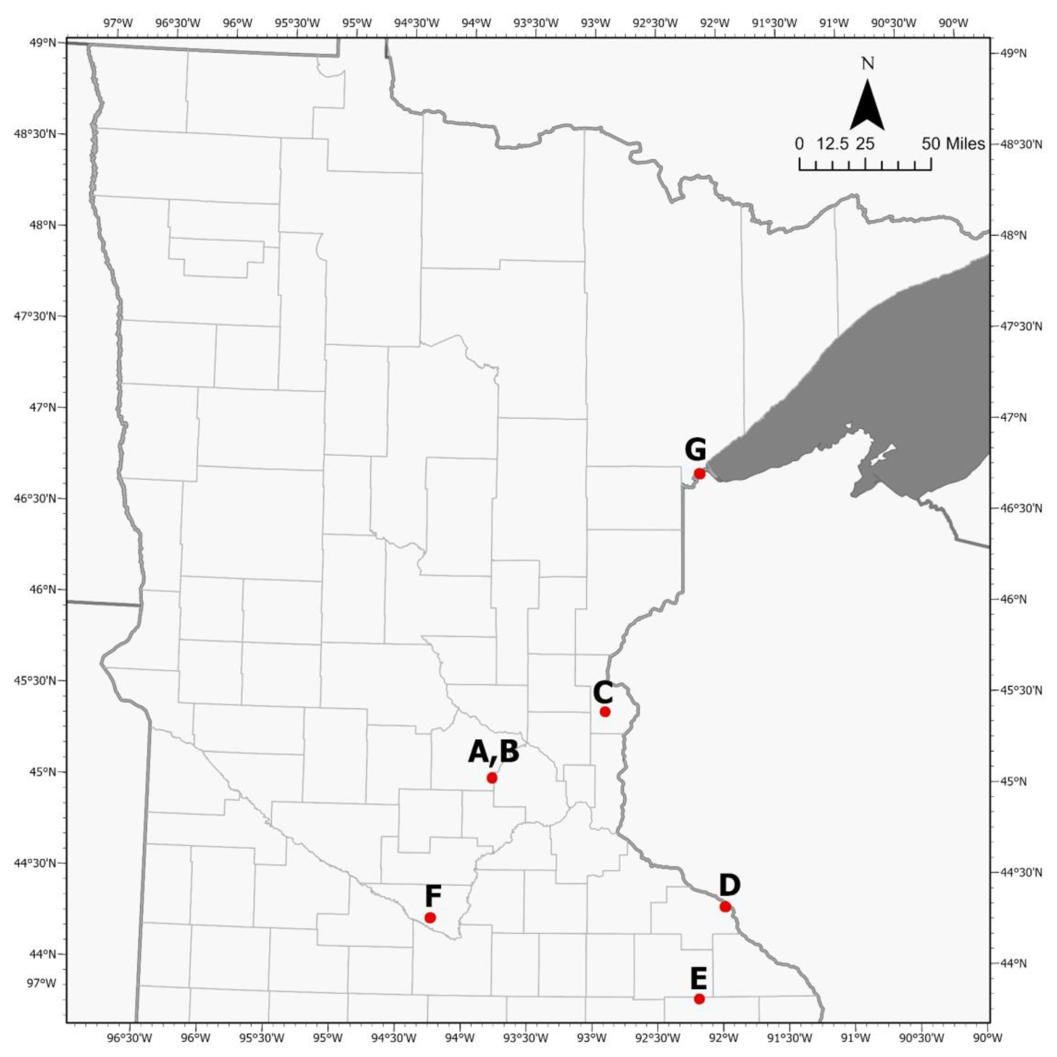
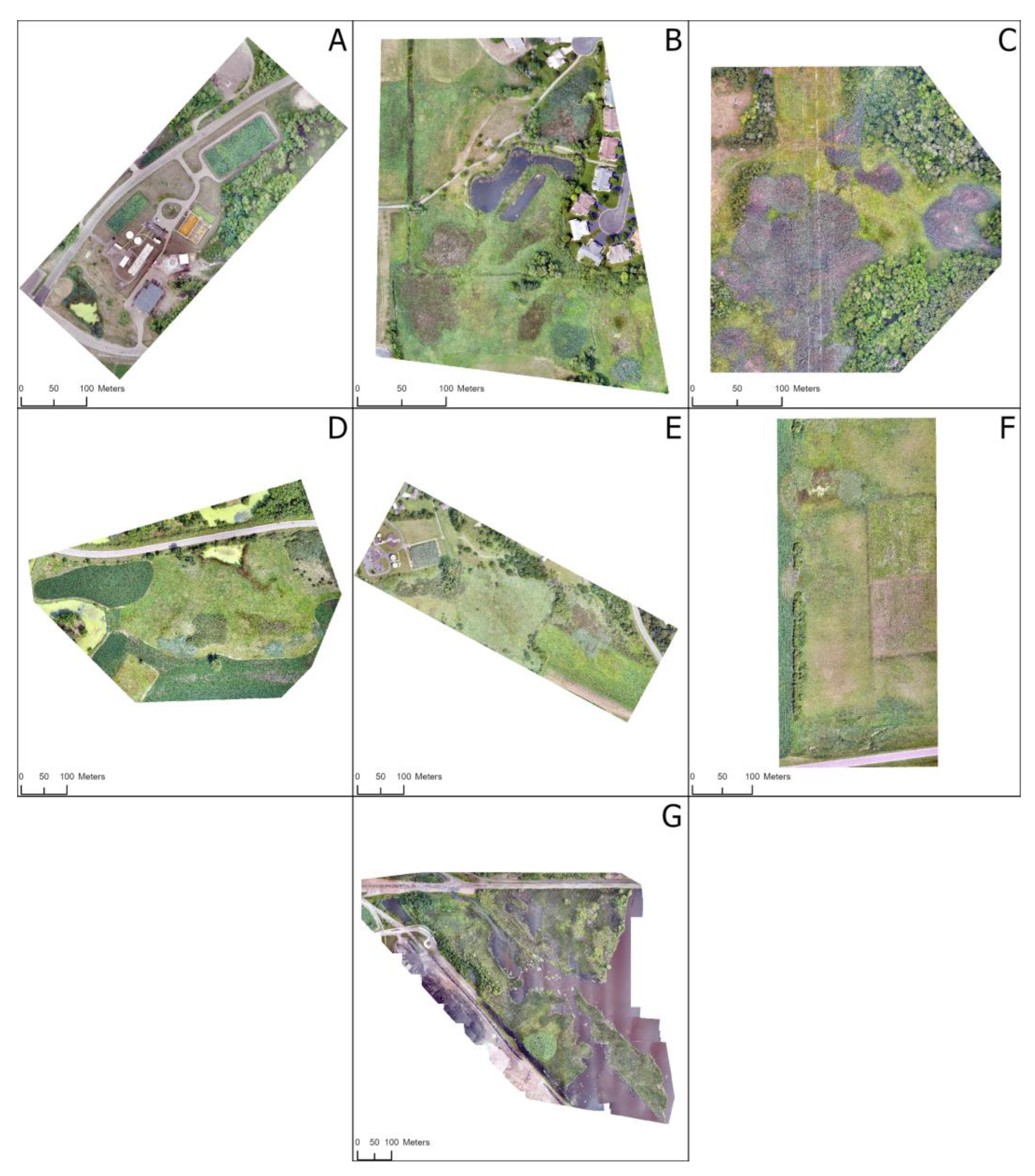
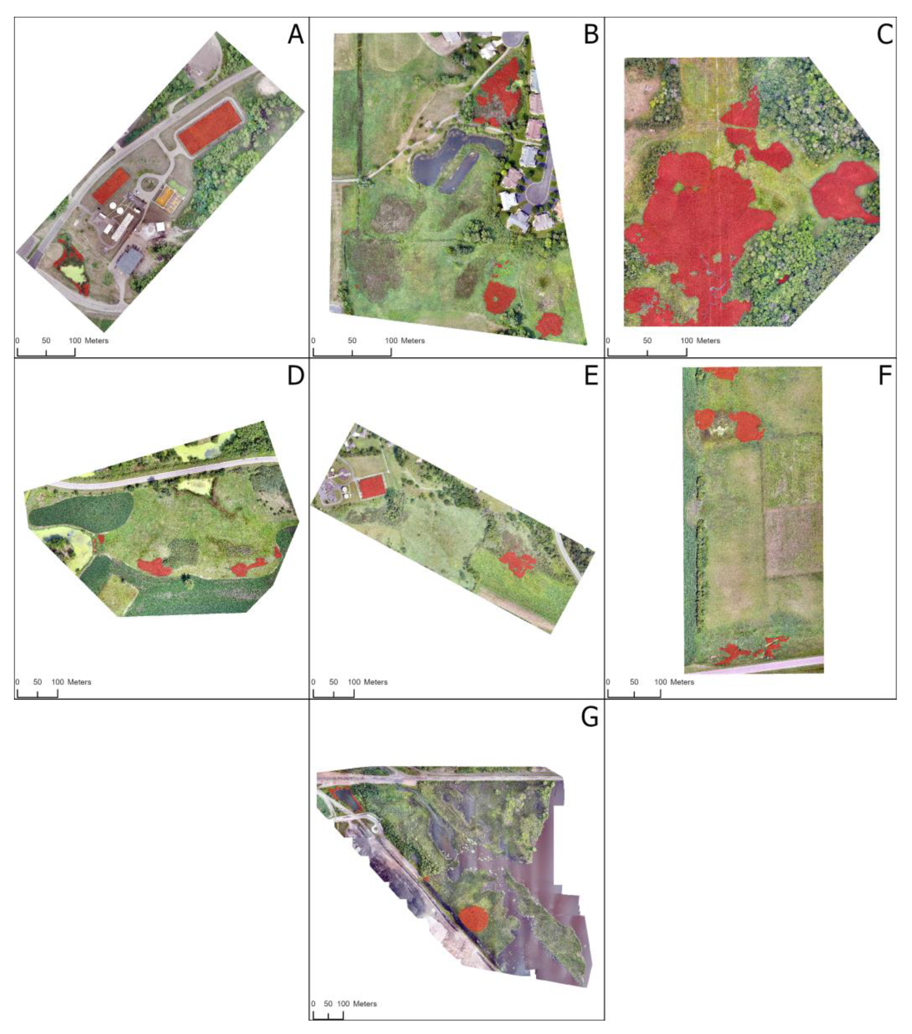
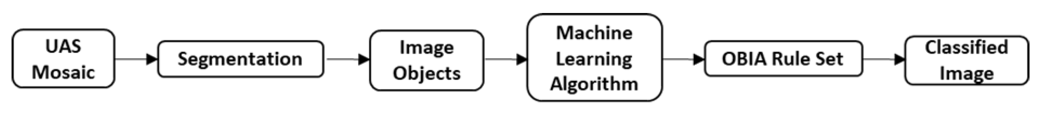
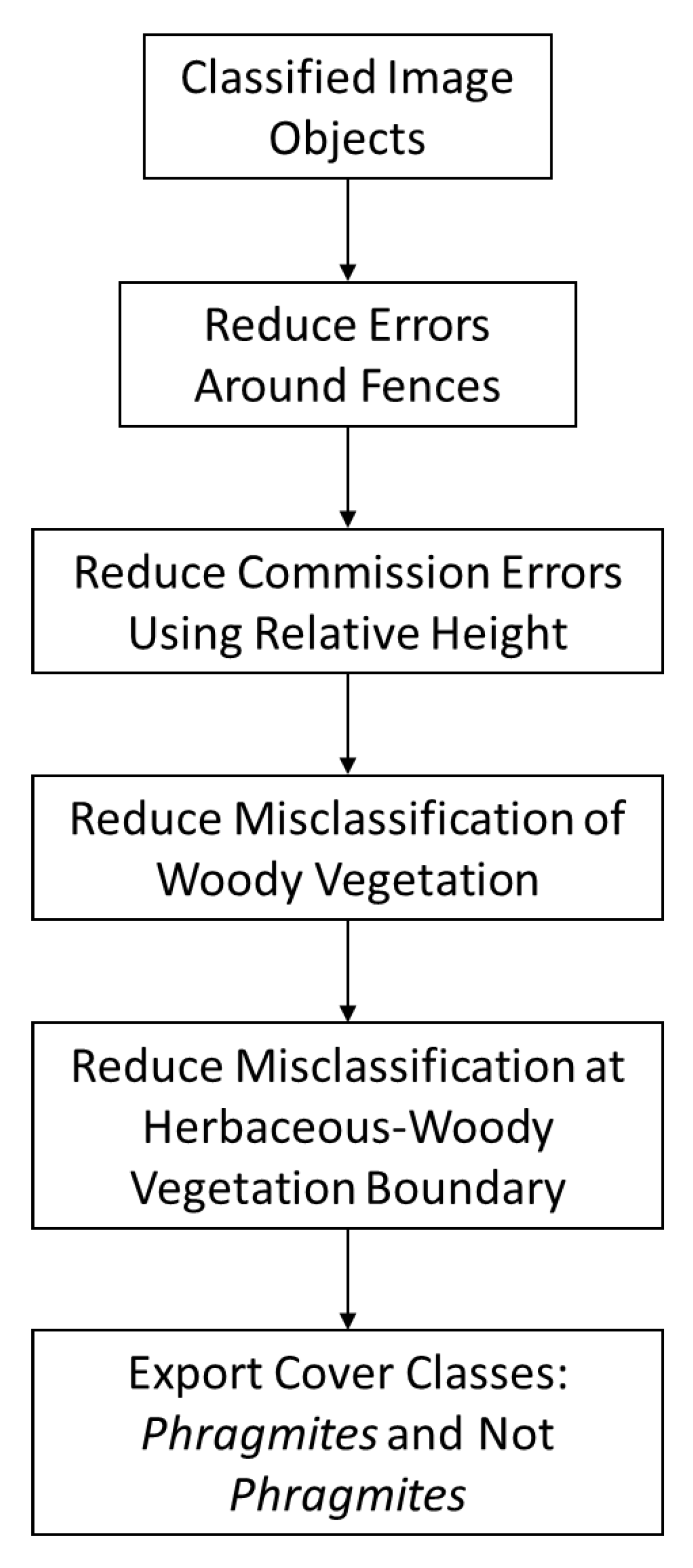
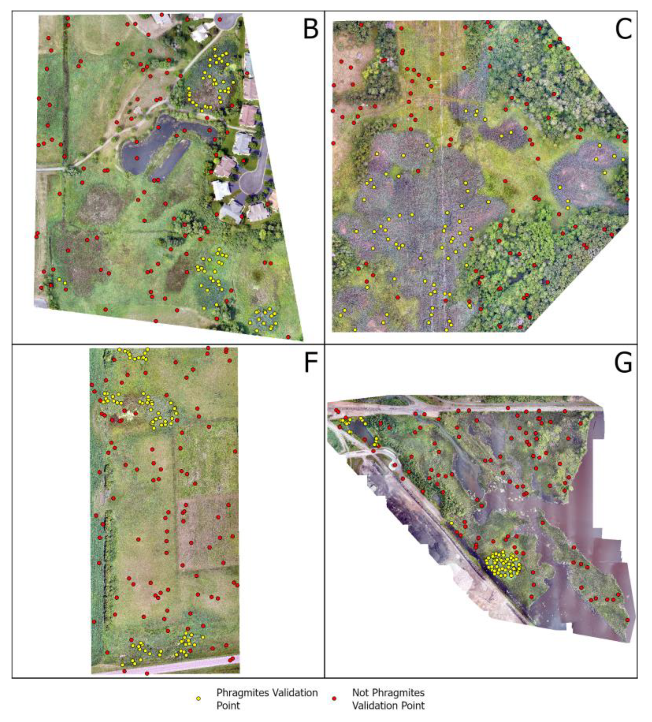
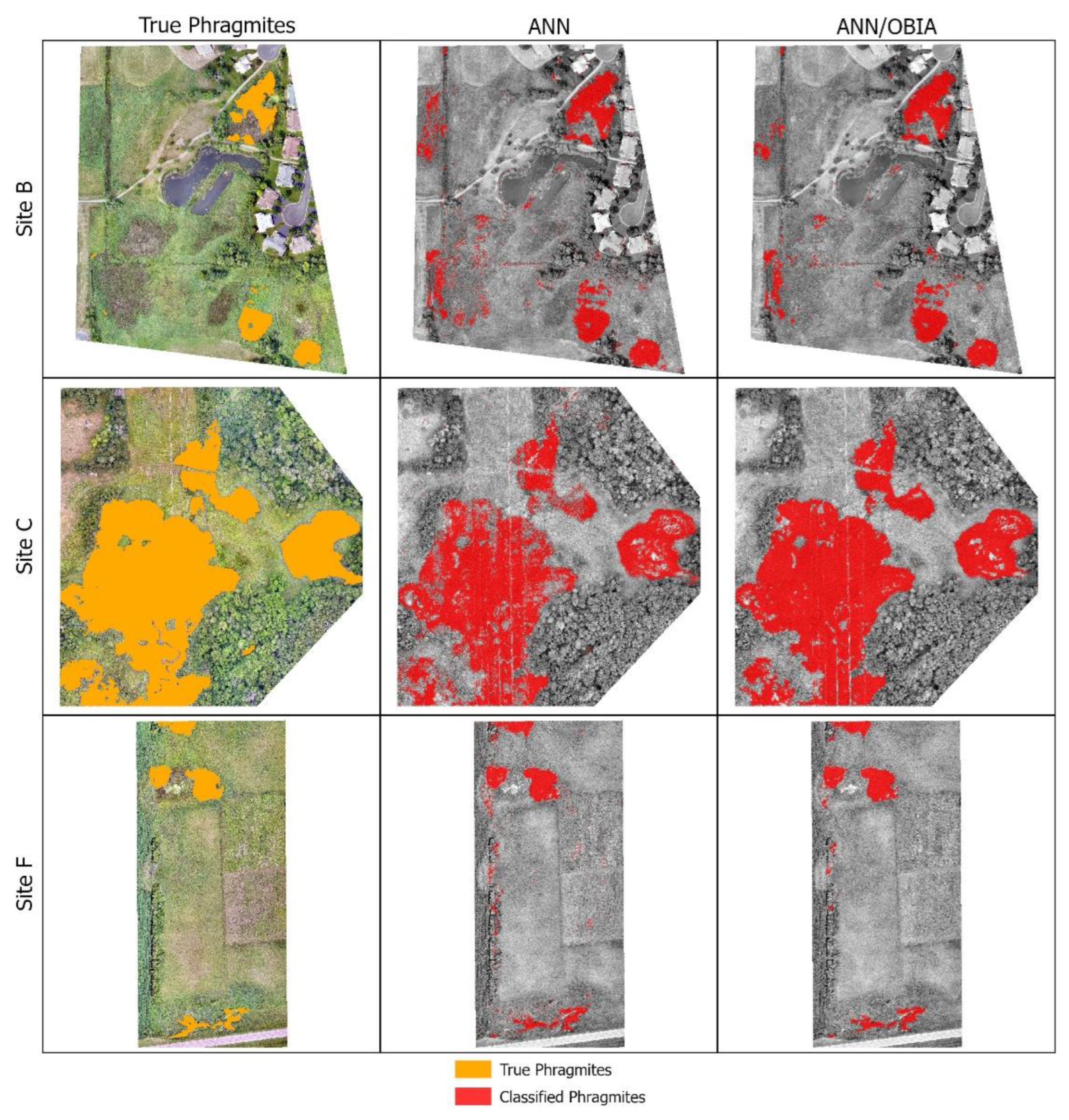
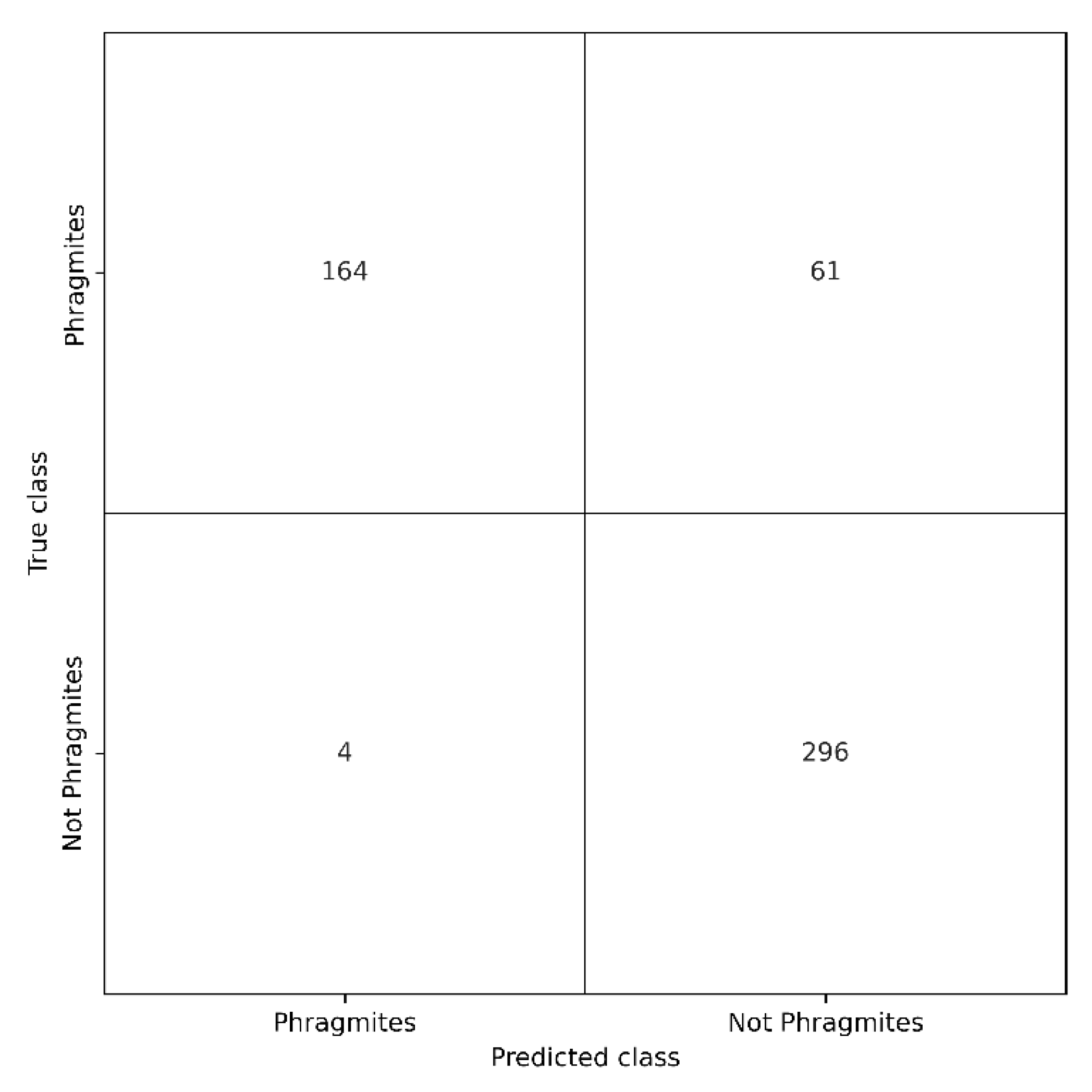
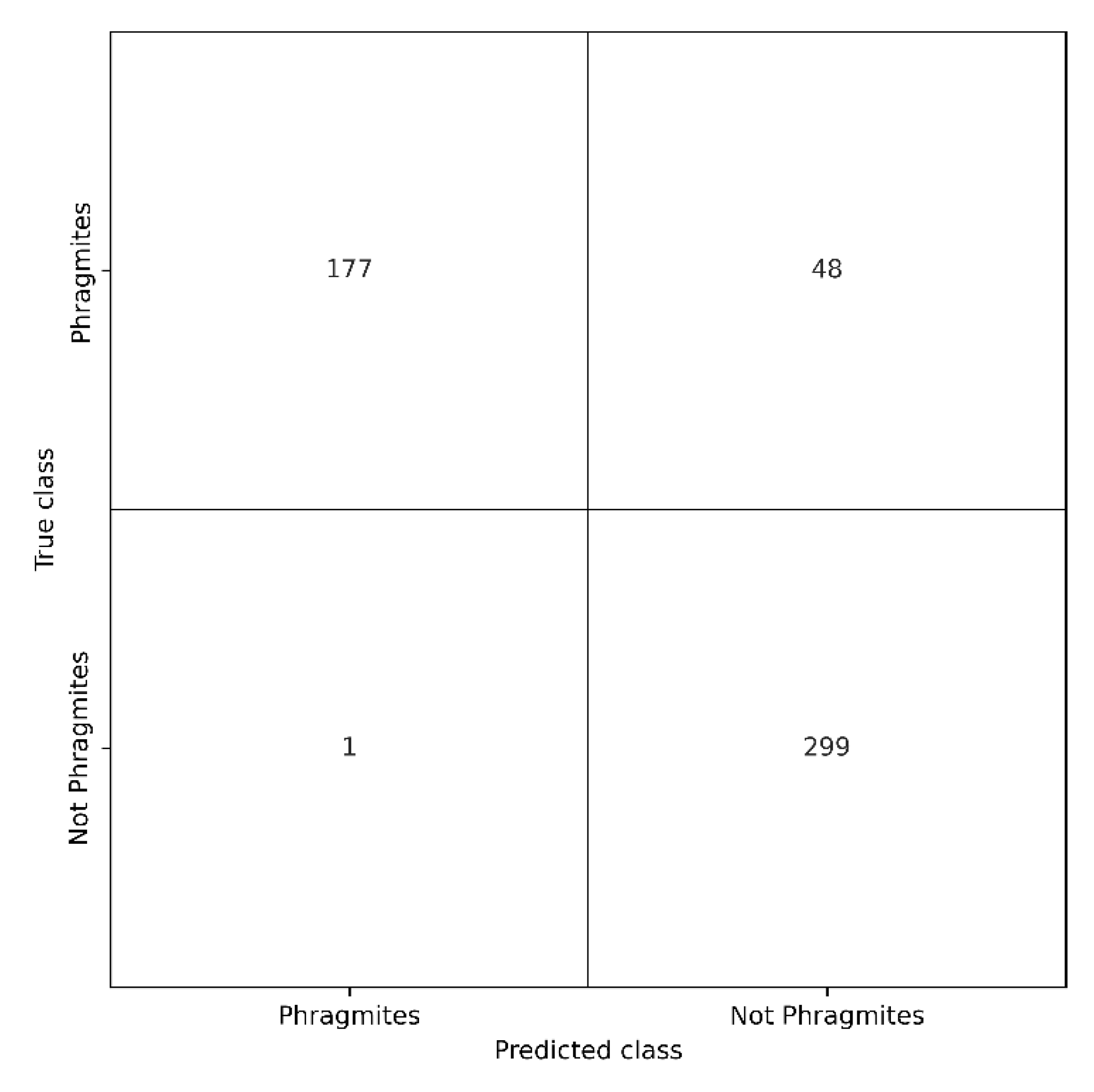
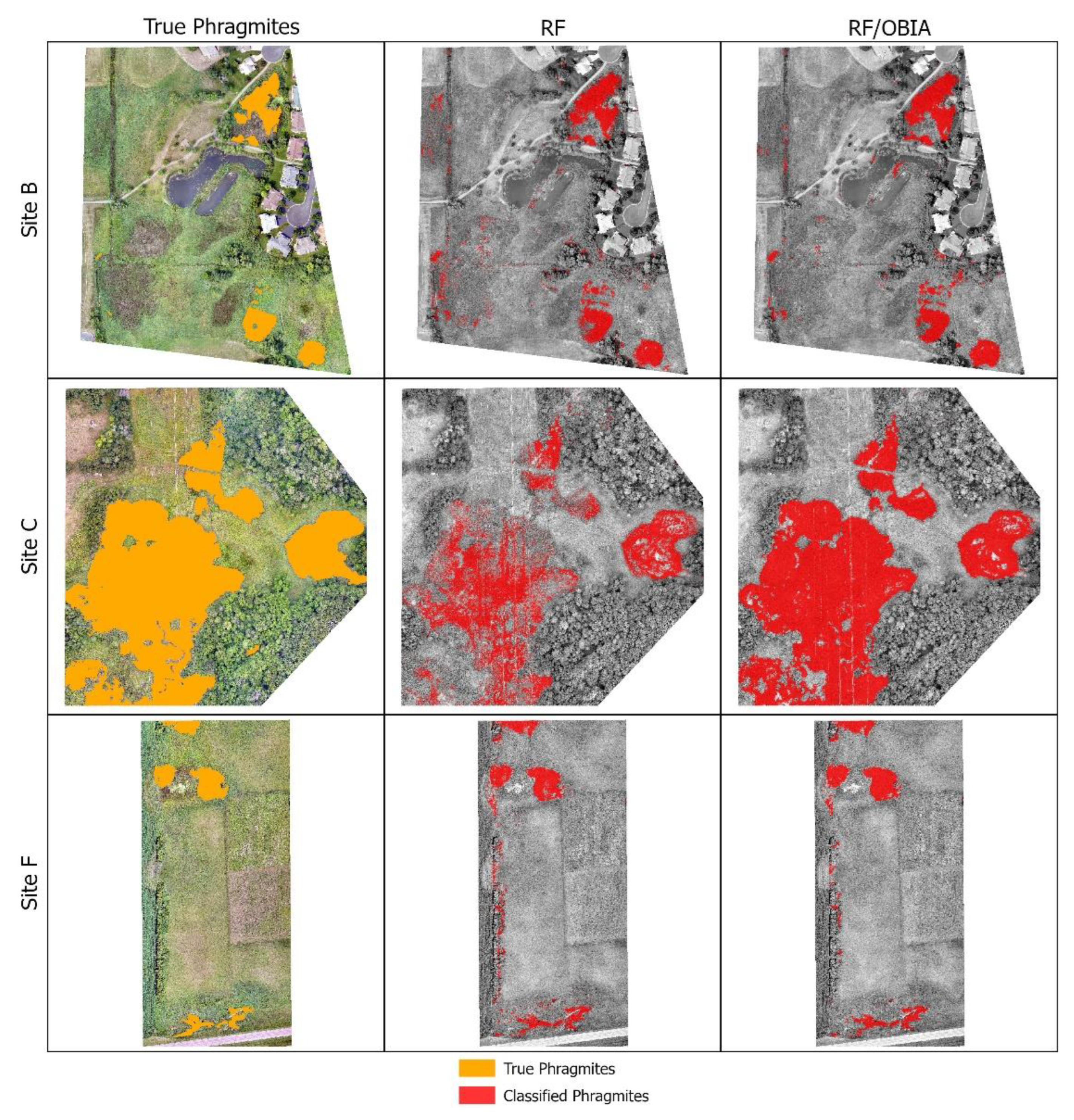
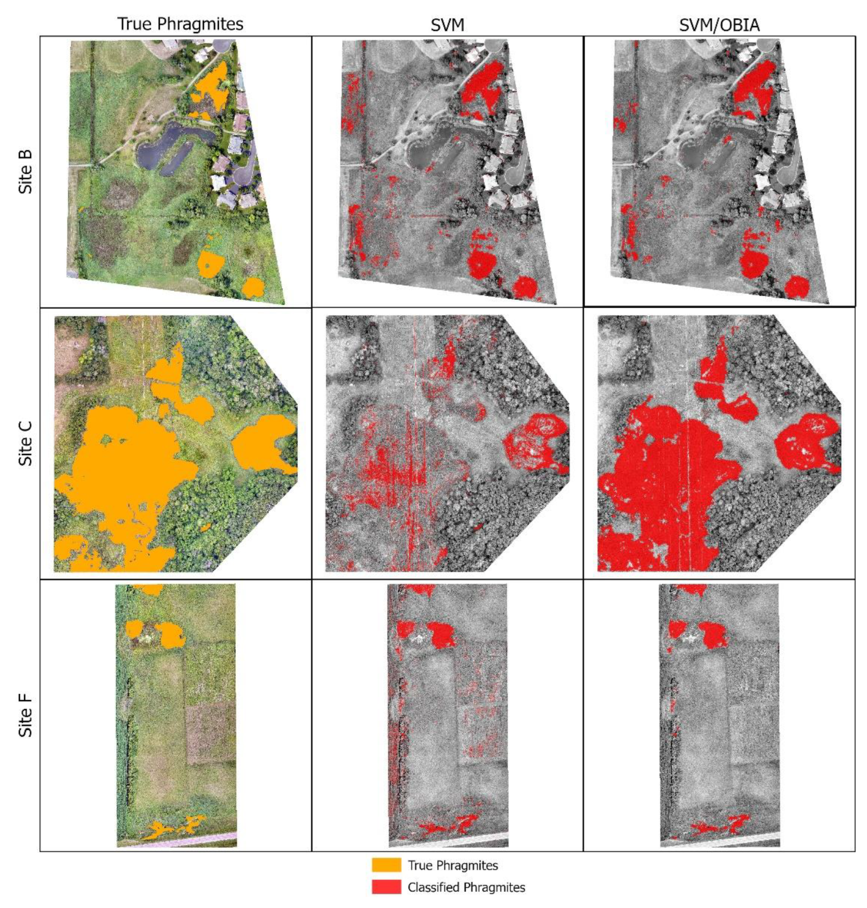
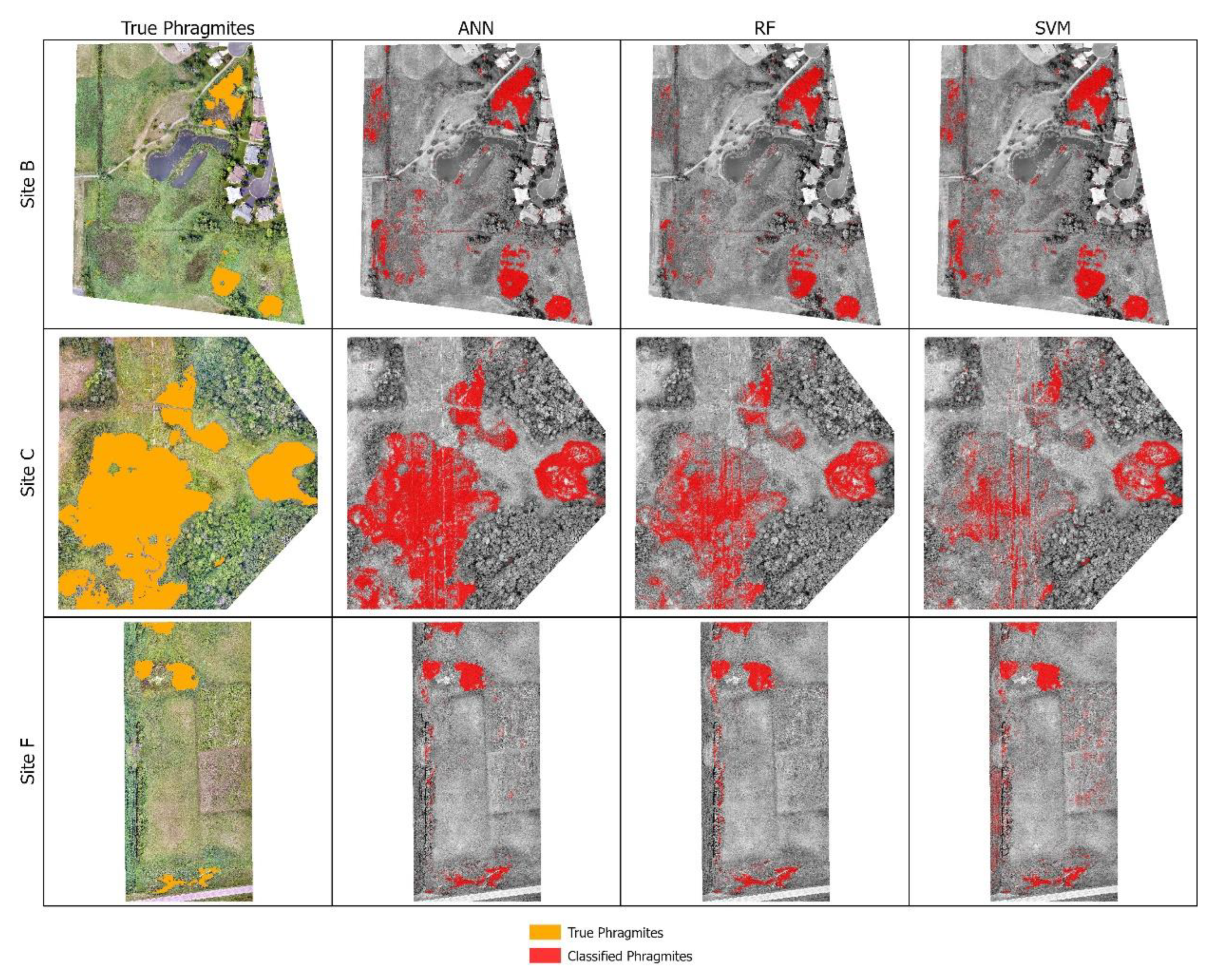
Table 1.
UAS collections at each study area. All imagery in 2021 was acquired at 121 m above ground level with 85% endlap and 70% sidelap. Grassy Point Park was collected in 2018 with 85% endlap and 65% sidelap.
Table 1.
UAS collections at each study area. All imagery in 2021 was acquired at 121 m above ground level with 85% endlap and 70% sidelap. Grassy Point Park was collected in 2018 with 85% endlap and 65% sidelap.
| Study Area | Collection Date | Acres | Resolution | Weather |
|---|---|---|---|---|
| Delano WWTF | 22 July 2021 | 26.6 | 1.65 cm | Overcast, light precipitation, and gusting winds |
| Delano City Park | 22 July 2021 | 27.1 | 1.67 cm | Overcast and gusting winds |
| Chisago City Property | 29 July 2021 | 24.4 | 1.61 cm | Hazy from wildfire smoke |
| Wabasha Property | 12 August 2021 | 28.7 | 1.66 cm | Clear skies and moderate wind |
| Chatfield WWTF | 3 August 2021 | 38.1 | 1.61 cm | Clear skies with light haze from wildfire smoke |
| Swan Lake WMA | 19 July 2021 | 38.2 | 1.68 cm | Mostly clear and light wind |
| Grassy Point Park | 10 August 2018 | 71 | 2.64 cm | Clear skies and minimal wind |
Table 2.
Lidar collection periods for each study area.
| Study Area | County | Collection Period |
|---|---|---|
| Delano WWTF | Wright | 23 April–28 May 2008 |
| Delano City Park | Wright | 23 April–28 May 2008 |
| Chisago City Property | Chisago | 18–28 April 2007 |
| Wabasha | Wabasha | 18–24 November 2008 |
| Chatfield WWTF | Olmsted | 18–24 November 2008 |
| Swan Lake WMA | Nicollet | 8 April–5 May; 2–19 November 2010 |
| Grassy Point Park | St. Louis | 29–31 October; 2 and 8 November 2012 |
Table 3.
Parameters values used for the random forest classifier algorithm in scikit-learn. All values are the default options except for the number of trees.
Table 3.
Parameters values used for the random forest classifier algorithm in scikit-learn. All values are the default options except for the number of trees.
| Parameter | Value |
|---|---|
| Number of Trees | 500 |
| Maximum Depth | None |
| Minimum Samples for Split | 2 |
| Minimum Samples for Leaf | 1 |
| Minimum Weighted Fraction for Leaf Node | 0 |
| Number of Features to Consider During Search for Best Split | |
| Maximum Number of Leaf Nodes | None |
| Minimum Decrease in Impurity to Induce Split | 0 |
Table 4.
Parameters values used for the support vector machine classifier algorithm in scikit-learn. All values are the default options except for C and gamma.
Table 4.
Parameters values used for the support vector machine classifier algorithm in scikit-learn. All values are the default options except for C and gamma.
| Parameter | Value |
|---|---|
| Kernel | Radial Basis Function |
| C | 2154.43 |
| Gamma | 0.1 |
| Use Shrinking Heuristic | True |
| Tolerance for Stopping Criterion | 0.001 |
| Maximum Iterations | No Limit |
| Decision Function Shape | One vs. Rest |
Table 5.
Parameters values used for the artificial neural network classifier algorithm in scikit-learn. All values are the default options except for the random state.
Table 5.
Parameters values used for the artificial neural network classifier algorithm in scikit-learn. All values are the default options except for the random state.
| Parameter | Value |
|---|---|
| Number of Hidden Layers | 1 |
| Neurons per Hidden Layer | 100 |
| Activation Function | Rectified Linear Unit (relu) |
| Optimizer | Adam |
| Learning Rate | 0.001 |
| Number of Epochs | 200 |
| Tolerance | 0.0001 |
| Random State | 1 |
Table 6.
Number of Phragmites polygons digitized and the total area in acres of Phragmites per study area.
Table 6.
Number of Phragmites polygons digitized and the total area in acres of Phragmites per study area.
| Study Area | Number of Phragmites Polygons | Total Area (Acres) |
|---|---|---|
| Delano WWTF | 11 | 1.76 |
| Wabasha | 6 | 0.63 |
| Chatfield WWTF | 9 | 1.38 |
Table 7.
Parameters exported from eCognition to be used in machine learning classifiers.
| Parameter | Source |
|---|---|
| Brightness | [70] |
| Edge Contrast of Blue Band (Window: 10) | [70] |
| Edge Contrast of Green Band (Window: 10) | [70] |
| Edge Contrast of nDSM (Window: 10) | [70] |
| Edge Contrast of Red Band (Window: 10) | [70] |
| Gray-Level Co-occurrence Matrix: Contrast | [69] |
| Gray-Level Co-occurrence Matrix: Homogeneity | [69] |
| Maximum Difference | [70] |
| Mean of Blue Band | |
| Mean of Green Band | |
| Mean of nDSM | |
| Mean of Red Band | |
| Mean Red-Blue Ratio | |
| Mean VARI | |
| Mean VDVI | |
| Standard Deviation of nDSM | |
| Standard Deviation of Red-Blue Ratio | |
| 25th Quantile of nDSM | |
| 90th Quantile of nDSM |
Table 8.
Number of training samples per cover class for each machine learning model.
| Cover Class | ||||||
|---|---|---|---|---|---|---|
| Model | Mowed Grass | Phragmites | Tree | Short Tree | Wetland | Agriculture |
| ANN | 9312 | 51,510 | 31,591 | 15,223 | 141,382 | 69,057 |
| RF | 9312 | 51,510 | 31,591 | 15,223 | 141,382 | 69,057 |
| SVM | 4656 | 5151 | 6318 | 7612 | 7069 | 6951 |
Table 9.
Validation points per cover class for each validation site. The total number of points randomly generated, the number manually verified through image interpretation, and the number selected from the verified points are provided.
Table 9.
Validation points per cover class for each validation site. The total number of points randomly generated, the number manually verified through image interpretation, and the number selected from the verified points are provided.
| Phragmites Class | Generated | Verified | Selected |
|---|---|---|---|
| Delano City Park | 150 | 115 | 75 |
| Chisago City Property | 150 | 146 | 75 |
| Swan Lake WMA | 150 | 88 | 75 |
| Grassy Point Park | 150 | 77 | 75 |
| Not Phragmites Class | Generated | Verified | Selected |
| Delano City Park | 200 | 185 | 100 |
| Chisago City Property | 200 | 123 | 100 |
| Swan Lake WMA | 200 | 191 | 100 |
| Grassy Point Park | 200 | 143 | 100 |
Table 10.
Validation assessment points for each of the three validation sites for the artificial neural network classification without the post-ML OBIA rule set.
Table 10.
Validation assessment points for each of the three validation sites for the artificial neural network classification without the post-ML OBIA rule set.
| Phragmites Class | Not Phragmites Class | |||
|---|---|---|---|---|
| Site | Correct | Incorrect | Correct | Incorrect |
| Delano City Park | 61 | 14 | 96 | 4 |
| Chisago City Property | 50 | 25 | 100 | 0 |
| Swan Lake WMA | 53 | 22 | 100 | 0 |
Table 11.
Errors of commission (EC), errors of omission (EO), and Matthews correlation coefficient (MCC) values for the artificial neural network classification without the post-ML OBIA rule set.
Table 11.
Errors of commission (EC), errors of omission (EO), and Matthews correlation coefficient (MCC) values for the artificial neural network classification without the post-ML OBIA rule set.
| Phragmites Class | Not Phragmites Class | ||||
|---|---|---|---|---|---|
| Site | EC | EO | EC | EO | MCC |
| Delano City Park | 6% | 19% | 13% | 4% | 0.79 |
| Chisago City Property | 0% | 33% | 20% | 0% | 0.73 |
| Swan Lake WMA | 0% | 29% | 18% | 0% | 0.76 |
| Combined | 2% | 27% | 17% | 1% | 0.76 |
Table 12.
Validation assessment points for each of the three validation sites for the artificial neural network classification with the post-ML OBIA rule set.
Table 12.
Validation assessment points for each of the three validation sites for the artificial neural network classification with the post-ML OBIA rule set.
| Phragmites Class | Not Phragmites Class | |||
|---|---|---|---|---|
| Site | Correct | Incorrect | Correct | Incorrect |
| Delano City Park | 63 | 12 | 99 | 1 |
| Chisago City Property | 61 | 14 | 100 | 0 |
| Swan Lake WMA | 53 | 22 | 100 | 0 |
Table 13.
Errors of commission (EC), errors of omission (EO), and Matthews correlation coefficient (MCC) values for the artificial neural network classification with the post-ML OBIA rule set.
Table 13.
Errors of commission (EC), errors of omission (EO), and Matthews correlation coefficient (MCC) values for the artificial neural network classification with the post-ML OBIA rule set.
| Phragmites Class | Not Phragmites Class | ||||
|---|---|---|---|---|---|
| Site | EC | EO | EC | EO | MCC |
| Delano City Park | 2% | 16% | 11% | 1% | 0.85 |
| Chisago City Property | 0% | 19% | 12% | 0% | 0.84 |
| Swan Lake WMA | 0% | 29% | 18% | 0% | 0.76 |
| Combined | 1% | 21% | 14% | 0% | 0.82 |
Table 14.
Validation assessment points for each of the three validation sites for the random forest classification without the post-ML OBIA rule set.
Table 14.
Validation assessment points for each of the three validation sites for the random forest classification without the post-ML OBIA rule set.
| Phragmites Class | Not Phragmites Class | |||
|---|---|---|---|---|
| Site | Correct | Incorrect | Correct | Incorrect |
| Delano City Park | 58 | 17 | 98 | 2 |
| Chisago City Property | 36 | 39 | 100 | 0 |
| Swan Lake WMA | 51 | 24 | 99 | 1 |
Table 15.
Errors of commission (EC), errors of omission (EO), and Matthews correlation coefficient (MCC) values for the random forest classification without the post-ML OBIA rule set.
Table 15.
Errors of commission (EC), errors of omission (EO), and Matthews correlation coefficient (MCC) values for the random forest classification without the post-ML OBIA rule set.
| Phragmites Class | Not Phragmites Class | ||||
|---|---|---|---|---|---|
| Site | EC | EO | EC | EO | MCC |
| Delano City Park | 3% | 23% | 15% | 2% | 0.79 |
| Chisago City Property | 0% | 52% | 28% | 0% | 0.59 |
| Swan Lake WMA | 2% | 32% | 20% | 1% | 0.73 |
| Combined | 2% | 36% | 21% | 1% | 0.7 |
Table 16.
Validation assessment points for each of the three validation sites for the random forest classification with the post-ML OBIA rule set.
Table 16.
Validation assessment points for each of the three validation sites for the random forest classification with the post-ML OBIA rule set.
| Phragmites Class | Not Phragmites Class | |||
|---|---|---|---|---|
| Site | Correct | Incorrect | Correct | Incorrect |
| Delano City Park | 61 | 14 | 100 | 0 |
| Chisago City Property | 67 | 8 | 99 | 1 |
| Swan Lake WMA | 54 | 21 | 99 | 1 |
Table 17.
Errors of commission (EC), errors of omission (EO), and Matthews correlation coefficient (MCC) values for the random forest classification with the post-ML OBIA rule set.
Table 17.
Errors of commission (EC), errors of omission (EO), and Matthews correlation coefficient (MCC) values for the random forest classification with the post-ML OBIA rule set.
| Phragmites Class | Not Phragmites Class | ||||
|---|---|---|---|---|---|
| Site | EC | EO | EC | EO | MCC |
| Delano City Park | 0% | 19% | 12% | 0% | 0.84 |
| Chisago City Property | 1% | 11% | 7% | 1% | 0.86 |
| Swan Lake WMA | 2% | 28% | 17% | 1% | 0.76 |
| Combined | 1% | 19% | 1% | 13% | 0.83 |
Table 18.
Validation assessment points for each of the three validation sites for the support vector machine classification without the post-ML OBIA rule set.
Table 18.
Validation assessment points for each of the three validation sites for the support vector machine classification without the post-ML OBIA rule set.
| Phragmites Class | Not Phragmites Class | |||
|---|---|---|---|---|
| Site | Correct | Incorrect | Correct | Incorrect |
| Delano City Park | 58 | 17 | 97 | 3 |
| Chisago City Property | 20 | 55 | 98 | 2 |
| Swan Lake WMA | 50 | 25 | 97 | 3 |
Table 19.
Errors of commission (EC), errors of omission (EO), and Matthews correlation coefficient (MCC) values for the support vector machine classification without the post-ML OBIA rule set.
Table 19.
Errors of commission (EC), errors of omission (EO), and Matthews correlation coefficient (MCC) values for the support vector machine classification without the post-ML OBIA rule set.
| Phragmites Class | Not Phragmites Class | ||||
|---|---|---|---|---|---|
| Site | EC | EO | EC | EO | MCC |
| Delano City Park | 5% | 23% | 15% | 3% | 0.77 |
| Chisago City Property | 9% | 73% | 36% | 2% | 0.37 |
| Swan Lake WMA | 6% | 33% | 20% | 3% | 0.69 |
| Combined | 6% | 43% | 25% | 3% | 0.61 |
Table 20.
Validation assessment points for each of the three validation sites for the support vector machine classification with the post-ML OBIA rule set.
Table 20.
Validation assessment points for each of the three validation sites for the support vector machine classification with the post-ML OBIA rule set.
| Phragmites Class | Not Phragmites Class | |||
|---|---|---|---|---|
| Site | Correct | Incorrect | Correct | Incorrect |
| Delano City Park | 64 | 11 | 99 | 1 |
| Chisago City Property | 69 | 6 | 98 | 2 |
| Swan Lake WMA | 50 | 25 | 99 | 1 |
Table 21.
Errors of commission (EC), errors of omission (EO), and Matthews correlation coefficient (MCC) values for the support vector machine classification with the post-ML OBIA rule set.
Table 21.
Errors of commission (EC), errors of omission (EO), and Matthews correlation coefficient (MCC) values for the support vector machine classification with the post-ML OBIA rule set.
| Phragmites Class | Not Phragmites Class | ||||
|---|---|---|---|---|---|
| Site | EC | EO | EC | EO | MCC |
| Delano City Park | 2% | 15% | 10% | 1% | 0.86 |
| Chisago City Property | 3% | 8% | 6% | 2% | 0.91 |
| Swan Lake WMA | 2% | 33% | 20% | 1% | 0.72 |
| Combined | 2% | 19% | 12% | 9% | 0.83 |
Table 22.
Validation assessment points for Grassy Point Park for each of the classification methods.
Table 22.
Validation assessment points for Grassy Point Park for each of the classification methods.
| Phragmites Class | Not Phragmites Class | |||
|---|---|---|---|---|
| Method | Correct | Incorrect | Correct | Incorrect |
| ANN | 18 | 57 | 73 | 27 |
| ANN/OBIA | 73 | 2 | 89 | 11 |
| RF | 53 | 22 | 71 | 29 |
| RF/OBIA | 73 | 2 | 91 | 9 |
| SVM | 34 | 41 | 78 | 22 |
| SVM/OBIA | 69 | 6 | 89 | 11 |
Table 23.
Errors of commission (EC), errors of omission (EO), and F1 scores for Grassy Point Park for each of the classification methods.
Table 23.
Errors of commission (EC), errors of omission (EO), and F1 scores for Grassy Point Park for each of the classification methods.
| Phragmites Class | Not Phragmites Class | ||||
|---|---|---|---|---|---|
| Site | EC | EO | EC | EO | F1 Score |
| ANN | 60% | 76% | 44% | 27% | −0.03 |
| ANN/OBIA | 13% | 3% | 2% | 11% | 0.86 |
| RF | 35% | 29% | 24% | 29% | 0.7 |
| RF/OBIA | 11% | 3% | 2% | 9% | 0.88 |
| SVM | 39% | 55% | 34% | 22% | 0.25 |
| SVM/OBIA | 14% | 8% | 6% | 11% | 0.8 |
Disclaimer/Publisher’s Note: The statements, opinions and data contained in all publications are solely those of the individual author(s) and contributor(s) and not of MDPI and/or the editor(s). MDPI and/or the editor(s) disclaim responsibility for any injury to people or property resulting from any ideas, methods, instructions or products referred to in the content. |
© 2023 by the authors. Licensee MDPI, Basel, Switzerland. This article is an open access article distributed under the terms and conditions of the Creative Commons Attribution (CC BY) license (https://creativecommons.org/licenses/by/4.0/).
Share and Cite
MDPI and ACS Style
Anderson, C.J.; Heins, D.; Pelletier, K.C.; Knight, J.F. Improving Machine Learning Classifications of Phragmites australis Using Object-Based Image Analysis. Remote Sens. 2023, 15, 989. https://doi.org/10.3390/rs15040989
AMA Style
Anderson CJ, Heins D, Pelletier KC, Knight JF. Improving Machine Learning Classifications of Phragmites australis Using Object-Based Image Analysis. Remote Sensing. 2023; 15(4):989. https://doi.org/10.3390/rs15040989
Chicago/Turabian StyleAnderson, Connor J., Daniel Heins, Keith C. Pelletier, and Joseph F. Knight. 2023. "Improving Machine Learning Classifications of Phragmites australis Using Object-Based Image Analysis" Remote Sensing 15, no. 4: 989. https://doi.org/10.3390/rs15040989
Note that from the first issue of 2016, this journal uses article numbers instead of page numbers. See further details here.