
Evaluation of InSAR Tropospheric Delay Correction Methods in a Low-Latitude Alpine Canyon Region


Abstract
:1. Introduction
2. Materials and Methods
2.1. InSAR Tropospheric Delay
2.1.1. Linear Correction Method
2.1.2. Generic Atmospheric Correction Online Service for InSAR (GACOS) Correction Method
2.1.3. High-Resolution Numerical Atmospheric Model (ERA5) Correction Method
2.2. Study Area and Data Processing
2.2.1. Overview of the Study Area and Data Sources
2.2.2. Research Method
3. Results
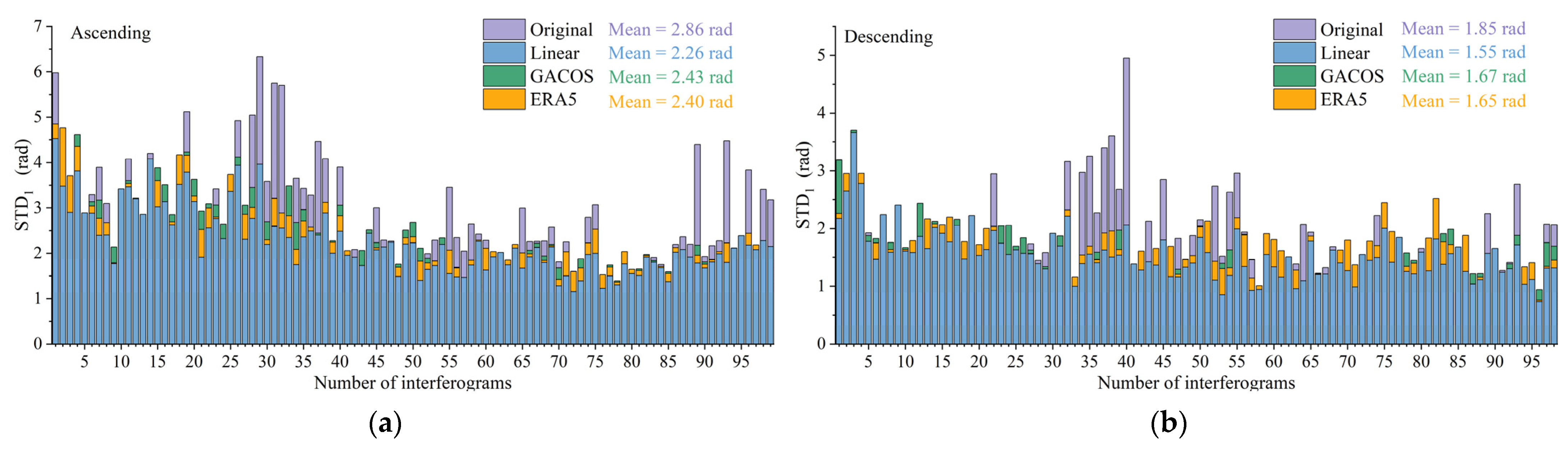
3.1. STD Evaluation
3.2. Semi-Variance Function Evaluation
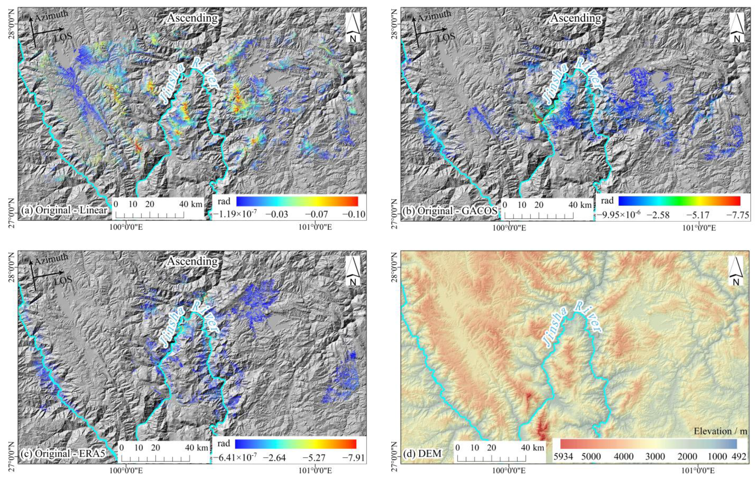
3.3. Elevation Correlation Evaluation
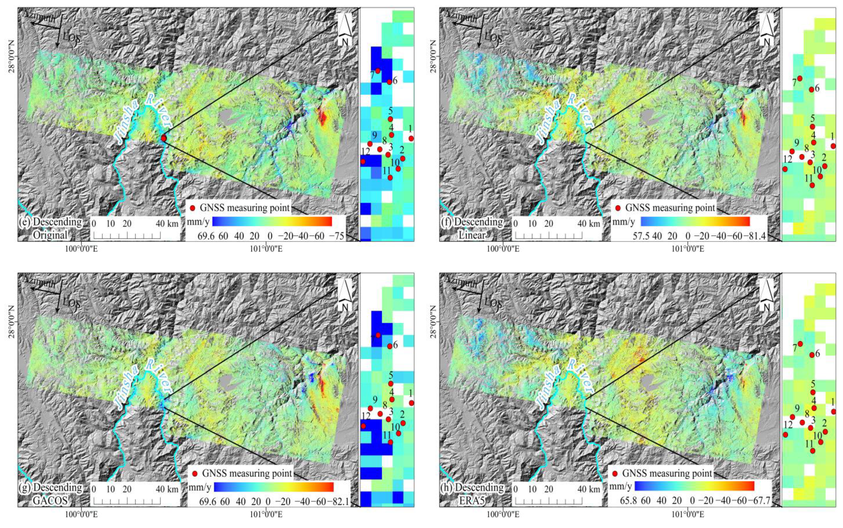
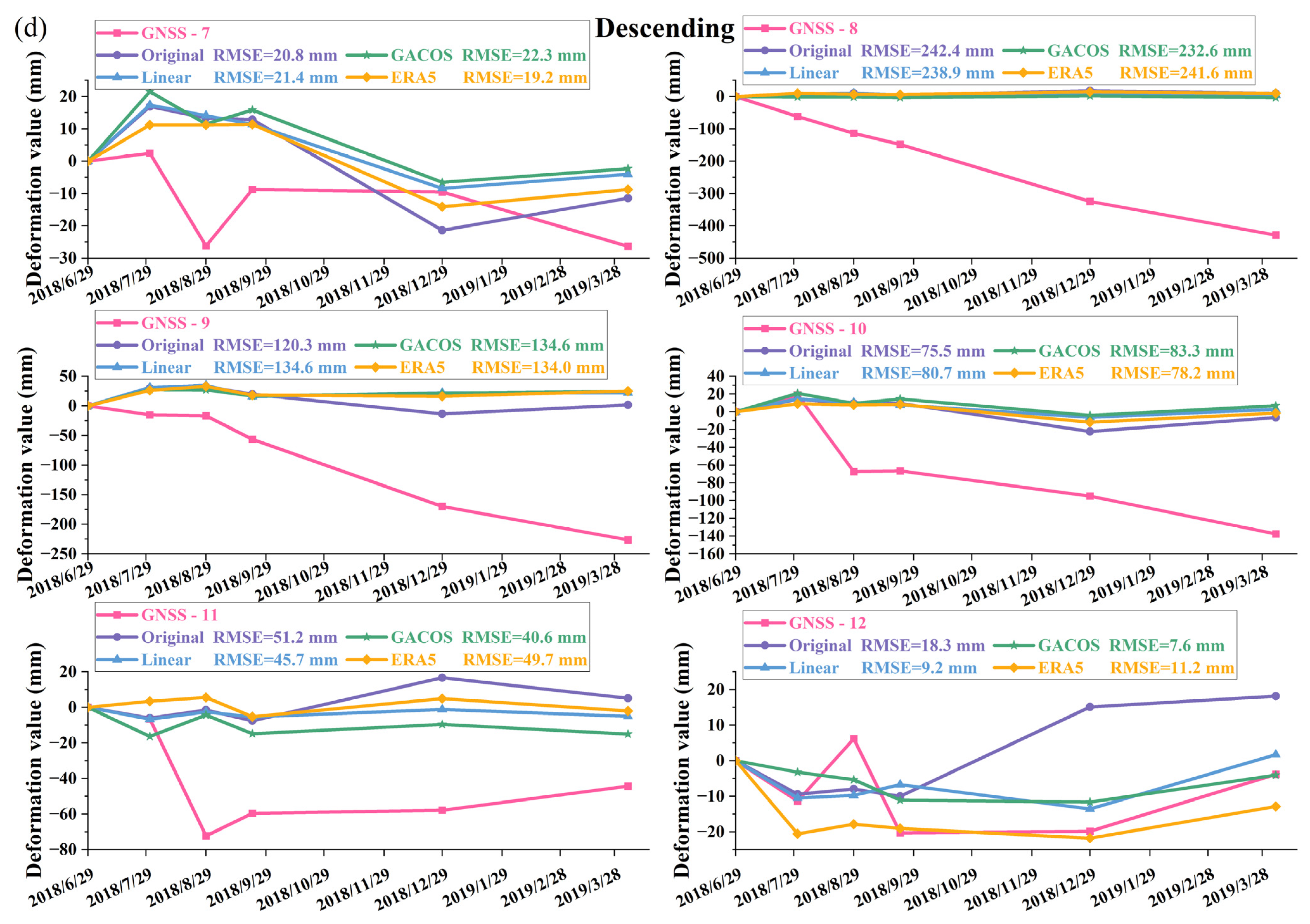
3.4. GNSS Station Deformation Monitoring and Evaluation
4. Discussion
5. Conclusions
Author Contributions
Funding
Data Availability Statement
Acknowledgments
Conflicts of Interest
References
- Li, Z.; Zhu, W.; Yu, C.; Zhang, Q.; Zhang, C.; Liu, Z.; Zhang, X.; Chen, B.; Du, J.; Song, C.; et al. Interferometric synthetic aperture radar for deformation mapping: Opportunities, challenges and the outlook. Acta Geod. Cartogr. Sinica. 2022, 51, 1485–1519. [Google Scholar] [CrossRef]
- Bekaert, D.; Walters, R.; Wright, T.; Hooper, A.; Parker, D. Statistical comparison of InSAR tropospheric correction techniques. Remote Sens. Environ. 2015, 170, 40–47. [Google Scholar] [CrossRef]
- Li, P.; Gao, M.; Li, Z.; Wang, H. Evaluation of Wide-Swath InSAR Tropospheric Delay Estimation Methods over the Altyn Tagh Fault. Geomat. Inf. Sci. Wuhan Univ. 2020, 45, 879–887. [Google Scholar] [CrossRef]
- Zebker, H.A.; Rosen, P.A.; Hensley, S. Atmospheric effects in interferometric synthetic aperture radar surface deformation and topographic maps. J. Geophys. Res. Solid Earth 1997, 102, 7547–7563. [Google Scholar] [CrossRef]
- Murray, K.; Bekaert, D.; Lohman, R. Tropospheric corrections for InSAR: Statistical assessments and applications to the Central United States and Mexico. Remote Sens. Environ. 2019, 232, 111326. [Google Scholar] [CrossRef]
- Li, Z.; Muller, J.-P.; Cross, P.; Fielding, E. Interferometric synthetic aperture radar (InSAR) atmospheric correction: GPS, Moderate Resolution Imaging Spectroradiometer (MODIS), and InSAR integration. J. Geophys. Res. Atmos. 2005, 110, B03410. [Google Scholar] [CrossRef]
- Bekaert, D.P.S.; Hooper, A.; Wright, T.J. Reassessing the 2006 Guerrero slow-slip event, Mexico: Implications for large earthquakes in the Guerrero Gap. J. Geophys. Res. Solid Earth 2015, 120, 1357–1375. [Google Scholar] [CrossRef]
- Song, X.; Li, D.; Liao, M.; Cheng, L. A Method to Correct Tropospheric Delay in SAR Interferometry from GPS Observations. Geomat. Inf. Sci. Wuhan Univ. 2008, 33, 233–236. [Google Scholar]
- Zhang, Z.; Lou, Y.; Zhang, W.; Wang, H.; Zhou, Y.; Bai, J. Assessment of ERA-Interim and ERA5 reanalysis data on atmospheric corrections for InSAR. Int. J. Appl. Earth Obs. Geoinf. 2022, 111, 102822. [Google Scholar] [CrossRef]
- Xiao, R.; Yu, C.; Li, Z.; He, X. Statistical assessment metrics for InSAR atmospheric correction: Applications to generic atmospheric correction online service for InSAR (GACOS) in Eastern China. Int. J. Appl. Earth Obs. Geoinf. 2020, 96, 102289. [Google Scholar] [CrossRef]
- Ghosh, B.; Haghighi, M.H.; Motagh, M.; Maghsudi, S. Using generative adversarial networks for extraction of insar signals from large-scale Sentinel-1 interferograms by improving tropospheric noise correction. ISPRS Ann. Photogramm. Remote Sens. Spat. Inf. Sci. 2021, V-3-2021, 57–64. [Google Scholar] [CrossRef]
- Liu, S.; Hanssen, R.; Mika, A. On the Value of High-Resolution Weather Models for Atmospheric Mitigation in SAR Interferometry. In Proceedings of the Geoscience and Remote Sensing Symposium, Cape Town, South Africa, 12–17 July 2009. [Google Scholar] [CrossRef]
- Smith, E.; Weintraub, S. The Constants in the Equation for Atmospheric Refractive Index at Radio Frequencies. Proc. IRE. 1953, 50, 1035–1037. [Google Scholar] [CrossRef]
- Doin, M.-P.; Lasserre, C.; Peltzer, G.; Cavalié, O.; Doubre, C. Corrections of stratified tropospheric delays in SAR interferometry: Validation with global atmospheric models. J. Appl. Geophys. 2009, 69, 35–50. [Google Scholar] [CrossRef]
- Lin, Y.-N.N.; Simons, M.; Hetland, E.A.; Muse, P.; DiCaprio, C. A multiscale approach to estimating topographically correlated propagation delays in radar interferograms. Geochem. Geophys. Geosyst. 2010, 11, Q09002. [Google Scholar] [CrossRef]
- Yu, C.; Li, Z.; Bai, L.; Muller, J.; Zhang, J.; Zeng, Q. Successful Applications of Generic Atmospheric Correction Online Service for InSAR (GACOS) to the Reduction of Atmospheric Effects on InSAR Observations. J. Geod. Geoinf. Sci. 2021, 4, 109–115. [Google Scholar] [CrossRef]
- Yu, C.; Penna, N.T.; Li, Z. Generation of real-time mode high-resolution water vapor fields from GPS observations. J. Geophys. Res. Atmos. 2017, 122, 2008–2025. [Google Scholar] [CrossRef]
- Yu, C.; Li, Z.; Penna, N.T.; Crippa, P. Generic Atmospheric Correction Model for Interferometric Synthetic Aperture Radar Observations. J. Geophys. Res. Solid Earth 2018, 123, 9202–9222. [Google Scholar] [CrossRef]
- Hersbach, H.; Bell, B.; Berrisford, P.; Hirahara, S.; Horanyi, A.; Muñoz-Sabater, J.; Nicolas, J.; Peubey, C.; Radu, R.; Schepers, D.; et al. The ERA5 global reanalysis. Q. J. R. Meteorol. Soc. 2020, 146, 1999–2049. [Google Scholar] [CrossRef]
- Li, Y.; Zuo, X.; Zhu, D.; Wu, W.; Yang, X.; Guo, S.; Shi, C.; Huang, C.; Li, F.; Liu, X. Identification and Analysis of Landslides in the Ahai Reservoir Area of the Jinsha River Basin Using a Combination of DS-InSAR, Optical Images, and Field Surveys. Remote Sens. 2022, 14, 6274. [Google Scholar] [CrossRef]
- Yin, G.; Wei, C.; Wang, D.; Du, J.; Wang, L.; Cheng, L.; Yuan, R.; Wang, X.; Liu, C. The multiple formation mechanism of the flu-lacustrine sediment in the southeast Tibetan Plateau: An example from the middle Jinsha River. Quat. Sci. 2022, 42, 797–808. [Google Scholar] [CrossRef]
- Berardino, P.; Fornaro, G.; Lanari, R.; Sansosti, E. A new algorithm for surface deformation monitoring based on small baseline differential SAR interferograms. IEEE Trans. Geosci. Remote Sens. 2002, 40, 2375–2383. [Google Scholar] [CrossRef]
- Liu, G.; Chen, Q.; Luo, X.; Cai, G. Principle and Application of InSAR; Science Press: Beijing, China, 2019; p. 70. [Google Scholar]
- Jolivet, R.; Agram, P.S.; Lin, N.Y.; Simons, M.; Doin, M.; Peltzer, G.; Li, Z. Improving InSAR geodesy using Global Atmospheric Models. J. Geophys. Res. Solid Earth 2014, 119, 2324–2341. [Google Scholar] [CrossRef]
- T/CAGHP 013-2018; Technical Guide for InSAR Monitoring of Geological Hazards (Trial). Available online: https://max.book118.com/html/2021/0113/6033010151003050.shtm (accessed on 1 September 2022).
- Tang, W. InSAR Tropospheric Delay Correction Using Atmospheric Reanalysis and Water Vapor Mapping. Ph.D. Thesis, Wuhan University, Wuhan, China, May 2017. [Google Scholar]
- Zhao, S. Aviation Meteorology; China Meteorological Press: Beijing, China, 1994; p. 7. [Google Scholar]
- Yan, H.; Dai, W.; Liu, H.; Gao, H.; Neely, W.R.; Xu, W. Fusion of Spatially Heterogeneous GNSS and InSAR Deformation Data Using a Multiresolution Segmentation Algorithm and Its Application in the Inversion of Slip Distribution. Remote Sens. 2022, 14, 3293. [Google Scholar] [CrossRef]
- GB/T 26424-2010; Technical Specification for Forest resources Planning, Design and Investigation. Available online: https://www.doc88.com/p-2095374604208.html (accessed on 3 February 2023).
- GB/T 38590-2020; Technical Specification for Continuous Inventory of Forest Resources. Available online: https://www.doc88.com/p-70159494801114.html (accessed on 3 February 2023).
- Zhu, J.; Li, Y.; Wang, T.; Chang, Z.; Yu, W.; Han, Y.; Wang, Y.; Liu, Y. An Improved Atmospheric Phase Delay Correction Method in Spaceborne Repeat-Track InSAR Monitoring. J. Geod. Geodyn. 2020, 40, 1164–1169. [Google Scholar] [CrossRef]
- Auslander, M.; Nevo, E.; Inbar, M. The effects of slope orientation on plant growth, developmental instability and susceptibility to herbivores. J. Arid. Environ. 2003, 55, 405–416. [Google Scholar] [CrossRef]
- Shen, L.; Hooper, A.; Elliott, J. A Spatially Varying Scaling Method for InSAR Tropospheric Corrections Using a High-Resolution Weather Model. J. Geophys. Res. Solid Earth 2019, 124, 4051–4068. [Google Scholar] [CrossRef] [Green Version]


| Tracks | Number of Images | Time Coverage | Beam Mode | Number of Initial Interferograms | Number of Final Interferograms |
|---|---|---|---|---|---|
| Ascending | 24 | 2018/06/17–2019/04/01 | IW | 113 | 99 |
| Descending | 24 | 2018/06/19–2019/04/03 | IW | 112 | 98 |
| Track | Evaluation Indicators | Original | Linear | GACOS | ERA5 |
|---|---|---|---|---|---|
| Ascending | Average of standard deviation of interference phase of all IFGs (Aver)/rad * | 2.86 | 2.26 | 2.43 | 2.40 |
| Rate of change | - | −20.98% | −15.03% | −16.08% | |
| Descending | Average of standard deviation of interference phase of all IFGs (Aver)/rad | 1.85 | 1.55 | 1.67 | 1.65 |
| Rate of change | - | −16.22% | −9.73% | −10.81% |
| Track | Evaluation Indicators | Linear | GACOS | ERA5 |
|---|---|---|---|---|
| Ascending | Number of IFGs increased/decreased by STD1 | +14/−85 1 | +29/−70 | +24/−75 |
| Rate of change of the average value of STD1 | +2.9%/−20.79% 2 | +8.97%/−19.62% | +7.14%/−18.69% | |
| Increase/Decrease of the average value of STD1 | +0.07/−0.72 rad 3 | +0.21/−0.70 rad | +0.17/−0.67 rad | |
| Descending | Number of IFGs increased/de-creased by STD1 | +31/−67 | +42/−56 | +46/−52 |
| Rate of change of the average value of STD1 | +10.11%/−21.09% | +18.21%/−19.50% | +15.11%/−22.29% | |
| Increase/Decrease of the average value of STD1 | +0.15/−0.51 rad | +0.27/−0.50 rad | +0.22/−0.56 rad |
| Tracks | Type | Original | Linear | GACOS | ERA5 |
|---|---|---|---|---|---|
| Ascending | Average value of sill (rad2) | 0.087 | 0.051 | 0.058 | 0.058 |
| Average value of range (km) | 55.361 | 77. 785 | 46.867 | 67.567 | |
| Descending | Average value of sill (rad2) | 0.056 | 0.035 | 0.046 | 0.052 |
| Average value of range (km) | 92.651 | 93.569 | 63.649 | 88.179 |
| Ascending | Descending | ||||||||
|---|---|---|---|---|---|---|---|---|---|
| GNSS Site | RMSE of the Original Method | RMSE of Linear Method | RMSE of GACOS Method | RMSE of ERA5 Method | GNSS Site | RMSE of the Original Method | RMSE of Linear Method | RMSE of GACOS Method | RMSE of ERA5 Method |
| 1 | 64.9 * | 50.8 | 60.9 | 65.5 | 1 | 90.4 | 90.5 | 88.2 | 92.5 |
| 2 | 45.7 | 19.5 | 24.4 | 25.6 | 2 | 108.4 | 115.4 | 118.6 | 112.0 |
| 3 | 87.8 | 85.3 | 94.8 | 99.3 | 3 | 211.3 | 216.6 | 217.6 | 215.3 |
| 4 | 75.1 | 72.0 | 80.2 | 86.9 | 4 | 103.3 | 95.2 | 90.6 | 94.3 |
| 5 | 80.9 | 78.3 | 87.2 | 94.4 | 5 | 92.4 | 84.1 | 73.7 | 84.9 |
| 6 | 47.0 | 43.3 | 48.1 | 57.7 | 6 | 77.8 | 67.1 | 65.9 | 61.3 |
| 7 | 51.6 | 31.7 | 40.7 | 44.4 | 7 | 20.8 | 21.4 | 22.3 | 19.2 |
| 8 | 79.0 | 81.4 | 89.4 | 97.0 | 8 | 242.4 | 238.9 | 232.6 | 241.6 |
| 9 | 93.6 | 95.4 | 107.4 | 112.1 | 9 | 120.3 | 134.6 | 134.6 | 134.0 |
| 10 | 57.6 | 43.1 | 53.5 | 56.7 | 10 | 75.5 | 80.7 | 83.3 | 78.2 |
| 11 | 48.3 | 28.1 | 33.0 | 33.5 | 11 | 51.2 | 45.7 | 40.6 | 49.7 |
| 12 | 54.6 | 33.6 | 43.3 | 46.3 | 12 | 18.3 | 9.2 | 7.6 | 11.2 |
| Mean | 65.5 | 55.2 | 63.6 | 68.3 | Mean | 97.6 | 90.0 | 85.2 | 90.5 |
| Interferogram | Elevation (m) | Number of Overcorrected Image Elements (Linear) | Number of Overcorrected Image Elements (GACOS) | Number of Overcorrected Image Elements (ERA5) |
|---|---|---|---|---|
| 20190119–20190212 | [1000, 2000) | 0 | 5870 | 6963 |
| [2000, 3000) | 8716 | 50,000 | 55,618 | |
| [3000, 4000) | 96,756 | 31,639 | 15,216 | |
| [4000, 5000) | 18,789 | 3745 | 4 | |
| 20181204–20190121 | [1000, 2000] | 1147 | 1112 | 1143 |
| [2000, 3000] | 73,970 | 62,558 | 59,025 | |
| [3000, 4000] | 10,925 | 23,226 | 7678 | |
| [4000, 5000] | 0 | 2123 | 2021 |
| Interferogram | Slope Grade | Classification Criteria (°) | Number of Overcorrected Image Elements (Linear) | Number of Overcorrected Image Elements (GACOS) | Number of Overcorrected Image Elements (ERA5) |
|---|---|---|---|---|---|
| 20190119–20190212 | Flat Slope | (0, 5) | 9149 | 4437 | 2919 |
| Gentle Slope | (5, 15) | 33,469 | 18,258 | 13,617 | |
| Ramp | (15, 25) | 42,717 | 30,603 | 25,511 | |
| Steep Slope | (25, 35) | 29,301 | 26,214 | 23,514 | |
| Rapid Slope | (35, 45) | 8158 | 9838 | 10,199 | |
| Dangerous Slope | >45 | 1467 | 1904 | 2041 | |
| 20181204–20190121 | Flat Slope | (0, 5) | 7890 | 8415 | 7132 |
| Gentle Slope | (5, 15) | 19,558 | 24,358 | 17,370 | |
| Ramp | (15, 25) | 26,581 | 29,751 | 22,689 | |
| Steep Slope | (25, 35) | 22,856 | 20,236 | 17,165 | |
| Rapid Slope | (35, 45) | 8058 | 5391 | 4851 | |
| Dangerous Slope | >45 | 1099 | 868 | 660 |
| Interferogram | Type | Slope Aspect | Classification Criteria (Azimuth °) | Number of Overcorrected Image Elements (Linear) | Number of Overcorrected Image Elements (GACOS) | Number of Overcorrected Image Elements (ERA5) |
|---|---|---|---|---|---|---|
| 20190119–20190212 | Plane | No slope aspect | −1 | 0 | 4 | 5 |
| Shady Slope | Northwest | (292.5, 337.5) | 12,940 | 11,350 | 9608 | |
| North | >337.5 or ≤22.5 | 6343 | 6940 | 6217 | ||
| Northeast | (22.5, 67.5) | 10,128 | 8857 | 7425 | ||
| East | (67.5, 112.5) | 12,976 | 9115 | 7401 | ||
| Sunny Slope | Southeast | (112.5, 157.5) | 21,022 | 14,354 | 12,173 | |
| South | (157.5, 202.5) | 26,294 | 18,055 | 15,885 | ||
| Southwest | (202.5, 247.5) | 20,174 | 12,965 | 11,035 | ||
| West | (247.5, 292.5) | 14,384 | 9614 | 8052 | ||
| Total number of shady slope pixels | - | - | 42,387 | 36,262 | 30,651 | |
| Total number of sunny slope pixels | - | - | 81,874 | 54,988 | 47,145 | |
| 20181204–20190121 | Plane | No slope aspect | −1 | 3 | 3 | 3 |
| Shady Slope | Northwest | (292.5, 337.5) | 6742 | 5696 | 4540 | |
| North | >337.5 or ≤22.5 | 10,413 | 9732 | 7742 | ||
| Northeast | (22.5, 67.5) | 9357 | 9929 | 7769 | ||
| East | (67.5, 112.5) | 12,929 | 14,105 | 10,927 | ||
| Sunny Slope | Southeast | (112.5, 157.5) | 16,714 | 17,746 | 14,034 | |
| South | (157.5, 202.5) | 12,730 | 13,805 | 10,874 | ||
| Southwest | (202.5, 247.5) | 8693 | 9553 | 7452 | ||
| West | (247.5, 292.5) | 8461 | 8450 | 6526 | ||
| Total number of shady slope pixels | - | - | 39,441 | 39,462 | 30,978 | |
| Total number of sunny slope pixels | - | - | 46,598 | 49,554 | 38,886 |
Disclaimer/Publisher’s Note: The statements, opinions and data contained in all publications are solely those of the individual author(s) and contributor(s) and not of MDPI and/or the editor(s). MDPI and/or the editor(s) disclaim responsibility for any injury to people or property resulting from any ideas, methods, instructions or products referred to in the content. |
© 2023 by the authors. Licensee MDPI, Basel, Switzerland. This article is an open access article distributed under the terms and conditions of the Creative Commons Attribution (CC BY) license (https://creativecommons.org/licenses/by/4.0/).
Share and Cite
Zhao, Y.; Zuo, X.; Li, Y.; Guo, S.; Bu, J.; Yang, Q. Evaluation of InSAR Tropospheric Delay Correction Methods in a Low-Latitude Alpine Canyon Region. Remote Sens. 2023, 15, 990. https://doi.org/10.3390/rs15040990
Zhao Y, Zuo X, Li Y, Guo S, Bu J, Yang Q. Evaluation of InSAR Tropospheric Delay Correction Methods in a Low-Latitude Alpine Canyon Region. Remote Sensing. 2023; 15(4):990. https://doi.org/10.3390/rs15040990
Chicago/Turabian StyleZhao, Yanxi, Xiaoqing Zuo, Yongfa Li, Shipeng Guo, Jinwei Bu, and Qihang Yang. 2023. "Evaluation of InSAR Tropospheric Delay Correction Methods in a Low-Latitude Alpine Canyon Region" Remote Sensing 15, no. 4: 990. https://doi.org/10.3390/rs15040990