Shoreline Change Assessment in the Coastal Region of Bangladesh Delta Using Tasseled Cap Transformation from Satellite Remote Sensing Dataset

Abstract

Bangladesh is a global south hotspot due to climate change and sea level rise concerns. It is a highly disaster-prone country in the world with active deltaic shorelines. The shorelines are quickly changing to coastal accretion and erosion. Erosion is one of the water hazards to landmass sinking, and accretion relates to land level rises due to sediment load deposition on the Bay of Bengal continental shelf. Therefore, this study aimed to explore shoreline status with change assessment for the three study years 1991, 2006, and 2021 using satellite remote sensing and geographical information system (GIS) approaches. Landsat 5, 7 ETM+, and 8 OLI satellite imageries were employed for onshore tasseled cap transformation (TCT) and land and sea classification calculations to create shore boundaries, baseline assessment, land accretion, erosion, point distance, and near feature analysis. We converted 16,550 baseline vertices to points as the study ground reference points (GRPs) and validated those points using the country datasheet collected from the Survey of Bangladesh (SoB). We observed that the delta’s shorelines were changed, and the overall lands were accredited for the land-increasing characteristics analysis. The total accredited lands in the coastal areas observed during the time periods from 1991 to 2006 were 825.15 km², from 2006 to 2021 was 756.69 km², and from 1991 to 2021 was 1223.94 km² for the 30-year period. Similarly, coastal erosion assessment analysis indicated that the results gained for the period 1991 to 2006 and 2006 to 2021 were 475.87 km² and 682.75 km², respectively. Therefore, the total coastal erosion was 800.72 km² from 1991 to 2021. Neat accretion was 73.94 km² for the 30-year period from 1991 to 2021. This research indicates the changes in shorelines, referring to the evidence for the delta’s active formation through accretion and erosion processes of ‘climate change’ and ‘sea level rise’. This research projects the erosion process and threatens land use changes toward agriculture and settlements in the coastal regions of Bangladesh.

1. Introduction

The shoreline is a time-determined changing boundary between land and sea [1] where coastal accretion and erosion processes have arisen with the worldwide evidence of sea level rise and climate change worries [2]. Shoreline information analysis is also essential for coastal management and zone protection to assess sea level prediction [3,4], geospatial research [5], and shoreline mapping to be projected to our future Earth [6]. Due to climate change in the global south, countries face saltwater intrusion due to seawater levels causing significant damage to agricultural crops, changing livelihoods, and settlements affecting coastal areas regionally [7]. Land accretion and erosion are significantly affected by shoreline changes. Therefore, shoreline change assessment over decades with the world’s enormous number of people through geomorphological and anthropogenic activities has emerged as a wide-reaching concern about coastal stretch cover, land use, and shoreline changes [8]. In Southeast Asia, a disaster-prone region suffers significantly every year from tidal surges, cyclones, and saltwater intrusions to agricultural lands. In this regard, the shoreline expands, covering India, Bangladesh, and Myanmar adjacent to the Bay of Bengal, and is repeatedly impacted by hydrometeorological extreme calamities, causing massive life and property that loosen every year [9,10]. Among the South Asian countries, the most affected coastal region of the Bangladesh delta encompasses an area of 47,201 km² that makes shelter and provides livelihood to 46 million inhabitants, with approximately 2.85 million hectares of agricultural lands [11]. The diverse and dynamic Ganges-Brahmaputra delta, merged with the low-altitude shorelines toward the Meghna estuary, is the most disaster-prone region among the three neighboring countries [4,9,12,13,14].

Frequent natural disasters such as tropical cyclones, tidal surges, coastal floods, and salinity intrusions are causing recurrent changes to the deltaic shoreline of Bangladesh through live erosion and accretion within the continental shelf of the Bay of Bengal [2,15,16,17,18]. Therefore, to explore the geomorphological activities of the nearshore coast, comprehensive research on shoreline change assessment in the Bay of Bengal is highly needed. Various remote sensing methods have been applied for shoreline extraction and change assessment in several studies using multispectral datasets at-satellite reflectance [19,20,21,22,23,24,25,26]. By using at-satellite reflectance, three uncorrelated indices were mainly used: (i) the brightness index as a measurement value for the ground surface, (ii) the greenness index as a measurement value for the phenology of vegetation, and (iii) the wetness index (yellow stuff) as a measurement value for soil and vegetation (plant canopy moisture) interactions, which have attained a degree of acceptance in remote sensing studies [27,28]. This method is known as tasseled cap transformations (TCT) of multispectral scanner (MSS) and thematic mapper (TM) image data, which exemplify linear combination band features [29,30,31]. The TCT-induced three indices have been used extensively in satellite remote sensing studies of agriculture, landscape, ecology, and forest [32,33,34,35,36,37].

Several studies have contributed to the shoreline dynamics of the Bangladesh delta; however, most of them were conducted for only limited portions of the coast [2], and TCT-based at-satellite reflectance was not applied to onshore change assessment. A small number of studies have explored coastal erosion and accretion in the coastal areas adjacent to Sundarbans in Bangladesh and calculated shoreline retreat rates [4,38]. Additionally, few studies have been devoted to detecting the shoreline change rate in the island areas of the Meghna estuary [12]. The shoreline changes around a river delta part of Cox’s Bazar of Bangladesh, while Kutubdia Island [21] and Sandwip Island [39] were observed in different studies [16,22]. However, the rates of shoreline change occurred between 1989 and 2009 along the coast of Bangladesh, but overall, shoreline changes showed coastal erosion considering its 20-year gap [24]. However, contributed research did not consider a baseline-based shift toward shorelines, which changes in time periods onshore. In shoreline change detection analysis, satellite remote sensing has advanced significantly with large numbers of historical datasets regionally, which can help to fix a baseline that did not change in a distant time to understand the changes or determination of shoreline alterations. Land accretion and erosion in the delta are required for coastal zone management (CZM) regarding climate change perspectives for agricultural land use and long-term regional settlement planning to execute a sustainable delta plan. The Government of Bangladesh has taken necessary steps for implementing the country’s “Bangladesh Delta Plan 2100” for the regional development of the Delta (coastal zone 27,738 km²) to protect man and lands, including all biodiversity conservation, and to build sustainable marine resource management utilizing its blue economy [40]. Therefore, the key purposes of this research were (i) to conduct onshore change assessment using a wide-ranging TCT analysis to project onshore alterations and (ii) shoreline change assessment to focus the land accretion and erosion for the coastal belt of Bangladesh with a long-time interval for regional planning in the changing climates and seawater level changes.

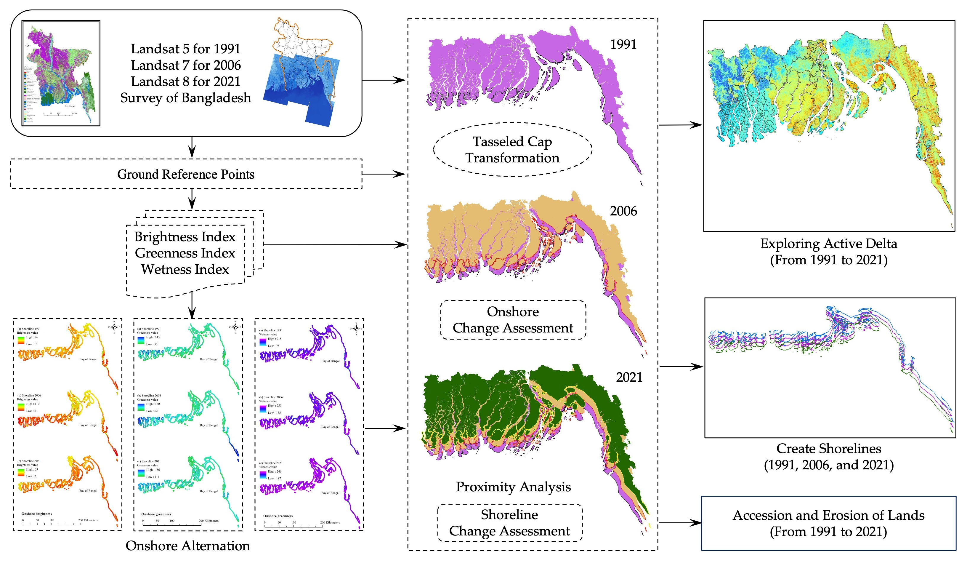
2. Materials and Methods

2.1. Onshore Change Assessment

The onshore change assessment was the first research objective of the study (Figure 1). A comprehensive tasseled cap transformation analysis of onshore alterations was conducted for research on the entire coastal belt of the country using satellite remote sensing datasets.

2.1.1. Geographical Extent of the Study Areas

We considered the coastal belt of Bangladesh consists of a total of 14 administrative districts, including all islands located in the northern Bay of Bengal, allocated inside the maritime boundary of the country (Figure 2). The study area of interest (AoI), with a 710 km long coastline stretching from the Hariabhanga River in the west (along the Bangladesh-India border) to the Naf River in the east (along the Bangladesh-Myanmar border), running parallel to the Bay of Bengal [41], was also considered for the shoreline change assessment (Figure 2). The coastal regions of the country are mainly distributed into three different regions, geo-morphologically named as (i) the South-West Ganges Tidal Plain (western zone), (ii) the South-Central Meghna Deltaic Plain (southern zone), and (iii) the South-East Chittagong Coastal Belt (eastern zone) [41]. Therefore, we illustrated the entire coastal belt as the area of interest (AoI) (Figure 2). The country’s data sheet (CDS), datum WGG84, was checked by the collected geo-database (scale 1:25,000) with the associated topographic feature classes of Bangladesh provided from the Survey of Bangladesh (SoB) under the Ministry of Defense (MoD), Government of Bangladesh (GoB). The eastern zone of Bangladesh is characterized by a muddy shore type in the upper stage of the Chittagong division, while the lower part is dominated by a sandy sea beach area with the world’s longest uninterrupted natural beach [16,21,42,43]. The central zone is geomorphologically the most dynamic part of the active delta due to massive sediment flow from the Ganges-Brahmaputra-Meghna (GBM) river system and strong river currents close to the Meghna estuary [15,44]. Several newly accreted islands, islets, landforms, and shoals are common features of the central estuary zone [13]. Finally, the western zone is principally characterized by the world’s largest mangroves, the Sundarbans Forest [45], including tidal flatlands, swamps, floodplains, and natural levees. Every year, the Sundarbans mangrove forest saves the country as a buffer protection against severe erosion, tropical cyclones, and tidal surges, making the zone relatively stable [24,46].

2.1.2. Collection of Satellite Images

In this study, enhanced thematic mapper Plus (ETM+) and operational land imager (OLI) image dataset (30-m spatial resolution) were collected from Landsat 5, 7 ETM+, and 8 OLI satellites to appropriate spatial resolution and cloud-free coverage for 1991, 2006, and 2021 [47,48]. All Landsat image data were analyzed for the month of November due to hazard and cloud-free datasets separately from the Earth Explorer engine of the United States Geological Survey (USGS). The image acquisition dates for the study years were (i) 19 November 1991 (Landsat 5), (ii) 20 November 2006 (Landsat 7), and (iii) 19 November 2021 (Landsat 8). In this research, bands 1 to 5, band 7 (Landsat 5 and 7 ETM+), and bands 2 to 7 (Landsat 8 OLI) were employed for tasseled cap analysis (Figure 1).

2.1.3. Tasseled Cap Transformation (TCT)

The tasseled cap analysis was introduced by Kauth and Thomas in 1976 and recognized as the Kauth–Thomas transformation [49]. It gives a measure of the three (i) brightness, (ii) greenness, and (iii) wetness indices of the pixel and uses a linear combination of a total of six bands of the Landsat series [27,32]. We utilized the Landsat Toolbox for image processing to make it usable in ArcGIS^® 10.8.2 (ESRI, Redlands, CA 92373, United States) for topographic correction, mosaicking and tasseled cap analysis (Figure 1). Bands 1 to 5 and 7 (visible and infrared): (i) blue ($B_1$ visible), (ii) green ($B_2$ visible), (iii) red ($B_3$ visible), (iv) near infrared ($B_4$ NIR), (v) shortwave infrared ($B_5$ SWIR-1), and (vi) mid-infrared ($B_7$ SWIR-2), respectively. Landsat 5 and 7ETM+ imagery for the tasseled cap analysis was employed to generate three TCT indices of 14 coastal districts. The brightness, greenness, and wetness indices for ETM+ can be computed as the following equations, respectively [49]:

$$B{I}_{ETM+}=\left({\beta }_1·B_1\right)+\left({\beta }_2·B_2\right)+\left({\beta }_3·B_3\right)+\left({\beta }_4·B_4\right)+\left({\beta }_5·B_5\right)+\left({\beta }_7·B_7\right)$$

(1)

$$G{I}_{ETM+}=\left({\epsilon }_1·B_1\right)+\left({\epsilon }_2·B_2\right)+\left({\epsilon }_3·B_3\right)+\left({\epsilon }_4·B_4\right)+\left({\epsilon }_5·B_5\right)+\left({\epsilon }_7·B_7\right)$$

(2)

$$W{I}_{ETM+}=\left({\omega }_1·B_1\right)+\left({\omega }_2·B_2\right)+\left({\omega }_3·B_3\right)+\left({\omega }_4·B_4\right)+\left({\omega }_5·B_5\right)+\left({\omega }_7·B_7\right)$$

(3)

where the computed brightness ($B{I}_{ETM+}$), greenness ($G{I}_{ETM+}$), and wetness ($W{I}_{ETM+}$) indices based on the coefficients ($\beta$), ($\epsilon ),\left(\omega \right),$ and bands ($B$) represent the TOA (top of atmosphere) reflectance, and the coefficients are constants accordingly given below [27].

$$B{I}_{ETM+}=\left(0.3561·B_1\right)+\left(0.3972·B_2\right)+\left(0.3904·B_3\right)+\left(0.6966·B_4\right)+\left(0.2286·B_5\right)+\left(0.1596·B_7\right)$$

$$G{I}_{ETM+}=-\left(0.3344·B_1\right)-\left(0.3544·B_2\right)-\left(0.4556·B_3\right)+\left(0.6966·B_4\right)-\left(0.0242·B_5\right)-\left(0.2630·B_7\right)$$

$$W{I}_{ETM+}=\left(0.2626·B_1\right)+\left(0.2141·B_2\right)+\left(0.0926·B_3\right)+\left(0.0656·B_4\right)-\left(0.7629·B_5\right)-\left(0.5388·B_7\right)$$

Similarly, for the Landsat 8 OLI dataset, bands 2 to 7 (band 1 skipped as coastal/aerosol) were named (i) blue ($B_2$ visible), (ii) green ($B_3$ visible), (iii) red ($B_4$ visible), (iv) near infrared ($B_5$ NIR), (v) shortwave infrared ($B_6$ SWIR-1), and (vi) mid-infrared ($B_7$ SWIR-2), respectively. The brightness, greenness, and wetness indices for OLI can be computed as the following equations, respectively [50]:

$$B{I}_{OLI}=\left({\beta }_2·B_2\right)+\left({\beta }_3·B_3\right)+\left({\beta }_4·B_4\right)+\left({\beta }_5·B_5\right)+\left({\beta }_6·B_6\right)+\left({\beta }_7·B_7\right)$$

(4)

$$G{I}_{OLI}=\left({\epsilon }_2·B_2\right)+\left({\epsilon }_3·B_3\right)+\left({\epsilon }_4·B_4\right)+\left({\epsilon }_5·B_5\right)+\left({\epsilon }_6·B_6\right)+\left({\epsilon }_7·B_7\right)$$

(5)

$$W{I}_{OLI}=\left({\omega }_2·B_2\right)+\left({\omega }_3·B_3\right)+\left({\omega }_4·B_4\right)+\left({\omega }_5·B_5\right)+\left({\omega }_6·B_6\right)+\left({\omega }_7·B_7\right)$$

(6)

where the computed brightness ($B{I}_{OLI}$), greenness ($G{I}_{OLI}$), and wetness ($W{I}_{OLI}$) indices based on the coefficients ($\beta$), ($\epsilon ),\left(\omega \right),$ and bands ($B$) represent the TOA (top of atmosphere) reflectance, and the coefficients were constants accordingly given below [32].

$$B{I}_{OLI}=\left(0.3029·B_2\right)+\left(0.2786·B_3\right)+\left(0.4733·B_4\right)+\left(0.5599·B_5\right)+\left(0.508·B_6\right)+\left(0.1872·B_7\right)$$

$$G{I}_{OLI}=-\left(0.2941·B_2\right)-\left(0.243·B_3\right)-\left(0.5424·B_4\right)+\left(7276·B_5\right)+\left(0.0713·B_6\right)-\left(0.1608·B_7\right)$$

$$W{I}_{OLI}=\left(0.1511·B_2\right)+\left(0.1973·B_3\right)+\left(0.3283·B_4\right)+\left(0.3407·B_5\right)-\left(0.7117·B_6\right)-\left(0.4559·B_7\right)$$

2.1.4. Marking of Shorelines

From the TCT processed in the ArcGIS environment, three new bands, (i) brightness ($B_B$), (ii) greenness ($B_G$), and (iii) wetness ($B_W$), were formed. Among the three new bands, the $B_W$ wetness index was found to be best fitted for the next step named reclassification of lands (Figure 1). Reclassification of the wetness raster $(B_W)$ was obtained from the wetness index raster into two major land cover classes: (i) land and (ii) sea (as waterbodies). The waterbody (river and sea part) class were given a value of 0, and the land class was given a value of 10 by default referring to the Landsat Toolbox. After generating the reclassified land raster for 1991, 2006, and 2021, a reclassified binary image was used to create the shore boundary. The operation of the Landsat Toolbox was designed to create a polyline between the two earlier land use classes. In the process of creating shore boundaries, the area of interest (AoI) was masked to generate precise shore boundaries from the classified land raster set shorelines 1 (1991), 2 (2006), and 3 (2021) (Figure 1).

2.1.5. TCT Analysis of Onshore Alternation

TCT analysis was carried out for onshore alternations by masking (i) brightness ($B_B$), (ii) greenness ($B_G$), and (iii) wetness ($B_W)$ band information using the shorelines of 1991 ($S_1$), 2006 ($S_2$), and 2021 ($S_3$), respectively. Therefore, a total of nine-line rasters of onshore information were prepared for the extensive TCT analysis of onshore changes (Figure 1). The nine obtained line raster(s) of onshore information were considered shoreline brightness ($SB$), shoreline greenness ($SG$), and shoreline wetness ($SW)$ of the study period 1991 ($S{B}_1,S{G}_1,S{W}_1$), 2006 ($S{B}_2,S{G}_2,S{W}_2$), and 2021 ($S{B}_3,S{G}_3,S{W}_3$), respectively.

2.2. Shoreline Change Assessment

We created three shore boundaries for 1991, 2006, and 2021 using a 15-year interval. The shorelines (i) 1991, (ii) 2006, and (iii) 2021 were considered shorelines 1, 2, and 3, respectively, for the next step onshore line change assessment [3]. Therefore, exploring changes among the three shore boundaries, including mainland and island shores, was necessary. In this study, we considered the onshore concept for calculating baselines.

2.2.1. Create Coastal Baseline

A baseline was generated from a novel intersecting layer mask approach of the existing shorelines. We selected three shoreline segments that best represent the study area of interest (Figure 1). For intersecting layer masks, the polygon at the specified shape file and size was selected at the intersection of the three input layers (shoreline 1991, 2006, and 2021). One reference scale was set as the default and set as the reference scale employed for calculating the masking geometry when masks are specified. After calculating the output feature class, the obtained feature class that contained the mask features was used as the baseline of the study. For calculating the coordinate system, we have the spatial reference of the map in which the masking polygons will be created. This is not the spatial reference that will be assigned to the output feature class. It is the spatial reference of the map in which the masking polygons will be used since the position of symbology may change when features are projected.

2.2.2. Ground Reference Points

A total of 16,550 ground reference points were generated by the “vertex to points” application from the study baseline as primary ground reference points (GRPs) for this research. The SoB landmass was used as the dataset and RGB Landsat images (prepared by band combination) of the respective years to confirm the onshore baseline allocated onto land only. Similarly, for the baseline GRPs, we generated GRPs from the shorelines of 1991, 2006, and 2021. For the baseline GRPs, the vertex was found to be 16,550, but for the shorelines, the GRPs were 19,281; 21,945; and 16,548 for 1991, 2006, and 2021, respectively. For equal assessment and GRPs analysis, two vertices were additionally added for the shoreline of 2021, and unnecessary vertices were deleted from the shorelines of 1991 and 2006. During the deleting process, editing tools were used carefully in ArcGIS Desktop. The shoreline-induced and edited 16,550 GRPs of 1991, 2006, and 2021 were also used to extract data from the TCT-generated raster(s).

2.2.3. Accretion and Erosion of Lands (1991 to 2021)

For areal assessment, we applied features to polygon applications from data management tools to generate study baseline polygon features using the AoI. According to a similar process, we prepared AoIs for shoreline 1991, shoreline 2006, and shoreline 2021 polygon features. Thereafter, polygon features were intersected from geoprocessing tools to determine all accretion and erosion of lands into the mainland, islets, and islands of the Bangladesh delta.

2.2.4. Neat Accretion of Lands

Neat accretion was calculated by the difference between accession and erosion of lands from (i) 1991 to 2006, (ii) 1991 to 2021, and (iii) 2006 to 2021 in km². Over the study’s 30-year period, the difference between accession and erosion was considered the actual neat accession of lands of the Bangladesh delta. The actual neat accretion (in km²) was also found to be equal to the difference in the neat accretion of lands from (i) 1991 to 2006 and (ii) 1991 to 2021.

2.2.5. Proximity Analysis

Proximity tools in the ArcGIS environment were distributed into two classes: (i) feature or (ii) raster. In the analysis, the feature type class was used for proximity analysis to calculate the near point distance from the baseline to shorelines (onshore direction) in 1991, 2006, and 2021 using 16,550 GRPs (Figure 1). In the 16,550 GRPs, the point feature file was considered for calculating the point distance. Therefore, the proximity “Near tool” operational feature added the calculated distance measurement attribute to the input features from the onshore direction (Figure 3). Again, the raster-based “Euclidean distance” tools measured distances from the “center of source” cells to the “center of destination” cells. The GRPs on the shoreline were used to calculate near point distance (NPD) in meters and near feature class (NFC) (Figure 3). We calculated NPD 1991, 2006, and 2021 from the study baseline for the years 1991, 2006, and 2021 simultaneously. We reclassified the NPD 1991, 2006, and 2021 GRPs using the natural Jenks classification method into a total of 10 classes for understanding near proximity analysis very clearly to general readers.

2.3. Accuracy Assessment and Comparisons

A total of 16,550 GRPs were used to make the study more precise to identify all types of landforms (Figure 3). Previous studies took part in a small portion, excluding islands, due to the complex setting of the deltaic shorelines. We considered all land areas by utilizing the study GRPs on the SoB country data sheet accurately. The shoreline persuaded and corrected 16,550 GRPs of 1991, 2006, and 2021, which were also utilized to extract point data from the brightness, greenness, and wetness raster(s) named $S{B}_1,S{G}_1,S{W}_1$ of the year 1991, $S{B}_2,S{G}_2,S{W}_2$ raster(s) of the year 2006, and $S{B}_3,S{G}_3,S{W}_3$ raster(s) of the year 2021 accordingly to check the accuracy of the study. All GRPs were also converted to decimal degrees to meters in ArcGIS. Then, we exported the meter GRPs in an Excel spreadsheet and observed that the shoreline shape was also found in the Excel sheet in meters perfectly. In the proximity analysis, all calculations were conducted in linear distance (meter). The analysis also checked Excel^® separately for confirmation using all pixel brightness, greenness, and wetness data.

3. Results

3.1. Onshore Change Assessment

The notion of onshore herein was that the ‘last boundaries’ between ‘land’ and ‘water’ in the Bay of Bengal belong to Bangladesh. The onshore pixel data changed over the decades, including their locational shifts although the deltaic processes of ‘landmass formation’ and ‘coastal bank erosion’ as ‘accretion and erosion of lands’, respectively.

3.1.1. Tasseled Cap Transformation (TCT) of Coastal Districts

The tasseled cap transformation (TCT) method was applied as a remote sensing technique to explore onshore changes in the Bangladesh delta. A total of nine raster(s) datasets with onshore brightness $\left(BI\right)$, greenness $\left(GI\right)$, and wetness $\left(WI\right)$ indices were prepared for the 14 coastal administrative districts of Bangladesh. The BI values in 1991, 2006, and 2021 ranged from 8 to 173 (Figure 4a), 6 to 240 (Figure 4b), and 3 to 129 (Figure 4c), respectively. The GI in 1991, 2006, and 2021 ranged from 33 to 246 (Figure 4d), 5 to 230 (Figure 4e), and 16 to 225 (Figure 4f), respectively. The WI in 1991, 2006, and 2021 ranged from 38 to 234 (Figure 4g), 20 to 249 (Figure 4h), and 3 to 129 (Figure 4i), respectively.

3.1.2. Land Cover Map

Reclassified brightness, greenness, and wetness index raster(s) were experimented to prepare two land cover classes: (i) land and (ii) waterbodies. In this research, the wetness raster(s) gave the best land cover map to prepare land classification. Therefore, the wetness index $\left(WI\right)$ raster transformed into two land cover classes: land and sea (water). The sea part class was found by the value of 0, and the land class type was calculated by the value of 10 according to the default parameter. In the classification process, the land rasters of 1991, 2006, and 2021 were prepared (Figure 5a–c). In the 14 coastal districts, 31,282 (Figure 5a), 31,636 (Figure 5b), and 31,693 (Figure 5c) km² of land were observed in 1991, 2006, and 2021, respectively. The entire longitudinal length, in decimal degrees, was from 89.032 East to 92.358 East. The coast east of Bangladesh, adjacent to the Bay of Bengal, was considered for 1991. It was found from 89.032 East to 92.352 East in 2006 and 89.033 East to 92.346 East in 2021. Every study period, it was moved in east longitudinal coordinates given the changing vibrations of delta shorelines.

3.1.3. Create Shorelines

The shorelines for the respective study years were calculated from the classified land and sea map using the AoI polygon. The classified land area was masked and edited within the AoI area using the cartography toolbox, and the polygon was erased by feature application, except for the shoreline boundaries. The land and sea rasters were reclassified for 1991, 2006, and 2021. The reclassified binary images were transformed into the “create shore boundary” operation of the Landsat Toolbox to create a polyline between the two earlier land use classes. In the process of creating shore boundaries, the area of interest (AoI) was applied to mask the study area (Figure 2) to generate precise shore boundaries as study shorelines 1991 (shape length 3270.59 km), 2006 (shape length 3386.03 km), and 2021 (3338.60 km) (Figure 6). For all shape lengths, the entire coastal belt of the Bangladesh delta was considered, including all large and tiny islands located in the Bay of Bengal inside the SoB, given maritime boundary data sheets (shape files) of the country.

3.1.4. TCT of the Onshore Environment

In the observation of the longitudinal changes (unit decimal degree), wetness values were greater than greenness values, and brightness values were smaller than greenness values. This was repeated for all study years of the research in 1991, 2006, and 2021 (Figure 7a–c). A total of 135,930 pixels were counted in onshore 1991, 111,838 in onshore 1991, and 140,225 in onshore 1991. The mean brightness, greenness, and wetness were 29, 102, and 187, respectively, in 1991 (Figure 7a). In 2006, it was found that the mean brightness, greenness, and wetness changed by 56, 113, and 224, respectively (Figure 7b). The mean values changed to 20 (brightness), 136 (greenness), and 238 (wetness) in 2021 (Figure 7c). In general, onshore greenness and wetness increased from 1991 to 2006 and from 2006 to 2021 consecutively. Only a single decreasing pattern was investigated in the brightness index from 2006 to 2021. Additionally, the brightness index increased from 1991 to 2006.

Onshore Brightness Index

The onshore brightness index was prepared as shore brightness (SB): $S{B}_1$ of 1991 (Figure 8a), $S{B}_2$ of 2006 (Figure 8b), and $S{B}_3$ of 1991 (Figure 8c). The values ranged accordingly from 13 to 86 in 1991 (Figure 8a), 5 to 110 in 2006 (Figure 8b), and 2 to 53 in 2021 (Figure 8c). In the $S{B}_1$ of the year 1991, the 85.78%-pixel data valuation was concentrated from 23 to 36 only from 0 to 255. In 2006, 84.18% of the pixels were agglomerated from 45 to 67 ($S{B}_2$), and 91.11% ranged from 13 to 28 brightness index values in 2021 ($S{B}_3$). Therefore, onshore brightness increased in 2006 from 1991 and decreased in 2021 from 2006 (Figure 9a).

Onshore Greenness Index

The onshore greenness index was made as shore greenness (SG): $S{G}_1$ of the year 1991 (Figure 8d), $S{G}_2$ of the year 2006 (Figure 8e), and $S{G}_3$ of the year 1991 (Figure 8f). The values ranged from 53 to 143 in 1991 (Figure 8d), 62 to 180 in 2006 (Figure 8e), and 111 to 186 in 2021 (Figure 8f). In the $S{G}_1$ of the year 1991, the 88.83%-pixel data valuation was concentrated from 93 to 108 only among 0 to 255. In 2006, 83.16% of the pixels were agglomerated from 101 to 120 ($S{G}_2$), and 88.10% ranged from 123 to 147 greenness index values in 2021 ($S{G}_3$). Therefore, onshore greenness increased frequently from 1991 to 2006 and 2006 to 2021 (Figure 9b).

Onshore Wetness Index

The onshore wetness index was arranged as follows: $S{W}_1$ of the year 1991 (Figure 8g), $S{W}_2$ of the year 2006 (Figure 8h), and $S{W}_3$ of the year 1991 (Figure 8i). The values ranged accordingly from 75 to 215 in 1991 (Figure 8g), 135 to 250 in 2006 (Figure 8h), and 187 to 246 in 2021 (Figure 8i). In the $S{W}_1$ of the year 1991, the 87.73%-pixel data valuation was concentrated from 181 to 196 only among 0 to 255. In 2006, 82.22% of the pixels were agglomerated from 215 to 238 ($S{W}_2$), and 90.58% ranged from 231 to 244 wetness index values in 2021 ($S{W}_3$). Therefore, onshore wetness increased similarly to the greenness index of Bangladesh onshore from 1991 to 2006 and 2006 to 2021 (Figure 9c).

3.1.5. Onshore TCT Change Comparisons

TCT analysis provides linear relationships among (i) brightness, (ii) greenness, and (iii) wetness combinations. This study exemplified the linear combination of three band features: TCT-BG (brightness and greenness) (Figure 10a–c), TCT-BW (brightness and wetness) (Figure 10d–f), and TCT-WG (greenness and wetness) (Figure 10g–i). From the TCT at-satellite reflectance of the three main uncorrelated indices, it was observed that the brightness index as a measurement value for the onshore ground surface was reduced. Therefore, greenness increased gradually in parallel with the wetness index. The greenness index, as a measurement value for the phenology of vegetation, significantly provided information positively that the Bangladesh delta will also be greener in the future. The yellow stuff belongs to the wetness index, which is the representation of soil and vegetation, as the information of plant canopy moisture interacted gradually to improve greenness, usually to attain a degree of acceptance of this TCT application onshore remote sensing.

3.2. Shoreline Change Assessment

In the onshore change assessment, pixel TCT properties changed over the periods of 1991, 2006, and 2021 (Figure 10a–i). The shorelines were shifted geographically, and the second portion of this study was focused on the shoreline change assessment of the Bangladesh delta in 2006 from 1991 and 2021 from 1991 and 2006, and from the study baseline of the Bangladesh coast.

3.2.1. Baseline Assessment and GRPs

Three shorelines for 1991, 2006, and 2021 for a period of 15 years intervals were utilized for the change assessment (Figure 6 and Figure 11a). The shorelines of 1991, 2006, and 2021 were explored using onshore changes among the three shore boundaries, including mainland and island shores (Figure 11a). In intersecting layer mask processing, the study baseline was created (Figure 11a). In the study, the baseline was taken onshore (Figure 11b). For areal analysis, the upper line of the AoI was combined with the acquired, baseline, shoreline 1991, 2006, and 2021 (Figure 11a). In this research, the point, line, and polygon shape features were embedded with the AoI (Figure 2) to assess shoreline changes. The baseline length was calculated to be 2633.12 km (Figure 11b). Point features were based on a total of 16,550 GRPs (Figure 11c), line features were from the created shore boundaries (Figure 11a), and thirdly, polygonal features were generated from the area assessment stage (Figure 12a–d) as part of the AoI area assessment, land accretion from the baseline, land accretion, and erosion in the respective study years in the Bay of Bengal of the Bangladesh territory.

3.2.2. Area Assessment of Study Lands Using the AoI Mask

In the study, the baseline induced base-land AoI was 7572.81 km² (Figure 12a). The AoI-based study-lands were assessed in 1991 (8448.81 km²), 2006 (8798.09 km²), and 2021 (8872.03 km²) accordingly (Figure 12b–d). Therefore, the polygonal shapes represented that the shoreline adjacent areas were changed, and the overall lands were accredited for the area increasing pattern of the coastal areas in Bangladesh.

3.2.3. Accretion of Lands (Baseline to Shorelines)

The total land accretion with a baseline for 1991, 2006, and 2021 was observed through the distribution among the coastal areas (Figure 13a–c). Additionally, land accretion was listed as 876.01 km², 1225.28 km², and 1299.22 km² in 1991, 2006, and 2021, respectively (

Table 1. Accession of lands from baseline to shoreline.

From Baseline	Accretion (km2)
To shoreline of 1991	876.01
To shoreline of 2006	1225.28
To shoreline of 2021	1299.22

). The study baseline was obtained as intersected layer masks among all shorelines, and therefore, no erosion of the baseline was found (Figure 11a).

3.2.4. Neat Accretion and Erosion of Lands (Shoreline to Shoreline)

The baseline was constantly used for the study to obtain accessions and erosion from the shoreline to the shoreline accordingly (

Table 2. Changes in accession and erosion of lands along shorelines.

Shoreline	Accretion (km2)	Erosion (km2)	Neat Accretion (km2)
1991 to 2006	825.15	475.87	349.28
1991 to 2021	1223.94	800.72	423.22
2006 to 2021	756.69	682.75	73.94 *

* Actual neat eat accretion over 30 years from 1991 to 2021.

). In Figure 14a, a total of 825.15 km² of land was accredited in 2006 from the 1991 shoreline with 475.87 km² of coastal erosion (Table 2). Figure 14b shows that a total of 1223.94 km² of land was accredited in 2021 from the 1991 shoreline with 800.72 km² of coastal erosion (Table 2). Therefore, the study revealed that from 1991 to 2021, the neat accession was 73.94 km² (Table 2). By Figure 14c, the land accession and erosion were observed to be 756.69 km² and 682.75 km², respectively, from 2006 to 2021 (Table 2).

3.2.5. Proximity Analysis: Near Point Distance and Near Feature

Proximity analysis was employed to calculate the relationship between the selected 16,550 ground reference points and their neighbors (Figure 11c and Figure 15a–c). We also calculated the entire shape length of the study baseline and shorelines (Figure 11b). Additionally, near point distance (NPD) classes of 1991 (natural Jenks in meters) from baseline points to shoreline points were also calculated to understand shoreline change classification in the Bay of Bengal area of Bengal delta (Figure 15a for the study year 1991, Figure 15b for the study year 2006, Figure 15c for the study year 2021). It was also classified to prepare NPD classes (

Table 3. Count (number) and percentage of baseline GRPs by near point distance (NPD) classes to shorelines.

		NPD-1 (1991)		NPD-2 (2006)		NPD-3 (2021)
Class Number	NPD Class (m)	Count	%	Count	%	Count	%
1	0–136.65	8301	50.16	7886	47.65	8568	51.77
2	136.66–379.51	2827	17.08	3611	21.82	1249	7.55
3	379.52–746.59	1547	9.35	1363	8.24	1214	7.34
4	746.60–1334.52	1128	6.82	1034	6.25	1204	7.27
5	1334.53–2086.62	790	4.77	847	5.12	938	5.67
6	2086.63–3050.70	840	5.08	566	3.42	772	4.66
7	3050.71–4432.38	529	3.20	587	3.55	1009	6.10
8	4432.39–6738.46	298	1.80	247	1.49	1032	6.24
9	6738.47–9540.68	242	1.46	115	0.69	364	2.20
10	9540.69–17,159.42	48	0.29	294	1.78	200	1.21
	Total	16,550	100	16,550	100	16,550	100

), which gives us a clear view of the Bangladesh shoreline movement within the last three decades from 1991 to 2021 (Figure 15a–c). Finally, the shoreline points as near-distance features for 1991 (Figure 15a), 2006 (Figure 15b), and 2021 (Figure 15c) were used for assessing near-feature GRPs by baseline points (

Table 4. Near feature analysis of the study baseline ground reference points (GRPs) for validation.

Near Shoreline Feature	Baseline GRPs		Avg. Distance from Baseline (in m)
	Count	%
Shoreline of 1991	5935	35.86	245.45
Shoreline of 2006	3305	19.97	474.84
Shoreline of 2021	7310	44.17	379.19
Total	16,550	100

). Near features of the study were observed by point-to-point proximity analysis using location (optional) tick marks in the near proximity assessment (Table 4).

3.3. Accuracy Assessment

This study was conducted utilizing 16,550 vertices to points of the baseline as GRPS (Figure 11a–c). These GRPs were settled into the landmass of the country that was verified by the SoB country datasheet, and these landmasses have never faced any land erosion activities since 1991 to date. Therefore, we projected the degree decimal points features to meter points features graphically using Microsoft Excel^®. Similar results were obtained from the Excel analysis for the research and were good-fitted evidence. We obtained comparisons among NPD 1991, 2006, and 2021 classes, and listed them in Table 3. The changes in Bangladesh shorelines in the range from 1991 to 2021 were observed with a 15-year interval in 2006 (Table 4).

4. Discussion

The shoreline of coastal areas has changed frequently over the decades. Although it is a natural process, it has a vital role in influencing coastal livelihoods in the country due to densely populated coastal regions. In 1991, the Landsat 5 dataset was excellent compared with the 2006 Landsat 7 dataset. The limitations of the study were the ‘Landsat Toolbox’ provided ‘Repair Landsat 7 ETM+ Band’ had been used for necessary corrections of 2006’s Landsat 7 datasets. The Landsat 8 OLI bands were excellent. All the calculations were performed in meters (m) for point and line distances and in square kilometers (km²) for polygonal area assessment. Bangladesh has a 710 km-long coastline stretching from the Hariabhanga River in the west (along the Bangladesh–India border) to the Naf River in the east (along the Bangladesh–Myanmar border), running parallel to the Bay of Bengal (Matin and Hasan 2021). However, after considering all islands, isles, islets, and riverine shoreline shapes, including mainland shore boundaries, we found land and water (sea) demarcation shapes (in km) of 3270 km in the shoreline year 1991, 3386 km in 2006, and 3338 km in 2021 (Figure 11a). This length calculation was only inside the AoI coastal belt of the entire Bangladesh delta (Figure 12). The calculated baseline shape length (2633.12 km) was less than all shorelines for the intersecting loss of many small islands (Figure 11b). In the study, the baseline-induced base-land AoI was 7572.81 km² (Figure 12a). In addition, we found it to increase among all AoI-based study land in 1991 (8448.81 km²), 2006 (8798.09 km²), and 2021 (8872.03 km²) (Figure 12b,c). Therefore, a clear view of the country observed that the shorelines are moving toward change, and overall lands were accredited for the area increasing aspects of the Bangladesh delta.

Matin and Hasan (2021) investigated the net area loss and gain of the Bangladesh delta by three zonal classes: west zone 40.67 km² (neat erosion), central zone 61.69 km² loss (neat erosion), and eastern zone 30.20 km² (neat accession) from 1989 to 2019. Sarwar and Woodroffe (2013) found that the total area along the Bangladesh shoreline changed slightly across the whole shoreline from 1989 to 2009 (20 years), with 315 km² of accretion and approximately 307 km² of erosion. In this study, in detail, neat accretion and erosion were calculated. From 1991 to 2006, the total accredited land area was 825.15 km² (Figure 14a). However, it was 756.69 km² from 2006 to 2021 (Figure 14c) (Table 2). Thus, we obtained total accretion from 1991 to 2021 over the 30-year period of 1223.94 km² (Figure 14b) (Table 2). In the case of coastal erosion assessment, the results gained for the period 1991 to 2006 and 2006 to 2021 were 475.87 km² (Figure 14a) and 682.75 (Figure 14c) km², respectively (Table 2). Therefore, the total coastal erosion was 800.72 km² from 1991 to 2021 (Figure 14c) (Table 2). Therefore, the net accretion was 73.94 km² from 1991 to 2021 (Table 2). This can be proof that the Bangladesh delta is active and increasing towards frequent change. If the erosion process is increasing, it can be threatened for coastal people to continue their livelihoods in relation to climate change and sea level rise issues. In the study, erosion also considered landmass sinking and accretion related to land level rise due to sediment load deposition on the continental shelf of the Bay of Bengal. Table 4 represents the near feature of the study baseline GRPs from the calculated three shoreline features as another result of shoreline changes in the Bay of Bengal. Further research is also significantly required to understand the impacts of shoreline alternations on land use and livelihoods changes. In this stage of this research, we could predict the alternations process from 30 years of datasets. In our next stages, the impact of shoreline alternations will be carried out considering extreme climatic events.

5. Conclusions

Bangladesh is a country with a dense population and diversified riverine and deltaic landforms. A detailed shoreline assessment and change assessment study is required to support the delta plan implementation activities of the country government. Bangladesh coastal areas are increasing, but the rates were slower after the period 1991–2006 in 2006–2021. In the 15-year period from 2006 to 2021, the erosion rate also increased. New lands could be added with the country datasheet that was collected from the Survey of Bangladesh office of the government. This study was important to prepare accurate mapping of the southern parts. There was a large gap found in the government offices—that they do not have updated or finalized shoreline boundaries (shape files) that are necessary for the respective year. In this study, we prepared shoreline boundaries for 1991, 2006, and 2021 as the country’s shoreline boundary in the Bay of Bengal. This research can be utilized for future studies, and similarly, other researchers can build up shore boundaries, including changes over time, for future projections of land use planning.

References

1. Boak, E.H.; Turner, I.L. Shoreline Definition and Detection: A Review. J. Coast. Res. 2005, 214, 688–703. [Google Scholar] [CrossRef] [Green Version]
2. Matin, N.; Hasan, G.M.J. A quantitative analysis of shoreline changes along the coast of Bangladesh using remote sensing and GIS techniques. CATENA 2021, 201, 105185. [Google Scholar] [CrossRef]
3. Leatherman, S.P. Chapter 8 Social and Economic Costs of Sea Level Rise. In International Geophysics; Academic Press: Cambridge, MA, USA, 2001; Volume 75, pp. 181–223. [Google Scholar] [CrossRef]
4. Rahman, A.F.; Dragoni, D.; El-Masri, B. Response of the Sundarbans coastline to sea level rise and decreased sediment flow: A remote sensing assessment. Remote Sens. Environ. 2011, 115, 3121–3128. [Google Scholar] [CrossRef]
5. Ford, M. Shoreline changes interpreted from multi-temporal aerial photographs and high-resolution satellite images: Wotje Atoll, Marshall Islands. Remote Sens. Environ. 2013, 135, 130–140. [Google Scholar] [CrossRef]
6. Pardo-Pascual, J.E.; Almonacid-Caballer, J.; Ruiz, L.A.; Palomar-Vázquez, J. Automatic extraction of shorelines from Landsat TM and ETM+ multi-temporal images with subpixel precision. Remote Sens. Environ. 2012, 123, 1–11. [Google Scholar] [CrossRef] [Green Version]
7. Al-Maruf, A.; Jenkins, J.C.; Bernzen, A.; Braun, B. Measuring household resilience to cyclone disasters in coastal Bangladesh. Climate 2021, 9, 97. [Google Scholar] [CrossRef]
8. Wang, X.-Z.; Zhang, H.-G.; Fu, B.; Shi, A. Analysis on the coastline change and erosion-accretion evolution of the Pearl River Estuary, China, based on remote-sensing images and nautical charts. J. Appl. Remote Sens. 2013, 7, 073519. [Google Scholar] [CrossRef] [Green Version]
9. Dube, S.K.; Chittibabu, P.; Sinha, P.C.; Rao, A.D.; Murty, T.S. Numerical Modelling of Storm Surge in the Head Bay of Bengal Using Location Specific Model. Nat. Hazards 2004, 31, 437–453. [Google Scholar] [CrossRef]
10. Shamsuzzoha, M.; Noguchi, R.; Ahamed, T. Rice yield loss area assessment from Satellite-derived NDVI after extreme climatic events using a fuzzy approach. Agric. Inf. Res. 2021, 31, 32–46. [Google Scholar] [CrossRef]
11. Bala, B.K.; Hossain, M.A. Modeling of food security and ecological footprint of coastal zone of Bangladesh. Environ. Dev. Sustain. 2010, 12, 511–529. [Google Scholar] [CrossRef]
12. Hussain, M.A.; Tajima, Y.; Gunasekara, K.; Rana, S.; Hasan, R. Recent coastline changes at the eastern part of the Meghna Estuary using PALSAR and Landsat images. IOP Conf. Ser. Earth Environ. Sci. 2014, 20, 012047. [Google Scholar] [CrossRef] [Green Version]
13. McGranahan, G.; Balk, D.; Anderson, B. The rising tide: Assessing the risks of climate change and human settlements in low elevation coastal zones. Environ. Urban. 2007, 19, 17–37. [Google Scholar] [CrossRef]
14. Rahaman, M.A.; Mursheduzzaman Ali Reza GA, M.; Chowdhury, A.M.; Avi, A.R.; Chakraborty, T.R.; Shamsuzzoha, M. Nature-Based Solutions to Promote Climate Change Adaptation and Disaster Risk Reduction Along the Coastal Belt of Bangladesh. In The Palgrave Handbook of Climate Resilient Societies; Palgrave Macmillan: Cham, Switzerland, 2020. [Google Scholar] [CrossRef]
15. Kabir, M.A.; Salauddin, M.; Hossain, K.T.; Tanim, I.A.; Saddam MM, H.; Ahmad, A.U. Assessing the shoreline dynamics of Hatiya Island of Meghna estuary in Bangladesh using multiband satellite imageries and hydro-meteorological data. Reg. Stud. Mar. Sci. 2020, 35, 101167. [Google Scholar] [CrossRef]
16. Mahamud, U.; Takewaka, S. Shoreline Change around a River Delta on the Cox’s Bazar Coast of Bangladesh. J. Mar. Sci. Eng. 2018, 6, 80. [Google Scholar] [CrossRef] [Green Version]
17. Talukder, M.F.; Shamsuzzoha, M.; Hasan, I. Damage and Agricultural Rehabilitation Scenario of Post Cyclone Mahasen in Coastal Zone of Bangladesh. J. Sociol. Anthropol. 2018, 2, 36–43. [Google Scholar]
18. Shamsuzzoha, M.; Al-Maruf, A. Post SIDR life strategy: Adaptation scenario of settlements of the south. Inst. Bangladesh Stud. (IBS) J. 2012, 19, 207–222. [Google Scholar]
19. Ataol, M.; Kale, M.M. Shoreline changes in the river mouths of the Ceyhan Delta. Arab. J. Geosci. 2022, 15, 201. [Google Scholar] [CrossRef]
20. Crawford, T.W.; Rahman, M.K.; Miah, M.G.; Islam, M.R.; Paul, B.K.; Curtis, S.; Islam, M.S. Coupled Adaptive Cycles of Shoreline Change and Households in Deltaic Bangladesh: Analysis of a 30-Year Shoreline Change Record and Recent Population Impacts. Ann. Am. Assoc. Geogr. 2021, 111, 1002–1024. [Google Scholar] [CrossRef]
21. Islam, M.A.; Hossain, M.S.; Hasan, T.; Murshed, S. Shoreline changes along the Kutubdia Island, southeast Bangladesh using digital shoreline analysis system. Bangladesh J. Sci. Res. 2016, 27, 99–108. [Google Scholar] [CrossRef] [Green Version]
22. Mahamud, U.; Takewaka, S. Temporal and spatial characteristics of shoreline variability at Cox’s Bazar, Bangladesh. J. Jpn. Soc. Civ. Eng. Ser. B2 2016, 72, I_715–I_720. [Google Scholar] [CrossRef] [PubMed]
23. Natarajan, L.; Sivagnanam, N.; Usha, T.; Chokkalingam, L.; Sundar, S.; Gowrappan, M.; Roy, P.D. Shoreline changes over last five decades and predictions for 2030 and 2040: A case study from Cuddalore, southeast coast of India. Earth Sci. Inform. 2021, 14, 1315–1325. [Google Scholar] [CrossRef]
24. Sarwar Md, G.M.; Woodroffe, C.D. Rates of shoreline change along the coast of Bangladesh. J. Coast. Conserv. 2013, 17, 515–526. [Google Scholar] [CrossRef] [Green Version]
25. Costantino, D.; Pepe, M.; Dardanelli, G.; Baiocchi, V. Using optical satellite and aerial imagery for automatic coastline mapping. Geogr. Tech. 2020, 15, 171–190. [Google Scholar] [CrossRef]
26. Dominici, D.; Zollini, S.; Alicandro, M.; Della Torre, F.; Buscema, P.M.; Baiocchi, V. High Resolution Satellite Images for Instantaneous Shoreline Extraction Using New Enhancement Algorithms. Geosciences 2019, 9, 123. [Google Scholar] [CrossRef] [Green Version]
27. Huang, C.; Wylie, B.; Yang, L.; Homer, C.; Zylstra, G. Derivation of a tasselled cap transformation based on Landsat 7 at-satellite reflectance. Int. J. Remote Sens. 2002, 23, 1741–1748. [Google Scholar] [CrossRef]
28. Sheng, L.; Huang, J.; Tang, X. A tasseled cap transformation for CBERS-02B CCD data. J. Zhejiang Univ. SCIENCE B 2011, 12, 780–786. [Google Scholar] [CrossRef] [Green Version]
29. Crist, E.P. A TM Tasseled Cap equivalent transformation for reflectance factor data. Remote Sens. Environ. 1985, 17, 301–306. [Google Scholar] [CrossRef]
30. Crist, E.P.; Cicone, R.C. Comparisons of the dimensionality and features of simulated Landsat-4 MSS and TM data. Remote Sens. Environ. 1984, 14, 235–246. [Google Scholar] [CrossRef]
31. Zhai, Y.; Roy, D.P.; Martins, V.S.; Zhang, H.K.; Yan, L.; Li, Z. Conterminous United States Landsat-8 top of atmosphere and surface reflectance tasseled cap transformation coefficients. Remote Sens. Environ. 2022, 274, 112992. [Google Scholar] [CrossRef]
32. Baig, M.H.A.; Zhang, L.; Shuai, T.; Tong, Q. Derivation of a tasselled cap transformation based on Landsat 8 at-satellite reflectance. Remote Sens. Lett. 2014, 5, 423–431. [Google Scholar] [CrossRef]
33. Dymond, C.C.; Mladenoff, D.J.; Radeloff, V.C. Phenological differences in Tasseled Cap indices improve deciduous forest classification. Remote Sens. Environ. 2002, 80, 460–472. [Google Scholar] [CrossRef]
34. Healey, S.; Cohen, W.; Zhiqiang, Y.; Krankina, O. Comparison of Tasseled Cap-based Landsat data structures for use in forest disturbance detection. Remote Sens. Environ. 2005, 97, 301–310. [Google Scholar] [CrossRef]
35. Mbow, C.; Goïta, K.; Bénié, G.B. Spectral indices and fire behavior simulation for fire risk assessment in savanna ecosystems. Remote Sens. Environ. 2004, 91, 1–13. [Google Scholar] [CrossRef]
36. Serra, P.; Pons, X. Monitoring farmers’ decisions on Mediterranean irrigated crops using satellite image time series. Int. J. Remote Sens. 2008, 29, 2293–2316. [Google Scholar] [CrossRef]
37. Wulder, M.A.; Skakun, R.S.; Kurz, W.A.; White, J.C. Estimating time since forest harvest using segmented Landsat ETM+ imagery. Remote Sens. Environ. 2004, 93, 179–187. [Google Scholar] [CrossRef]
38. Anwar, M.S.; Takewaka, S. Analyses on phenological and morphological variations of mangrove forests along the southwest coast of Bangladesh. J. Coast. Conserv. 2014, 18, 339–357. [Google Scholar] [CrossRef]
39. Emran, A.; Rob, M.A.; Kabir, M.H. Coastline Change and Erosion-Accretion Evolution of the Sandwip Island, Bangladesh. Int. J. Appl. Geospat. Res. 2017, 8, 33–44. [Google Scholar] [CrossRef]
40. Alam, S.; de Heer, J.; Choudhury, G. Bangladesh Delta Plan 2100. 2018. Available online: http://www.plancomm.gov.bd/site/files/0adcee77-2db8-41bf-b36b-657b5ee1efb9/Bangladesh-Delta-Plan-2100 (accessed on 9 September 2022).
41. Karim, M.; Mimura, N. Impacts of climate change and sea-level rise on cyclonic storm surge floods in Bangladesh. Glob. Environ. Chang. 2008, 18, 490–500. [Google Scholar] [CrossRef]
42. BBC. World’s Longest Natural Sea Beach under Threat. 26 December 2012. Available online: https://www.bbc.com/news/av/world-asia-20699989 (accessed on 28 September 2022).
43. Hasan, M.M.; Islam, R.; Rahman, M.S. Analysis of Land Use and Land Cover Changing Patterns of Bangladesh Using Remote Sensing Technology. Am. J. Environ. Sci. 2021, 17, 64–74. [Google Scholar] [CrossRef]
44. Alam, R. Characteristics of Hydrodynamic Processes in the Meghna Estuary due to Dynamic Whirl Action. IOSR J. Eng. 2014, 4, 39–50. [Google Scholar] [CrossRef]
45. Akbar Hossain, K.; Masiero, M.; Pirotti, F. Land cover change across 45 years in the world’s largest mangrove forest (Sundarbans): The contribution of remote sensing in forest monitoring. Eur. J. Remote Sens. 2022, 1–17. [Google Scholar] [CrossRef]
46. Rogers, K.G.; Goodbred, S.L. The Sundarbans and Bengal Delta: The World’s Largest Tidal Mangrove and Delta System; Springer: Dordrecht, The Netherlands, 2014; pp. 181–187. [Google Scholar] [CrossRef]
47. Che, X.; Zhang, H.K.; Liu, J. Making Landsat 5, 7 and 8 reflectance consistent using MODIS nadir-BRDF adjusted reflectance as reference. Remote Sens. Environ. 2021, 262, 112517. [Google Scholar] [CrossRef]
48. Shamsuzzoha, M.; Noguchi, R.; Ahamed, T. Damaged area assessment of cultivated agricultural lands affected by cyclone bulbul in coastal region of Bangladesh using Landsat 8 OLI and TIRS datasets. Remote Sens. Appl. Soc. Environ. 2021, 23, 100523. [Google Scholar] [CrossRef]
49. Mondal, A.; Khare, D.; Kundu, S.; Mondal, S.; Mukherjee, S.; Mukhopadhyay, A. Spatial soil organic carbon (SOC) prediction by regression kriging using remote sensing data. Egypt. J. Remote Sens. Space Sci. 2017, 20, 61–70. [Google Scholar] [CrossRef] [Green Version]
50. Dzakiyah, I.F.; Saraswati, R. Drought area of agricultural land using Tasseled Cap Transformation (TCT) method in Ciampel Subdistrict Karawang Regency. E3S Web Conf. 2020, 211, 02005. [Google Scholar] [CrossRef]
Figure 1. Research framework for determining onshore change and shoreline change assessments.
Remotesensing 15 00295 g001
Figure 2. The study area (Datum WGG84): total 14 coastal districts and area of interest (AoI).
Remotesensing 15 00295 g002
Figure 3. Proximity analysis of the study.
Remotesensing 15 00295 g003
Figure 4. Brightness index: (a) 1991, (b) 2006, and (c) 2021; Greenness index: (d) 1991, (e) 2006, and (f) 2021; Wetness index: (g) 1991, (h) 2006, and (i) 2021 of coastal districts, Bangladesh delta.
Remotesensing 15 00295 g004
Figure 5. Reclassification of lands of coastal districts: (a) 1991, (b) 2006, and (c) 2021.
Remotesensing 15 00295 g005aRemotesensing 15 00295 g005b
Figure 6. Study shoreline combinations of Bangladesh from 1991 to 2021 (15-year interval).
Remotesensing 15 00295 g006
Figure 7. Onshore TCT and longitudinal changes (decimal degree): (a) 1991, (b) 2006, and (c) 2021.
Remotesensing 15 00295 g007
Figure 8. Onshore brightness index: (a) S B 1 of 1991, (b) S B 2 of 2006, and (c) S B 3 of 2021; Onshore greenness index: (d) S G 1 of 1991, (e) S G 2 of 2006, and (f) S G 3 of 2021; Onshore wetness index: (g) S W 1 of 1991, (h) S W 2 of 2006, and (i) S W 3 of 2021 of coastal districts, Bangladesh delta.
Remotesensing 15 00295 g008
Figure 9. Onshore TCT change statistics: (a) brightness, (b) greenness, and (c) wetness.
Remotesensing 15 00295 g009
Figure 10. Onshore TCT change comparisons: (a) TCT-BG of 1991, (b) TCT-BG of 2006, and (c) TCT-BG of 2021, (d) TCT-BW of 1991, (e) TCT-BW of 2006, and (f) TCT-BW of 2021, (g) TCT-WG of 1991, (h) TCT-WG of 2006, and (i) TCT-WG of 2021.
Remotesensing 15 00295 g010
Figure 11. Baseline assessment and validation by ground reference points (GRPs) using the SoB-provided country datasheet of Bangladesh: (a) create coastal baseline, (b) point and line features intersection of baseline, and (c) total 16,550 baseline GRPs.
Remotesensing 15 00295 g011aRemotesensing 15 00295 g011b
Figure 12. Area assessment using AoI Mask: (a) base land, (b) study land (1991), (c) study land (2006), and (d) study land (2021).
Remotesensing 15 00295 g012
Figure 13. Land accretion along with the study baseline in the coastal region of Bangladesh (baseline to shoreline): (a) 1991, (b) 2006, and (c) 2021.
Remotesensing 15 00295 g013aRemotesensing 15 00295 g013b
Figure 14. Cumulative accretion and erosion of lands in the coastal region of Bangladesh (shoreline to shoreline): (a) 1991 to 2006, (b) 1991 to 2021, and (c) 2006 to 2021.
Remotesensing 15 00295 g014aRemotesensing 15 00295 g014b
Figure 15. Near point distance (NPD) in meters using proximity analysis (baseline to the shoreline): (a) NPD-1 of 1991, (b) NPD-2 of 2006, and (c) NPD-3 of 2021.
Remotesensing 15 00295 g015aRemotesensing 15 00295 g015b