
New Approach for Photogrammetric Rock Slope Premonitory Movements Monitoring


Abstract
:1. Introduction
2. Methodology
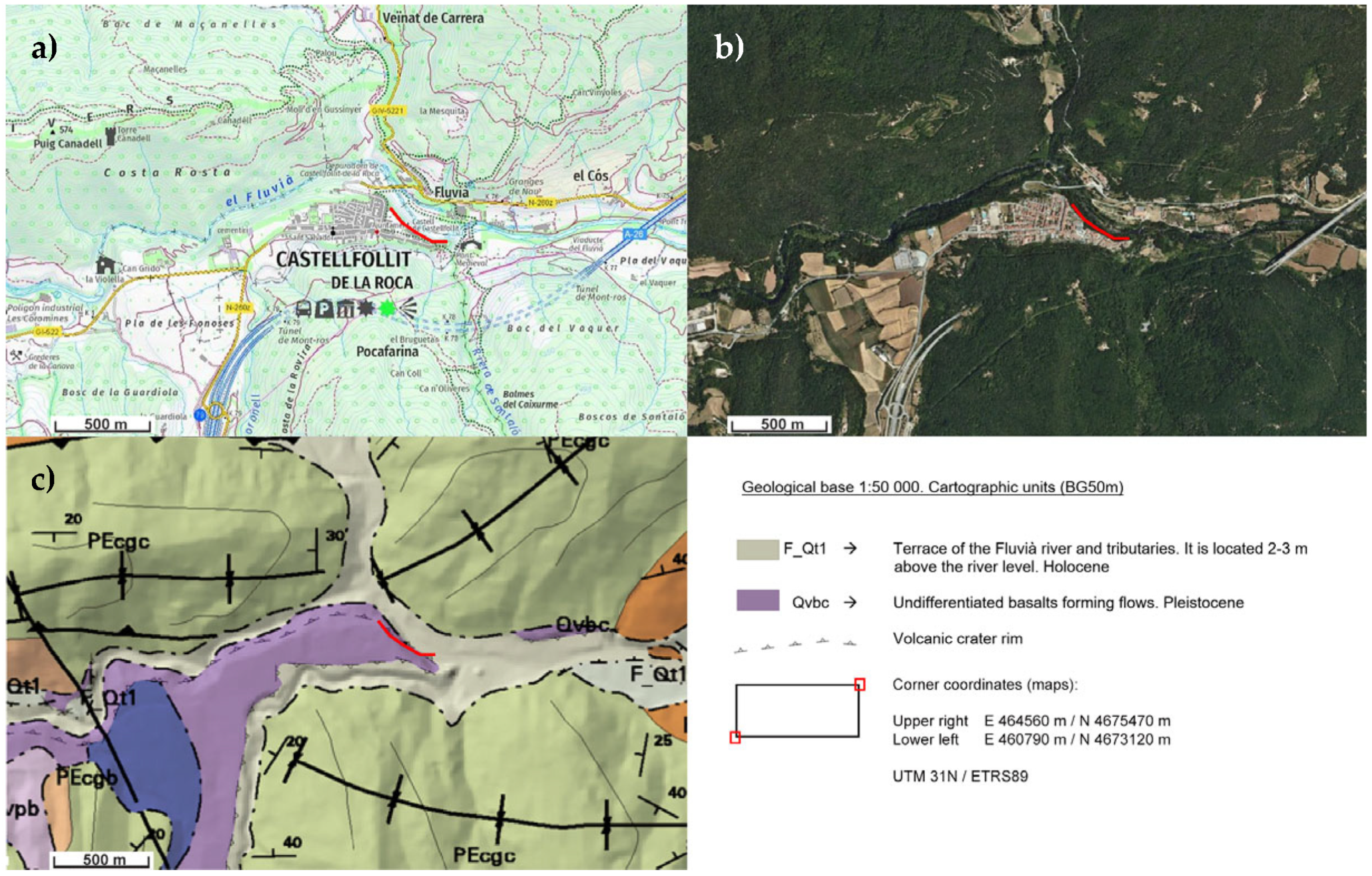
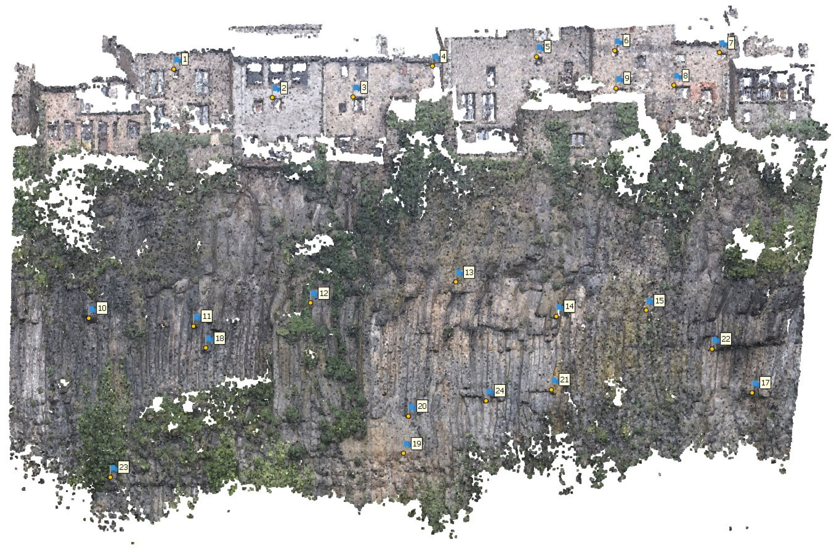
2.1. Study Site
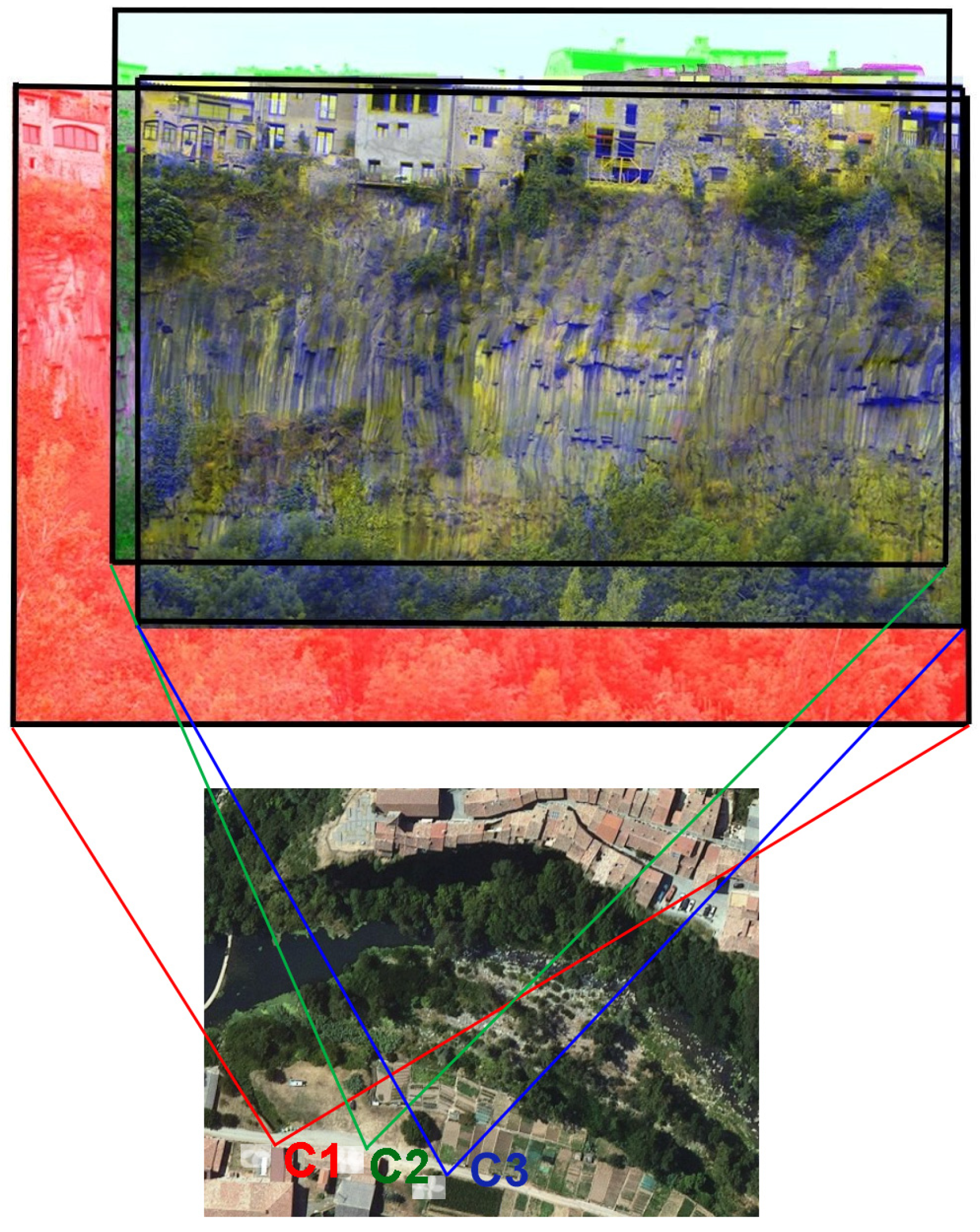
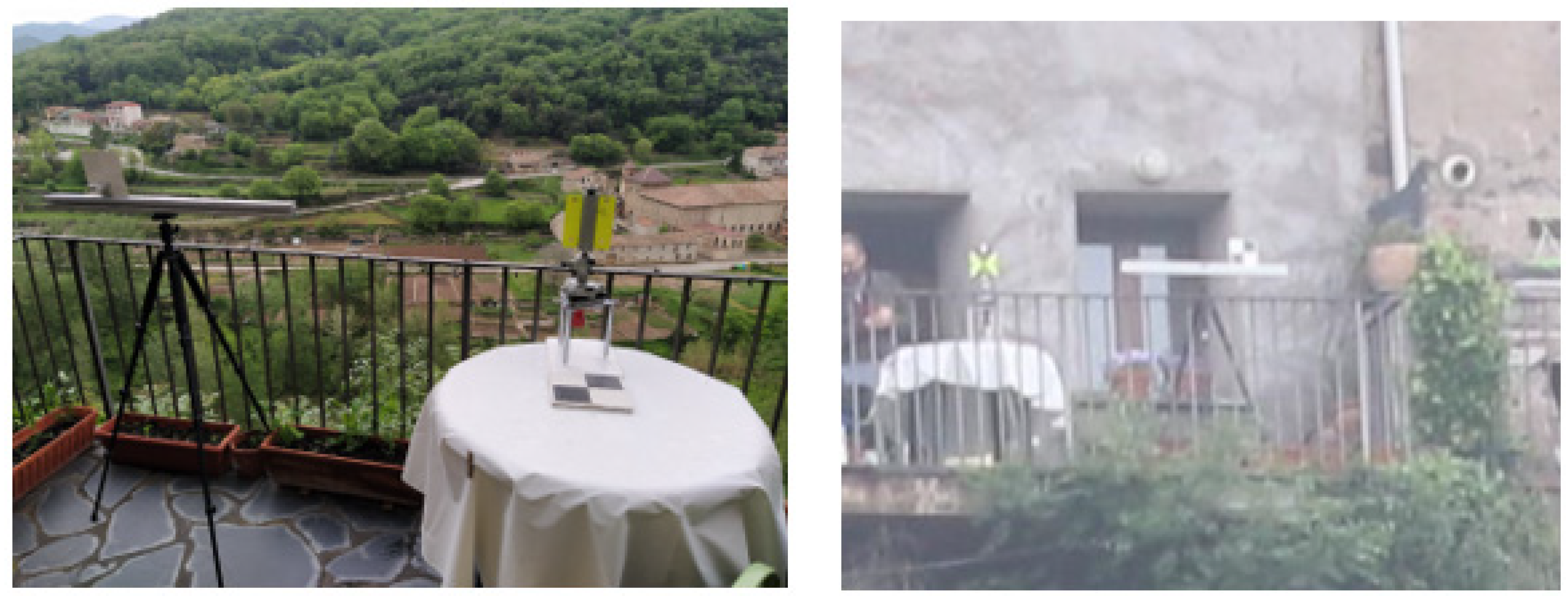
2.2. System Design
2.3. Error Analysis in 3D Photogrammetric Models
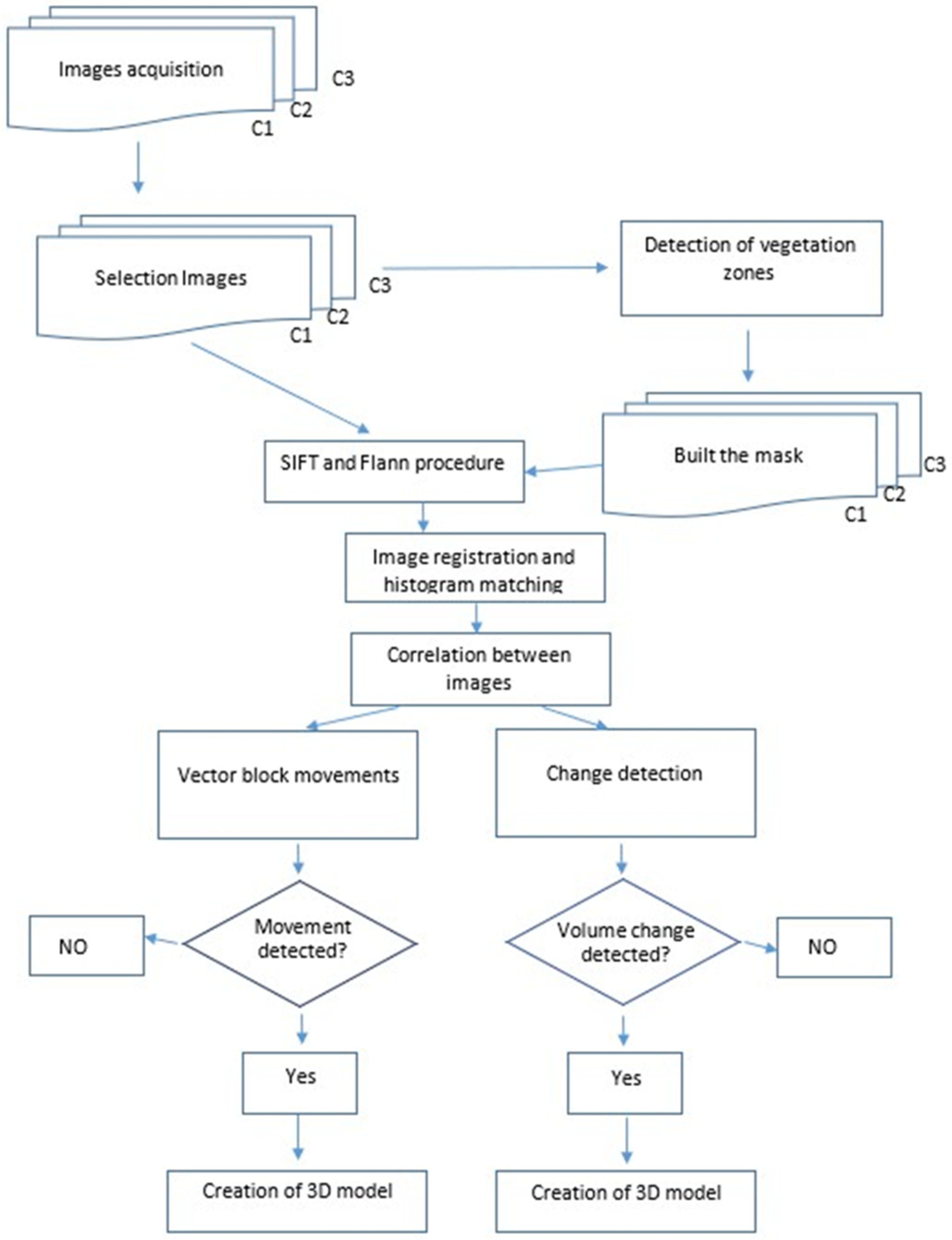
2.4. Processing Approach
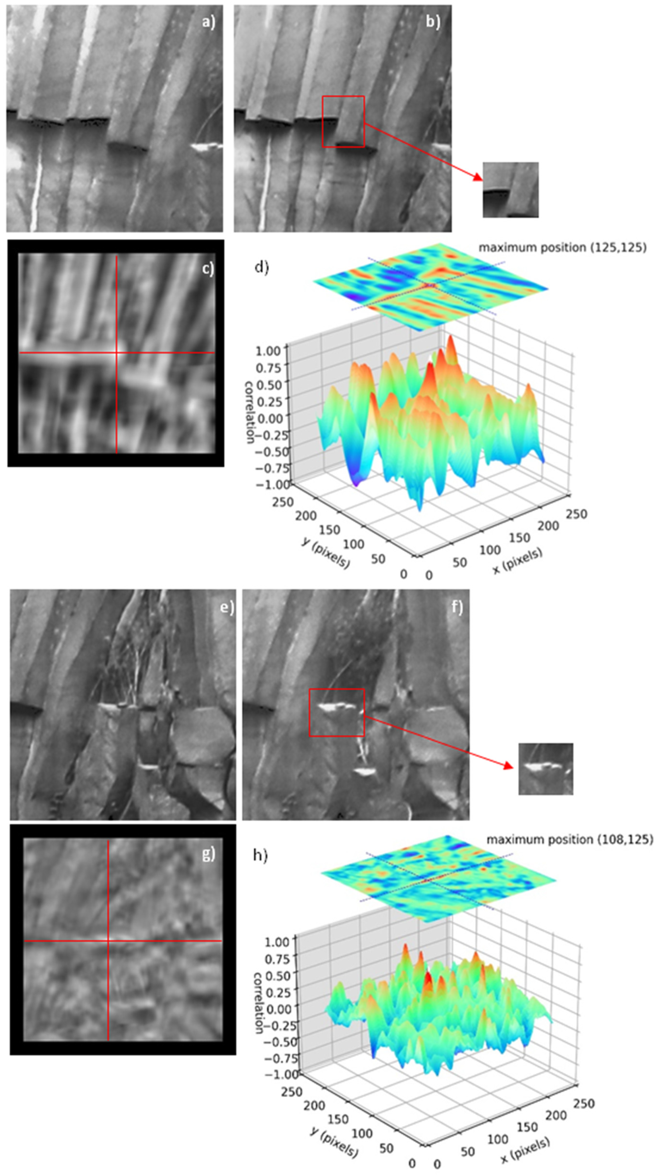
2.5. Image Processing
- A.
- Image Adjustment
- B.
- Movement detection
- C.
- Model building. Movement quantification
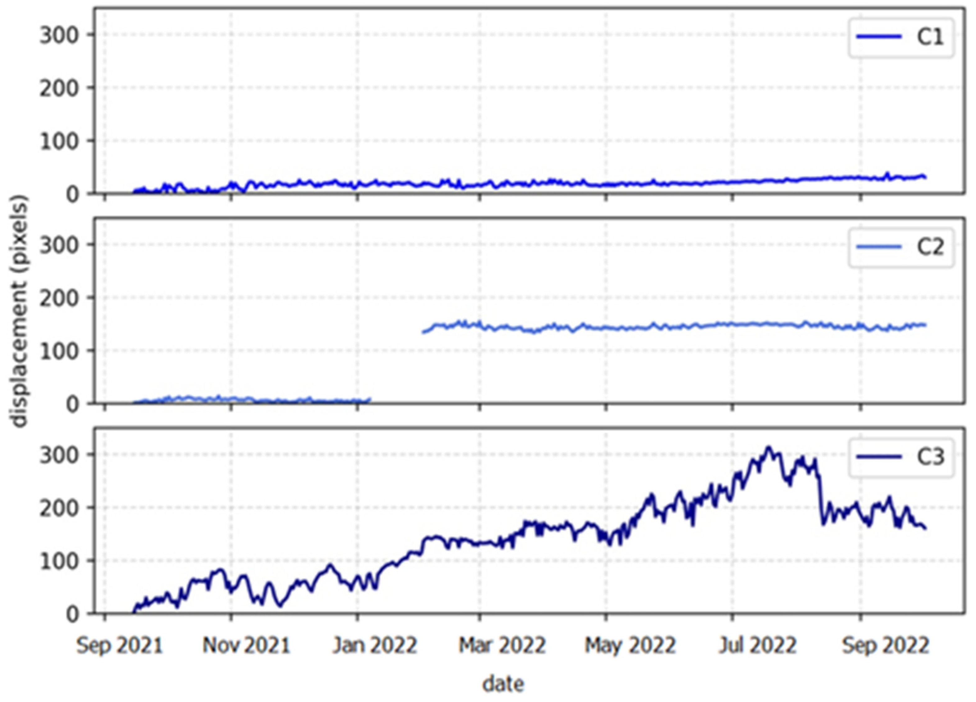
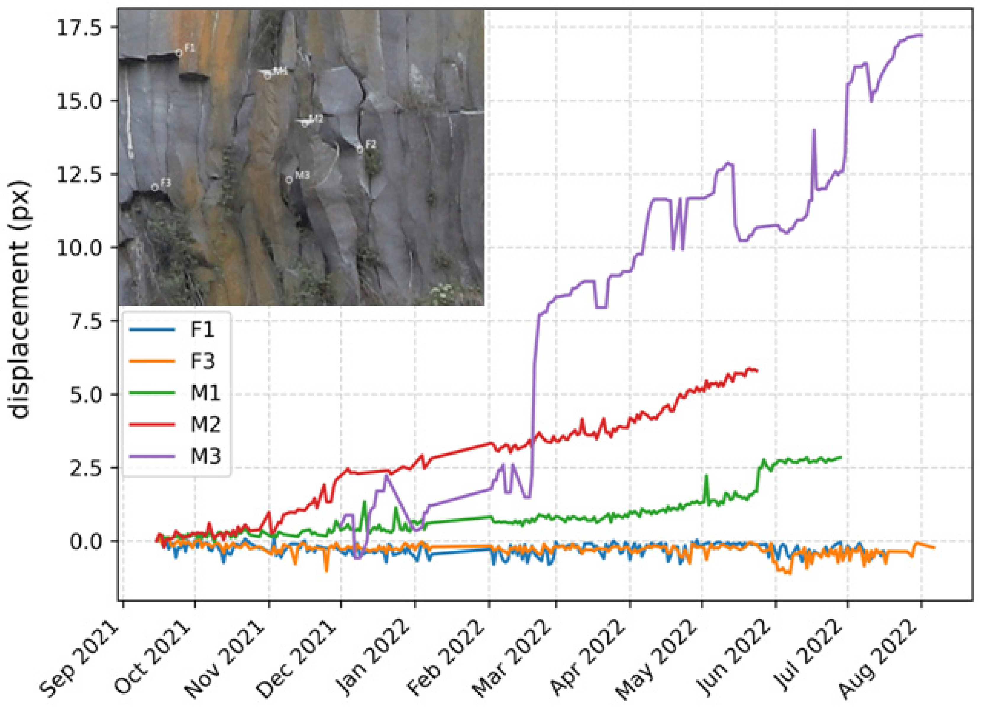
3. Results and Discussion
4. Conclusions
Author Contributions
Funding
Data Availability Statement
Acknowledgments
Conflicts of Interest
References
- Cruden, D.M.; Varnes, D.J. Landslide Types and Processes. In Landslides—Investigation and Mitigation; Transportation Research Board Special Report, No.247; Turner, A.T., Schuster, R.L., Eds.; National Academy of Sciences: Washington, DC, USA, 1996. [Google Scholar]
- Hungr, O.; Leroueil, S.; Picarelli, L. The Varnes Classification of Landslide Types, an Update. Landslides 2014, 11, 167–194. [Google Scholar] [CrossRef]
- Hoek, E. (Ed.) Analysis of Rockfall Hazards. In Practical Rock Engineering; RockScience: Toronto, ON, Canada, 2007; pp. 115–136. Available online: https://static.rocscience.cloud/assets/resources/learning/hoek/Practical-Rock-Engineering-Chapter-9-Analysis-of-Rockfall-Hazards.pdf (accessed on 17 November 2022).
- Corominas, J. Los Desprendimientos Rocosos, Impacto y Análisis Cuantitativo Del Riesgo. In Proceedings of the X Simposio Nacional sobre Taludes y Laderas Inestables, Granada, Spain, 13–16 September 2022; Hürlimann, M., Pinyol, N.M., Eds.; pp. 35–67. [Google Scholar]
- Coe, J.A. Bellwether Sites for Evaluating Changes in Landslide Frequency and Magnitude in Cryospheric Mountainous Terrain: A Call for Systematic, Long-Term Observations to Decipher the Impact of Climate Change. Landslides 2020, 17, 2483–2501. [Google Scholar] [CrossRef]
- Savi, S.; Comiti, F.; Strecker, M.R. Pronounced Increase in Slope Instability Linked to Global Warming: A Case Study from the Eastern European Alps. Earth Surf. Process. Landforms 2021, 46, 1328–1347. [Google Scholar] [CrossRef]
- Ruiz-Carulla, R.; Corominas, J.; Mavrouli, O. A Methodology to Obtain the Block Size Distribution of Fragmental Rockfall Deposits. Landslides 2015, 12, 815–825. [Google Scholar] [CrossRef] [Green Version]
- Albarelli, D.S.N.A.; Mavrouli, O.C.; Nyktas, P. Identification of Potential Rockfall Sources Using UAV-Derived Point Cloud. Bull. Eng. Geol. Environ. 2021, 80, 6539–6561. [Google Scholar] [CrossRef]
- Santana, D.; Corominas, J.; Mavrouli, O.; Garcia-Sellés, D. Magnitude-Frequency Relation for Rockfall Scars Using a Terrestrial Laser Scanner. Eng. Geol. 2012, 144–145, 50–64. [Google Scholar] [CrossRef]
- Blanch, X.; Eltner, A.; Guinau, M.; Abellan, A. Workflow for Enhanced Change Detection Using Time-Lapse Cameras. Remote Sens. 2021, 13, 1460. [Google Scholar] [CrossRef]
- Tonini, M.; Abellan, A. Rockfall Detection from Terrestrial Lidar Point Clouds: A Clustering Approach Using R. J. Spat. Inf. Sci. 2014, 8, 95–110. [Google Scholar] [CrossRef]
- van Veen, M.; Hutchinson, D.J.; Kromer, R.; Lato, M.; Edwards, T. Effects of Sampling Interval on the Frequency—Magnitude Relationship of Rockfalls Detected from Terrestrial Laser Scanning Using Semi-Automated Methods. Landslides 2017, 14, 1579–1592. [Google Scholar] [CrossRef]
- Williams, J.G.; Rosser, N.J.; Hardy, R.J.; Brain, M.J.; Afana, A.A. Optimising 4-D Surface Change Detection: An Approach for Capturing Rockfall Magnitude-Frequency. Earth Surf. Dyn. 2018, 6, 101–119. [Google Scholar] [CrossRef]
- Guerin, A.; Stock, G.M.; Radue, M.J.; Jaboyedoff, M.; Collins, B.D.; Matasci, B.; Avdievitch, N.; Derron, M.H. Quantifying 40 years of Rockfall Activity in Yosemite Valley with Historical Structure-from-Motion Photogrammetry and Terrestrial Laser Scanning. Geomorphology 2020, 356, 107069. [Google Scholar] [CrossRef]
- Hantz, D. Quantitative Assessment of Diffuse Rock Fall Hazard along a Cliff Foot. Nat. Hazards Earth Syst. Sci. 2011, 11, 1303–1309. [Google Scholar] [CrossRef] [Green Version]
- Corominas, J.; Matas, G.; Ruiz, R. Quantitative Analysis of Risk from Fragmental Rockfalls. Landslides 2019, 16, 5–21. [Google Scholar] [CrossRef] [Green Version]
- Carlà, T.; Nolesini, T.; Solari, L.; Rivolta, C.; Dei Cas, L.; Casagli, N. Rockfall Forecasting and Risk Management along a Major Transportation Corridor in the Alps through Ground-Based Radar Interferometry. Landslides 2019, 16, 1425–1435. [Google Scholar] [CrossRef] [Green Version]
- Feng, L.; Intrieri, E.; Pazzi, V.; Gigli, G.; Tucci, G. A Framework for Temporal and Spatial Rockfall Early Warning Using Micro-Seismic Monitoring. Landslides 2021, 18, 1059–1070. [Google Scholar] [CrossRef]
- Ulivieri, G.; Vezzosi, S.; Farina, P.; Meier, L. On the Use of Acoustic Records for the Automatic Detection and Early Warning of Rockfalls. In Proceedings of the 2020 International Symposium on Slope Stability in Open Pit Mining and Civil Engineering, Perth, WA, Australia, 12–14 May 2020; pp. 1193–1202. [Google Scholar] [CrossRef]
- Prades-Valls, A.; Corominas, J.; Lantada, N.; Matas, G.; Núñez-Andrés, M.A. Capturing Rockfall Kinematic and Fragmentation Parameters Using High-Speed Camera System. Eng. Geol. 2022, 302, 106629. [Google Scholar] [CrossRef]
- Noël, F.; Jaboyedoff, M.; Caviezel, A.; Hibert, C.; Bourrier, F.; Malet, J.-P. Rockfall Trajectory Reconstruction: A Flexible Method Utilizing Video Footage and High-Resolution Terrain Models. Earth Surf. Dyn. Discuss. 2022, 10, 1141–1164. [Google Scholar] [CrossRef]
- Matas, G.; Parras, E.; Lantada, N.; Gili, J.; Ruiz-Carulla, R.; Corominas, J.; Moya, J.; Prades, A.; Buill, F.; Nuñez-Andres, M.A.; et al. Laboratory Test to Study the Effect of Comminution in Rockfalls. In Proceedings of the XIII International Symposium on Landslides, Cartagena de Indias, Cartagena, Colombia, 22–26 February 2021; pp. 1–8. [Google Scholar]
- Ettore, D.; Anna, G.; Klaus, G.; Stephen, T.; Olivier, F. On the Dynamic Fragmentation of Rock—Like Spheres: Insights into Fragment Distribution and Energy Partition. Rock Mech. Rock Eng. 2022. [Google Scholar] [CrossRef]
- Dietze, M.; Mohadjer, S.; Turowski, J.; Ehlers, T.; Hovius, N. Validity, Precision and Limitations of Seismic Rockfall Monitoring. Earth Surf. Dynam. 2017, 12, 1–23. [Google Scholar] [CrossRef]
- Saló, L.; Corominas, J.; Lantada, N.; Matas, G.; Prades, A.; Ruiz-Carulla, R. Seismic Energy Analysis as Generated by Impact and Fragmentation of Single-Block Experimental Rockfalls. J. Geophys. Res. Earth Surf. 2018, 123, 1450–1478. [Google Scholar] [CrossRef] [Green Version]
- Janeras, M.; Jara, J.; Royan, M.; Vilaplana, J.M.; Aguasca, A.; Fabregas, F.; Gili, J.; Buxó, P. Multi-Technique Approach to Rockfall Monitoring in the Montserrat Massif (Catalonia, NE Spain). Eng. Geol. 2017, 219, 4–20. [Google Scholar] [CrossRef] [Green Version]
- Jaboyedoff, M.; Oppikofer, T.; Abellán, A.; Derron, M.H.; Loye, A.; Metzger, R.; Pedrazzini, A. Use of LIDAR in Landslide Investigations: A Review. Nat. Hazards 2012, 61, 5–28. [Google Scholar] [CrossRef] [Green Version]
- Royán, M.J.; Abellán, A.; Vilaplana, J.M. Progressive Failure Leading to the 3 December 2013 Rockfall at Puigcercós Scarp (Catalonia, Spain). Landslides 2015, 12, 585–595. [Google Scholar] [CrossRef]
- Eltner, A.; Kaiser, A.; Abellan, A.; Schindewolf, M. Time Lapse Structure-from-Motion Photogrammetry for Continuous Geomorphic Monitoring. Earth Surf. Process. Landforms 2017, 42, 2240–2253. [Google Scholar] [CrossRef]
- Westoby, M.J.; Brasington, J.; Glasser, N.F.; Hambrey, M.J.; Reynolds, J.M. “Structure-from-Motion” Photogrammetry: A Low-Cost, Effective Tool for Geoscience Applications. Geomorphology 2012, 179, 300–314. [Google Scholar] [CrossRef] [Green Version]
- Wang, X.; Frattini, P.; Stead, D.; Sun, J.; Liu, H.; Valagussa, A.; Li, L. Dynamic Rockfall Risk Analysis. Eng. Geol. 2020, 272, 105622. [Google Scholar] [CrossRef]
- Janeras, M.; Pedraza, O.; Lantada, N.; Núñez-Andrés, M.; Hantz, D.; Palau, J. TLS- and Inventory-Based Magnitude—Frequency Relationship for Rockfall in Montserrat and Castellfollit de La Roca. In Proceedings of the 5th RSS Rock Slope Stability Symposium, Chambéry, France, 13–15 November 2021; pp. 27–28. [Google Scholar]
- Abellán, A.; Jaboyedoff, M.; Oppikofer, T.; Vilaplana, J.M. Detection of Millimetric Deformation Using a Terrestrial Laser Scanner: Experiment and Application to a Rockfall Event. Nat. Hazards Earth Syst. Sci. 2009, 9, 365–372. [Google Scholar] [CrossRef] [Green Version]
- Abellán, A.; Vilaplana, J.M.; Calvet, J.; García-Sellés, D.; Asensio, E. Rockfall Monitoring by Terrestrial Laser Scanning—Case Study of the Basaltic Rock Face at Castellfollit de La Roca (Catalonia, Spain). Nat. Hazards Earth Syst. Sci. 2011, 11, 829–841. [Google Scholar] [CrossRef] [Green Version]
- Gance, J.; Malet, J.P.; Dewez, T.; Travelletti, J. Target Detection and Tracking of Moving Objects for Characterizing Landslide Displacements from Time-Lapse Terrestrial Optical Images. Eng. Geol. 2014, 172, 26–40. [Google Scholar] [CrossRef]
- Giacomini, A.; Thoeni, K.; Santise, M.; Diotri, F.; Booth, S.; Fityus, S.; Roncella, R. Temporal-Spatial Frequency Rockfall Data from Open-Pit Highwalls Using a Low-Cost Monitoring System. Remote Sens. 2020, 12, 2459. [Google Scholar] [CrossRef]
- Kromer, R.; Walton, G.; Gray, B.; Lato, M.; Group, R. Development and Optimization of an Automated Fixed-Location Time Lapse Photogrammetric Rock Slope Monitoring System. Remote Sens. 2019, 11, 1890. [Google Scholar] [CrossRef] [Green Version]
- Matas, G.; Prades-Valls, A.; Núñez-Andrés, M.A.; Buill, F.; Lantada, N. Implementation of a Fixed-Location Time Lapse Photogrammetric Rock Slope Monitoring System in Castellfollit de La Roca, Spain. In Proceedings of the 5th Joint International Symposium on Deformation Monitoring (JISDM), Valencia, Spain, 6–8 April 2022; p. 8. [Google Scholar]
- Buill, F.; Núñez-Andrés, M.A.; Rodríguez Jordana, J.J. Fotogrametría Arquitectónica; Fotogrametría Arquitectónica: Barcelona, Spain, 2005; ISBN 9788498803419. [Google Scholar]
- Desrues, M.; Malet, J.P.; Brenguier, O.; Point, J.; Stumpf, A.; Lorier, L. TSM-Tracing Surface Motion: A Generic Toolbox for Analyzing Ground-Based Image Time Series of Slope Deformation. Remote Sens. 2019, 11, 2189. [Google Scholar] [CrossRef] [Green Version]
- Lowe, D.G. Distinctive Image Features from Scale-Invariant Keypoints. Int. J. Comput. Vis. 2004, 60, 91–110. [Google Scholar] [CrossRef]
- Anders, N.; Valente, J.; Masselink, R.; Keesstra, S. Comparing Filtering Techniques for Removing Vegetation from Uav-Based Photogrammetric Point Clouds. Drones 2019, 3, 61. [Google Scholar] [CrossRef]
- Núñez-Andrés, M.; Prades-Valls, A.; Buill, F. Vegetation Filtering Using Colour for Monitoring Applications from Photogrammetric Data. In Proceedings of the 7th International Conference on Geographical Information Systems Theory, Applications and Management, Virtual, 23–25 April 2021. [Google Scholar]
- Paar, C.; Pelzl, J.; Preneel, B. Understanding Cryptography: A Textbook for Students and Practitioners; Springer: Berlin/Heidelberg, Germany, 2012; ISBN 3-642-04100-0. [Google Scholar]
- Lerma García, J. Fotogrametría Moderna: Analítica y Digital; Universitat Politècnica de València: Valencia, Spain, 2002; ISBN 8497052102. [Google Scholar]


| Real Displacement (H; D) cm | Horizontal Displacement Measured (H) cm | Discrepancies (H) cm | Depth Displacement Measured (D) cm | Discrepancies (D) cm |
|---|---|---|---|---|
| 0; 0 | 0.0 | 0 | 0.5 | 0.5 |
| 2; 2 | 2.0 | 0 | 2.5 | 0.5 |
| 5; 5 | 5.0 | 0 | 5.3 | 0.3 |
| 10; 10 | 9.7 | 0.3 | 10.4 | 0.4 |
| 0; 20 | --- | --- | 18.7 | 1.3 |
| X (m) | Y (m) | Z (m) | D (m) | |
|---|---|---|---|---|
| F1 | 0.008 | 0.050 | 0.025 | 0.040 |
| F2 | 0.006 | 0.026 | 0.007 | 0.028 |
| F3 | 0.015 | 0.025 | 0.017 | 0.033 |
| M1 | −0.275 | −0.262 | −0.065 | 0.385 |
| M2 | −0.106 | −0.217 | −0.088 | 0.257 |
| M3 | −.079 | −0.230 | −0.301 | 0.386 |
Disclaimer/Publisher’s Note: The statements, opinions and data contained in all publications are solely those of the individual author(s) and contributor(s) and not of MDPI and/or the editor(s). MDPI and/or the editor(s) disclaim responsibility for any injury to people or property resulting from any ideas, methods, instructions or products referred to in the content. |
© 2023 by the authors. Licensee MDPI, Basel, Switzerland. This article is an open access article distributed under the terms and conditions of the Creative Commons Attribution (CC BY) license (https://creativecommons.org/licenses/by/4.0/).
Share and Cite
Núñez-Andrés, M.A.; Prades-Valls, A.; Matas, G.; Buill, F.; Lantada, N. New Approach for Photogrammetric Rock Slope Premonitory Movements Monitoring. Remote Sens. 2023, 15, 293. https://doi.org/10.3390/rs15020293
Núñez-Andrés MA, Prades-Valls A, Matas G, Buill F, Lantada N. New Approach for Photogrammetric Rock Slope Premonitory Movements Monitoring. Remote Sensing. 2023; 15(2):293. https://doi.org/10.3390/rs15020293
Chicago/Turabian StyleNúñez-Andrés, Mª Amparo, Albert Prades-Valls, Gerard Matas, Felipe Buill, and Nieves Lantada. 2023. "New Approach for Photogrammetric Rock Slope Premonitory Movements Monitoring" Remote Sensing 15, no. 2: 293. https://doi.org/10.3390/rs15020293