Article

A Retrospective Analysis of National-Scale Agricultural Development in Saudi Arabia from 1990 to 2021

Climate and Livability Initiative, Division of Biological and Environmental Sciences and Engineering, King Abdullah University of Science and Technology (KAUST), Thuwal 23955-6900, Saudi Arabia
*
Author to whom correspondence should be addressed.
Remote Sens. 2023, 15(3), 731; https://doi.org/10.3390/rs15030731
Submission received: 7 November 2022 / Revised: 4 January 2023 / Accepted: 12 January 2023 / Published: 26 January 2023
(This article belongs to the Special Issue Monitoring Crops and Rangelands Using Remote Sensing)

Abstract

:
Agricultural intensification has resulted in the depletion of groundwater resources in many regions of the world. A prime example is Saudi Arabia, which witnessed dramatic agricultural expansion since the 1970s. To explore the influence of policy interventions aimed to better manage water resources, accurate information on the changes in the number and acreage of center-pivot fields is required. To quantify these metrics, we apply a hybrid machine learning framework, consisting of Density-Based Spatial Clustering of Applications with Noise, Convolutional Neural Networks, and Spectral Clustering, to the annual maximum Normalized Differential Vegetation Index maps obtained from Landsat imagery collected between 1990 to 2021. When evaluated against more than 28,000 manually delineated fields, the approach demonstrated producer’s accuracies ranging from 83.7% to 94.8% and user’s accuracies ranging from 90.2% to 97.9%. The coefficient of determination ( R 2 ) between framework-delineated and manually delineated fields was higher than 0.97. Nationally, we found that most fields pre-dated 1990 (covering 8841 km 2 in that year) and were primarily located within the central regions covering Hail, Qassim, Riyadh, and Wadi ad-Dawasir. A small decreasing trend in field acreage was observed for the period 1990–2010. However, by 2015, the acreage had increased to approximately 33,000 fields covering 9310 km 2 . While a maximum extent was achieved in 2016, recent decreases have seen levels return to pre-1990 levels. The gradual decrease between 1990 to 2010 was related to policy initiatives designed to phase-out wheat, while increases between 2010 to 2015 were linked to fodder crop expansion. There is evidence of an agricultural uptick starting in 2021, which is likely in response to global influences such as the COVID-19 pandemic or the conflict in Ukraine. Overall, this work offers the first detailed assessment of long-term agricultural development in Saudi Arabia, and provides important insights related to production metrics such as crop types, crop water consumption, and crop phenology and the overarching impacts of agricultural policy interventions.

1. Introduction

At the global scale, agricultural irrigation is responsible for up to 70% of freshwater withdrawals [1]. An even larger proportion is often required in arid countries to meet food production needs. Indeed, it was estimated that the agricultural sector consumes around 88% of freshwater withdrawals in Saudi Arabia, most of which are derived from non-renewable fossil groundwater that has remained sealed in an aquifer for tens of thousands of years or more due to changes in the surrounding geology [2,3]. Much of this unsustainable water use was the unintended consequence of a series of agricultural development plans (released every 5 years since the 1970s) that aimed to increase food self-sufficiency, improve individual livelihoods, diversify sources of national income, and reduce the dependence on oil. As a result of these sector-based initiatives, the area of irrigated agriculture in Saudi Arabia increased from less than 4000 km 2 before the 1970s to more than double that amount in the early 1990s [4]. An unfortunate but direct impact of these policies was the 60% decline in non-renewable water over the 25 years from 1979 to 2004 (The Eighth Development Plan 2005–2009) [5]. In later years, several policies were initiated to reduce the unsustainable water consumption, particularly via the reduction in subsidies related to the purchase price of wheat (The Fourth Development Plan 1985–1990) [6], reducing the wheat production by 6.9% annually from 1990 to 1995 (The Fifth Development Plan 1990–1995) [7], limiting wheat production so as not to exceed local consumption, and encouraging the production of high-value crops requiring less water (The Sixth Development Plan 1995–2000) [8]. Specifically, The Eighth Development Plan 2005–2009 [5] emphasized that high levels of self-sufficiency would no longer be a strategic objective. Consequently, the expansion of agricultural lands was suspended for five years in 2003, the export of wheat was banned, and the export of vegetables cultivated on open fields was prevented for five years (Council of Ministers Resolution No.335 of 2007). However, with farmers replacing wheat with alfalfa, the water management objective was not fully realized [9]. Additional policy initiatives were implemented since 2010 to seek a more sustainable way to balance the challenging water- and food-security issues, exemplified through the “National Water Strategy 2030” [10]. Examples include promoting the cultivation of fruit trees that are suited for the Kingdom’s environment, such as olive trees in Al Jawf (The Ninth Development Plan 2010–2014) [11], and reducing the non-renewable groundwater consumption in the agricultural sector from 17 billion m 3 in 2016 to 9 billion m 3 in 2020 (Saudi Vision 2030) [12].
The agricultural expansion witnessed during the 1990s resulted from the construction of vast numbers of center-pivot systems, which were irrigating two-thirds of the agricultural land in Saudi Arabia by the early 2000s [13,14]. Given the predominance of this system, mapping the patterns of field growth and decline is required to provide insights into the agricultural development in Saudi Arabia, especially for quantifying crop water consumption [15]. Interestingly, although there were considerable policy interventions and other changes occurring throughout the agricultural sector over the last three decades, no study has yet cataloged the most direct measures of sector productivity: the field number and extent. Satellite imagery has proven to be an optimal solution for large scale agricultural mapping, as it often represents the only viable data source for retrospective detection in this region [16,17,18,19].
There are three main methodologies for center-pivot field detection using satellite imagery. First, the manual interpretation of imagery—whereby individual field masks are identified and mapped—is favoured for small regions, but is limited due to the intensive labor requirement [20,21,22]. Second, the development of image segmentation methods allowed for the semi-automated delineation of agricultural fields for larger regions, making it a popular methodology [23,24,25,26]. Some image segmentation methods used for field delineation included (a) edge-based techniques that detect pixels on the field boundaries, e.g., Canny detection [27]; (b) regional-based techniques in which objects are obtained by grouping pixels based on the homogeneity criterion, among which watershed segmentation and multi-resolution segmentation are the most frequently employed methods [28,29]; and (c) shaped-based techniques utilizing the shape information for image segmentation, e.g., the Hough transformation [30,31]. Finally, and most recently, machine learning, especially deep learning techniques, has become the state of the art for identifying and delineating field boundaries [32,33,34], with convolutional neural networks (CNNs) [35] becoming the predominant tool for this task.
From the machine learning perspective, Zhang et al. [36] first explored the implementation of CNNs for center-pivot field detection using three techniques, LeNet, Alexnet, and VGGnet [37,38,39], and used these to detect the central location of fields successfully. Since then, more advanced CNNs were utilized to mask the extent or identify the boundary of center-pivot fields, including fully convolutional networks (e.g., U-net) [40,41,42] and instance segmentation methods such as Mask-RCNNs that utilize region-based CNNs [16,43,44]. However, implementing a single machine learning technique often has limitations, including an inability to segment satellite imagery into individual field objects and the considerable burden of producing or obtaining suitable training data. Such limitations can be overcome by applying a hybrid framework consisting of multiple machine learning algorithms or by combining machine learning algorithms with other segmentation methods [45,46]. As an example, Li et al. [47] proposed a hybrid framework consisting of three machine learning techniques, the Density-Based Spatial Clustering of Applications with Noise (DBSCAN), CNNs, and spectral clustering, to delineate fields in an agricultural region in the north of Saudi Arabia. The framework achieved high accuracies when evaluated against more than 4000 manually delineated fields: 97 and 98% of the object-based producer’s and user’s accuracies, respectively. However, in that case, the evaluation was performed within a single agricultural region in Saudi Arabia, with the performance in other regions and periods not considered.
The overall objectives of this paper focus on efforts to (1) implement the hybrid framework proposed in Li et al. [47] and evaluate its performance to other agricultural regions across Saudi Arabia and (2) apply the approach to delineate the center-pivot fields in the main agricultural regions in Saudi Arabia using a three-decades-long time series of Landsat data, i.e., from 1990 to 2021. A key motivation of this work was not only to obtain the boundary of the center-pivot fields, but also to quantify the agricultural dynamics and provide the baseline information needed for parallel agricultural-related investigations. The agricultural dynamics included the variation in the total number and extent, the size distribution, and the first and last detection year of the center-pivot fields from 1990 to 2021. The field acreage dynamics can provide a straightforward indicator of where and when farmers and agricultural companies implemented the government policy initiatives. The analysis can also be used to infer the variations in the groundwater use across the agricultural sector, because fields are mainly irrigated using non-renewable groundwater [2]. With the foundation provided by this work, higher-level studies can be launched using these data, with examples including the crop type discrimination and crop yield estimation [48,49], crop phenology description [50], and crop water consumption estimation [15,51].

2. Study Site and Data Description

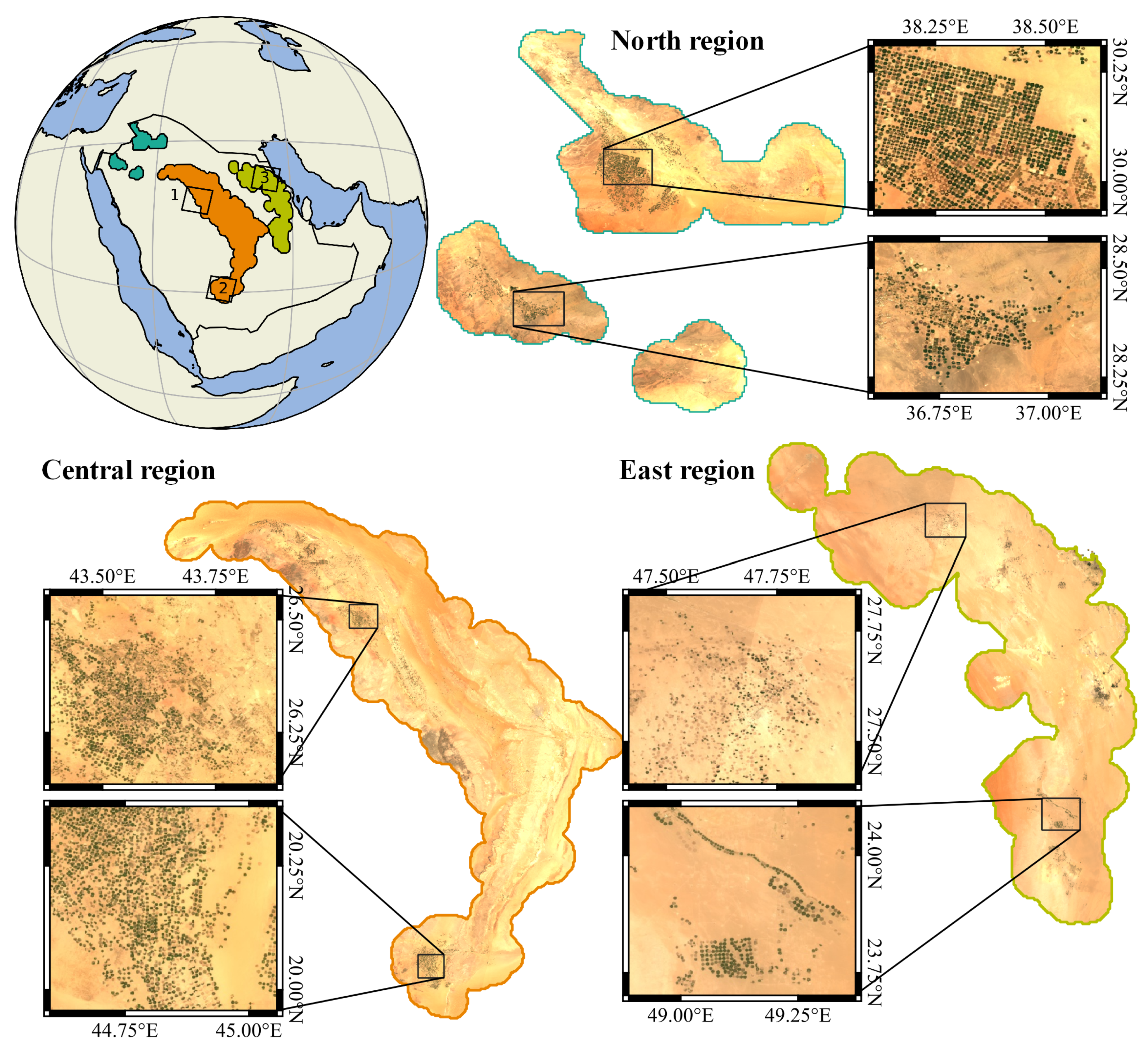
2.1. Study Site: The Main Agricultural Regions in Saudi Arabia

Located between latitudes 15 22 N and 32 09 N and longitudes 34 50 E and 55 50 E, Saudi Arabia occupies around 80% of the Arabian Peninsula. With annual rainfalls averaging 100–120 mm/year (mainly from October to May) and daily maximum temperatures exceeding 45 C during the summer months, Saudi Arabia is one of the driest regions worldwide [52]. Johansen et al. [53] determined that there were 11,555 km 2 of center-pivot fields distributed across Saudi Arabia in 2015, the majority with sizes ranging from 200 to 500 m in radius. That study focused on the main agricultural regions of Al Jawf, Tabuk, Ha’il, Al Qassim, Riyadh, Wadi ad-Dawasir, and the Eastern Province [53]. The dominant crops reported in the statistical yearbook 2019 were foraged crops (mainly alfalfa), cereals (mainly wheat, barley, and broom-corn), vegetables (mainly watermelon, potato, and tomato), and fruits (mainly dates, citrus, and grapes) [54]. In this study, the abovementioned administrative units were grouped into three major geographical regions: the north region (Tabuk and Al Jawf), the central region (Ha’il, Al Qassim, Riyadh, and Wadi ad-Dawasir), and the east region (agricultural regions within the Eastern Province) (Figure 1). Spatial variations between different regions were observed, including larger fields and more uniformity in the north and east regions and more variability in the field area and shapes in the central region [53]. Given the predominance of center-pivot systems (both circular and fan-shaped) operating within the agricultural fields of the Kingdom, these were the primary focus of analysis herein. That decision was also made in part due to the limitations of 30 m resolution Landsat pixels being able to accurately capture field boundaries. Furthermore, it is noted that the term “center-pivot fields” is often used interchangeably with “fields” throughout the text.

2.2. Landsat Data

Level-2 surface reflectance data from Landsat-4/5 Thematic Mapper, Landsat-7 Enhanced Thematic Mapper (ETM+), and Landsat-8 Operational Land Imager (OLI) for the period 1990 to 2021 were processed using the Google Earth Engine, a cloud-based platform capable of processing large amounts of geospatial data including the entire catalog of Landsat images [55]. Table 1 shows the total number of scenes processed per year for each of the three regions, representing a total of 14,695 images for the entire study. While Landsat data were only collected every five years prior to 2015 (to match the cycle of government development plans), they were analyzed every year since 2015 to capture the impacts of several recent policy instruments on the agricultural sector.
In line with earlier methodologies [47], the field delineation framework takes the annual maximum normalized difference vegetation index (NDVI) map as the base map, which was obtained from the maximum NDVI values of each pixel from up to 23 Landsat images in each target year. Without the large number of images wrmithin a single year, many fields would be omitted, as some fields are only active in use for short periods every year. NDVI was computed as
NDVI = NIR red NIR + red
where NIR and red represent the surface reflectance of the near-infrared and red bands, respectively. Areas within the Landsat images contaminated with cloud cover and cloud shadows produced low NDVI values and hence did not impact the generation of the annual maximum NDVI maps used in the machine learning framework. The maximum NDVI images were processed by the Google Earth Engine and then downloaded to a local machine for further processing.

2.3. Ground-Truth Data

Because the Li et al. [47] field delineation framework was only evaluated against ground-truth data from one region (Al Jawf), this study required further adaptation and evaluation for the other regions. Three Landsat tiles were selected to perform manual delineations, comprising paths/rows 165/41, 166/46, and 168/42. The location of the three tiles is shown in Figure 1 as numbered black rectangles. The manual delineation of fields on these three tiles was performed with the help of the annual maximum NDVI maps for the years 2000, 2010, and 2015. Landsat-8 was utilized for 2015, Landsat-7 for 2010, and both Landsat-7 and -5 for 2000. First, polygons masking each field on the annual maximum NDVI map were created. Then, fields with a median NDVI value less than 0.25 were eliminated from the ground-truth dataset, as they likely represent previously cultivated fields that were then left fallow. Table 2 shows the number of scenes utilized to perform the manual delineation. It is necessary to select the high number of manually delineated fields for validation, due to the large variation of field sizes, shapes, and density of the fields as well as surrounding landscape characteristics, varying management practices; seasonal and annual variation in growth patterns and crop types; and to include regions where fields have overlapping field edges. Given the span of Landsat platforms used, the field delineation framework’s performance when using different input data sources could also be evaluated, especially for the case of Landsat-7, which was impacted by the failure of the Scan Line Corrector from 31 May 2003, resulting in 22% of the data missing [56,57].

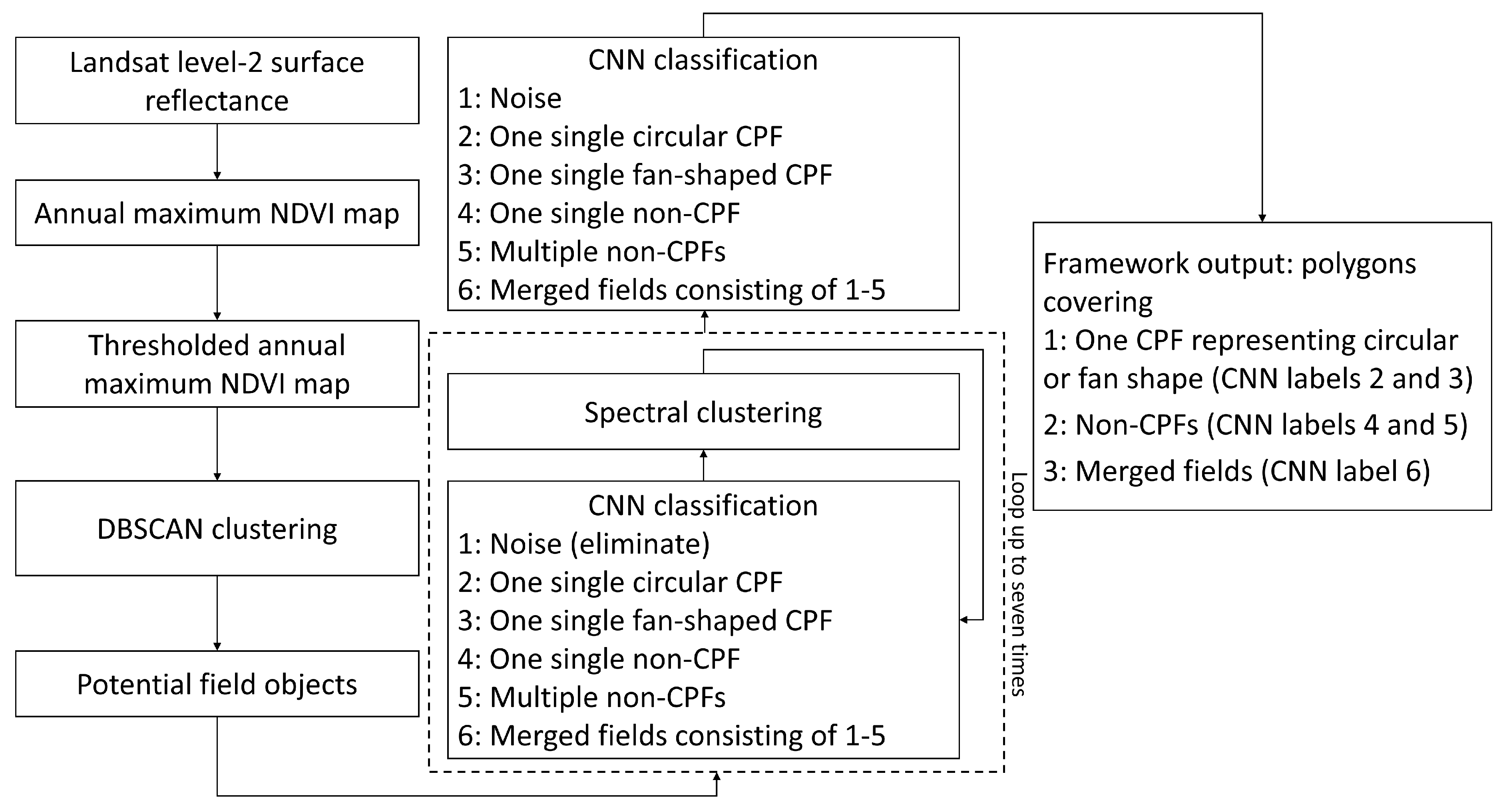
3. Field Delineation Framework

3.1. Framework Description

As the study by Li et al. [47] performed well when using different satellite data and produced a high object-based producer’s accuracy of 97% and user’s accuracy of 98% when assessed against 4000 manually identified fields, that framework was further explored herein. Revisiting that approach, three machine learning techniques, i.e., DBSCAN [58], CNNs classification [37], and spectral clustering [59] were operated in sequence herein to identify and delineate the center-pivot fields, with the schematic showing in Figure 2. The following provides a brief overview of the technique, with the reader directed to Li et al. [47] for a more detailed description of the hybrid machine learning framework. As a first step, the annual maximum NDVI map was obtained using NDVI maps calculated from Landsat Level-2 surface reflectance imagery for each target year. A thresholded NDVI map was obtained by eliminating pixels with NDVI values below a threshold value, i.e., 0.25 herein, which were mainly bare soil background pixels. Then, pixels from annual maximum NDVI maps were segmented into potential field objects using DBSCAN. The type of the field objects was further classified into six categories by a classic CNN approach, i.e., AlexNet, including circular center-pivot field (CPF), fan-shaped CPF, non-CPF (fields presenting rectangle shapes), multiple non-CPFs, merged fields, and noise. Next, the merged fields and multiple non-CPFs were re-clustered into individual fields by spectral clustering. The CNN classification and spectral clustering can be run up to seven iterations to cluster the multiple fields into individual fields or until no field object was identified as merged fields. Finally, polygons were created for each cluster representing individual field masks. We group both circular and fan-shaped fields as one in the final result because the shape of the field was not of interest in this study.
DBSCAN is an unsupervised classification method that clusters a dataset based on the density of data points. A benefit of DBSCAN is that it does not require the user to specify the number of clusters. Data points are classified as the core, border, and noise points according to two global parameters: the radius ( E p s ) for a point to search for its neighbors and the number of neighbors ( M i n P t s ) within E p s [60]. A cluster is defined as a set of data points such that the density of points within the cluster is higher than the density of points outside the cluster (a maximal set of density-connected points) [61]. DBSCAN was applied for tree crown segmentation [62], and woody component identification of trees [61] using LiDAR data. Its ability to segment agricultural fields was demonstrated recently by Li et al. [47].
CNN is an artificial neural network inspired by biological neural networks [63]. The nodes in the input layer, hidden layers, and output layer are connected by modeled weights, which are updated iteratively during the training stage to minimize the error between actual and predicted outputs [64]. AlexNet is one of the most classic and straightforward CNNs successfully applied to identify center-pivot fields using satellite imagery [36]. In this study, we used the AlexNet model detailed by Li et al. [47], which was trained using Landsat-8 images of Al Jawf (upper image in Figure 1) from 2018.
Spectral clustering is widely used for image segmentation [65,66]. It clusters data by a similarity graph, which is constructed by vertices representing data points, the edges between the vertices, and the weight of the edges [67]. In this study, weights were formed by the Gaussian kernel function of the difference in NDVI values from two adjacent pixels and were set to 0 for nonadjacent pixels [68]. The target of spectral clustering was to find the k smallest eigenvalues of eigenvectors for a Laplacian matrix formed by a degree matrix and weight matrix, where k is the number of clusters ( N c l u ) set by the user. Spectral clustering was run using a set of N c l u values. Finally, the Calinski-Harabasz index [69], which combines cohesion and separation of clustering results, was used to select the optimal N c l u value. More detailed information of the hybrid machine learning framework was described in Li et al. [47].

3.2. Evaluation Metrics

The framework’s performance was evaluated using the same metrics employed by Li et al. [47]. Herein, “framework-delineated fields” refers to fields that are delineated using the machine learning framework presented in Section 3.1, whereas “ground-truth fields” were manually delineated. Pixels with NDVI values of less than 0.25 were excluded from calculating these indices and when calculating the field acreage because we only focused on those with vegetation growth. A pixel with an annual maximum NDVI value of less than 0.25 was unlikely to be covered by vegetation during the year. This low NDVI filtering was required to exclude fallow areas within a field that result from certain irrigation application configurations (e.g., irrigating using only the outer sections of the pivot, which results in a donut shape). The evaluation metrics included the producer’s and user’s accuracies calculated on both object and pixel basis; the over- and under-segmentation error and intersection over union error ( S o v e r , S u n d e r and IoU error, respectively) on a pixel basis, which provide values ranging from 0 to 100%, with a value of 0 indicating a perfect delineation result and a value of 100% indicating a high degree of over- or under-segmentation error, and an incorrect delineation result, respectively; and the coefficient of determination ( R 2 ), the mean absolute error (MAE), and the relative mean bias deviation (rMBD) of the acreages between the framework-delineated fields and ground-truth fields. The number of ground-truth fields and framework-delineated fields was referred to as N t r u e and N e s t i , respectively (see Table 3). A framework-delineated field was defined as a correctly detected field (Table 3; N e s t i ( c ) ) if (1) the field was identified as a CPF by the CNN and (2) both the S o v e r and S u n d e r values did not exceed 40%. For a correctly detected field, it was defined as an over-segmented field if the S o v e r value was higher than 40%, and an under-segmented field if the S u n d e r value was higher than 40%. The number of over-segmented and under-segmented fields was referred to as N o v e r s e g and N u n d e r s e g in Table 3. A field was delineated correctly if both S o v e r and S u n d e r values did not exceed 40%, the number of which was computed as:
N d e l i ( c ) = N e s t i ( c ) N o v e r s e g N u n d e r s e g
The producer’s and user’s accuracy on the object basis (referred to as A c c u P r o d o b j and A c c u U s e r o b j ) was thus calculated as:
A c c u P r o d o b j = N d e l i ( c ) / N t r u e
A c c u U s e r o b j = N d e l i ( c ) / N e s t i
The pixel-basis producer’s and user’s accuracy (referred to as A c c u P r o d p x l and A c c u U s e r p x l ) was obtained as:
A c c u P r o d p x l = p i x e l s o f c o r r e c t l y d e l i n e a t e d f i e l d s p i x e l s o f g r o u n d t r u t h f i e l d s
A c c u U s e r p x l = p i x e l s o f c o r r e c t l y d e l i n e a t e d f i e l d s p i x e l s o f f r a m e w o r k d e l i n e a t e d f i e l d s
The number of fields that failed to be detected as CPFs was also counted, including CPFs detected as non-CPFs representing rectangle shapes (Table 3; N C P F 2 n o n C P F ) and undetected CPFs (Table 3; N o m i t ) defined as a union of CPFs (1) being identified as noise by the CNN, and thus excluded by the framework, (2) not intersected with any framework-delineated fields, or (3) with both the S o v e r and S u n d e r values higher than 40%, under which circumstances the framework-delineated field and ground-truth field were treated as two different fields. N o m i t was equivalent to:
N o m i t = N t r u e N e s t i ( c ) N C P F 2 n o n C P F

4. Results

The results of this study focused on two aspects, i.e., an evaluation of the field delineation framework against the ground-truth dataset (Section 4.1) and retrospective analysis of the field dynamics on a national scale in Saudi Arabia since 1990 (Section 4.2). The framework was assessed at both the object and pixel levels (Section 4.1.1), with potential causes of errors presented in Section 4.1.2. The field dynamics analysis focused on the changes in the field numbers and acreage in Section 4.2.1, the dynamics of the field size distribution in Section 4.2.2, and the field expansion and contraction dynamics in Section 4.2.3.

4.1. Evaluation of the Hybrid Machine Learning Framework Using Three Landsat Tiles

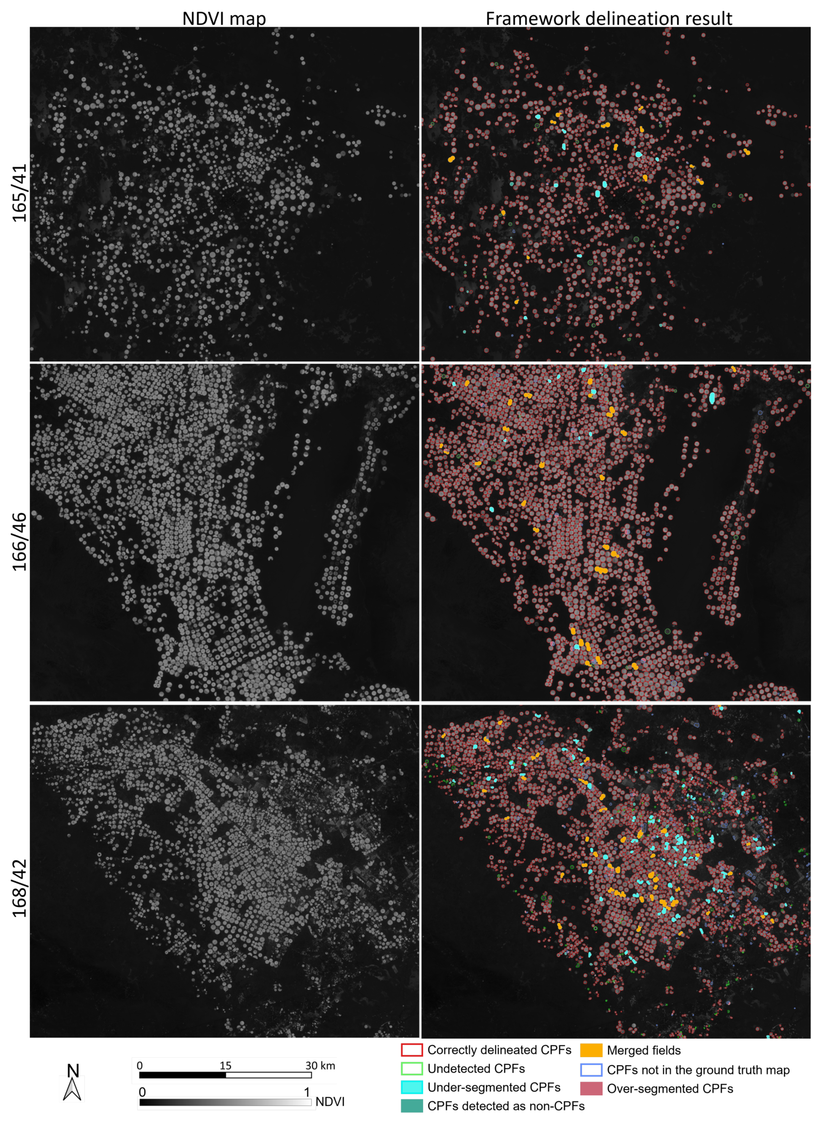
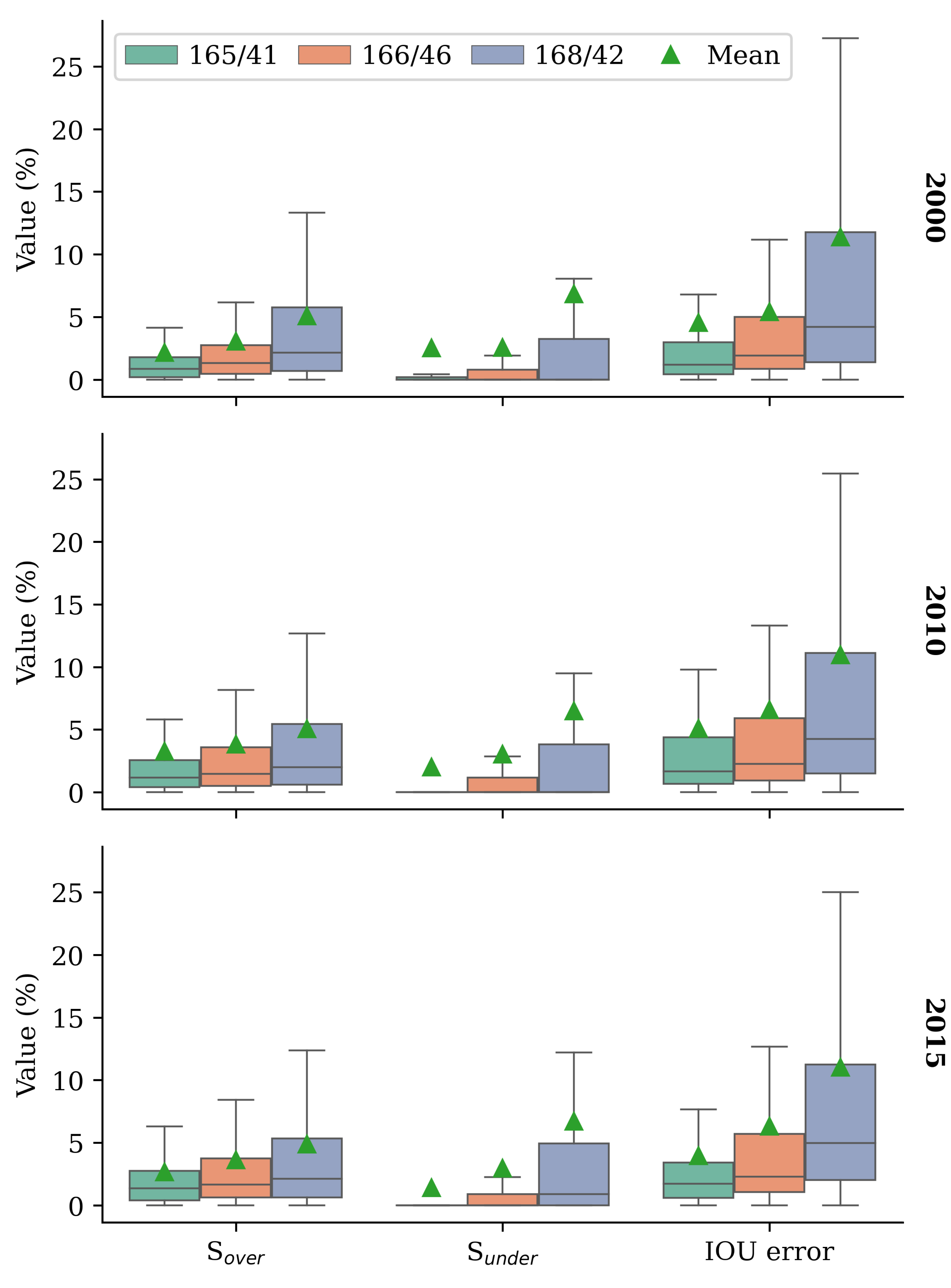
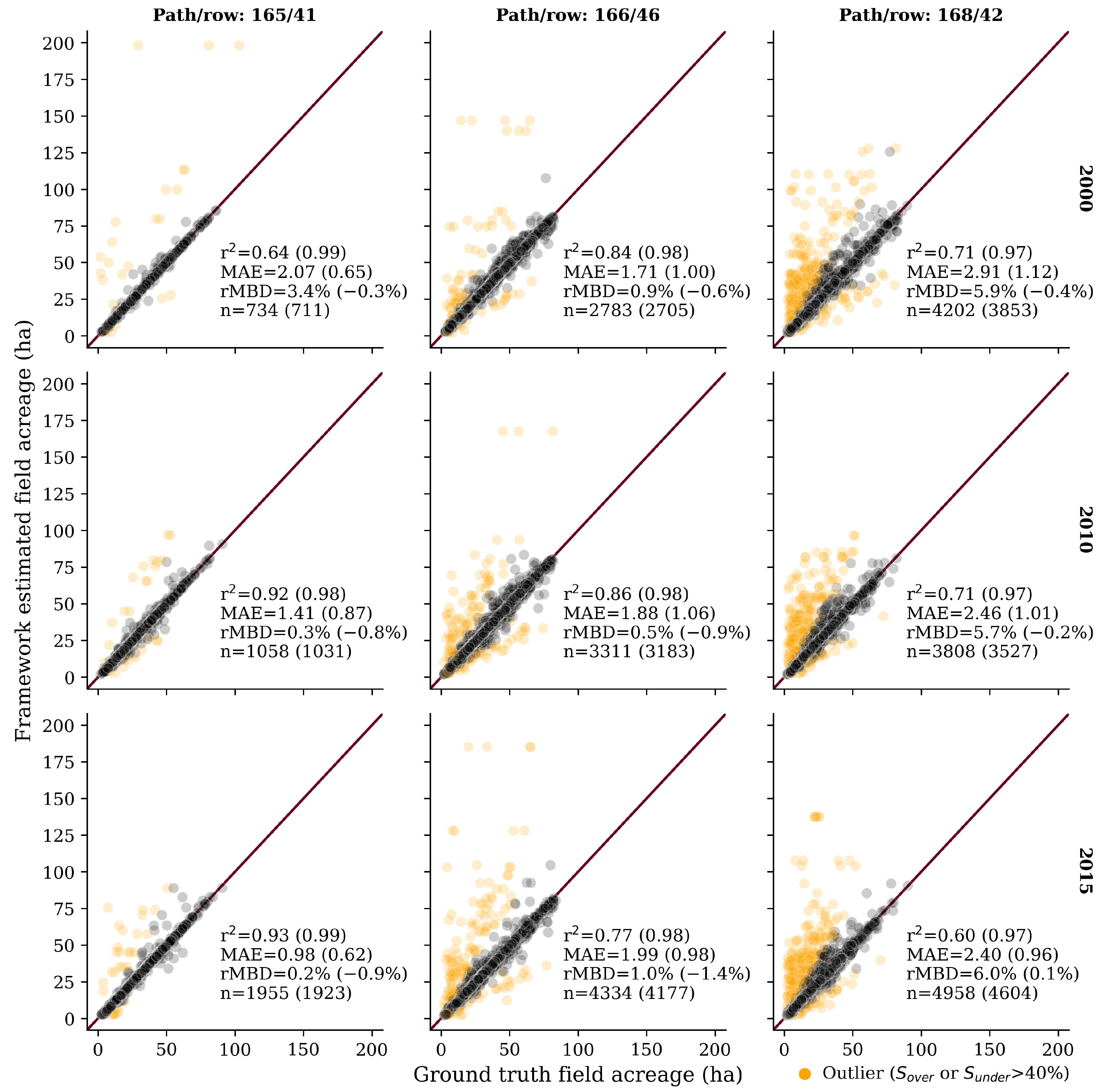
4.1.1. Accuracy of the Field Delineation Framework

The delineation results evaluated against the ground-truth data are shown in Figure 3 for the year 2015. Generally, the framework performed well across all of the three Landsat tiles from the different regions in Saudi Arabia (Figure 1). The producer’s and user’s accuracies at an object-level for 2015 were 93.7 and 97.9% for tile 165/41, 94.8 and 95.9% for tile 166/46, and 86.8 and 91.0% for tile 168/42, respectively (Table 3; rows 9 and 10). Three main types of delineation error were identified. The first type was the over- and under-segmentation of some fields (Table 3; rows 4 and 5, respectively). The under-segmentation occurred for some groups of multiple fields when the CNN incorrectly classified merged fields as a single field and when the spectral clustering approach failed to further segment “merged fields” that were correctly classified by the CNN. More fields in tile 168/42 were under-segmented than in the other two tiles (i.e., 5.3, 1.1, and 2.7% for tiles 168/42, 165/41, and 166/46, respectively), resulting in a lower accuracy for tile 168/42 (Table 3; rows 9 and 10). A second type of error was when the CNN misclassified a field as a non-center pivot, which occurred in up to 2.7% of the ground-truth center-pivot fields (Table 3; row 7). A third type was that some fields on the ground-truth map were not presented on the framework-delineated map (Table 3; row 8), which was up to 5.3% in 2015 and even higher in 2000 and 2010, resulting in lower accuracies for those years.
The delineation results were also assessed at the pixel level. The producer’s accuracy at the pixel level was generally higher than at the object level (Table 3) due to delineation errors being more likely to occur for small fields, resulting in a smaller proportion of pixels than the number of fields being identified incorrectly. The boxplots of the S o v e r , S u n d e r , and IoU error values for the three evaluation tiles are shown in Figure 4. In general, the delineation results showed low over- and under-segmentation errors. The median values of S o v e r , S u n d e r , and IoU error were less than 2.1, 0.9, and 5% for all the correctly detected fields (fields in Table 3; row 3). While the under-segmentation errors at the object level were higher than the over-segmentation errors, these indicated the number of fields with S o v e r or S u n d e r values exceeding 40% (Table 3; rows 4 and 5). In contrast, the over-segmentation errors at the pixel level were higher than the under-segmentation errors (Figure 4), suggesting that a framework-delineated field was more likely to be smaller instead of larger than the ground-truth field. The difference between the mean and median values of S u n d e r was higher than that of S o v e r , due to a larger number and magnitude of outliers for the S u n d e r values, i.e., more fields were being under-segmented, which was consistent with the object-based analysis. Tile 168/42 showed more segmentation errors than the other two tiles, which can be explained by the more complex agricultural parcel distributions in this region compared to the other two tiles, i.e., the central region contains a larger number of smaller, irregularly-shaped fields, with less spacing between them (Figure 3). Johansen et al. [53] also reported lower accuracies in this region compared to other regions in Saudi Arabia, albeit using a different object-based image analysis technique. Indeed, the complex field conditions played a more significant role than the data source, e.g., the data striping in Landsat-7 did not result in more fields being over-segmented in tile 168/42 in 2010 compared to 2015 (Figure 4 and Table 3).
The comparison of the acreage of individual ground-truth fields and framework-delineated fields is shown in Figure 5. The coefficient of determination ( R 2 ) ranged from 0.60 to 0.93 for different tiles and years when all the fields correctly detected by the framework were included (fields in Table 3; row 3). After eliminating the incorrectly delineated fields on the basis of being over- and under-segmented ( S o v e r > 40% or S u n d e r > 40%), i.e., keeping only fields in row (6) of Table 3, the R 2 values increased to a range from 0.97 to 0.99. Considering that the outliers represented less than 8% (tile 168/42) of the fields, the overall framework performed well. The scatterplots also show that more outliers were caused by under-segmented fields, resulting in the framework-delineated fields overestimating the field acreage (i.e., more outliers in the upper left corner of the scatterplots). However, after removing the outliers, the rMBD values were generally negative, which indicated that the framework tends to underestimate field acreage. That result suggests over-segmentation, which can be caused by either the presence of lower NDVI values (which were ignored by the framework and thus created false boundaries within a field) or by low NDVI pixel values along the real field boundary, thus shifting the real field boundary inwards.

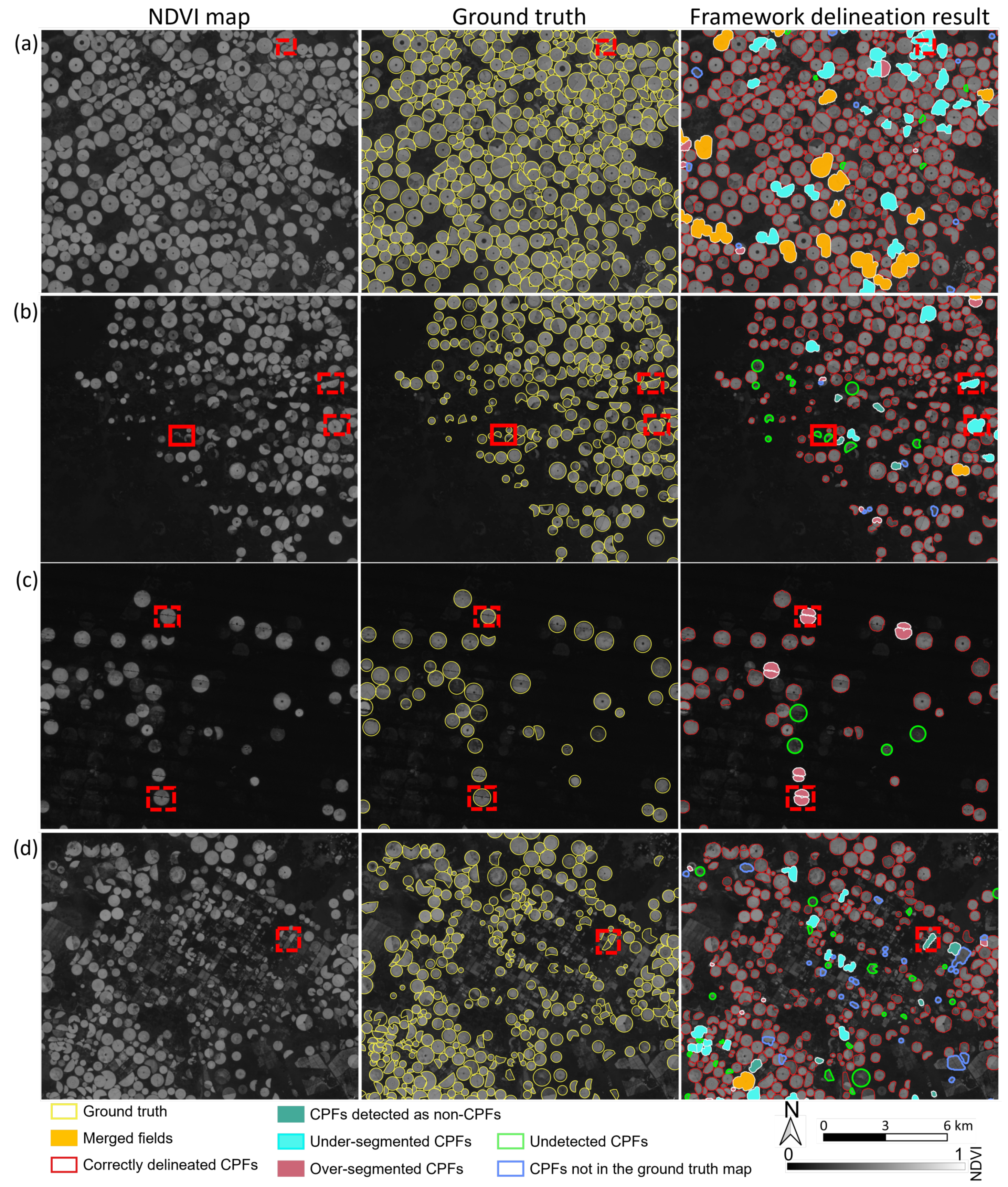
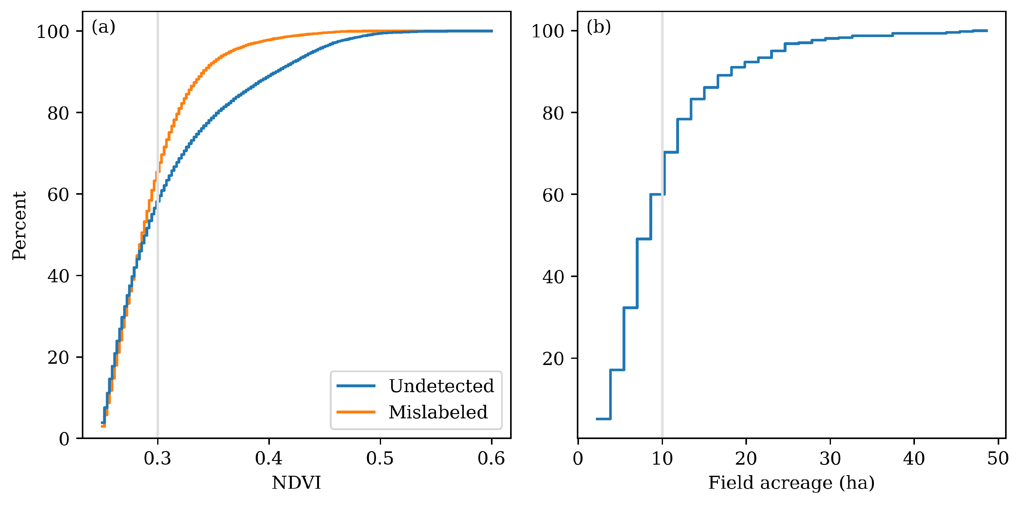
4.1.2. Error Interpretations

Some examples of delineation errors are shown in Figure 6. Two main issues caused the under-segmentation error: a field object which consisted of multiple fields was (1) classified by the CNN as a merged field, and (2) wrongly classified by the CNN as a single CPF. In the first case, the CNN approach classified the merged objects correctly. However, the framework showed limitations when segmenting these merged objects. Increasing the spatial resolution of the input satellite data, e.g., using Sentinel-2 imagery with a 10 m spatial resolution might reduce such errors. In the second case, the CNN approach classified the field objects into the wrong class, i.e., field objects that should have been classified as merged objects were instead classified as a single center-pivot field object. Thus, further re-clustering processing was not implemented. An example of this error is shown in the dashed red rectangle in Figure 6a, where two fan-shaped fields were close to each other. The outline of the two fields was similar to a circle and was identified as one circular field, resulting in an under-segmentation error. Another two under-segmentation error examples are shown in the dashed red rectangles in Figure 6b, where a field object that was classified as a single field consisted of a large field and a small field within the ground-truth map.
One of the causes of the over-segmentation error was the use of a larger cluster number to implement the spectral clustering on a field object consisting of multiple fields. The framework searched for the optimal cluster number within a list of candidates, which was computed based on the number of pixels forming a field with a diameter of 800 m. Although flexible upper and lower constraints were used to set the candidates, these may not work for fields with extremely small or large diameters. Another cause of the over-segmentation was that the CNN step classified a single field as multiple fields, and thus further re-clustering procedures were implemented to segment the field into several small sub-parts. In addition to these limitations, the striping pattern in the Landsat-7 images (due to the Scan Line Corrector failure) is likely another cause for the over-segmentation. For example, the five fields in Figure 6c (two examples are highlighted in the dashed red rectangles) were over-segmented due to the visible stripes in the annual maximum NDVI map, which resulted in a high NDVI gradient for the pixels affected by the data stripes. Thus, the fields were arranged into two clusters by either the DBSCAN or spectral clustering. Because Landsat-7 was the only data source in 2010 (Table 2), this might be the main reason why more fields were over-segmented in 2010 than in 2000 and 2015 for tiles 165/41 and 166/46 (Table 3). The effect of Landsat-7 image striping was offset by the use of Landsat-5 in 2000.
One key initial step within the framework was the accurate detection of fields (Table 3; row 8) with low NDVI values (see Figure 6b–d, an example was highlighted in the solid red rectangle in Figure 6b), which might cause an underestimation of the acreage of the fields with active crop production. The framework uses a thresholded NDVI value of 0.25 to filter the annual maximum NDVI map at the beginning of the processing, which is designed to exclude the pixels covering bare soil. Thus, if a field contained a significant fraction of low NDVI values, then the shape of the field could be misclassified (e.g., as a non-center-pivot field showing a rectangle shape), or the entire field could be classified as noise and excluded from the results entirely. Figure 7 suggests that approximately 60% of the NDVI values of the pixels within the center-pivot fields that were not detected-or detected as non-center-pivot fields by the framework-were smaller than 0.3. Another factor contributing to the center-pivot fields being identified as non-center-pivot fields was the field’s size, especially for the fan-shaped structures (light seagreen polygons in Figure 6b,d). Approximately 60% of the center-pivot fields detected as non-center-pivot fields were smaller than 10 ha (approximately 110 Landsat pixels, Figure 6c), which were significantly smaller than the majority of the fields that typically had diameters of around 500 m (or around 20 ha in area). As such, the 30 m spatial resolution of the Landsat imagery represents a limitation in correctly representing the shape of small fields. Multiple small center-pivot fields presenting fan shapes might be grouped and identified as a non-center-pivot field (dashed red rectangle in Figure 6d). On the other hand, the framework identified some of the non-center-pivot fields as center-pivot fields (Figure 6d; label “CPFs not in the ground truth map”) due to the classification errors made by the CNN.

4.2. Retrospective Center-Pivot Field Dynamics on a National Scale in Saudi Arabia since 1990

As detailed above, the framework generally performed well in delineating most of the fields. However, for some agricultural regions, where fields with irregular shapes were observed (e.g., Landsat tile 168/42), under-segmentation errors occurred. The majority of these under-segmented fields could be readily identified because some were classified as merged field objects while others were generally large objects on the field delineation maps. These field polygons were manually corrected to ensure high-accuracy delineation results at the national scale. As such, the retrospective results explored in this section included a small amount of manual correction, accounting for an average of 4.5% of the total fields.

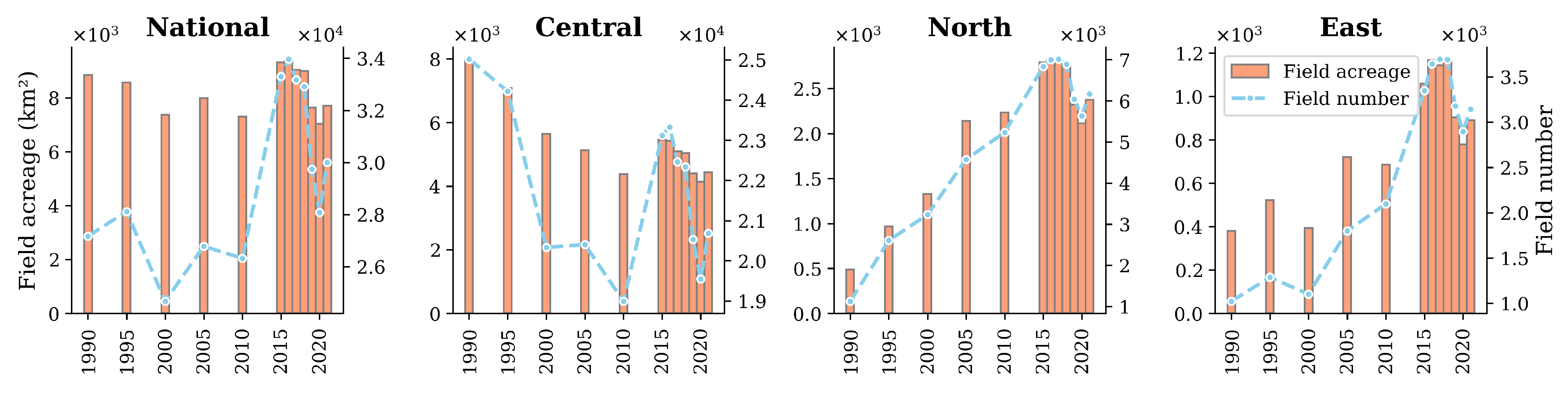
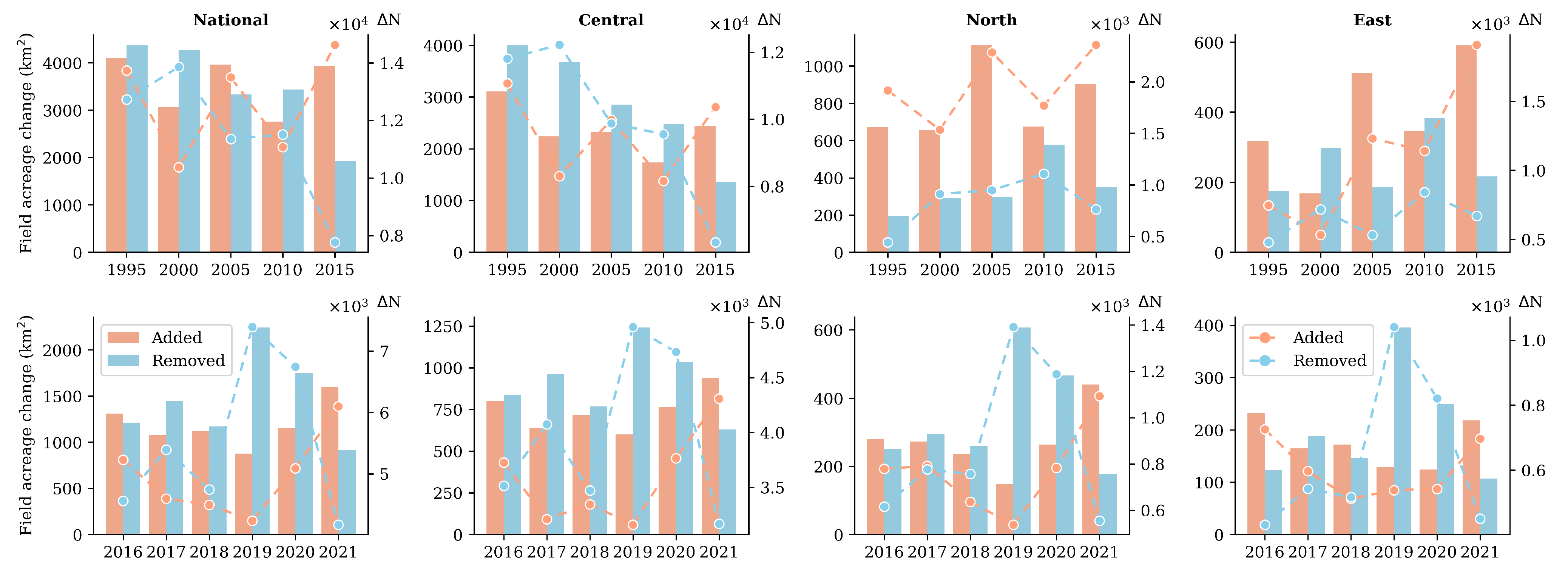
4.2.1. Multiple-Temporal Dynamics of Field Number and Acreage

The number and acreage of fields from 1990 to 2021 are shown in Figure 8. In 1990, more than 27,000 fields were detected covering a total area of 8841 km 2 . That period was followed by a decreasing trend until 2010, with an average extent of 8011 km 2 from 1990 to 2010. A major increase was observed from 2010 to 2015 with approximately 33,000 fields (representing 9310 km 2 ) being detected in 2015. The peak of the retrospective analysis was detected one year later in 2016, with 33,961 fields representing an area of 9408 km 2 . Since that time, the field acreage progressively decreased at an average rate of 6.9% (595 km 2 ) per year until 2020, with steep declines identified between 2018 and 2019, resulting in the field acreage reaching its lowest extent in 2020 (approximately 28,080 fields representing 7028 km 2 ). While 2021 saw a slight increase, the acreage for that year was still lower than the 1990 value. Overall, the largest expansion was observed from 2010 to 2015, when the number and acreage of the fields increased by 26.5 and 27.5%, respectively. On the other hand, the largest five-year reduction was observed from 2016 to 2020, when the number and acreage of fields decreased by 17.3 and 25.3%, respectively.
The central region (location shown in Figure 1) represented the hub of the agricultural development at the start of the study period, with 92% of the fields located within this region in 1990. That percentage decreased during the next two decades, although the central region still represented the majority with at least 68 and 56% in the number and acreage of the fields located therein in both 2017 and 2018. The trends in the northern and eastern regions were opposite to the central region for the first two decades (1990–2010), with those areas seeing an increasing number of fields and total acreage. The year 2016 represented a key point in the multi-decadal trends. As observed for the national estimates, both the north and east regions reached a maximum extent of fields. For the central region, 2016 also represented a local maximum extent of 5419 km 2 (23,330 fields) following the previous decreasing trend: although this was still much lower than the 1990 values, which comprised approximately 25,017 fields covering 7974 km 2 . More generally, the dynamics over the 6 years from 2015 to 2021 were similar for all the regions, witnessing a sharp decrease in agricultural development, with the largest change occurring from 2018 to 2019 as highlighted for the national estimates.
The hybrid machine learning framework for field delineation [47] offers additional insights related to the pattern of agricultural developments (Figure 9). For example, although the net change in the field acreage from 1990 to 1995 (−271 km 2 ) represented just a 3% decrease in fields, this was a consequence of 4098 km 2 of new fields and 4369 km 2 of older fields being removed. The newly created and removed field acreage accounted for 46.4 and 49.4% of the field acreage in 1990, which indicated that around 50% of the fields in Saudi Arabia were replaced from 1990 to 1995. With the denser record of Landsat imagery, that dynamic is shown yearly after 2015 (Figure 9). From these data, it can be observed that the numbers of newly created and removed fields were similar in 2016, 2017, and 2018, while significantly more fields were removed than created in 2019 and 2020.

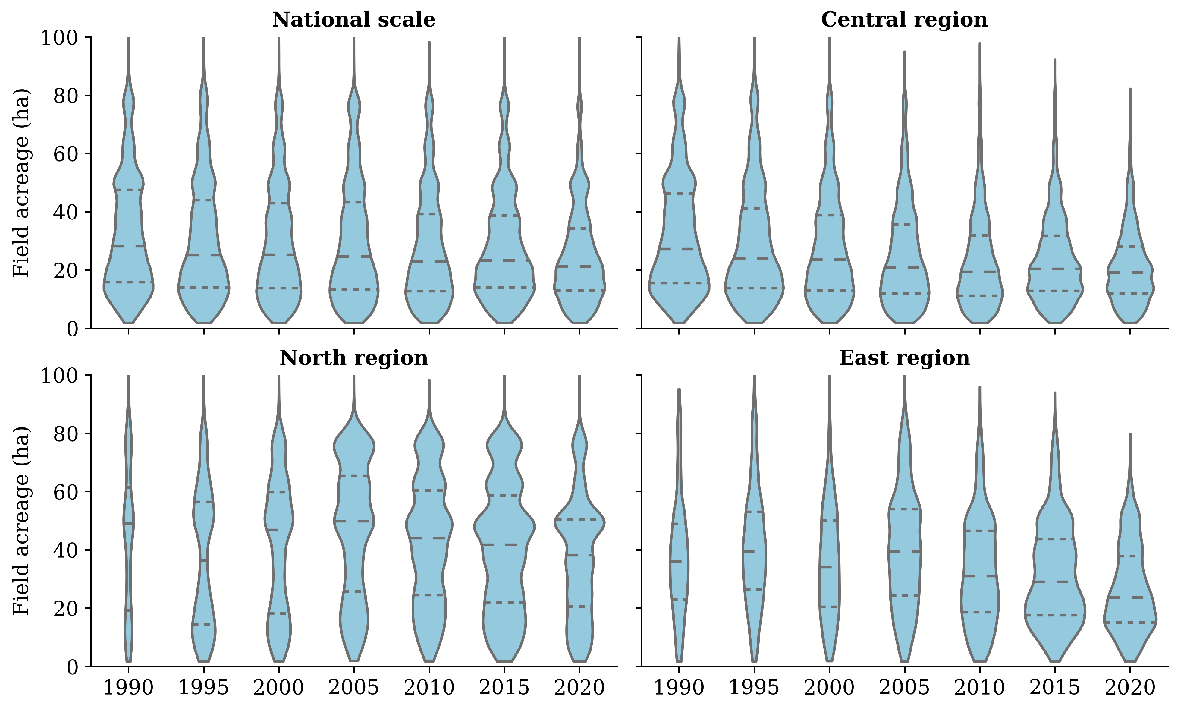
4.2.2. Multiple-Temporal Dynamics of Field Size Distribution

Figure 10 shows the distribution of the field acreage, with the width of the violins indicating the relative portion of the fields in each range of acreage. Nationally, the size of the fields in Saudi Arabia ranged from less than 10 ha to larger than 80 ha, with the most dominant size being 20 ha (representing a center-pivot irrigation system with an arm of 500 m in diameter). Regionally, there were some evident field size differences. Most of the fields in the north region were larger than the other two regions, e.g., around 50 ha (800 m in diameter), whereas most of the fields in the central and east regions had sizes of around 20 ha. The largest CPFs (e.g., 80 ha or more) were mainly observed in the north region, and were installed mostly between 2000 and 2005. In the central region, most of the large fields were phased out from 1990 to 2005.

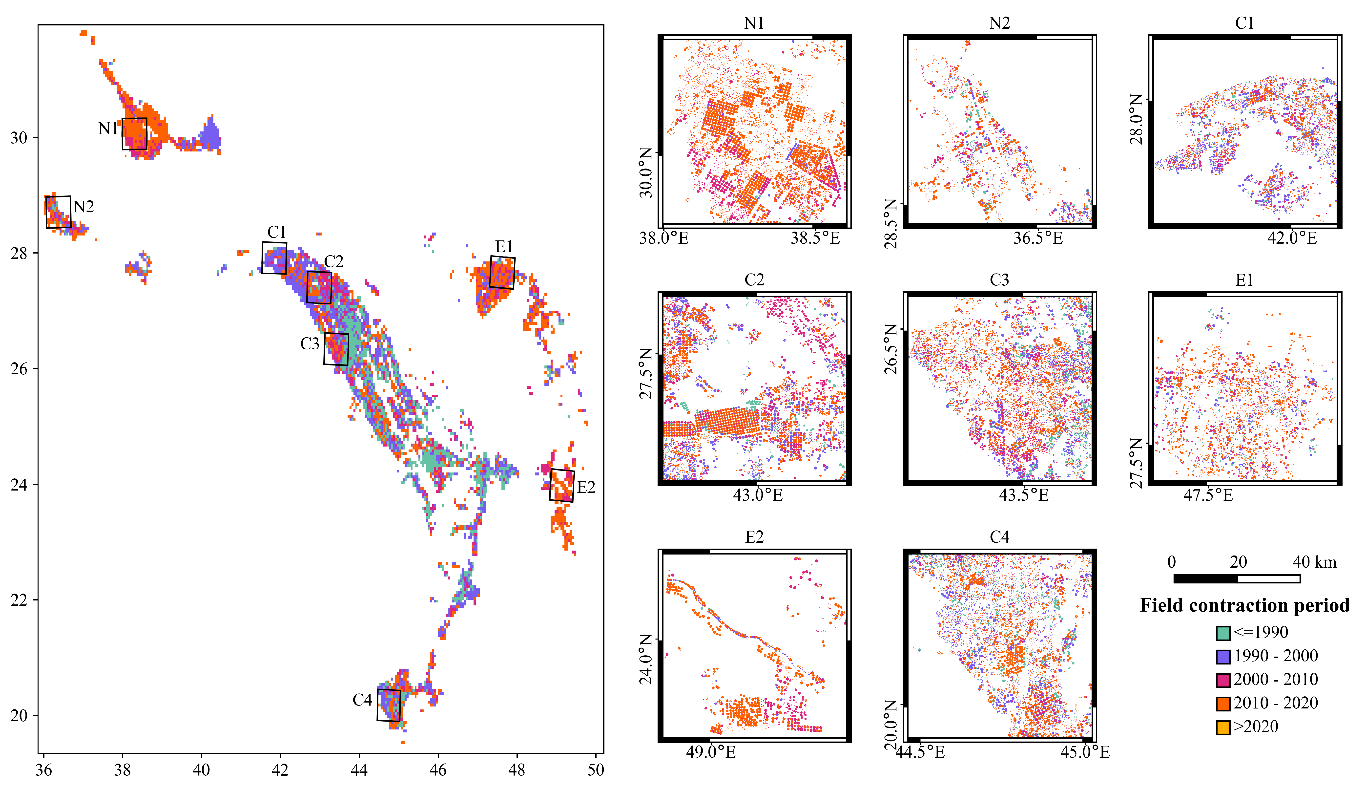
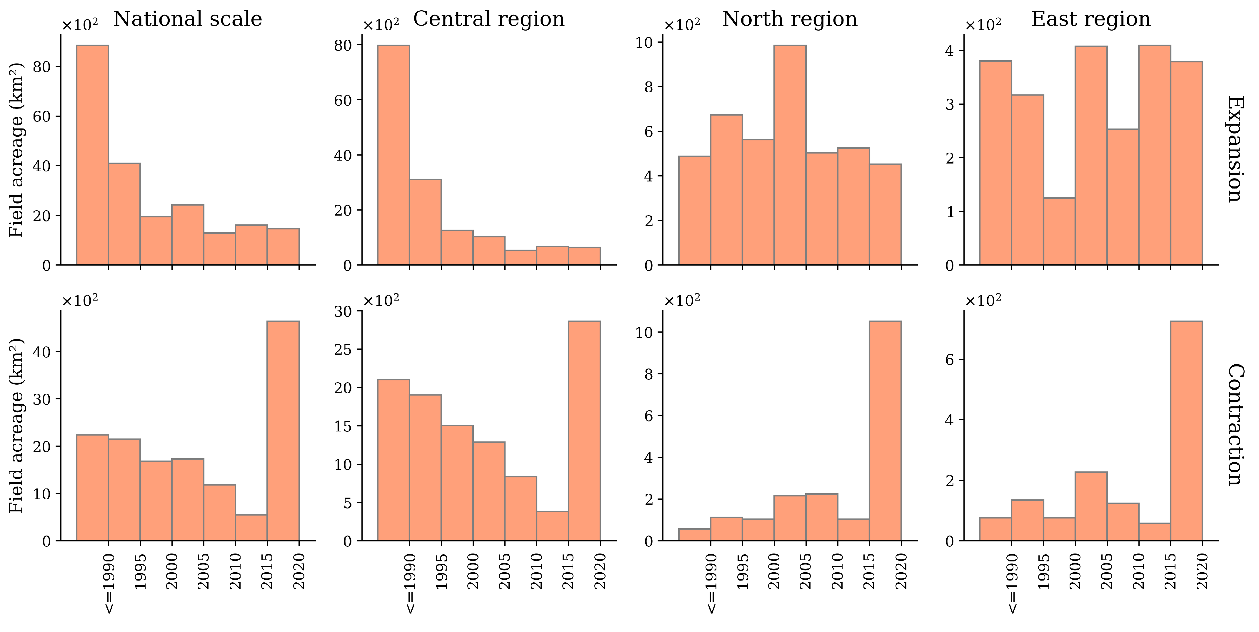
4.2.3. Field Expansion and Contraction Dynamics

The framework is also able to generate important spatiotemporal information such as field expansion and contraction maps (Figure 11 and Figure 12) and associated field acreage changes (Figure 13).These maps—generated at the pixel level—show the time at which a field was first detected and the year for which a field was last detected, respectively. Nationally, most of the fields were already installed by 1990 and were mostly within the central region (green color in Figure 11), with a total acreage of 8841 km 2 (Figure 13). A second expansive period was observed from 1991 to 1995, during which approximately 4095 km 2 of fields were added. In the north region-particularly in Al Jawf-the period from 2000 to 2010 also saw a significant expansion for field development, representing 1487 km 2 and accounting for 40% of the total expanding acreage after 1990 (Figure 11-N1 and Figure 13). Within the east region, the expansion of the fields occurred more sporadically over time (Figure 11-E1 and E2, and Figure 13). By contrast, most of the field phasing-out activities occurred after 2015 for all the regions (Figure 12 and Figure 13).
There were some interesting temporal trends related to field contraction. For example, around 2235 km 2 of of the fields that were detected in 1990 were no longer detected in all the ubsequent years (Figure 13), with the majority of such cases observed in the central region (green color in Figure 12). Such field contraction showed a decreasing trend with 338 km 2 of field acreage removed on average every five years until 2015 before peaking from 2016 to 2020, when around 4641 km 2 of the fields were abandoned at a national scale. A similar trend in the field contraction values was observed within the central region, which was not surprising, as it covers a significantly larger area (68 to 92% of the total field acreage) relative to the other regions. The field contraction trends were similar in the north and east regions, with relatively low contraction values prior to 2015, and large values after 2015, resulting in 1052 and 725 km 2 of eliminated fields between 2015 and 2020, respectively (Figure 13).

5. Discussion

Based on an application of a hybrid machine learning framework [47] that allowed for the accurate delineation of individual fields, the first multi-decadal assessment in terms of the number and acreage of center-pivot fields across Saudi Arabia was undertaken. In Section 5.1 we discuss how our results compare with the field acreage and accounting reported in the study of Johansen et al. [53], as well as against the Global Food Security-support Analysis Data (GFSAD) cropland extent map, one of the leading global agricultural mapping products. We also explore some of the implications and underlying drivers behind the development of these temporal patterns (Section 5.2), and identify some needed future work that may assist with the further interpretation and planning of the agricultural sector in Saudi Arabia and elsewhere (Section 5.3).

5.1. Intercomparison with Other Crop Mapping Products

The acreage and number of center-pivot fields presented here for the year 2015 were smaller than the national estimate reported in Johansen et al. [53] (11,555 km 2 against the 9310 km 2 estimated in this study). Other than methodological differences (an object-based image analysis versus a hybrid machine learning framework), the atmospheric method applied to Landsat-8 images presents as another likely reason for the discrepancy. The surface reflectance data used in this study were generated from the Land Surface Reflectance Code algorithm [70] (LSRC), while Johansen et al. [53] used the Second Simulation of the Satellite Signal in the Solar Spectrum (6SV) radiative transfer model [71]. In addition, the method proposed by Houborg and McCabe [72] was applied in Johansen et al. [53] to perform a regionally specific optimization that considered adjacency effects and non-spherical desert dust particles. As a result of the different atmosphere correction methods, the values of the annual maximum NDVI maps used as base maps in Johansen et al. [53] were higher than those herein. Moreover, Johansen et al. [53] used an NDVI threshold of 0.20 as opposed to the 0.25 threshold employed here, resulting in more pixels being counted when calculating the field acreage in Johansen et al. [53].
To verify the impact of the atmospheric correction, the framework was run using the annual maximum NDVI maps for three evaluation tiles (Figure 1) corrected by the 6SV method and with the regional optimization of the adjacency effect. A preliminary intercomparison between the resulting field delineation products was undertaken by comparing the distribution of the NDVI values for the pixels that were identified as fields using the 6SV correction but not with the LSRC correction (Figure A1). The distributions are skewed toward NDVI values lower than 0.3 within the LSRC-corrected base maps but show higher NDVI values within the 6SV-corrected maps. Because both delineation methods performed an initial filtering process based on a low NDVI threshold (0.25 for this study), this results in three pathways for a lower number of fields being detected in this study. First, fields with the majority of maximum annual NDVI values (using LSRC) of less than 0.25 were filtered at the start of the process in this study. Second, lower NDVI pixels along the boundaries of the fields were also not contributing to the total acreage. Finally, the shape of some fields was misclassified due to the presence of some low NDVI pixels, and thus these center-pivot fields were ultimately classified as non-center-pivot fields or eliminated as noise. Overall, while the LSRC-corrected maps resulted in fewer fields relative to Johansen et al. [53], they provide a significant advantage due to their availability on the Google Earth Engine, which served as an efficient tool for the multi-annual, large-scale dataset processing explored in this study.
An additional comparison (Figure A2) was made between our delineation result and that produced from the Global Food Security-support Analysis Data (GFSAD) cropland extent map (30 m spatial resolution) for the year 2015 [73]. The GFSAD is produced from multi-sensor remote sensing data using a random forest model [74]. The GFSAD map significantly overestimated (e.g., by approximately 56% in the Al Jawf region alone) the crop extent in Saudi Arabia relative to the present study, likely because the soil background pixels surrounded by fields were identified as crop pixels (green mask in Figure A2). In this case, our framework-delineated field map outperformed the GFSAD map in terms of accurately discriminating the agricultural extent from the soil background and providing individual field masks. However, the intent and purpose of the GFSAD is different in both scope and scale (i.e., it is a global product), and the complexity of our framework can also be considered a potential limitation for broad-scale application. Of course, the performance of our framework in regions other than Saudi Arabia remains to be explored, but it serves as a useful and needed exercise to compare local-to-regional-scale studies with available global datasets.

5.2. Socio-Political Drivers of Center-Pivot Field Dynamics

5.2.1. Agricultural Initialization Stage before 1990

Agricultural programs were initiated in Saudi Arabia with the First Development Plan of 1970–1975 [75]. Since then, development plans were released every five years until 2016, when the Saudi Vision 2030 [12] was proposed. Prior to 1990, agricultural development mainly occurred within the central region (Figure 8, Figure 11). Via the introduction of financial incentives such as a 50% discount on fertilizer and a guaranteed purchase price of 3.5 SAR/kg of wheat (The Third Development Plan 1980–1985) [76], the Kingdom achieved wheat self-sufficiency in the mid-1980s, and had even started to export wheat to other countries [77]. The Fifth Development Plan 1990–1995 [7] reported that the acreage of wheat fields reached 6020 km 2 in 1988, accounting for 53% of the total cropped area in that year. Given this, it can be inferred that most of the fields observed in the central region were likely to be growing wheat around 1990. However, as a consequence of the rapid agricultural development, the groundwater supplies suffered severe depletion. The Fourth Development Plan 1985–1990) [6] raised the issue of the impact of the increased agricultural output, especially wheat, on the rapid depletion of non-renewable water resources. As a solution, the objective of achieving a satisfactory rate of increase in farm output at minimum cost was proposed, and the incentive purchase price of wheat was reduced to 2 SAR/kg. Due to a lack of sufficient satellite data to undertake this analysis prior to 1990, our analysis did not capture the increase and potential decrease in fields prior to 1990. However, the decreasing trend of field acreage in the central region after 1990 (Figure 8) indeed reflected the expected outcome of the implemented initiatives.

5.2.2. Agricultural Contraction Stage from 1990 to 2010

An important turning point occurred during the Seventh and Eighth Development Plans [5,78], where self-sufficiency was no longer a strategic objective, but instead, the sustainable development of the agricultural sector became a focus. That had an immediate feedback on addressing the dramatic decline of non-renewable groundwater stock (by 60%) from 1979 to 2004 due to agriculture land expansion. By removing subsidies on the purchase price of wheat (Council of Ministers Resolution 264 of 2003), farmers were discouraged from growing wheat and encouraged to increase the diversity of crops. The wheat acreage subsequently decreased by 32.6% from 1994 to 1999, from 5820 to 3920 km 2 (The Seventh Development Plan 2000–2004) [78], which aligns with our results, when a sharp decrease of 1208 km 2 was observed in 2000 (Figure 8). However, our results only suggested a 14% reduction, possibly due to our research focus, which was limited to center-pivot fields, while the development plans considered all types of irrigated fields. Reports have shown that center-pivot systems were used to irrigate 67% of all fields in 2004 (Council of Ministers Resolution 217 of 2004). In addition, the increase in other crop types such as vegetables (e.g., tomatoes, melons, and dry onions) and fruit (e.g., dates and grapes) (increased from 2520 to 3180 km 2 from 1994 to 1999) could offset part of the acreage reduction by wheat because the government encouraged a diversified production of fruits and vegetables since the 1970s. Wheat production further decreased from 1999 to 2004, resulting in the wheat self-sufficiency ratio decreasing from 112.2 to 100% (The Eighth Development Plan 2005–2009) [5]. As such, it is reasonable to assume that most of the fields removed before 2010 (purple and green colors Figure 12) were mainly wheat fields. However, our results suggested an increase in the field number and acreage from 2000 to 2005. That might be a result of the policy initiative aimed at helping small farmers to make use of government support for center-pivot fields (Council of Ministers Resolution 217 of 2004), which resulted in more center-pivot fields being installed during 2004 to 2005. Thus, although the total irrigated acreage was expected to decrease, the acreage of center-pivot fields (the focus herein) increased from 2000 to 2005. Another decrease was observed from 2005 to 2010 (Figure 8), which might be a consequence of the five-year (2003–2008) suspension of the agricultural land distribution (The Eighth Development Plan 2005–2009) [5].

5.2.3. Agricultural Expansion Stage from 2010 to 2016

A policy was also initiated in the Eighth Development Plan to provide information and conduct research to assess the most competitive agricultural activities. No clear replacement crops were presented to the farmers when phasing out wheat. Without specific guidance, farmers started to grow alfalfa and other fodder crops to support a growing dairy industry [9]. Wheat’s share of the total crop acreage dropped from 29.7 to 14.4% from 2010 to 2015, while the share of fodder crops increased from 25.0 to 59.1% for the same period [79,80,81,82,83,84]. As a result, alfalfa became one of the most planted field crops from 2010, which is reflected in the significant increase in the field acreage observed in 2015 (Figure 8 and Figure 9). As such, the newly created fields from 2005 to 2015 in Figure 11 were likely alfalfa fields and mainly distributed in the north and east regions of the country. Unfortunately, alfalfa tends to be irrigated all year round and can consume up to five times the amount of water required by wheat. Thus, unregulated crop replacement did not achieve the goal of saving water. Given the observed impact of growing fodder crops on groundwater resources, a policy of banning the cultivation of green fodder was introduced in 2015 [85]. Furthermore, the non-renewable groundwater consumption in the agricultural sector was expected to decrease by 47% from 17 billion m 3 in 2016 to 9 billion m 3 in 2020 as proposed by the National Water Strategy 2030 [10], which resulted in a consistent decrease in fields after 2016 (Figure 8 and Figure 9). As such, the eliminated fields from 2016 to 2020 observed in Figure 12 were most likely alfalfa fields. On the other hand, a clear policy was initiated to promote the cultivation of fruit trees best suited to the Kingdom’s environment, such as olive trees in Al Jawf, tropical fruits in Jazan, and citruses in Najran (The Ninth Development Plan 2010–2014) [11]. That was in agreement with the results in Li et al. [47], which showed a significant increase in olive orchards in the Al Jawf region since 2010. However, it remains a question whether growing olives can save more water than wheat or alfalfa production given the high water footprint of olive (3015 m 3 / ton) compared to fodder crops (1887 m 3 / ton) and wheat (1868 m 3 / ton) [86,87].

5.2.4. Agricultural Contraction Stage since 2016

The annual analysis of the recent past seven years (2015–2021) indicated a clear overall decrease in the number of center-pivot fields from the peak levels in 2016 in subsequent years, particularly between 2018 and 2019. However, the change from 2020 to 2021 (Figure 8 and Figure 9), as well as a preliminary analysis of the current year (2022) which is still ongoing, indicate a more recent uptick in fields under active production, in contrast to the previously observed declines. A plausible explanation for these trends is in response to global influences, including both the pandemic and the more recent conflict in Ukraine, which have seen disruptions in international supply, logistics, and trade. A future analysis using this framework will be able to quantify the degree, and speed, at which the local agricultural sector was able to respond to these global perturbations, providing insights into the resilience and elasticity of the Saudi Arabian food system.

5.3. Future Work

The development of a scalable framework for field delineation allows for the identification and description of agricultural dynamics at the national scale. The changing trends and variations identified herein provide both a quantification of the number and acreage of the fields as well as the geographical distribution of these temporal dynamics. One obvious advantage of such an analysis is that it provides a tool for decision-makers to determine the relative impact of agricultural management policy initiatives, and whether they have the intended outcomes. As a further application, the produced field maps may also be used for compliance purposes to assess if farmers are in fact adhering to implemented policy initiatives for crop production and a reduction in irrigation and water use [88].
While the image processing framework achieved high field delineation accuracies across the Kingdom, there were some limitations when (1) fields were overlapping, especially if the overlapping fields had different sizes and/or shapes, and (2) fields were small or had low maximum annual NDVI values. The overlapping fields were the main cause of error in this framework, i.e., fields being under-segmented. One of the most straightforward solutions could be to use satellite imagery with a higher spatial resolution, such as Sentinel-2 (10 m bands) [89] and PlanetScope (~3 m bands) [90], albeit coming with a higher computational cost. According to our analysis, one of the reasons for under-segmentation was that the CNN approach misclassified the field objects consisting of multiple fields into one field object. The current CNN model in the framework was trained using data from the north region in 2018, where the fields were well distributed and with a relatively uniform size. Field objects consisting of large fields overlapping with small fields did not exist in this training sample. A higher CNN classification accuracy might be achieved by re-training the model using more representative data collected from various locations and times [91], which would require the manual classification of smaller fields and combinations of overlapping fields. Gap-filling methods to reduce the stripes in the Landsat-7 data are worth exploring to reduce the over-segmentation errors [92]. Another challenge was the discrimination of the agricultural pixels from the bare soil, which was done simply by eliminating pixels with an annual maximum NDVI value of less than 0.25. However, this threshold filtration might not work in other non-desert environments where natural vegetation is present. Using indices such as the Soil Adjustment Vegetation Index, which considers the soil spectra as the framework input, is worth exploring [49,93]. Future work should also explore the use of other vegetation indices, such as the Enhanced Vegetation Index, which is less impacted by the atmospherical condition than the NDVI, to assess the impact and potential improvement in mapping accuracies of center-pivot fields [94]. Machine learning techniques (e.g., random forest) are also considered to discriminate between bare soil, natural vegetation, and crops in the initial stage of the framework [95], opening many avenues for ongoing research and investigation.

6. Conclusions

A three-decades-long retrospective analysis of center-pivot-driven agricultural development was performed across the main agricultural regions of Saudi Arabia. A hybrid machine learning framework implementing DBSCAN, CNN classification, and spectral clustering in a sequential manner was applied to delineate center-pivot fields utilizing annual maximum NDVI maps obtained from Landsat imagery (Landsat 4/5/7/8) since 1990. The framework achieved high field delineation accuracies when applied to different regions (i.e., Landsat tiles 165/41, 166/46, and 168/42 in path/row) and periods (i.e., 2000, 2010, and 2015), resulting in 83.7–94.8% and 90.2–97.9% producer’s and user’s accuracies at the object level, respectively. The extent of the individual center-pivot fields was delineated accurately, with the median value of the over-segmentation, under-segmentation, and intersection over union error being 2.1, 0.9, and 5%, respectively. The coefficient of determination ( R 2 ) for the acreage between the framework-delineated fields and ground-truth fields was higher than 0.97.
The results presented herein provide new insights into the development of the agricultural sector in Saudi Arabia on a national scale. For the first time, the number and acreage of center-pivot fields, the distribution of field sizes, and the expansion and contraction dynamics for the most recent thirty years were characterized. The major trends and variations in the field dynamics identified within this study broadly reflected the effects of successive policy initiatives on agriculture development. From 1970 to1990, the policy initiatives in Saudi Arabia stimulated an increase in agricultural production and the number of center-pivot fields. The gradual decrease observed between 1990 and 2010 was the outcome of the policy initiatives implemented to phase out wheat, which had exceeded the self-sufficiency level of the Kingdom by the mid-1980s. Increases in the cultivated area seen from 2010 to 2015 were a consequence of wheat fields being replaced by fodder crops, with the latter being phased out since 2016 to save water. However, the framework presented some limitations when dealing with overlapping fields, so additional exploration will need to focus on reducing the under-segmentation errors caused by the overlap. Such framework developments might include an assessment of additional vegetation indices as input, the collection of more training samples from different regions and periods, and the implementation of machine learning techniques to discriminate bare soil from crops. Through this study, the capability of a regionally focused machine learning framework applied at the national scale was demonstrated. Apart from delivering actionable information for decision-makers on long-term agricultural patterns and dynamics, the field masks and the subsequent agro-informatics retrieved from this study will prove useful as baseline information for future food- and water-security-related studies.

Author Contributions

T.L.: Conceptualization, Methodology, Coding, Validation, Visualization, Writing—original draft, Writing—review & editing. O.M.L.V.: Visualization, Writing—review & editing. K.J.: Writing— review & editing. M.F.M.: Conceptualization, Supervision, Writing—review & editing. All authors have read and agreed to the published version of the manuscript.

Funding

Research reported in this publication was supported by the King Abdullah University of Science and Technology (KAUST).

Data Availability Statement

Not applicable.

Conflicts of Interest

The authors declare no conflict of interest.

Appendix A

Figure A1. The NDVI distributions of pixels detected as pixels forming a center-pivot field using 6SV-corrected maps, but not detected using LSRC-corrected maps. The grey line indicates NDVI = 0.25.
Remotesensing 15 00731 g0a1
Figure A2. An example of a maximum annual NDVI map associated with the Global Food Security-support Analysis Data (GFSAD) cropland extent map (30 m spatial resolution) and the framework delineation result.
Remotesensing 15 00731 g0a2

References

  1. Wada, Y.; Wisser, D.; Eisner, S.; Flörke, M.; Gerten, D.; Haddeland, I.; Hanasaki, N.; Masaki, Y.; Portmann, F.T.; Stacke, T.; et al. Multimodel projections and uncertainties of irrigation water demand under climate change. Geophys. Res. Lett. 2013, 40, 4626–4632. [Google Scholar] [CrossRef] [Green Version]
  2. López Valencia, O.M.; Johansen, K.; Aragón Solorio, B.J.L.; Li, T.; Houborg, R.; Malbeteau, Y.; AlMashharawi, S.; Altaf, M.U.; Fallatah, E.M.; Dasari, H.P.; et al. Mapping groundwater abstractions from irrigated agriculture: Big data, inverse modeling, and a satellite–model fusion approach. Hydrol. Earth Syst. Sci. 2020, 24, 5251–5277. [Google Scholar] [CrossRef]
  3. GebreEgziabher, M.; Jasechko, S.; Perrone, D. Widespread and increased drilling of wells into fossil aquifers in the USA. Nat. Commun. 2022, 13, 2129. [Google Scholar] [CrossRef]
  4. Elhadj, E. Camels don’t fly, deserts don’t bloom: An assessment of Saudi Arabia’s experiment in desert agriculture. Occasional Paper. 2004, 49. [Google Scholar]
  5. Ministry of Economy and Planning. Eighth Development Plan 2005–2009; Ministry of Economy and Planning: Riyadh, Saudi Arabia, 2005.
  6. Ministry of Economy and Planning. Fourth Development Plan 1985–1990; Ministry of Economy and Planning: Riyadh, Saudi Arabia, 1985.
  7. Ministry of Economy and Planning. Fifth Development Plan 1990–1995; Ministry of Economy and Planning: Riyadh, Saudi Arabia, 1990.
  8. Ministry of Economy and Planning. Sixth Development Plan 1995–2000; Ministry of Economy and Planning: Riyadh, Saudi Arabia, 1995.
  9. Kim, A.; van der Beek, H. A holistic assessment of the water-for-agriculture dilemma in the Kingdom of Saudi Arabia. CIRS Occas. Pap. 2018. [Google Scholar]
  10. MEWA. National Water Strategy. Available online: https://www.mewa.gov.sa/en/Ministry/Agencies/TheWaterAgency/Topics/Pages/Strategy.aspx (accessed on 3 October 2022).
  11. Ministry of Economy and Planning. Ninth Development Plan 2010–2014; Ministry of Economy and Planning: Riyadh, Saudi Arabia, 2010.
  12. Kingdom of Saudi Arabia. Vision 2030. Available online: https://www.vision2030.gov.sa/ (accessed on 3 October 2022).
  13. FAO. Country Profile—Saudi Arabia; FAO: Rome, Italy, 2008. [Google Scholar]
  14. World Bank. A Water Sector Assessment Report on Countries of the Cooperation Council of the Arab State of the Gulf; Report No. 32539-MNA; World Bank: Washington, DC, USA, 2005. [Google Scholar]
  15. Aragon, B.; Houborg, R.; Tu, K.; Fisher, J.B.; McCabe, M. CubeSats Enable High Spatiotemporal Retrievals of Crop-Water Use for Precision Agriculture. Remote Sens. 2018, 10, 1867. [Google Scholar] [CrossRef] [Green Version]
  16. De Albuquerque, A.O.; de Carvalho, O.L.F.; e Silva, C.R.; Luiz, A.S.; Pablo, P.; Gomes, R.A.T.; Guimarães, R.F.; de Carvalho Júnior, O.A. Dealing With Clouds and Seasonal Changes for Center Pivot Irrigation Systems Detection Using Instance Segmentation in Sentinel-2 Time Series. IEEE J. Sel. Top. Appl. Earth Obs. Remote Sens. 2021, 14, 8447–8457. [Google Scholar] [CrossRef]
  17. Carlson, M.P. The Nebraska Center-Pivot Inventory: An example of operational satellite remote sensing on a long-term basis. Photogramm. Eng. Remote Sens. 1989, 55, 587–590. [Google Scholar]
  18. Giri, C.; Pengra, B.; Long, J.; Loveland, T.R. Next generation of global land cover characterization, mapping, and monitoring. Int. J. Appl. Earth Obs. Geoinf. 2013, 25, 30–37. [Google Scholar] [CrossRef]
  19. Tchuenté, A.T.K.; Roujean, J.L.; De Jong, S.M. Comparison and relative quality assessment of the GLC2000, GLOBCOVER, MODIS and ECOCLIMAP land cover data sets at the African continental scale. Int. J. Appl. Earth Obs. Geoinf. 2011, 13, 207–219. [Google Scholar] [CrossRef]
  20. Ferreira, E.; Toledo, J.H.d.; Dantas, A.A.; Pereira, R.M. Cadastral maps of irrigated areas by center pivots in the State of Minas Gerais, using CBERS-2B/CCD satellite imaging. Eng. Agríc. 2011, 31, 771–780. [Google Scholar] [CrossRef] [Green Version]
  21. Litts, T.; Russell, H.; Thomas, A.; Welch, R. Mapping Irrigated Lands in the ACF River Basin; Georgia Institute of Technology: Atlanta, GA, USA, 2001. [Google Scholar]
  22. Seth, N. Analyzing the Increase in Center Pivot Irrigation Systems in Custer County, Nebraska USA from 2003 to 2010. Pap. Resour. Anal. 2015, 17, 15. [Google Scholar]
  23. Graesser, J.; Ramankutty, N. Detection of cropland field parcels from Landsat imagery. Remote Sens. Environ. 2017, 201, 165–180. [Google Scholar] [CrossRef] [Green Version]
  24. Watkins, B.; Van Niekerk, A. A comparison of object-based image analysis approaches for field boundary delineation using multi-temporal Sentinel-2 imagery. Comput. Electron. Agric. 2019, 158, 294–302. [Google Scholar] [CrossRef]
  25. Yan, L.; Roy, D.P. Automated crop field extraction from multi-temporal Web Enabled Landsat Data. Remote Sens. Environ. 2014, 144, 42–64. [Google Scholar] [CrossRef] [Green Version]
  26. Yan, L.; Roy, D.P. Conterminous United States crop field size quantification from multi-temporal Landsat data. Remote Sens. Environ. 2016, 172, 67–86. [Google Scholar] [CrossRef] [Green Version]
  27. Canny, J. A computational approach to edge detection. IEEE Trans. Pattern Anal. Mach. Intell. 1986, PAMI-8, 679–698. [Google Scholar] [CrossRef]
  28. Baatz, M. Multi Resolution Segmentation: An Optimum Approach for High Quality Multi Scale Image Segmentation; Beutrage zum AGIT-Symposium: Salzburg, Austria, 2000; pp. 12–23. [Google Scholar]
  29. Bleau, A.; Leon, L.J. Watershed-based segmentation and region merging. Comput. Vis. Image Underst. 2000, 77, 317–370. [Google Scholar] [CrossRef]
  30. Koc-San, D.; Selim, S.; Aslan, N.; San, B.T. Automatic citrus tree extraction from UAV images and digital surface models using circular Hough transform. Comput. Electron. Agric. 2018, 150, 289–301. [Google Scholar] [CrossRef]
  31. Rodrigues, M.; Körting, T.; de Queiroz, G.; Sales, C.; da Silva, L. Detecting center pivots in Matopiba using Hough transform and web time series service. In Proceedings of the 2020 IEEE Latin American GRSS & ISPRS Remote Sensing Conference (LAGIRS), Santiago, Chile, 22–26 March 2020; pp. 189–194. [Google Scholar]
  32. Garcia-Pedrero, A.; Gonzalo-Martin, C.; Lillo-Saavedra, M. A machine learning approach for agricultural parcel delineation through agglomerative segmentation. Int. J. Remote Sens. 2017, 38, 1809–1819. [Google Scholar] [CrossRef] [Green Version]
  33. Lebourgeois, V.; Dupuy, S.; Vintrou, E.; Ameline, M.; Butler, S.; Bégué, A. A combined random forest and OBIA classification scheme for mapping smallholder agriculture at different nomenclature levels using multisource data (simulated Sentinel-2 time series, VHRS and DEM). Remote Sens. 2017, 9, 259. [Google Scholar] [CrossRef] [Green Version]
  34. Long, J.; Li, M.; Wang, X.; Stein, A. Delineation of agricultural fields using multi-task BsiNet from high-resolution satellite images. Int. J. Appl. Earth Obs. Geoinf. 2022, 112, 102871. [Google Scholar] [CrossRef]
  35. LeCun, Y.; Boser, B.; Denker, J.S.; Henderson, D.; Howard, R.E.; Hubbard, W.; Jackel, L.D. Backpropagation applied to handwritten zip code recognition. Neural Comput. 1989, 1, 541–551. [Google Scholar] [CrossRef]
  36. Zhang, C.; Yue, P.; Di, L.; Wu, Z. Automatic identification of center pivot irrigation systems from landsat images using convolutional neural networks. Agriculture 2018, 8, 147. [Google Scholar] [CrossRef] [Green Version]
  37. Krizhevsky, A.; Sutskever, I.; Hinton, G.E. Imagenet classification with deep convolutional neural networks. Commun. ACM 2017, 60, 84–90. [Google Scholar] [CrossRef] [Green Version]
  38. LeCun, Y.; Bengio, Y. Convolutional networks for images, speech, and time series. Handb. Brain Theory Neural Netw. 1995, 3361, 1995. [Google Scholar]
  39. Simonyan, K.; Zisserman, A. Very deep convolutional networks for large-scale image recognition. arXiv 2014, arXiv:1409.1556. [Google Scholar]
  40. De Albuquerque, A.O.; de Carvalho Júnior, O.A.; Carvalho, O.L.F.d.; de Bem, P.P.; Ferreira, P.H.G.; de Moura, R.d.S.; Silva, C.R.; Trancoso Gomes, R.A.; Fontes Guimarães, R. Deep semantic segmentation of center pivot irrigation systems from remotely sensed data. Remote Sens. 2020, 12, 2159. [Google Scholar] [CrossRef]
  41. Graf, L.; Bach, H.; Tiede, D. Semantic Segmentation of Sentinel-2 Imagery for Mapping Irrigation Center Pivots. Remote Sens. 2020, 12, 3937. [Google Scholar] [CrossRef]
  42. Saraiva, M.; Protas, E.; Salgado, M.; Souza, C., Jr. Automatic mapping of center pivot irrigation systems from satellite images using deep learning. Remote Sens. 2020, 12, 558. [Google Scholar] [CrossRef] [Green Version]
  43. De Albuquerque, A.O.; de Carvalho, O.L.F.; e Silva, C.R.; de Bem, P.P.; Gomes, R.A.T.; Borges, D.L.; Guimarães, R.F.; Pimentel, C.M.M.; de Carvalho Júnior, O.A. Instance segmentation of center pivot irrigation systems using multi-temporal SENTINEL-1 SAR images. Remote Sens. Appl. Soc. Environ. 2021, 23, 100537. [Google Scholar] [CrossRef]
  44. Mekhalfi, M.L.; Nicolò, C.; Bazi, Y.; Al Rahhal, M.M.; Al Maghayreh, E. Detecting Crop Circles in Google Earth Images with Mask R-CNN and YOLOv3. Appl. Sci. 2021, 11, 2238. [Google Scholar] [CrossRef]
  45. Tang, J.; Arvor, D.; Corpetti, T.; Tang, P. Mapping Center Pivot Irrigation Systems in the Southern Amazon from Sentinel-2 Images. Water 2021, 13, 298. [Google Scholar] [CrossRef]
  46. Waldner, F.; Diakogiannis, F.I. Deep learning on edge: Extracting field boundaries from satellite images with a convolutional neural network. Remote Sens. Environ. 2020, 245, 111741. [Google Scholar] [CrossRef]
  47. Li, T.; Johansen, K.; McCabe, M.F. A machine learning approach for identifying and delineating agricultural fields and their multi-temporal dynamics using three decades of Landsat data. ISPRS J. Photogramm. Remote Sens. 2022, 186, 83–101. [Google Scholar] [CrossRef]
  48. Aghighi, H.; Azadbakht, M.; Ashourloo, D.; Shahrabi, H.S.; Radiom, S. Machine learning regression techniques for the silage maize yield prediction using time-series images of Landsat 8 OLI. IEEE J. Sel. Top. Appl. Earth Obs. Remote Sens. 2018, 11, 4563–4577. [Google Scholar] [CrossRef]
  49. Belgiu, M.; Csillik, O. Sentinel-2 cropland mapping using pixel-based and object-based time-weighted dynamic time warping analysis. Remote Sens. Environ. 2018, 204, 509–523. [Google Scholar] [CrossRef]
  50. Yan, D.; Zhang, X.; Nagai, S.; Yu, Y.; Akitsu, T.; Nasahara, K.N.; Ide, R.; Maeda, T. Evaluating land surface phenology from the Advanced Himawari Imager using observations from MODIS and the Phenological Eyes Network. Int. J. Appl. Earth Obs. Geoinf. 2019, 79, 71–83. [Google Scholar] [CrossRef]
  51. Senay, G.B.; Schauer, M.; Friedrichs, M.; Velpuri, N.M.; Singh, R.K. Satellite-based water use dynamics using historical Landsat data (1984–2014) in the southwestern United States. Remote Sens. Environ. 2017, 202, 98–112. [Google Scholar] [CrossRef]
  52. El Kenawy, A.M.; McCabe, M.F. A multi-decadal assessment of the performance of gauge-and model-based rainfall products over Saudi Arabia: Climatology, anomalies and trends. Int. J. Climatol. 2016, 36, 656–674. [Google Scholar] [CrossRef] [Green Version]
  53. Johansen, K.; Lopez, O.; Tu, Y.H.; Li, T.; McCabe, M.F. Center pivot field delineation and mapping: A satellite-driven object-based image analysis approach for national scale accounting. ISPRS J. Photogramm. Remote Sens. 2021, 175, 1–19. [Google Scholar] [CrossRef]
  54. General Authority for Statistics. The Statistical Yearbook 2019; General Authority for Statistics: Riyadh, Saudi Arabia, 2019. [Google Scholar]
  55. Gorelick, N.; Hancher, M.; Dixon, M.; Ilyushchenko, S.; Thau, D.; Moore, R. Google Earth Engine: Planetary-scale geospatial analysis for everyone. Remote Sens. Environ. 2017, 202, 18–27. [Google Scholar] [CrossRef]
  56. Scaramuzza, P.; Barsi, J. Landsat 7 scan line corrector-off gap-filled product development. In Proceedings of the Pecora 16 Global Priorities in Land Remote Sensing, Sioux Falls, SD, USA, 23–27 October 2005; Volume 16, pp. 23–27. [Google Scholar]
  57. Chen, J.; Zhu, X.; Vogelmann, J.E.; Gao, F.; Jin, S. A simple and effective method for filling gaps in Landsat ETM+ SLC-off images. Remote Sens. Environ. 2011, 115, 1053–1064. [Google Scholar] [CrossRef]
  58. Ester, M.; Kriegel, H.P.; Sander, J.; Xu, X. A density-based algorithm for discovering clusters in large spatial databases with noise. In Proceedings of the KDD-96: Proceedings, Portland, OR, USA, 2–4 August 1996; Volume 96, pp. 226–231. [Google Scholar]
  59. Von Luxburg, U. A tutorial on spectral clustering. Stat. Comput. 2007, 17, 395–416. [Google Scholar] [CrossRef]
  60. Tan, P.N.; Steinbach, M.; Kumar, V. Cluster analysis: Basic concepts and algorithms. Introd. Data Min. 2006, 8, 526–533. [Google Scholar]
  61. Ferrara, R.; Virdis, S.G.; Ventura, A.; Ghisu, T.; Duce, P.; Pellizzaro, G. An automated approach for wood-leaf separation from terrestrial LIDAR point clouds using the density based clustering algorithm DBSCAN. Agric. For. Meteorol. 2018, 262, 434–444. [Google Scholar] [CrossRef]
  62. Tao, S.; Wu, F.; Guo, Q.; Wang, Y.; Li, W.; Xue, B.; Hu, X.; Li, P.; Tian, D.; Li, C. Segmenting tree crowns from terrestrial and mobile LiDAR data by exploring ecological theories. ISPRS J. Photogramm. Remote Sens. 2015, 110, 66–76. [Google Scholar] [CrossRef] [Green Version]
  63. Hopfield, J.J. Neural networks and physical systems with emergent collective computational abilities. Proc. Natl. Acad. Sci. USA 1982, 79, 2554–2558. [Google Scholar] [CrossRef] [Green Version]
  64. Schmidhuber, J. Deep learning in neural networks: An overview. Neural Netw. 2015, 61, 85–117. [Google Scholar] [CrossRef] [Green Version]
  65. Shi, J.; Malik, J. Normalized cuts and image segmentation. Dep. Pap. (CIS) 2000, 22, 107. [Google Scholar]
  66. Tung, F.; Wong, A.; Clausi, D.A. Enabling scalable spectral clustering for image segmentation. Pattern Recognit. 2010, 43, 4069–4076. [Google Scholar] [CrossRef]
  67. Dhillon, I.S.; Guan, Y.; Kulis, B. Kernel k-means: Spectral clustering and normalized cuts. In Proceedings of the Tenth ACM SIGKDD International Conference on Knowledge Discovery and Data Mining, Seattle, WA, USA, 22–25 August 2004; pp. 551–556. [Google Scholar]
  68. Ng, A.; Jordan, M.; Weiss, Y. On spectral clustering: Analysis and an algorithm. In Proceedings of the Advances in Neural Information Processing Systems (NIPS), Vancouver, BC, Canada, 3–8 December 2001. [Google Scholar]
  69. Caliński, T.; Harabasz, J. A dendrite method for cluster analysis. Commun.-Stat.-Theory Methods 1974, 3, 1–27. [Google Scholar] [CrossRef]
  70. Vermote, E.; Justice, C.; Claverie, M.; Franch, B. Preliminary analysis of the performance of the Landsat 8/OLI land surface reflectance product. Remote Sens. Environ. 2016, 185, 46–56. [Google Scholar] [CrossRef]
  71. Kotchenova, S.Y.; Vermote, E.F.; Matarrese, R.; Klemm, F.J., Jr. Validation of a vector version of the 6S radiative transfer code for atmospheric correction of satellite data. Part I: Path radiance. Appl. Opt. 2006, 45, 6762–6774. [Google Scholar] [CrossRef] [Green Version]
  72. Houborg, R.; McCabe, M.F. Impacts of dust aerosol and adjacency effects on the accuracy of Landsat 8 and RapidEye surface reflectances. Remote Sens. Environ. 2017, 194, 127–145. [Google Scholar] [CrossRef]
  73. Phalke, A.; Özdoğan, M.; Thenkabail, P.; Congalton, R.; Yadav, K.; Massey, R.; Teluguntla, P.; Poehnelt, J.; Smith, C. NASA Making Earth System Data Records for Use in Research Environments (MEaSUREs) Global Food Security-support Analysis Data (GFSAD) Cropland Extent 2015 Europe, Central Asia, Russia, Middle East 30 m V001 [Dataset] NASA EOSDIS Land Processes DAAC. Available online: https://www.researchgate.net/publication/331906826_NASA_Making_Earth_System_Data_Records_for_Use_in_Research_Environments_MEaSUREs_Global_Food_Security-support_Analysis_Data_GFSAD_Cropland_Extent_2015_Europe_Central_Asia_Russia_Middle_East_30_m_V001 (accessed on 12 October 2022).
  74. Phalke, A.R.; Özdoğan, M.; Thenkabail, P.S.; Erickson, T.; Gorelick, N.; Yadav, K.; Congalton, R.G. Mapping croplands of Europe, middle east, russia, and central asia using landsat, random forest, and google earth engine. ISPRS J. Photogramm. Remote Sens. 2020, 167, 104–122. [Google Scholar] [CrossRef]
  75. Ministry of Economy and Planning. First Development Plan 1970–1975; Ministry of Economy and Planning: Riyadh, Saudi Arabia, 1970.
  76. Ministry of Economy and Planning. Third Development Plan 1980–1985; Ministry of Economy and Planning: Riyadh, Saudi Arabia, 1980.
  77. Al-Subaiee, S.S.; Yoder, E.P.; Thomson, J.S. Extension agents’ perceptions of sustainable agriculture in the Riyadh Region of Saudi Arabia. J. Int. Agric. Ext. Educ. 2005, 12, 5–14. [Google Scholar] [CrossRef]
  78. Ministry of Planning. Seventh Development Plan 2000–2004; Ministry of Economy and Planning: Riyadh, Saudi Arabia, 2000.
  79. General Authority for Statistics. The Statistical Yearbook 2011; General Authority for Statistics: Riyadh, Saudi Arabia, 2011.
  80. General Authority for Statistics. The Statistical Yearbook 2012; General Authority for Statistics: Riyadh, Saudi Arabia, 2012.
  81. General Authority for Statistics. The Statistical Yearbook 2013; General Authority for Statistics: Riyadh, Saudi Arabia, 2013.
  82. General Authority for Statistics. The Statistical Yearbook 2014; General Authority for Statistics: Riyadh, Saudi Arabia, 2014.
  83. General Authority for Statistics. The Statistical Yearbook 2015; General Authority for Statistics: Riyadh, Saudi Arabia, 2015.
  84. General Authority for Statistics. The Statistical Yearbook 2016; General Authority for Statistics: Riyadh, Saudi Arabia, 2016.
  85. Alamri, Y.; Reed, M.R. Estimating virtual water trade in crops for saudi arabia. Am. J. Water Resour. 2019, 7, 16–22. [Google Scholar]
  86. Multsch, S.; Alrumaikhani, Y.; Alharbi, O.; Breuer, L. Internal water footprint assessment of Saudi Arabia using the water footprint assessment framework (WAF). In Proceedings of the 19th International Congress on Modelling and Simulation, Perth, Australia, 12–16 December 2011. [Google Scholar]
  87. Mekonnen, M.M.; Hoekstra, A.Y. The green, blue and grey water footprint of crops and derived crop products. Hydrol. Earth Syst. Sci. 2011, 15, 1577–1600. [Google Scholar] [CrossRef] [Green Version]
  88. McCabe, M.; Aragon, B.; Houborg, R.; Mascaro, J. CubeSats in Hydrology: Ultrahigh-Resolution Insights Into Vegetation Dynamics and Terrestrial Evaporation. Water Resour. Res. 2017, 53, 10017–10024. [Google Scholar] [CrossRef] [Green Version]
  89. Jiang, J.; Johansen, K.; Tu, Y.H.; McCabe, M.F. Multi-sensor and multi-platform consistency and interoperability between UAV, Planet CubeSat, Sentinel-2, and Landsat reflectance data. GI Sci. Remote Sens. 2022, 59, 936–958. [Google Scholar] [CrossRef]
  90. Johansen, K.; Ziliani, M.G.; Houborg, R.; Franz, T.E.; McCabe, M.F. CubeSat constellations provide enhanced crop phenology and digital agricultural insights using daily leaf area index retrievals. Sci. Rep. 2022, 12, 5244. [Google Scholar] [CrossRef]
  91. Kattenborn, T.; Leitloff, J.; Schiefer, F.; Hinz, S. Review on Convolutional Neural Networks (CNN) in vegetation remote sensing. ISPRS J. Photogramm. Remote Sens. 2021, 173, 24–49. [Google Scholar] [CrossRef]
  92. Yin, G.; Mariethoz, G.; McCabe, M.F. Gap-filling of landsat 7 imagery using the direct sampling method. Remote Sens. 2016, 9, 12. [Google Scholar] [CrossRef] [Green Version]
  93. Mohri, M.; Rostamizadeh, A.; Talwalkar, A. Foundations of Machine Learning; MIT Press: Cambridge, MA, USA, 2018. [Google Scholar]
  94. Gao, X.; Huete, A.R.; Ni, W.; Miura, T. Optical–biophysical relationships of vegetation spectra without background contamination. Remote Sens. Environ. 2000, 74, 609–620. [Google Scholar] [CrossRef]
  95. Htitiou, A.; Boudhar, A.; Lebrini, Y.; Hadria, R.; Lionboui, H.; Elmansouri, L.; Tychon, B.; Benabdelouahab, T. The performance of random forest classification based on phenological metrics derived from Sentinel-2 and Landsat 8 to map crop cover in an irrigated semi-arid region. Remote Sens. Earth Syst. Sci. 2019, 2, 208–224. [Google Scholar] [CrossRef]
Figure 1. The study site showing the north, central, and east regions. The region boundaries were obtained by resampling a mask of maximum annual NDVI values higher than 0.25 to a resolution of 0 . 1 , followed by smoothing with a circular kernel. The black rectangles on the globe with digits 1, 2, and 3 indicate the three selected Landsat tiles (path/row) 168/42, 166/46, and 165/41, respectively, used to create a ground-truth dataset to evaluate the framework’s performance. The colors of the regional outlines correspond to the colors on the global map.
Remotesensing 15 00731 g001
Figure 2. Flowchart showing the individual steps in the field delineation framework, including the thresholding of the annual maximum NDVI maps, DBSCAN clustering, CNN classification and spectral clustering.
Remotesensing 15 00731 g002
Figure 3. Maximum annual NDVI maps (framework input) and associated center-pivot field (CPF) delineation results for the three evaluation tiles (paths/rows 165/41, 166/46, and 168/42) in 2015. Non-CPFs indicated fields showing rectangle shapes.
Remotesensing 15 00731 g003
Figure 4. Boxplots of S o v e r , S u n d e r , and I o U e r r o r for three evaluation tiles for all correctly detected fields (Table 3; row 3).
Remotesensing 15 00731 g004
Figure 5. Comparison of the acreage of the ground-truth fields (x-axis) and framework-delineated fields (y-axis) for the three evaluation tiles and in 2000, 2010 and 2015. The color indicates whether the center-pivot field was delineated correctly (black) or identified as an outlier (orange), based on either the S o v e r or the S u n d e r metric being over 40%. The transparency of each color (e.g., from black to gray) represents a change in the density of data points from high to low. The figure also shows some correlation metrics using all the data (black and orange) and using only the correctly delineated fields (black), corresponding to the number within round brackets. R 2 , MAE, and rMBD represent the coefficient of determination, the mean absolute error, and the relative mean bias deviation, respectively, and n indicates the number of center-pivot fields included in the scatterplot. The red lines indicate the x = y (1:1) line.
Remotesensing 15 00731 g005
Figure 6. Examples of field delineation errors. The dashed red rectangles in (a,b) show center-pivot fields (CPFs) merged together and being under-segmented. The solid red rectangle in (b) shows CPFs not present on the delineated-map. The dashed red rectangles in (c,d) show CPFs being over-segmented and CPFs being detected as non-CPFs (i.e., fields showing rectangle shapes), respectively.
Remotesensing 15 00731 g006
Figure 7. Distributions of (a) NDVI values for center-pivot fields (CPFs) not detected by the framework (fields in Table 3; row 8) and CPFs mislabeled as non-CPFs (mislabeled, fields in Table 3; row 7), and (b) field acreages of mislabeled CPFs being detected as non-CPFs. Non-CPFs indicated fields showing rectangle shapes.
Remotesensing 15 00731 g007
Figure 8. The acreage (left y-axis related to bars) and number (right y-axis related to dashed lines) of center-pivot fields from 1990 to 2021 at the national scale of Saudi Arabia and for the three sub-regions (i.e., the central, north, and east regions as shown in Figure 1).
Remotesensing 15 00731 g008
Figure 9. The change (added/removed) in total fields acreage (left y-axis related to bars) and the number of fields ( Δ N; right y-axis related to dashed lines) compared to the previous study year: every 5 years from 1990 to 2015 (top panel), and every year from 2016 to 2021 (bottom panel), at the national scale (left) and for each of the three regions (i.e., the central, north, and east regions as shown in Figure 1).
Remotesensing 15 00731 g009
Figure 10. The violin plots showing the field acreage distribution every five years from 1990 to 2020 at the national scale of Saudi Arabia and for the three sub-regions (i.e., the central, north, and east regions as shown in Figure 1). The dashed lines represented quartiles.
Remotesensing 15 00731 g010
Figure 11. Center-pivot field expansion map. The map was generated by identifying the year that the framework first detected each pixel within a field. The national scale map (left) was resampled to 0.05 resolution using the mode resampling method for visualization purposes, while the regional maps (right) show the data at 30 m resolution, with the scale bar shown in the lower right corner.
Remotesensing 15 00731 g011
Figure 12. Center-pivot field contraction map. The map was generated by identifying the year the framework last detected each pixel within a field (before 2021). The national-scale map (left) was resampled to 0.05 resolution using the mode resampling method for visualization purposes, while the regional maps (right) show the data at 30 m resolution, with the scale bar shown in the lower right corner.
Remotesensing 15 00731 g012
Figure 13. The histogram of field acreage calculated from the year of the first detection (upper row) and the last detection before 2021 (lower row) of each pixel identified as a center-pivot field (CPF) pixel in successive 5-year periods. The pixels detected as CPFs in 2021 were not shown in the contraction map because they were still in use. The upper and lower rows correspond to Figure 11 and Figure 12, respectively.
Remotesensing 15 00731 g013
Table 1. The number of Landsat scenes utilized for each study year and region. L4/5/7/8 indicates Landsat 4/5/7/8, respectively.
Agricultural Region
NorthCentralEast
YearL4L5L7L8L4L5L7L8L4L5L7L8
199023211 36421 34234
1995 232 488 286
2000 23691 540181 280119
2005 155166 47392 244
2010 185126 41294 184
2015 318 654 374
2016 320 667 382
2017 315 670 378
2018 314 662 384
2019 316 653 374
2020 308 638 362
2021 317 661 382
Table 2. The number of Landsat scenes and the Landsat satellite platform (in round brackets) used for each study year and region to perform manual delineation. L4/5/7/8 indicates Landsat 4/5/7/8, respectively. In total, more than 28,000 fields covering 7461 km 2 were manually delineated in Landsat tiles 165/41, 166/46, and 168/42 for years 2000, 2010, and 2015. The location of the tiles is shown in Figure 1.
Tile (Path/Row) 200020102015
Number of images (satellite platform)19 (L5); 8 (L7)12 (L7)23 (L8)
165/41Number of fields79311422052
Acreage of fields (km 2 )256310519
Number of images (satellite platform)17 (L5); 8 (L7)10 (L7)22 (L8)
166/46Number of fields286334434405
Acreage of fields (km 2 )99211001465
Number of images (satellite platform)22 (L5); 6 (L7)11 (L7)23 (L8)
168/42Number of fields460341615307
Acreage of fields (km 2 )9948101015
Table 3. The accuracy of center-pivot field (CPF) delineations evaluated against ground truth data for three Landsat tiles (paths/rows 165/41, 166/46, and 168/42) for 2000, 2010, and 2015. N t r u e and N e s t i indicated the number of CPFs on the ground truth map and framework-delineated map. A CPF was correctly detected (row 3; N e s t i ( c ) ) if it was classified as a CPF by the CNN and both S o v e r and S u n d e r values <= 40%. For a correctly detected field, it was classified as being incorrectly delineated due to high over- or under-segmentation values ( S o v e r or S u n d e r > 40%), with N o v e r s e g and N u n d e r s e g indicating the number of over-segmented and under-segmented CPFs. The number of correctly delineated CPFs (row 6; N d e l i ( c ) ) was calculated as Equation (2). N C P F 2 n o n C P F indicated the number of CPFs being detected as non-CPFs (i.e., fields showing rectangle shapes). The undetected CPFs (row 8; N o m i t ) were defined as a union of CPFs (1) being identified as noise by CNN, and thus excluded by the framework, (2) not intersected with any framework-delineated fields, or (3) with both the S o v e r and S u n d e r values > 40%, under which circumstances the framework-delineated field and ground-truth field were treated as two different fields. N o m i t was calculated as Equation (7). A c c u P r o d o b j and A c c u U s e r o b j indicated the producer’s and user’s accuracy at the object level, and A c c u P r o d p x l and A c c u U s e r p x l indicated the producer’s and user’s accuracy at the pixel level, which were calculated using Equations (3)–(6).
Tile (Path/Row)165/41166/46168/42
Year200020102015200020102015200020102015
(1) N t r u e 79311422052286334434405460341615307
(2) N e s t i 73510711964278833404357427237945060
(3) N e s t i ( c ) 73410581955278333114334420238084958
(4) N o v e r s e g (% of (1))5
(0.6%)
12
(1.1%)
10
(0.5%)
25
(0.9%)
45
(1.3%)
39
(0.9%)
62
(1.3%)
51
(1.2%)
72
(1.4%)
(5) N u n d e r s e g (% of (1))18
(2.3%)
15
(1.3%)
22
(1.1%)
53
(1.9%)
83
(2.4%)
118
(2.7%)
287
(6.2%)
230
(5.5%)
282
(5.3%)
(6) N d e l i ( c ) 71110311923270531834177385335274604
(7) N C P F 2 n o n C P F (% of (1))17
(2.1%)
31
(2.7%)
26
(1.3%)
34
(1.2%)
30
(0.9%)
7
(0.2%)
152
(3.3%)
103
(2.5%)
70
(1.3%)
(8) N o m i t (% of (1))42
(5.3%)
53
(4.6%)
71
(3.5%)
46
(1.6%)
102
(3.0%)
64
(1.5%)
249
(5.4%)
250
(6.0%)
279
(4.3%)
(9) A c c u P r o d o b j 89.7%90.3%93.7%94.5%92.4%94.8%83.7%84.8%86.8%
(10) A c c u U s e r o b j 96.7%96.3%97.9%97.0%95.3%95.9%90.2%93.0%91.0%
(11) A c c u P r o d p x l 94.8%93.4%93.8%94.9%94.3%95.7%90.4%90.0%88.4%
(12) A c c u U s e r p x l 95.8%95.8%95.7%96.3%95.9%96.6%90.3%92.3%90.0%
Disclaimer/Publisher’s Note: The statements, opinions and data contained in all publications are solely those of the individual author(s) and contributor(s) and not of MDPI and/or the editor(s). MDPI and/or the editor(s) disclaim responsibility for any injury to people or property resulting from any ideas, methods, instructions or products referred to in the content.

