Article

A Bi-Temporal-Feature-Difference- and Object-Based Method for Mapping Rice-Crayfish Fields in Sihong, China

College of Resources and Environmental Sciences, Nanjing Agricultural University, Nanjing 210095, China
*
Author to whom correspondence should be addressed.
Remote Sens. 2023, 15(3), 658; https://doi.org/10.3390/rs15030658
Submission received: 29 November 2022 / Revised: 19 January 2023 / Accepted: 19 January 2023 / Published: 22 January 2023
(This article belongs to the Special Issue Monitoring Crops and Rangelands Using Remote Sensing)

Abstract

:
Rice-crayfish field (i.e., RCF) distribution mapping is crucial for the adjustment of the local crop cultivation structure and agricultural development. The single-temporal images of two phenological periods in the year were classified separately, and then the areas where the water disappeared were identified as RCFs in previous studies. However, due to the differences in the segmentation of lakes and rivers between the two images, the incorrect extraction of RCFs is unavoidable. To solve this problem, a bi-temporal-feature-difference-coupling object-based (BTFDOB) algorithm was proposed in order to map RCFs in Sihong County. We mapped RCFs by segmenting the bi-temporal images simultaneously based on the object-based method and selecting appropriate feature differences as the classification features. To evaluate the applicability, the classification results of the previous two years obtained using the single-temporal- and object-based (STOB) method were compared with the results of the BTFDOB method. The results suggested that spectral feature differences showed high feature importance, which could effectively distinguish the RCFs from non-RCFs. Our method worked well, with an overall accuracy (OA) of 96.77%. Compared with the STOB method, OA was improved by up to 2.18% across three years of data. The RCFs were concentrated in the low-lying eastern and southern regions, and the cultivation scale was expanded in Sihong. These findings indicate that the BTFDOB method can accurately identify RCFs, providing scientific support for the dynamic monitoring and rational management of the pattern.

1. Introduction

The rice-crayfish field (i.e., RCF) is an agricultural area that includes a rice field and a surrounding ditch for breeding crayfish [1]. As the world’s highest rice-producing country, the integrated rice-crayfish farming system has rapidly developed since its introduction in China [2]. The system organically combines rice cultivation and crayfish farming, which improves its ecological service value through factors such as the rice yield and nutrient utilization [3,4,5]. It promotes the sustainable development of agriculture and aquaculture [6,7] and has a great impact on the local farmland ecology and food security [8,9]. Therefore, access to precise, large-scale spatial distribution information on RCFs is essential. Traditional agricultural census data collection requires a great deal of work, making access to detailed spatial information challenging [10]. The rapid development of remote-sensing technology has made it possible to obtain information on large-scale spatial distribution rapidly [11,12].
Several studies have been conducted to identify RCFs using remote-sensing technology. However, there are still many problems that remain. Wei et al. [13] proposed an object- and topology-based analysis (OTBA) method with which to identify RCFs considering the spectral spatial shape and topology relationship. Nevertheless, the overall accuracy (OA) decreased to less than 80% when the spatial resolution was less than 2 m. Due to the limitations of the map size and the lack of public data, it is difficult to apply the method widely. To map the spatial distribution of RCFs on a larger scale, a common strategy is to use the water differences between two periods (one is the rice fallow period, and the other is the rice growth period) to distinguish them from normal paddies and breeding ponds. For example, Wei et al. [14] identified water using the automated water extraction index (AWEI) in two periods, respectively, based on Landsat 8, mapping RCFs between 2013 and 2018 in Qianjiang. Chen et al. [15] calculated the increase in the water area using the AWEI to map RCFs based on Landsat 8 OLI/TIRS images of Jianli from 2010 to 2019, with an OA of more than 90% for each year. However, the method misclassified part of the newly developed breeding ponds as RCFs, and the pixel-based classification produced ‘salt and pepper’ interferences due to the abundant spectral and texture information contained in the high-spatial-resolution images [16]. The object-based classification method reintegrates spectral features with other features to produce a series of homogeneous objects, which can reduce both the ‘salt and pepper’ interferences [17] and the mixed pixels [18,19]. To solve this, Xia et al. [20] proposed an RCF-mapping method using an object-based approach and phenological characteristics applied to Sentinel-2 data, with an OA of 83%. In summary, the current studies only relied on the post-classification comparison method based on single-temporal images that were classified separately. Differences between the edges of each class render the misclassification phenomenon prominent, which invariably results in errors and a lower RCF classification accuracy.
To address these issues, researchers have also suggested an approach that aims to directly identify the changing regions through bi-temporal images. Bi-temporal image classification can effectively eliminate the interferences caused by image segmentation differences and directly identify targets. Li et al. [21] divided the changed and non-changed regions according to the change vector value of each object. Ge et al. [22] integrated spectral–spatial–saliency change information and fuzzy integral decision fusion to identify the changing areas. However, the abovementioned methods can only obtain the locations of all the changed areas, while their types cannot be identified. Huang et al. [23] extracted the respective features of bi-temporal images for the purpose of landslide change detection according to the normalized difference vegetable index (NDVI) and built-up area presence index (PanTex) differences between landslide areas and normal mountain areas. None of the abovementioned studies took into account how feature differences affect the change detection results. However, the core step of change detection is to conduct a difference analysis of the features of multi-temporal images. In order to further improve the accuracy of RCF identification, this paper explores the feature differences between the RCFs and the non-RCFs.
Based on the abovementioned analysis, we attempted to develop a more effective extraction method by fusing bi-temporal-feature-difference and object-based (BTFDOB) methods to map RCFs. The terrain of Jiangsu Province is dominated by plains. The integrated rice-fishing cultivation area has reached 1.92×10⁵ ha, ranking among the largest in China [24]. Sentinel images from which to extract RCFs were available. Therefore, we selected Sihong County, Jiangsu Province, as the study area. Based on the Sentinel-2 images, we constructed the BTFDOB method to directly extract the RCFs and test the method’s reliability. This study includes the following three parts: (1) an analysis of the features, together with their differences, of the RCFs in two periods after segmentation, confirming the optimal set of features; (2) the use of the random forest (RF) classification method to identify the RCFs; and (3) a comparison of the results obtained using the BTFDOB method with those obtained by the STOB method and the application of the method to the identification of the RCFs in this area in recent years so as to verify its applicability.

2. Materials and Methods
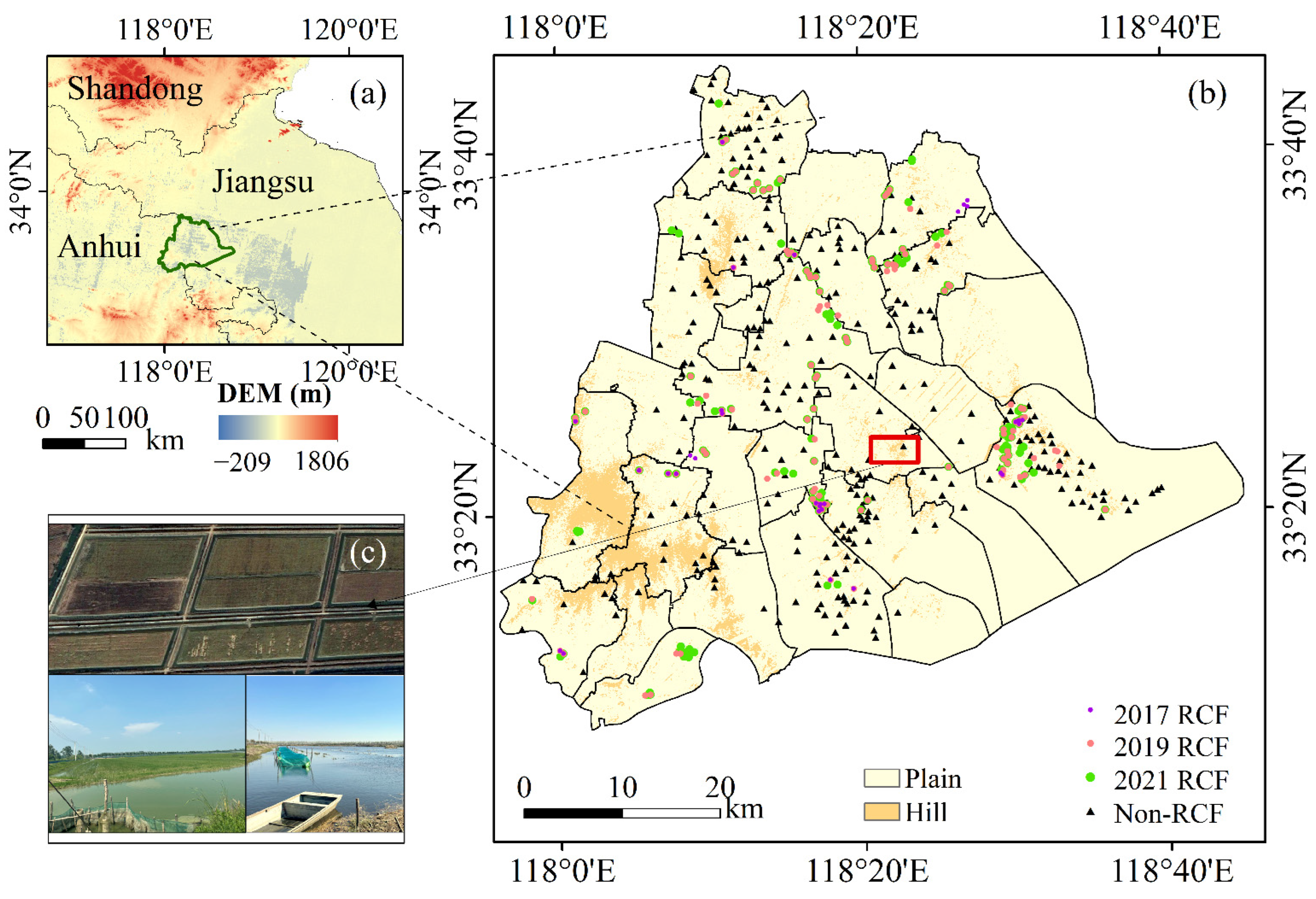
2.1. Study Area

Sihong County (117°56′–118°46′E, 33°08′–33°44′N) [25], the study area, is located in the northwestern part of Jiangsu Province, China. The terrain is dominated by plains, with scattered granite and hills distributed in the west and southwest [26]. The location of the study area and its terrain are shown in Figure 1a,b (ground elevation data from http://www.gscloud.cn, accessed on 1 March 2022). The climate type is a transition zone between the northern subtropical and temperate monsoon climate zones, as well as the East Asian monsoon zone. The local climate has four distinct seasons, with concentrated rainfall and the same seasonal pattern of rain and heat. The average yearly temperature is 14.6 °C, and the average yearly rainfall is 893.9 mm, which provide a suitable environment for agricultural development.
The two main agricultural industries in Sihong are rice cultivation and fish farming. The rice cultivation area has reached 47.85% of the county’s cropland area. For this reason, the development of the RCF pattern is highly important. The Ministry of Agriculture and Rural Affairs designated it as a “National Demonstration Area for Comprehensive Planting, Breeding, and Rice-fishing”, as there are 8 RCF bases with an area of more than 134 ha and 32 RCF bases with an area of more than 67 ha [27]. Therefore, this paper adopts Sihong County as the study area, which has a good degree of typicality.
Farmers in Sihong County farm crayfish in RCFs by digging about 4–5 m-wide and 1.5 m-deep ditches around the rice field, with safety nets installed on either side of the ditch to prevent the crayfish from escaping. The cultivation process is as follows: the addition of crayfish juveniles in April each year, the harvesting of adult crayfish from May to June, the mowing of the fields and transplantation of the rice in mid- to late June, and the planting of the rice from June to October, with the crayfish and rice growing together in the paddy fields. Therefore, the key phenological periods for RCF identification in Sihong are the rice fallow period, from April to May, and the rice growth period, from August to October, respectively (Figure 1c).

2.2. Data and Preprocessing

2.2.1. Satellite Imagery and preprocessing

In this study, Sentinel-2 MSI images (Level-2A) were selected to extract RCFs due to their high resolution and easy access. The Sentinel-2 satellite was launched by the European Space Agency (ESA), with a revisit cycle of 5 days. Additionally, it has a spatial resolution of up to 10 m and contains 13 bands [28]. We downloaded images from the ESA Copernicus Data Center (https://scihub.copernicus.eu/, accessed on 5 March 2022). In accordance with the study’s objectives, two images with appropriate timing and low cloudiness were selected to extract RCFs during two crucial phenology windows, March to May and August to October. Hence, we selected two images acquired on 1 May 2021 and 3 October 2021, respectively. The images were then resampled to a spatial resolution of 10 m using the Sentinel Application Platform (SNAP) software developed by ESA. Additionally, to verify the applicability of the construction method, the method constructed based on the 2021 data was further used to extract the RCFs in Sihong in 2017 and 2019. The principles of the image selection for 2017 and 2019 were the same as those for 2021. The specific images used are shown in Table 1. Since no high-quality images were available for the rice growth period in 2017, the Landsat-8 OLI image, whose band characteristics and spatial resolution are close to those of Sentinel-2, was selected instead. The image was downloaded from http://glovis.usgs.gov/ (accessed on 5 March 2022), fused based on the panchromatic bands, and then resampled to a 10 m resolution. The Landsat 8 image and Sentinel-2 images were geographically registered to render their spatial positions the same.

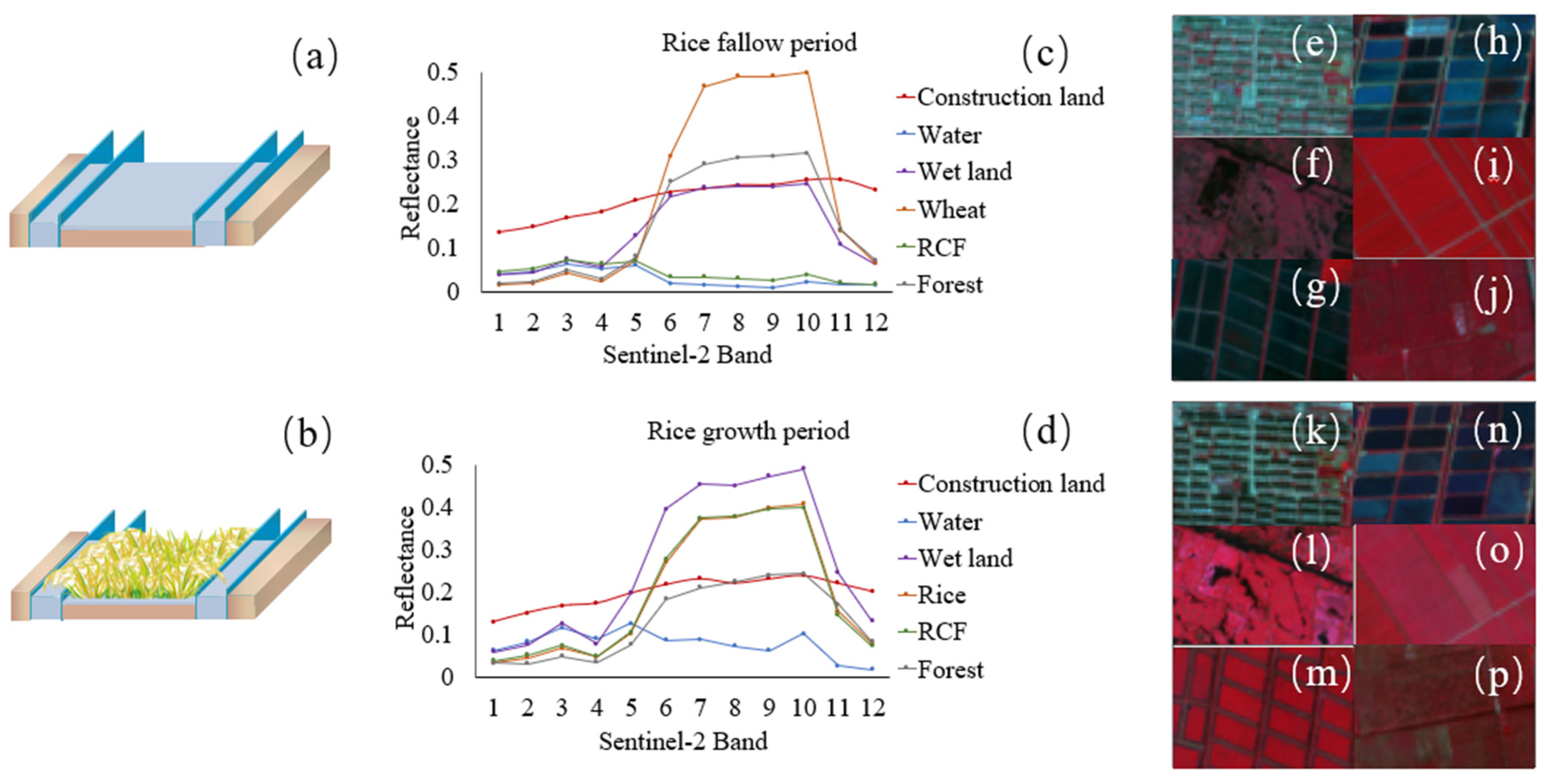
2.2.2. Ground Reference Data

The ground sample dataset was compiled using high-resolution images from the Google Earth platform and a field survey conducted in Sihong in September 2021. However, it is difficult to obtain historical samples, especially for a study area undergoing changes. Fortunately, the phenological features and field shape of RCFs are unique. The surfaces of the RCFs are covered with water during the rice fallow period and covered with rice during the rice growth period. In addition, the RCFs are composed of rice fields and surrounding ditches, creating a shape that is clearly different from that of ordinary rice fields and breeding ponds. The two abovementioned points help one to easily recognize RCFs from high-spatial-resolution satellite images. At present, the rice-crayfish system is advancing gradually in China, and the area of RCFs increased gradually from 2017 to 2021. Therefore, the historical samples were obtained by visual interpretation of high-resolution Google Earth images and a combination of Sentinel surface reflectance data with 2021 samples for reference. We judged whether the samples in 2021 had changed relative to 2017 and 2019 by simultaneously inspecting the phenological, spectral, and shape features. If changes had occurred, we dropped these points from the RCF sample data for the given year. Meanwhile, combining the abovementioned features, more RCF samples were selected to supplement the historical data (Figure 1b). In the dataset, the non-RCFs include five feature types: farming ponds, traditional rice fields, bare land, non-cultivated vegetation (forest, grassland, gardens, and wetland), and construction land. In this study, 436, 429, and 449 samples were used for the validation in 2017, 2019 and 2021, respectively.

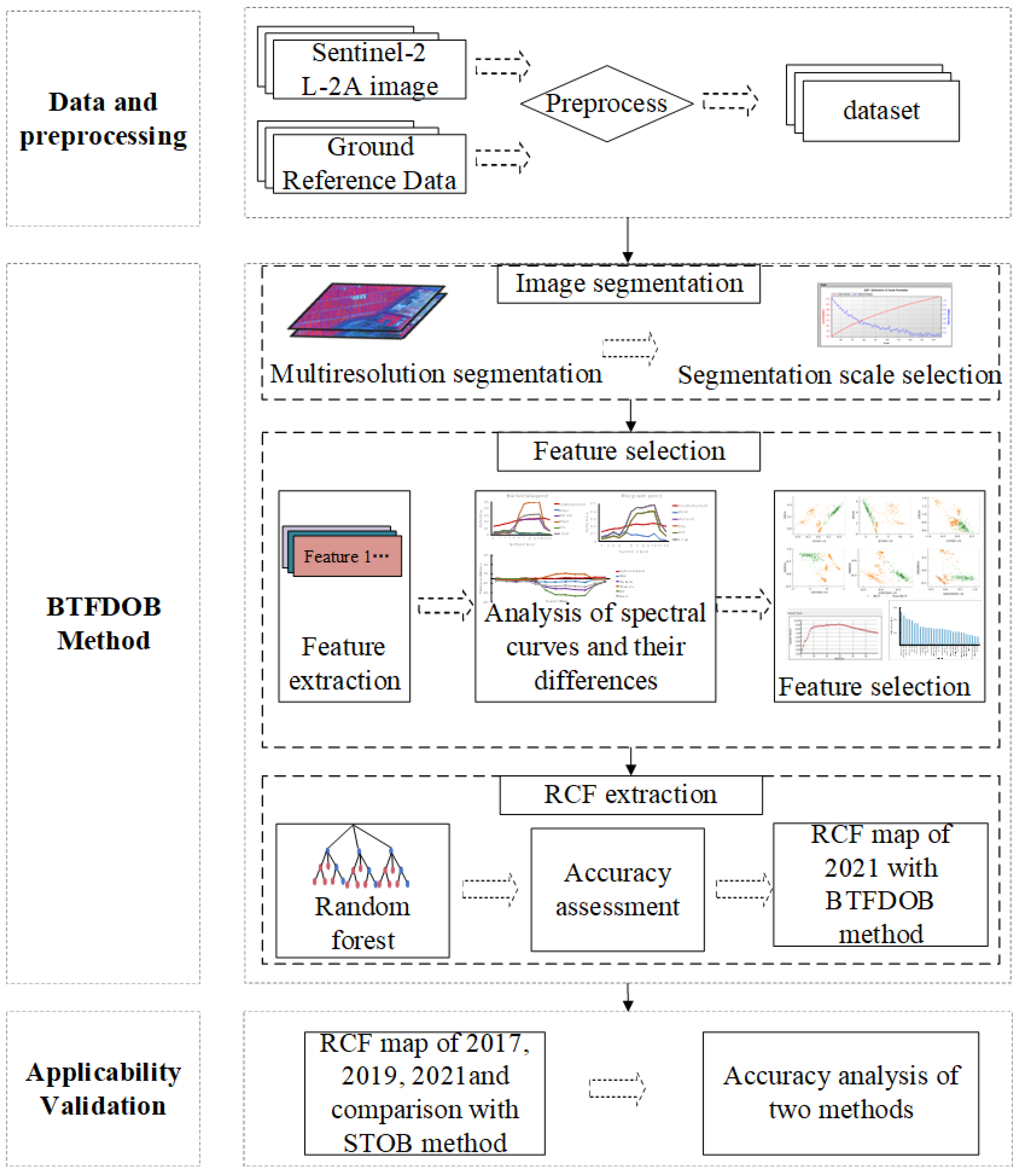
2.3. Framework of the Analysis

Based on their unique phenological features, RCFs have more water areas in the rice fallow period compared with the rice growth period. We constructed a BTFDOB method as follows: firstly, multiresolution segmentation was used to segment the images, and the optimal segmentation scales were determined by the Estimation of Scale Parameter 2 (ESP2); secondly, the features of the two images and the differences between them were selected as classification features; and subsequently, the RF classification method was used to identify each object as either RCF or non-RCF. Furthermore, the method was applied in 2019 and 2017, and the results were analyzed and compared with those of the conventional STOB approach to confirm their applicability. Figure 2 displays the overall flowchart of the study.

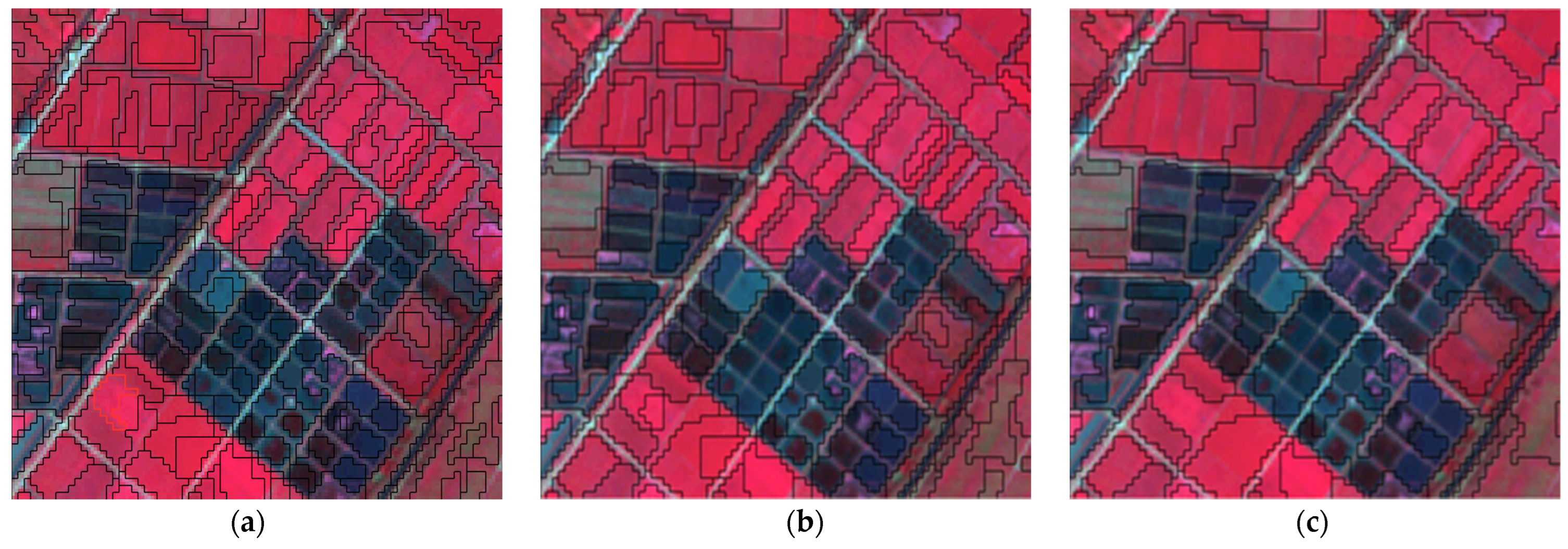
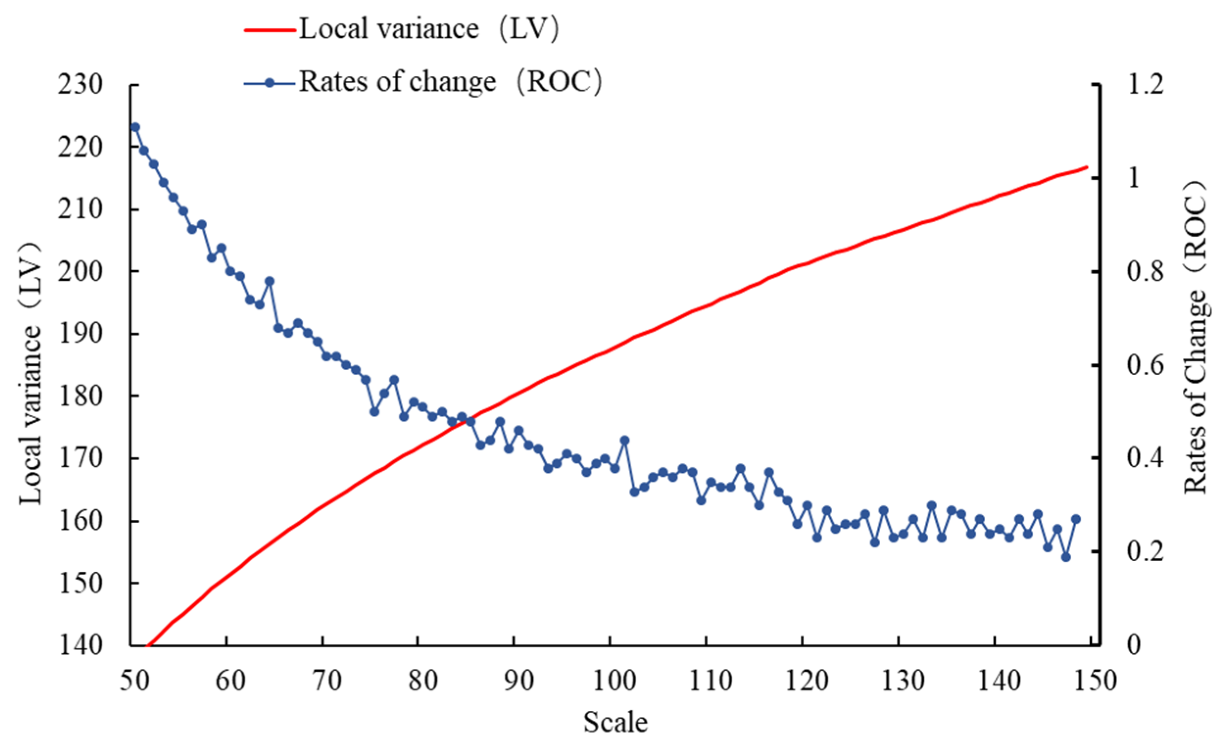
2.3.1. Segmentation Method

The images were segmented using the multiscale segmentation algorithm embedded in the eCognition software, which has been widely applied for high-resolution image classification and significantly increased the classification accuracy in comparison to other segmentation algorithms [29,30]. The three crucial parameters for image segmentation in this algorithm are the scale, shape, and compactness [31]. ESP2 was adopted to select the optimal segmentation scale. This tool iteratively produces image objects of numerous scale levels from the bottom up and calculates the local variation (LV) in the image object homogeneity under different segmentation scale settings to decide which one is optimal [32]. The threshold of the rate of change (ROC) curve of the LV (ROC-LV) indicates the scale level at which the image can be segmented most appropriately [33].

2.3.2. Feature Selection

The spectral properties of different objects, such as the cultivated land, water, and construction land, vary greatly. The high-resolution images are rich in texture information and geometric information, which can be effectively used to distinguish roads and other objects. Concerning the research purpose and the feature type of the study area, the spectral features, texture features, and geometric features of the bi-temporal images were extracted as the initial feature space. Based on this, we selected 20 spectral features, 5 texture features, and 4 geometric features for each of the two images, as shown in Table 2.

2.3.3. RF Classification

RF is an ensemble learning method proposed by Breiman to solve both classification and regression problems [41], which is widely used in remote sensing image classification [42]. Compared with the support vector machine (SVM) and decision tree (DT) methods, the RF method is less sensitive to feature selection and can also obtain better classification results when handling multi-dimensional data, such as hyperspectral or multi-source data [42]. Sihong is mainly covered by cropland, with a more concentrated crop distribution and less intercropping. It has been shown that the accuracy of the RF method in cropland classification is higher than that of the SVM method [43]. Therefore, we selected the RF method. The number of features contained in each decision tree and the number of decision trees are important parameters of the RF method. In this study, the number of features of each decision tree equaled the number of optimal features, and the number of decision trees selected by the Grid-Search CV was 97.

2.3.4. Validation to Evaluate the BTFCOB Method

Two types of validation methods were used in the accuracy assessment. Firstly, the error matrix, based on the training and test area (TTA) masking approach embedded in eCognition, was selected for the classification accuracy assessment. This method can effectively reduce the influences of human factors, and for this reason, it is widely used for the accuracy evaluation of object-based classification results [44,45,46]. The overall accuracy (OA), producer’s accuracy (PA), user’s accuracy (UA), and Kappa coefficient in the confusion matrix were important parameters for the accuracy evaluation of our classification results. Secondly, to further analyze the potential of the BTFDOB method, the classification results were compared with those of the traditional STOB method for RCF extraction. The STOB method classified the two images from each year separately. The classification results of the two periods were compared, and the parts with reduced water were identified as RCFs. The method also used an object-based approach to segment the images and classified them using an RF method.

3. Results

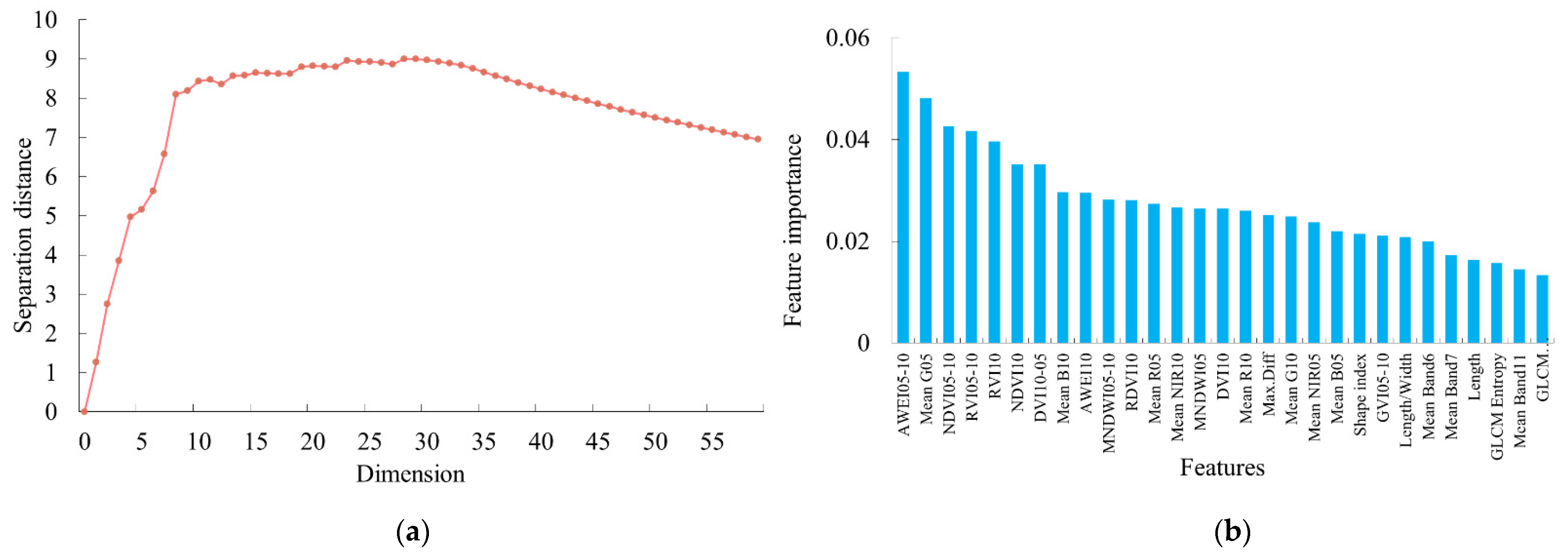
3.1. Determination of the Optimal Segmentation Scale

We investigated the optimal segmentation scale for the cultivated land and aquaculture water surface using the multiresolution segmentation method. To examine the impact of the segmentation scale on the segmentation results, the shape and compactness were set to 0.1 and 0.5, respectively, and the segmentation scale range was set to 50–200, with a segmentation layer generated every 25 (Figure 3). After setting the segmentation scale to 100 or above, several areas of cropland or ponds were merged into one object. Therefore, the segmentation scale over 100 was excluded. When the segmentation scale was 50, many objects that should have been merged remained as small units. The scale of segmentation of 75 was suitable for the classification.
Then, we set the segmentation scale to 75 and explored how the shape and compactness affected the segmentation results. The compactness was set to 0.5 and the shape factor was set to 0.1–0.5. The results showed that when the shape was 0.4, the segmentation effect was optimal. Therefore, we determined the shape to be 0.4 and further compared the segmentation effect with the compactness of 0.4–0.8, yielding a result of 0.6.
Next, we used the ESP2 tool to objectively select the segmentation scale (Figure 4). The optimal segmentation scale corresponded to the peak of the LV change rate. The segmentation scale ranged from 50 to 100, and the segmentation scales corresponding to the LV peak were 65, 78, 80, 89, 91, and 100. Judging by sight, when the segmentation scale was 80, the segmentation effect was the best; thus, we determined that the optimal segmentation scale was 80.

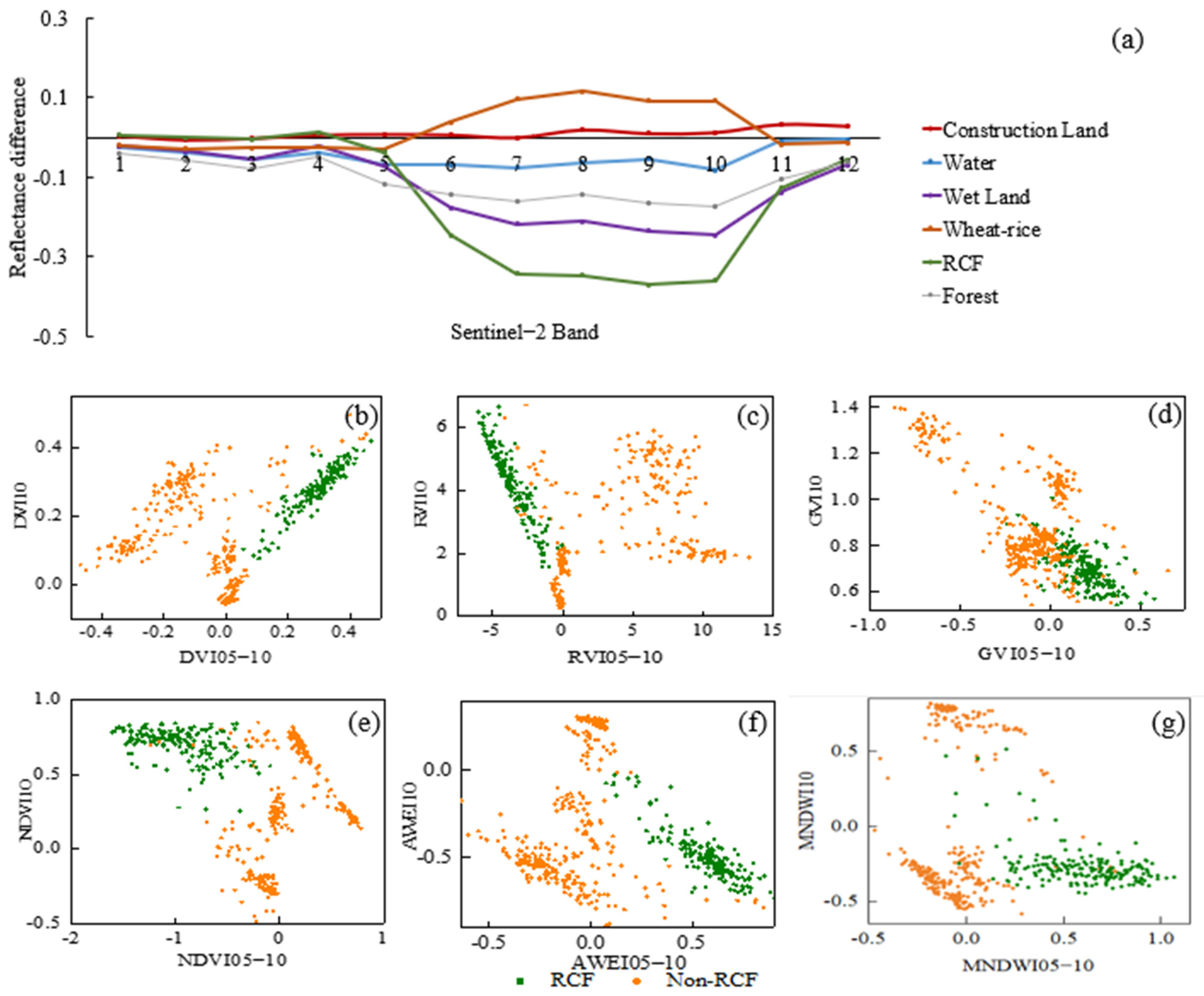
3.2. Feature Selection of the BTFDOB Method

The analysis of spectral information is a key step in classification. The RCFs were flooded in the rice fallow period, as shown in Figure 5a, and the rice was planted in the rice growth period, as shown in Figure 5b. We calculated the average spectral reflectance of each training sample for six major ground objects in two critical periods: construction land, water, wetland, forest, normal rice fields (wheat during the rice field fallow period), and RCFs. Figure 5c,d illustrates the spectral curves of the different land cover types during the two periods. Except for the construction land, the spectral curves of the other objects in the two periods were similar in three bands (red, green, and blue) but notably different in bands 6–10. In the rice fallow period, the RCFs were flooded with water, which resulted in an analogous spectral response indicating water with a lower SWIR1 and SWIR2 reflectance compared with the others (Figure 5c). Meanwhile, in the rice growth period, the RCFs had a similar spectral curve to the normal rice fields (Figure 5d). The false-color Sentinel-2 images of the six categories of objects in the two periods are shown in Figure 5e–p. During the rice fallow period, the appearance of the RCFs was no different from that of the ponds, as shown in Figure 5g, while during the rice growth period, the RCFs and normal rice fields were both red, as shown in Figure 5m. Therefore, the periodic spectral feature changes in the RCFs were the key to their identification.
Based on the above analysis, we calculated and plotted the spectral reflectance difference between the RCFs and non-RCFs for each band in both periods. The spectral reflectance difference between the RCFs and the other non-RCFs was significant in band 4 and bands 6 to 10, as shown in Figure 6a. Then, we calculated the differences in the vegetation indices in the abovementioned bands of the RCFs and non-RCFs between the two periods and plotted their two-dimensional scatter plots with the associated October vegetation indices (Figure 6b–g). The result suggested that the two land cover types exhibited significant differences. Thus, the above differences in the vegetation indices were added to the initial feature set as classification features.
Feature optimization is required to avoid information redundancy and classification efficiency reduction due to the excessive number of features involved in classification. All features in the initial feature space were calculated using the eCognition software feature analysis tool. The number of features in the optimal feature set and their corresponding top-ranked features are shown in Figure 7. We observed that the separation distance increased rapidly as the number of features increased, hitting a peak when the number of features was 29 and then dropping steadily as the number of features increased further, demonstrating that redundant features diminish the classification accuracy. Finally, we determined the number of optimal features to be 29, and the features used in the RF classification were the top 29 features in terms of the feature importance, as shown in Figure 7. In addition, when distinguishing the RCFs from the non-RCFs, the importance of the spectral features is generally higher than that of the texture features and geometric features. The importance scores of the vegetation index differences, such as the AWEI, NDVI, RVI, MNDWI, and GVI, were higher. GLCM Entropy and GLCM Homogeneity received greater scores among the texture characteristics, whereas the shape index and length/width were ranked higher in importance among the geometric features.

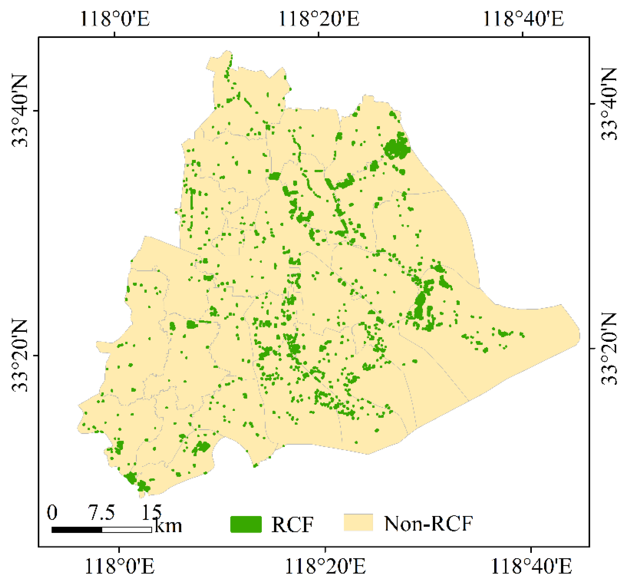
3.3. RCF Extraction and Accuracy Assessment of 2021

Using the BTFDOB method, we extracted the RCFs of Sihong in 2021 (Figure 8). The RCFs were primarily distributed in the eastern and southern plain areas, which have a well-developed water system for rice cultivation and are thus suitable for planting RCFs, while they were rarely distributed in the hilly areas. Using the TTA masking method, the accuracy of the classification results was evaluated (Table 3). The PA and the UA of the RCFs were 93.93% and 91.76%, respectively. The OA of the classification was 96.77%, and the Kappa coefficient was 0.92.

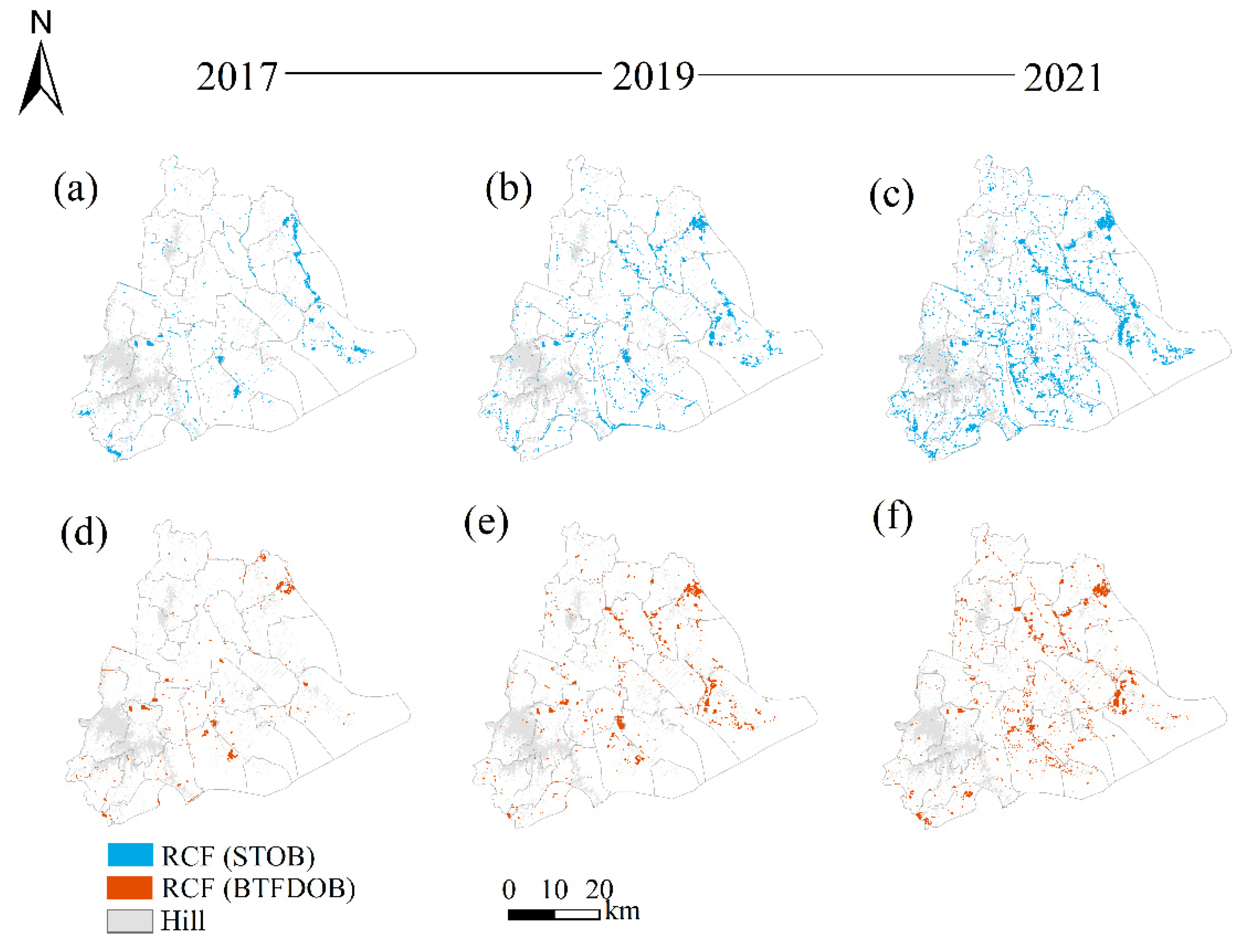
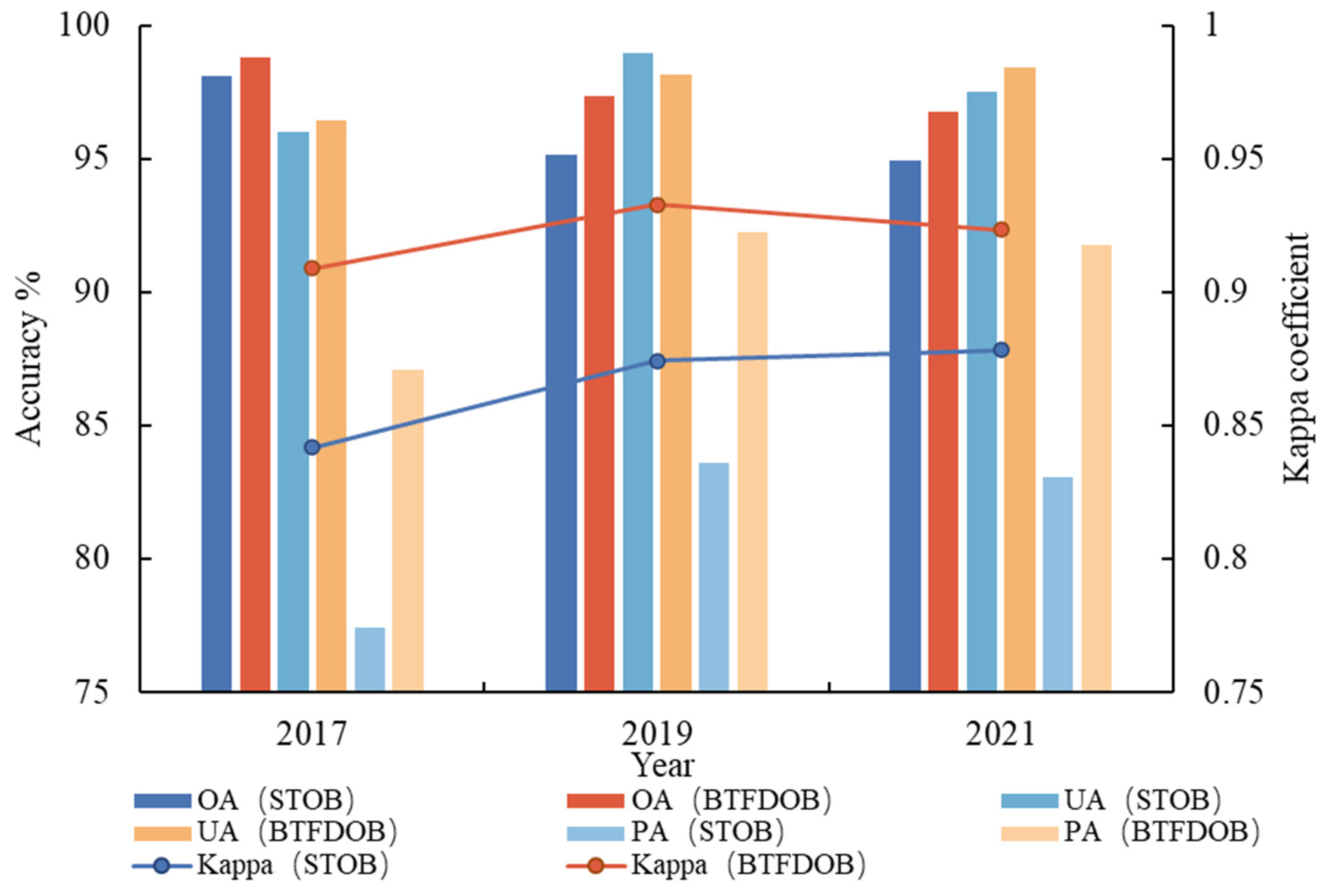
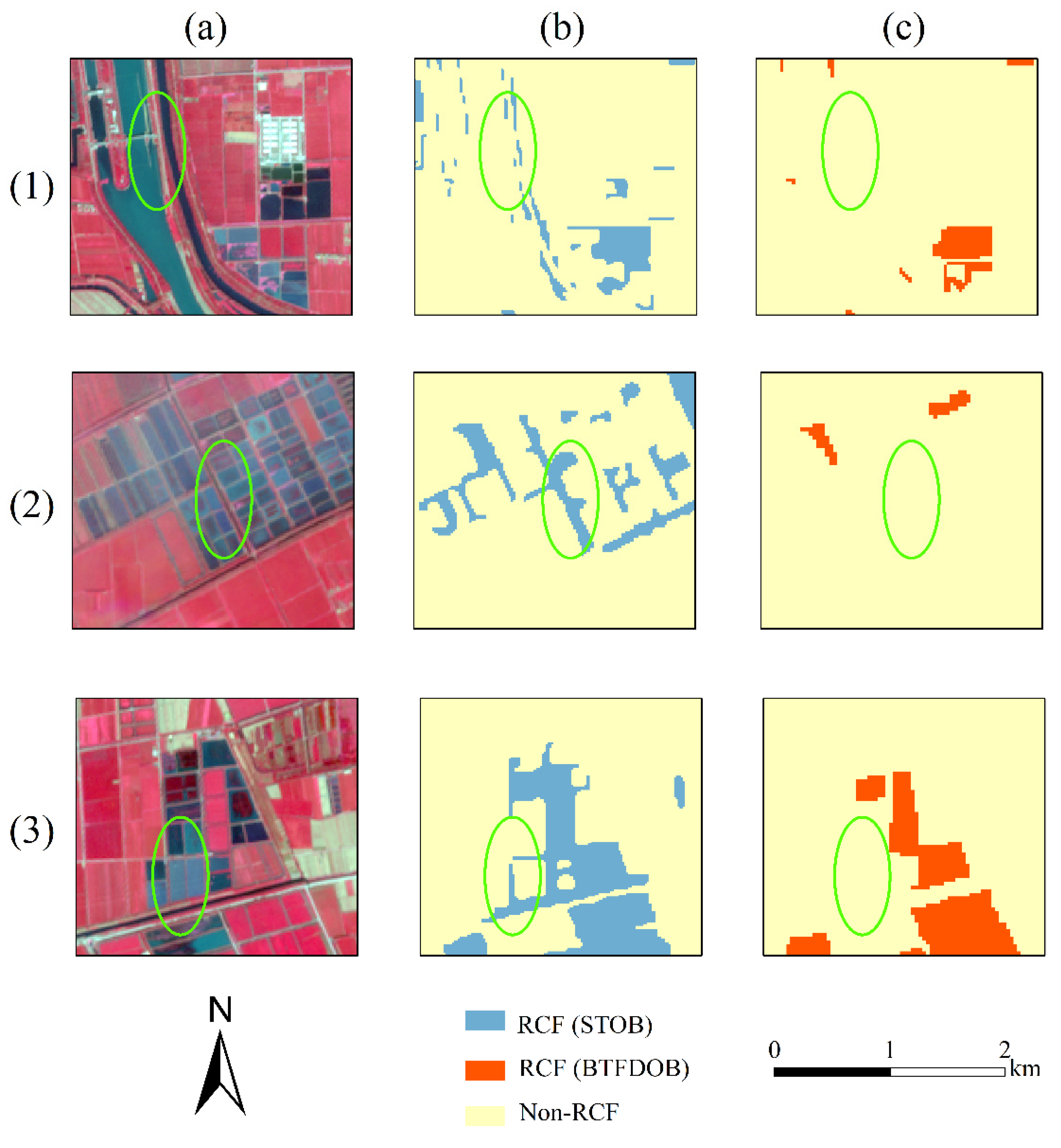
3.4. Comparison with the STOB Method Based on Three Years

We applied the BTFDOB method to the data of 2017 and 2019 and compared it with the conventional STOB method to test its applicability. The RCF maps obtained by the two methods are shown in Figure 9. We observed that only some scattered experimental areas operated with a rice-crayfish system in 2017. With the success of the experimental areas and the development of agricultural technology, the scale of this system has continued to expand. The rice-crayfish system has now been promoted throughout the county. The RCFs identified by the two methods were mainly distributed in the eastern and southern areas, while they were rarely distributed in the hilly areas with mainly dry farming.
The accuracy of the classification results of both methods was verified (Figure 10). The results showed that both methods had high OA and Kappa coefficients, with the BTFDOB method having a higher OA and Kappa coefficient than the STOB method, indicating the better applicability of the BTFDOB method. The BTFDOB method had a considerably higher PA than STOB, suggesting that there were fewer omission errors in the extraction of the RCFs based on the BTFDOB method. The UA of the BTFDOB method was higher in 2017 and 2021 than in 2019, indicating that the method had fewer misclassification errors.
We calculated the area of RCFs. The total area of the RCFs in Sihong County was 1240.26 ha, 2885.90 ha, and 3495.68 ha in 2017, 2019, and 2021, respectively.

4. Discussion

4.1. Advantages of the BTFDOB Method

Land cover variations in the RCFs over the two periods resulted in significant changes in the spectral features of the bi-temporal images. Therefore, the method was used to analyze the reflectance changes in each band of the RCFs and non-RCFs over the two periods, thereby strengthening the link between the bi-temporal images. In the red band, the spectral characteristics of the cropland show strong absorption, so that the difference in the reflectivity of the RCFs between the two periods has a small peak in this band. In the red-edge band and NIR band, the water has strong absorption, while the internal structure of the rice leaves in these bands show high reflectivity, rendering it easier to distinguish the RCFs in these two bands [47,48]. The vegetation index differences indicated by these different bands were introduced as classification features. The result of the feature selection also shows that these feature differences have a high importance score, which verifies the results shown in Figure 6. In addition, the high-resolution images are information rich, and the object-based classification method can eliminate the influences of the phenomena of both ‘similar spectral information from different objects’ and ‘different spectral information from similar objects’.
Previously, a land use transfer matrix was used to identify RCFs based on only two single-temporal classification results [14,15,20]. In this method, the accuracy of the STOB classification is affected by the accuracy of the two single-temporal classification results. Since the two images are not segmented simultaneously, the STOB method mixes the RCFs with the marginal pixels of wetlands or rivers and lakes, generating unavoidable errors [49]. The STOB method causes the errors generated in the classification process to eventually accumulate, affecting the accuracy of the change detection results. Compared with STOB, the BTFDOB method segments the bi-temporal images simultaneously to ensure that the edges of the objects are consistent. Taking several typical regions as examples (Figure 11) with the Sentinel-2 zoomed-in image from October 2021 for comparison, we can see that, at this time, the areas shown as water in column (a) of the figure were all non-RCFs. We can determine that the edge pixels of the breeding pond objects and water objects were misclassified as RCFs by the STOB method. However, such errors did not appear when using the BTFDOB method, which can effectively circumvent this drawback.
In addition, the surface covering of the RCFs varies with the seasons; thus, their identification can be regarded as the identification of changing areas. The BTFDOB method takes into account the influences of feature differences on the change detection. In the past, the post-classification comparison method and image transformation method were used for change detection. The accuracy of the former is based on the classification accuracy of the two images, respectively [50,51]. The latter extracts the respective features from the two phases for comparison in order to detect the change and does not maximize the difference between the two periods [52,53]. The BTFDOB method can compensate for the defects of the above two methods.

4.2. Potential of the BTFDOB Method

Defining the key phenological period of the RCFs is the first step in their identification. There is no obvious difference in the spectral and texture features between the RCFs and normal rice fields during the rice growth period. Meanwhile, no distinct difference between the RCFs and breeding ponds exists during the rice-field fallow period. Therefore, most of the prior studies extracted the RCFs based on the seasonal differences in the water area. The farming system in Sihong County is rice–wheat rotation or corn–wheat rotation, of which rice is a single-cropping product [54]. When selecting the images of the rice field fallow period, the field investigation and the comparison of the images after rice harvesting from March, May, and December revealed that all the RCFs were flooded only in May, in contrast to Qianjiang. In South and Southwest China and other regions, the planting structure is complex, and double-cropping rice is widely utilized. The local RCF system generates rice and crayfish twice in one year [55]. When the BTFDOB method is applied to these areas, it is necessary to define the key local phenology and select images from the appropriate period.

4.3. Accuracy Improvements

In this paper, we identified the areas that were transformed from water to cropland as RCFs. Due to the uniform local cultivation seasons, a few RCFs remained unidentified due to phenological differences, resulting in minor errors. In response to this problem, time series images could be applied to study the feature differences throughout the whole year so as to improve the classification accuracy.
We used Sentinel-2 images with a spatial resolution of 10 m as data. However, optical images are easily influenced by meteorological conditions, such as cloud and rain. Therefore, it is possible that images of the appropriate phenological periods will be missing or that the time window suitable for extracting the RCFs will not produce high quality images. Synthetic aperture radar (SAR) can penetrate clouds and rain, compensating for the deficiency of optical images affected by clouds and rain in the second quarter. Therefore, it can be adopted to monitor the dynamic changes in cropland [56,57]. In future work, we will consider optical images in conjunction with SAR images to identify RCFs. Furthermore, the spatial resolution of the remote sensing data is generally greater than the width of the surrounding ditch, which means that these mixed pixels are identified as non-RCFs. Therefore, much effort will be required to collect higher-spatial-resolution images or decompose mixed pixels in time.

5. Conclusions

Mapping RCFs and identifying them from pure rice fields are challenging due to their spectral similarity and complexity. In this paper, we proposed a BTFDOB method to achieve the above purposes. This method combined the bi-temporal-feature-differences with object-based method for mapping RCFs in Sihong County. We adopted BTFDOB method and STOB method to carry out the experiments in different years. By comparing the results of the two methods, we found that the BTFDOB method performed better than the STOB method in identifying the RCFs. The use of the bi-temporal-feature-differences as classification feature yielded a higher accuracy in mapping RCFs, with an OA improvement of up to 2.18%. We discussed the importance of each feature in detail. We found that compared with the geometric features and texture features, the spectral features of the bi-temporal images, especially the spectral feature differences, were the most important features in the feature set.
In addition, the method provided a new method for the detection of the change regions of two periods. It widened the difference between the changing and non-changing regions and improved the detection accuracy.
In this study, by adopting the BTFDOB method, we systematically analyzed the possibility of conducting RCF identification in Sihong County, which have applications such as planting structure optimization and crop yield prediction. In future research, time-series images and new data sources should be considered.

Author Contributions

Conceptualization, S.M. and Z.L.; methodology, S.M. and D.W.; software, S.M.; validation, S.M. and D.W.; formal analysis, S.M. and H.Y.; investigation, C.L. and H.Y.; resources, C.L., H.H. and H.Y.; data curation, H.H.; writing—original draft preparation, S.M.; writing—review and editing, D.W., C.L. and Z.L.; visualization, S.M.; supervision, Z.L.; project administration, Z.L.; funding acquisition, Z.L. All authors have read and agreed to the published version of the manuscript.

Funding

This research was funded by the Jiangsu Provincial Key Research and Development Program, grant number BE2019386.

Data Availability Statement

Not applicable.

Conflicts of Interest

The authors declare no conflict of interest.

References

  1. Du, F.; Hua, L.; Zhai, L.; Zhang, F.; Fan, X.; Wang, S.; Liu, Y.; Liu, H. Rice-crayfish pattern in irrigation-drainage unit increased N runoff losses and facilitated N enrichment in ditches. Sci. Total Environ. 2022, 848, 157721. [Google Scholar] [CrossRef] [PubMed]
  2. Jiang, Y.; Cao, C. Crayfish–rice integrated system of production: An agriculture success story in China. A review. Agron. Sustain. Dev. 2021, 41, 68. [Google Scholar] [CrossRef]
  3. Xu, Q.; Liu, T.; Guo, H.L.; Duo, Z.; Gao, H.; Zhang, H.C. Conversion from rice-wheat rotation to rice-crayfish coculture increases net ecosystem service values in Hung-tse Lake area, east China. J. Clean. Prod. 2021, 319, 128883. [Google Scholar] [CrossRef]
  4. Xu, Q.; Peng, X.; Guo, H.L.; Che, Y.; Dou, Z.; Xing, Z.P.; Hou, J.; Styles, D.; Gao, H.; Zhang, H.C. Rice-crayfish coculture delivers more nutrition at a lower environmental cost. Sustain. Prod. Consum. 2022, 29, 14–24. [Google Scholar] [CrossRef]
  5. Hou, J.; Wang, X.L.; Xu, Q.; Cao, Y.X.; Zhang, D.Y.; Zhu, J.Q. Rice-crayfish systems are not a panacea for sustaining cleaner food production. Environ. Sci. Pollut. Res. 2021, 28, 22913–22926. [Google Scholar] [CrossRef]
  6. Mo, A.J.; Dang, Y.; Wang, J.H.; Liu, C.S.; Yang, H.J.; Zhai, Y.X.; Wang, Y.S.; Yuan, Y.C. Heavy metal residues, releases and food health risks between the two main crayfish culturing models: Rice-crayfish coculture system versus crayfish intensive culture system. Environ. Pollut. 2022, 305, 119216. [Google Scholar] [CrossRef]
  7. Yuan, J.; Liao, C.A.S.; Zhang, T.L.; Guo, C.A.B.; Liu, J.S. Advances in ecology research on integrated rice field aquaculture in China. Water 2022, 14, 2333. [Google Scholar] [CrossRef]
  8. Anastacio, P.M.; Parente, V.S.; Correia, A.M. Crayfish effects on seeds and seedlings: Identification and quantification of damage. Freshw. Biol. 2005, 50, 697–704. [Google Scholar] [CrossRef]
  9. Gedik, K.; Kongchum, M.; DeLaune, R.D.; Sonnier, J.J. Distribution of arsenic and other metals in crayfish tissues (Procambarus clarkii) under different production practices. Sci. Total Environ. 2017, 574, 322–331. [Google Scholar] [CrossRef]
  10. Li, B.L.; Peng, S.B.; Shen, R.P.; Yang, Z.L.; Yan, X.Y.; Li, X.F.; Li, R.R.; Li, C.Y.; Zhang, G.B. Development of a new index for automated mapping of ratoon rice areas using time-series normalized difference vegetation index imagery. Pedosphere 2022, 32, 576–587. [Google Scholar] [CrossRef]
  11. Mahlayeye, M.; Darvishzadeh, R.; Nelson, A. Cropping patterns of annual crops: A remote sensing review. Remote Sens. 2022, 14, 2404. [Google Scholar] [CrossRef]
  12. Chabalala, Y.; Adam, E.; Ali, K.A. Machine learning classification of fused Sentinel-1 and Sentinel-2 image data towards mapping fruit plantations in highly heterogenous landscapes. Remote Sens. 2022, 14, 2621. [Google Scholar] [CrossRef]
  13. Wei, H.D.; Hu, Q.; Cai, Z.W.; Yang, J.Y.; Song, Q.; Yin, G.F.; Xu, B.D. An Object- and Topology-Based Analysis (OTBA) Method for Mapping Rice-Crayfish Fields in South China. Remote Sens. 2021, 13, 4666. [Google Scholar] [CrossRef]
  14. Wei, Y.; Lu, M.; Yu, Q.; Xie, A.; Hu, Q.; Wu, W. Understanding the dynamics of integrated rice-crawfish farming in Qianjiang county, China using Landsat time series images. Agric. Syst. 2021, 191, 103167. [Google Scholar] [CrossRef]
  15. Chen, Y.L.; Yu, P.H.; Chen, Y.Y.; Chen, Z.Y. Spatiotemporal dynamics of rice-crayfish field in Mid-China and its socioeconomic benefits on rural revitalisation. Appl. Geogr. 2022, 139, 102636. [Google Scholar] [CrossRef]
  16. Belgiu, M.; Csillik, O. Sentinel-2 cropland mapping using pixel-based and object-based time-weighted dynamic time warping analysis. Remote Sens. Environ. 2018, 204, 509–523. [Google Scholar] [CrossRef]
  17. Yan, Z.Y.; Ma, L.; He, W.Q.; Zhou, L.; Lu, H.; Liu, G.; Huang, G.A. Comparing Object-Based and Pixel-Based Methods for Local Climate Zones Mapping with Multi-Source Data. Remote Sens. 2022, 14, 3744. [Google Scholar] [CrossRef]
  18. Song, Q.; Hu, Q.; Zhou, Q.; Hovis, C.; Xiang, M.; Tang, H.; Wu, W. In-season crop mapping with GF-1/WFV data by combining object-based image analysis and Random Forest. Remote Sens. 2017, 9, 1184. [Google Scholar] [CrossRef] [Green Version]
  19. Karimi, N.; Sheshangosht, S.; Eftekhari, M. Crop type detection using an object-based classification method and multi-temporal Landsat satellite images. Paddy Water Environ. 2022, 20, 395–412. [Google Scholar] [CrossRef]
  20. Xia, T.; Ji, W.; Li, W.; Zhang, C.; Wu, W. Phenology-based decision tree classification of rice-crayfish fields from Sentinel-2 imagery in Qianjiang, China. Int. J. Remote Sens. 2021, 42, 8124–8144. [Google Scholar] [CrossRef]
  21. Li, L.; Li, X.; Zhang, Y.; Wang, L.; Ying, G. Change detection for high-resolution remote sensing imagery using object-oriented change vector analysis method. In Proceedings of the 36th IEEE International Geoscience and Remote Sensing Symposium (IGARSS), Beijing, China, 10–15 July 2016; pp. 2873–2876. [Google Scholar] [CrossRef]
  22. Ge, C.; Ding, H.; Molina, I.; He, Y.; Peng, D. Object-oriented change detection method based on spectral-spatial-saliency change information and fuzzy integral decision fusion for hr remote sensing images. Remote Sens. 2022, 14, 3297. [Google Scholar] [CrossRef]
  23. Huang, Q.; Meng, Y.; Chen, J.; Yue, A.; Lin, L. Landslide change detection based on spatio-temporal context. In Proceedings of the IEEE International Geoscience & Remote Sensing Symposium, Fort Worth, TX, USA, 23–28 July 2017; pp. 1095–1098. [Google Scholar] [CrossRef]
  24. National Aquatic Technology Extension Station of the People’s Republic of China. Report on the Industry Development of China’s Integrated Rice-fish Farming (2020). China Fish. 2020, 10, 12–19. Available online: https://kns.cnki.net/kns8/Detail?sfield=fn&QueryID=4&CurRec=5&recid=&FileName=SICA202107013&DbName=CJFDLAST2021&DbCode=CJFD&yx=&pr=&URLID= (accessed on 16 January 2022). (In Chinese).
  25. Chen, G.; Chen, Y.; Yu, H.; Zhou, L.; Zhuang, X. Accumulated temperature requirements of Echinochloa crus-galli seed-setting: A case study with populations collected from rice fields. Weed Biol. Manag. 2022, 22, 47–55. [Google Scholar] [CrossRef]
  26. Jiang, J.; Zhang, Z.; Cao, Q.; Liang, Y.; Krienke, B.; Tian, Y.; Zhu, Y.; Cao, W.; Liu, X. Use of an active canopy sensor mounted on an unmanned aerial vehicle to monitor the growth and nitrogen status of winter wheat. Remote Sens. 2020, 12, 3684. [Google Scholar] [CrossRef]
  27. Wang, S.; Mo, G.; Sun, X.; Gong, Z.; Wang, Y. Development report of rice and fishery comprehensive planting and breeding industry in Sihong County, Jiangsu Province. Fish. Guide Be Rich 2021, 13, 13–18. Available online: https://kns.cnki.net/kcms/detail/detail.aspx?dbcode=CJFD&dbname=CJFDLAST2021&filename=YYZF202113006&uniplatform=NZKPT&v=SkjwbWSNHEZvJmLwHyBcyBhwPONcAeAUUGets6AOCMyaFM-l0FaJvOm_vQUsGlrc (accessed on 17 January 2022). (In Chinese).
  28. Rodriguez-Lopez, L.; Gonzalez-Rodriguez, L.; Duran-Llacer, I.; Garcia, W.; Cardenas, R.; Urrutia, R. Assessment of the diffuse attenuation coefficient of photosynthetically active radiation in a Chilean Lake. Remote Sens. 2022, 14, 4568. [Google Scholar] [CrossRef]
  29. Zhang, X.L.; Xiao, P.F.; Feng, X.Z.; Feng, L.; Ye, N. Toward evaluating multiscale segmentations of high spatial resolution remote sensing images. IEEE Trans. Geosci. Remote Sens. 2015, 53, 3694–3706. [Google Scholar] [CrossRef]
  30. Li, P.J.; Xiao, X.B. Evaluation of multiscale morphological segmentation of multispectral imagery for land cover classification. In Proceedings of the IEEE International Geoscience and Remote Sensing Symposium, Anchorage, AK, USA, 20–24 September 2004; pp. 2676–2679. [Google Scholar] [CrossRef]
  31. Shen, Y.; Chen, J.; Xiao, L.; Pan, D. Optimizing multiscale segmentation with local spectral heterogeneity measure for high resolution remote sensing images. ISPRS J. Photogramm. Remote Sens. 2019, 157, 13–25. [Google Scholar] [CrossRef]
  32. Dragut, L.; Tiede, D.; Levick, S.R. ESP: A tool to estimate scale parameter for multiresolution image segmentation of remotely sensed data. Int. J. Geogr. Inf. Sci. 2010, 24, 859–871. [Google Scholar] [CrossRef] [Green Version]
  33. d’Oleire-Oltmanns, S.; Eisank, C.; Dragut, L.; Blaschke, T. An object-based workflow to extract landforms at multiple scales from two distinct data types. IEEE Geosci. Remote Sens. Lett. 2013, 10, 947–951. [Google Scholar] [CrossRef]
  34. Trimble. eCognition Developer 9.0.1 Reference Book; Trimble Germany GmbH: Munich, Germany, 2014; Available online: https://scholar.google.com/scholar_lookup?title=eCognition+Developer+9.0.1+Reference+Book&author=Trimble&publication_year=2014 (accessed on 12 March 2022).
  35. Feyisa, G.L.; Meilby, H.; Fensholt, R.; Proud, S.R. Automated Water Extraction Index: A new technique for surface water mapping using Landsat imagery. Remote Sens. Environ. 2014, 140, 23–35. [Google Scholar] [CrossRef]
  36. Huete, A.; Didan, K.; Miura, T.; Rodriguez, E.P.; Gao, X.; Ferreira, L.G. Overview of the radiometric and biophysical performance of the MODIS vegetation indices. Remote Sens. Environ. 2002, 83, 195–213. [Google Scholar] [CrossRef]
  37. Naji, T.A.H. Study of vegetation cover distribution using DVI, PVI, WDVI indices with 2D-space plot. In Proceedings of the Ibn Al-Haitham 1st International Scientific Conference on Biology, Chemistry, Computer Science, Mathematics, and Physics (IHSCICONF), Baghdad, Iraq, 13–14 December 2017. [Google Scholar] [CrossRef]
  38. Bilgili, B.C.; Satir, O.; Muftuoglu, V.; Ozyavuz, M. A simplified method for the determination and monitoring of green areas in urban parks using multispectral vegetation indices. J. Environ. Prot. Ecol. 2014, 15, 1059–1065. Available online: https://scholar.google.com/scholar?hl=zh-CN&as_sdt=0%2C5&q=A+simplified+method+for+the+determination+and+monitoring+of+green+areas+in+urban+parks+using+multispectral+vegetation+indices&btnG= (accessed on 17 May 2022).
  39. Yang, F.; Liu, T.; Wang, Q.; Du, M.; Yang, T.; Liu, D.; Li, S.; Liu, S. Rapid determination of leaf water content for monitoring waterlogging in winter wheat based on hyperspectral parameters. J. Integr. Agric. 2021, 20, 2613–2626. [Google Scholar] [CrossRef]
  40. Stehman, S.V. Sampling designs for accuracy assessment of land cover. Int. J. Remote Sens. 2009, 30, 5243–5272. [Google Scholar] [CrossRef]
  41. Breiman, L. Random forests. Mach. Learn. 2001, 45, 5–32. [Google Scholar] [CrossRef] [Green Version]
  42. Belgiu, M.; Dragut, L. Random forest in remote sensing: A review of applications and future directions. Isprs J. Photogramm. Remote Sens. 2016, 114, 24–31. [Google Scholar] [CrossRef]
  43. Sheykhmousa, M.; Mahdianpari, M.; Ghanbari, H.; Mohammadimanesh, F.; Ghamisi, P.; Homayouni, S. Support Vector Machine Versus Random Forest for Remote Sensing Image Classification: A Meta-Analysis and Systematic Review. IEEE J. Sel. Top. Appl. Earth Obs. Remote Sens. 2020, 13, 6308–6325. [Google Scholar] [CrossRef]
  44. Sol’anka, J.; Kurcikova, M.; Chudy, F.; Sgem. Automatic classification of forest stand boundaries based on results of aerial photogrammetry. In Proceedings of the 14th International Multidisciplinary Scientific Geoconference (SGEM), Albena, Bulgaria, 17–26 June 2014; p. 55. Available online: https://scholar.google.com/scholar?hl=zh-CN&as_sdt=0%2C5&q=Automatic+classification+of+forest+stand+boundaries+based+on+results+of+aerial+photogrammetry&btnG= (accessed on 21 May 2022).
  45. Lavreniuk, M.; Kussul, N.; Shelestov, A.; Dubovyk, O.; Low, F. Object-based postprocessing method for crop classification maps. In Proceedings of the 38th IEEE International Geoscience and Remote Sensing Symposium (IGARSS), Valencia, Spain, 22–27 July 2018; pp. 7058–7061. [Google Scholar] [CrossRef]
  46. David, L.C.G.; Ballado, A.H. Mapping Mangrove Forest from LiDAR Data Using Object-Based Image Analysis and Support Vector Machine: The Case of Calatagan, Batangas. In Proceedings of the 2015 International Conference on Humanoid, Nanotechnology, Information Technology, Communication and Control, Environment and Management (HNICEM), Cebu, Philippines, 9–12 December 2015; p. 461. [Google Scholar] [CrossRef]
  47. Ning, F.S.; Lee, Y.C. Combining Spectral Water Indices and Mathematical Morphology to Evaluate Surface Water Extraction in Taiwan. Water 2021, 13, 2774. [Google Scholar] [CrossRef]
  48. Hashimoto, N.; Murakami, Y.; Yamaguchi, M.; Ohyama, N.; Uto, K.; Kosugi, Y. Application of multispectral color enhancement for remote sensing. In Proceedings of the Conference on Image and Signal Processing for Remote Sensing XVII, Prague, Czech Republic, 19–21 September 2011. [Google Scholar] [CrossRef] [Green Version]
  49. Zhou, Y.; Xiao, X.; Qin, Y.; Dong, J.; Zhang, G.; Kou, W.; Jin, C.; Wang, J.; Li, X. Mapping paddy rice planting area in rice-wetland coexistent areas through analysis of Landsat 8 OLI and MODIS images. Int. J. Appl. Earth Obs. Geoinf. 2016, 46, 1–12. [Google Scholar] [CrossRef] [Green Version]
  50. Opedes, H.; Mucher, S.; Baartman, J.E.M.; Nedala, S.; Mugagga, F. Land Cover Change Detection and Subsistence Farming Dynamics in the Fringes of Mount Elgon National Park, Uganda from 1978–2020. Remote Sens. 2022, 14, 102423. [Google Scholar] [CrossRef]
  51. Lidzhegu, Z.; Kabanda, T. Declining land for subsistence and small-scale farming in South Africa: A case study of Thulamela local municipality. Land Use Policy 2022, 119, 106170. [Google Scholar] [CrossRef]
  52. Yang, H.; Gao, J.P.; Xu, C.B.; Long, Z.; Feng, W.G.; Xiong, S.H.; Liu, S.W.; Tan, S. Infrared image change detection of substation equipment in power system using Random Forest. In Proceedings of the 13th International Conference on Natural Computation, Fuzzy Systems and Knowledge Discovery (ICNC-FSKD), Guilin, China, 29–31 July 2017; pp. 332–337. [Google Scholar] [CrossRef]
  53. Lv, P.Y.; Zhong, Y.F.; Zhao, J.; Zhang, L.P. Unsupervised change detection model based on hybrid conditional random field for high spatial resolution remote sensing imagery. In Proceedings of the 36th IEEE International Geoscience and Remote Sensing Symposium (IGARSS), Beijing, China, 10–15 July 2016; pp. 1863–1866. [Google Scholar] [CrossRef]
  54. Shi, J.J.; Huang, J.F. Monitoring Spatio-Temporal Distribution of Rice Planting Area in the Yangtze River Delta Region Using MODIS Images. Remote Sens. 2015, 7, 8883–8905. [Google Scholar] [CrossRef] [Green Version]
  55. Pan, B.H.; Zheng, Y.; Shen, R.Q.; Ye, T.; Zhao, W.Z.; Dong, J.; Ma, H.Q.; Yuan, W.P. High Resolution Distribution Dataset of Double-Season Paddy Rice in China. Remote Sens. 2021, 13, 4609. [Google Scholar] [CrossRef]
  56. Mercier, A.; Betbeder, J.; Baudry, J.; Le Roux, V.; Spicher, F.; Lacoux, J.; Roger, D.; Hubert-Moy, L. Evaluation of Sentinel-1 & 2 time series for predicting wheat and rapeseed phenological stages. Isprs J. Photogramm. Remote Sens. 2020, 163, 231–256. [Google Scholar] [CrossRef]
  57. Mengen, D.; Montzka, C.; Jagdhuber, T.; Fluhrer, A.; Brogi, C.; Baum, S.; Schuttemeyer, D.; Bayat, B.; Bogena, H.; Coccia, A.; et al. The SARSense Campaign: Air- and Space-Borne C- and L-Band SAR for the Analysis of Soil and Plant Parameters in Agriculture. Remote Sens. 2021, 13, 825. [Google Scholar] [CrossRef]
Figure 1. Study area and validation samples. (a) Location of Sihong Country in China; (b) administrative boundaries and validation samples of Sihong; (c) RCFs in two periods.
Remotesensing 15 00658 g001
Figure 2. The workflow of the study.
Remotesensing 15 00658 g002
Figure 3. Segmentation results of the segmentation scales of (a) 50, (b) 75, and (c) 100. (ac) show the false-color composite images.
Remotesensing 15 00658 g003
Figure 4. ROC curve of the ESP2 parameter calculation.
Remotesensing 15 00658 g004
Figure 5. Comparison of the spectral and false-color images of different ground objects during two periods. (a) RCFs in the rice field fallow period; (b) RCFs in the rice growth period; (c,d) spectral curves of different ground objects based on Sentinel-2 images from the two periods; (ep) false-color images of the different ground objects.
Remotesensing 15 00658 g005
Figure 6. (a) The difference in spectral reflectance between the RCFs and non-RCFs during the two periods; two-dimensional scatter plot of the vegetation index and vegetation index differences between the RCFs and non-RCFs containing: (b) DVI, (c) RVI, (d) GVI, (e) NDVI, (f) AWEI, and (g) MNDWI.
Remotesensing 15 00658 g006
Figure 7. Number of features and importance of each feature in the optimal feature set. (a) ROC curve of the ESP parameter calculation; (b) optimal features and their importance.
Remotesensing 15 00658 g007
Figure 8. Spatial distribution of the RCFs of Sihong County in 2021, extracted by the BTFDOB method.
Remotesensing 15 00658 g008
Figure 9. Comparison of the RCF maps derived from the two methods in three years. (ac) RCFs identified by the STOB method; (df) RCFs identified by the BTFDOB method.
Remotesensing 15 00658 g009
Figure 10. Comparison of different methods based on the RCF mapping accuracy.
Remotesensing 15 00658 g010
Figure 11. Comparison of the two classification methods in terms of rice-crayfish classification in typical regions. Rows (1)–(3) show three typical regions; column (a) shows the false-color optical Sentinel-2 image from October 2021; columns (b,c) show the RCF maps of STOB and BTFDOB, respectively, corresponding to the places in column (a).
Remotesensing 15 00658 g011
Table 1. Images and their information in the study.
PurposeYearRice Field Fallow PeriodRice Growth PeriodSatellite
Method establishment20211 May 20213 October 2021Sentinel-2A/Sentinel-2B
Method validation201917 April 201924 September 2019Sentinel-2B/Sentinel-2B
Table 2. Feature information.
Feature CategoryFeature NamesFormulasParametersReferences
Spectral featuresMean R, G, B, NIR, SWIR1, SWIR2, Band1, Band5, Band6, Band7, Band8A, Band9 M e a n = 1 n i = 1 n x i R, G, B, NIR, SWIR1, SWIR2 = Red band, green band, blue band, NIR band, SWIR 1, and SWIR 2 band. Bandx = the xth band of Sentinel-2. Ρ = the spectral reflectance of a certain band. xi represents the gray value of the ith pixel. n = the total number of pixels of the object. C ¯ i ( v i s ) = the average brightness of the image object in the i band. C ¯ j ( v i s ) = the average brightness of the image in the j band [34].[34]
Brightness Brightness = 1 n i = 1 n Mean i [34]
Max.Diff M a x . D i f f = | min C ¯ i ( v i s ) max ( C ¯ j ( v i s ) | B r i g h t n e s s [34]
Automated water extraction
index (AWEI)
A W E I = ρ B + 2.5 × ρ G 1.5  
× ( ρ N I R + ρ S W I R 1 ) 0.25 × ρ S W I R 2
[35]
Normalized difference vegetation
index (NDVI)
N D V I = ρ N I R ρ R ρ N I R + ρ R [36]
Enhanced vegetation index (EVI) E V I = 2.5 × ( ρ N I R ρ R ) ρ N I R + ( 6.0 × ρ R 7.5 × ρ B ) + 1.0 [36]
Difference vegetation index (DVI) D V I = ρ N I R ρ R [37]
Green vegetation index (GVI) G V I = ρ R ρ G [38]
Ratio vegetation index (RVI) R V I = ρ N I R ρ G [39]
Modification of normalized difference water index (MNDWI) M N D W I = ρ G ρ S W I R 1 ρ G + ρ S W I R 1 [40]
Textural featuresGLCM Entropy G L C M   E n t r o p y = i , j = 0 N 1 P i , j ( l n P i , j ) i = the row number.
j = the column number.
P i , j is the normalized value of cell i, j.
N = the row or column number.
[34]
GLCM Mean G L C M   M e a n = i , j = 0 N 1 P i , j N 2
GLCM Contrast G L C M   C o n t r a s t = i , j = 0 N 1 P i , j ( i j ) 2
GLCM Std Dev G L C M   S t d   D e v = i , j = 0 N 1 P i , j ( i , j G L C M   M e a n )
GLCM Homogeneity G L C M   H o m o g e n e i t y = i , j = 0 N 1 P i , j 1 + ( i j ) 2
Geometric featuresArea A r e a = # P v × u 2 # P v = the total number of pixels of the object P v .
u = the pixel size.
r v E V = the ratio of the eigenvalue v . r v B B is the ratio of the bounding box v .
b 0 = the length of the outer boundary. b i is the length of the inner boundary.
[34]
Length L e n g t h = e i g 1 ( s ) e i g 2 ( s ) , e i g 1 ( s ) < e i g 2 ( s )
Length/Width L e n g t h W i d t h = m i n r v E V , m a x r v B B
Shape index S h a p e   i n d e x = b 0 + b i 4 A r e a
Table 3. Accuracy evaluation of the classification results of 2021 based on the BTFDOB method.
Feature TypesRice–Crayfish FieldNon-Rice–Crayfish FieldProducer’s Accuracy/%
Rice-crayfish field124293.93
Non-rice-crayfish field1229598.41
User’s Accuracy%91.7699.33
Overall Accuracy/%96.77
Kappa coefficient0.92
Disclaimer/Publisher’s Note: The statements, opinions and data contained in all publications are solely those of the individual author(s) and contributor(s) and not of MDPI and/or the editor(s). MDPI and/or the editor(s) disclaim responsibility for any injury to people or property resulting from any ideas, methods, instructions or products referred to in the content.

