
Limited-Samples-Based Crop Classification Using a Time-Weighted Dynamic Time Warping Method, Sentinel-1 Imagery, and Google Earth Engine


Abstract
:1. Introduction
2. Materials and Methods
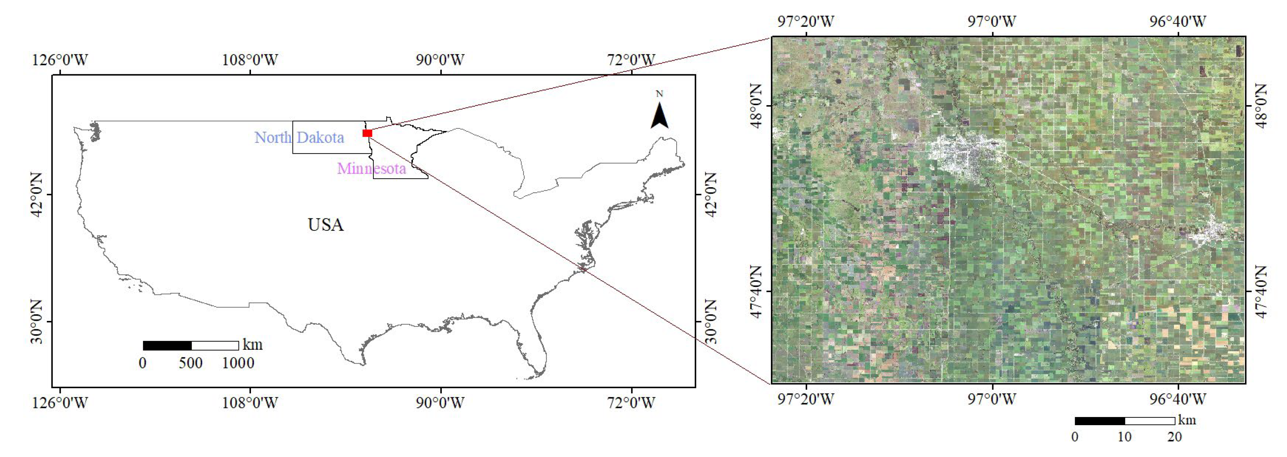
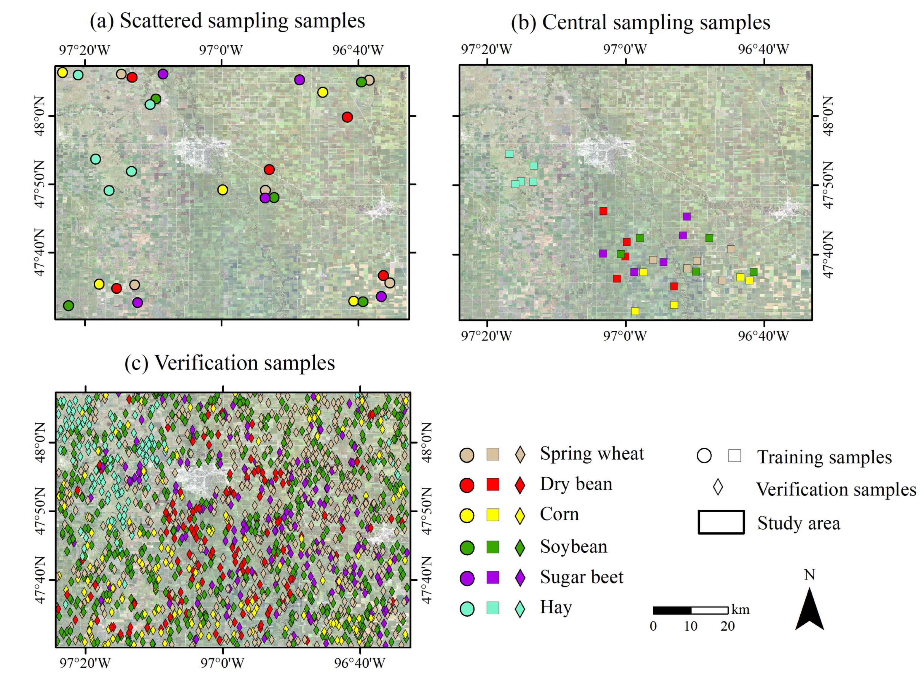
2.1. Study Area
2.2. Data Sources
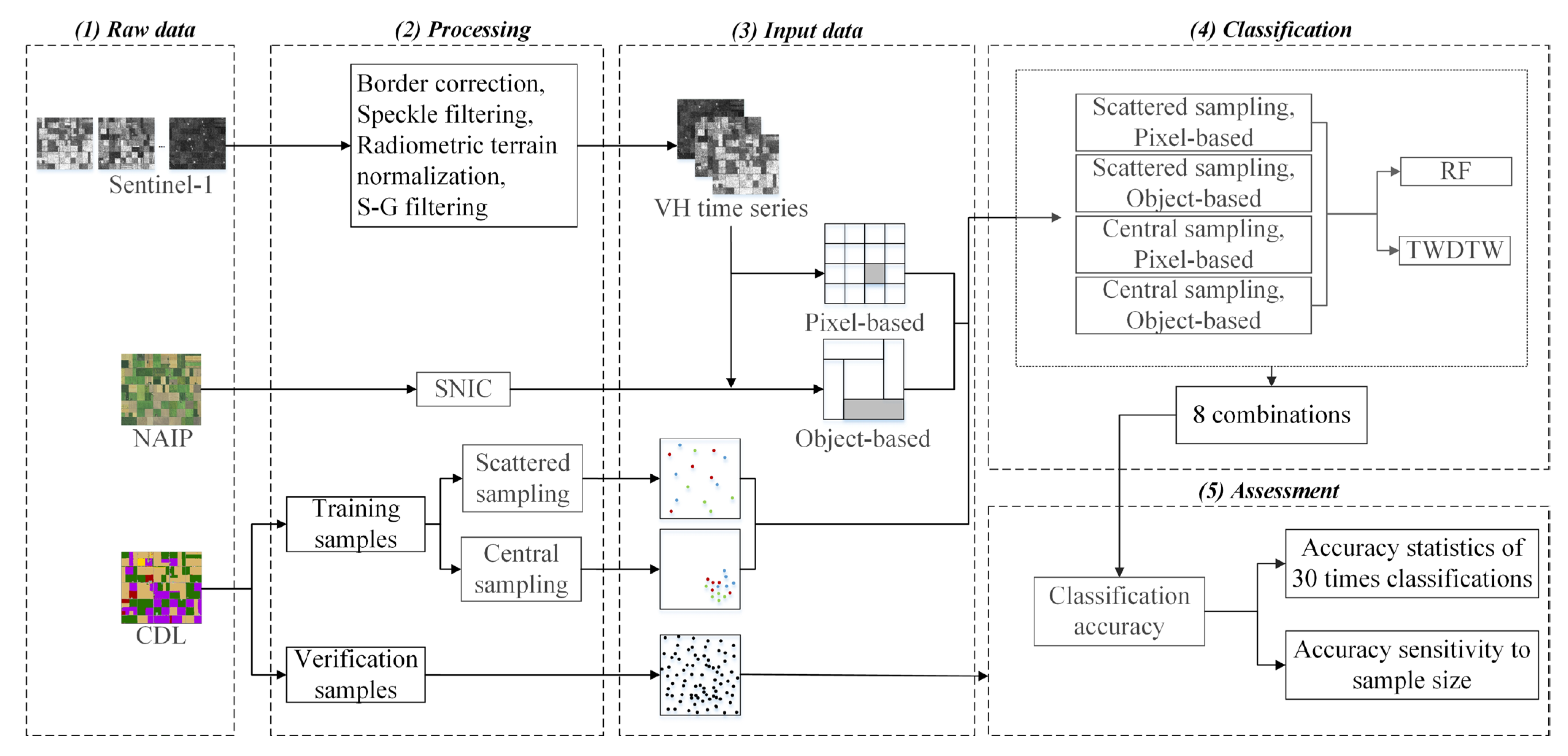
2.3. Methods
2.3.1. Simple Non-Iterative Clustering (SNIC) Image Segmentation
2.3.2. Time-Weighted Dynamic Time Warping (TWDTW)
2.3.3. Random Forest Classification
2.3.4. Classification Accuracy Assessment
2.3.5. Sensitivity Assessment of Classification Accuracy to Sample Size
3. Results
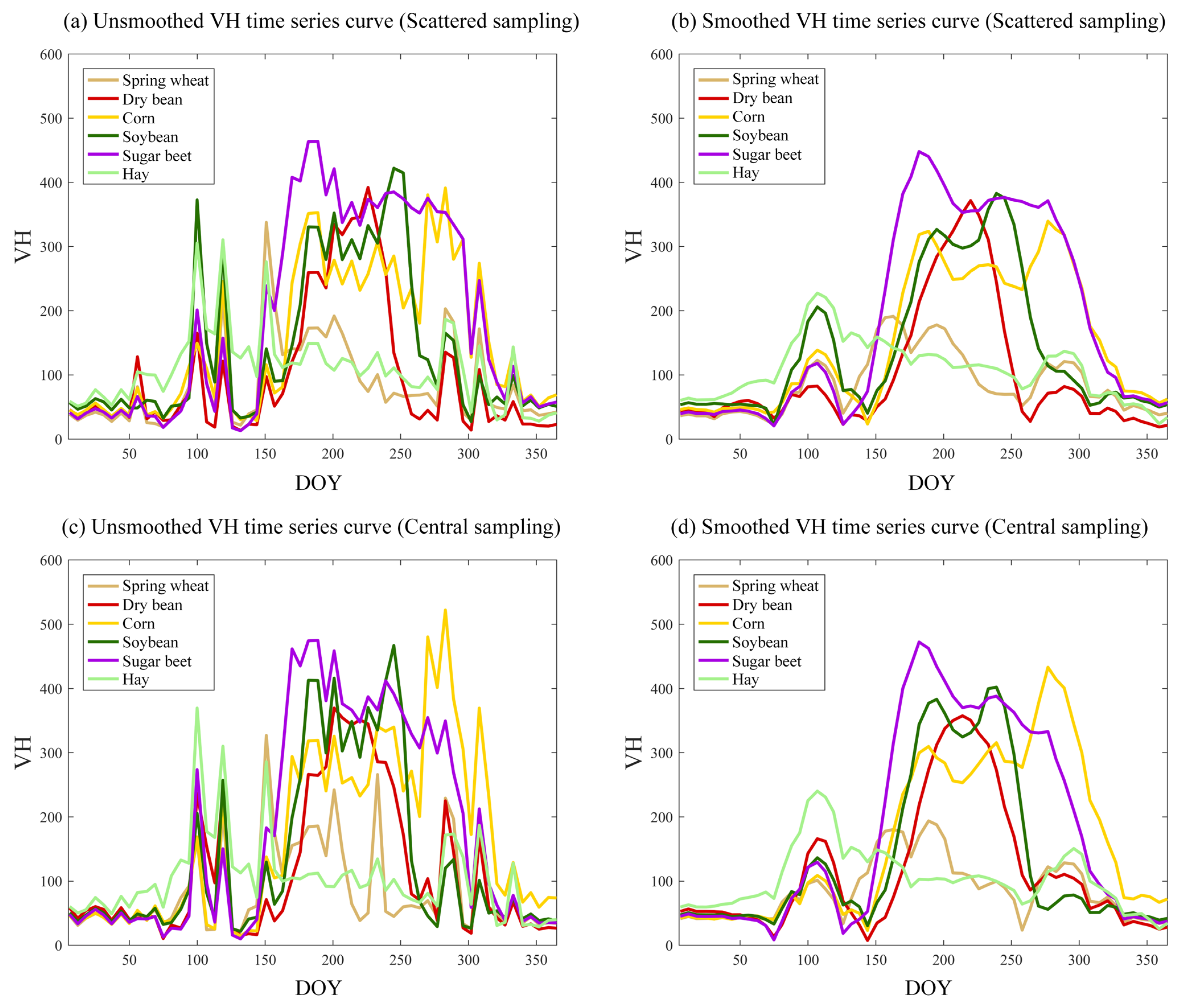
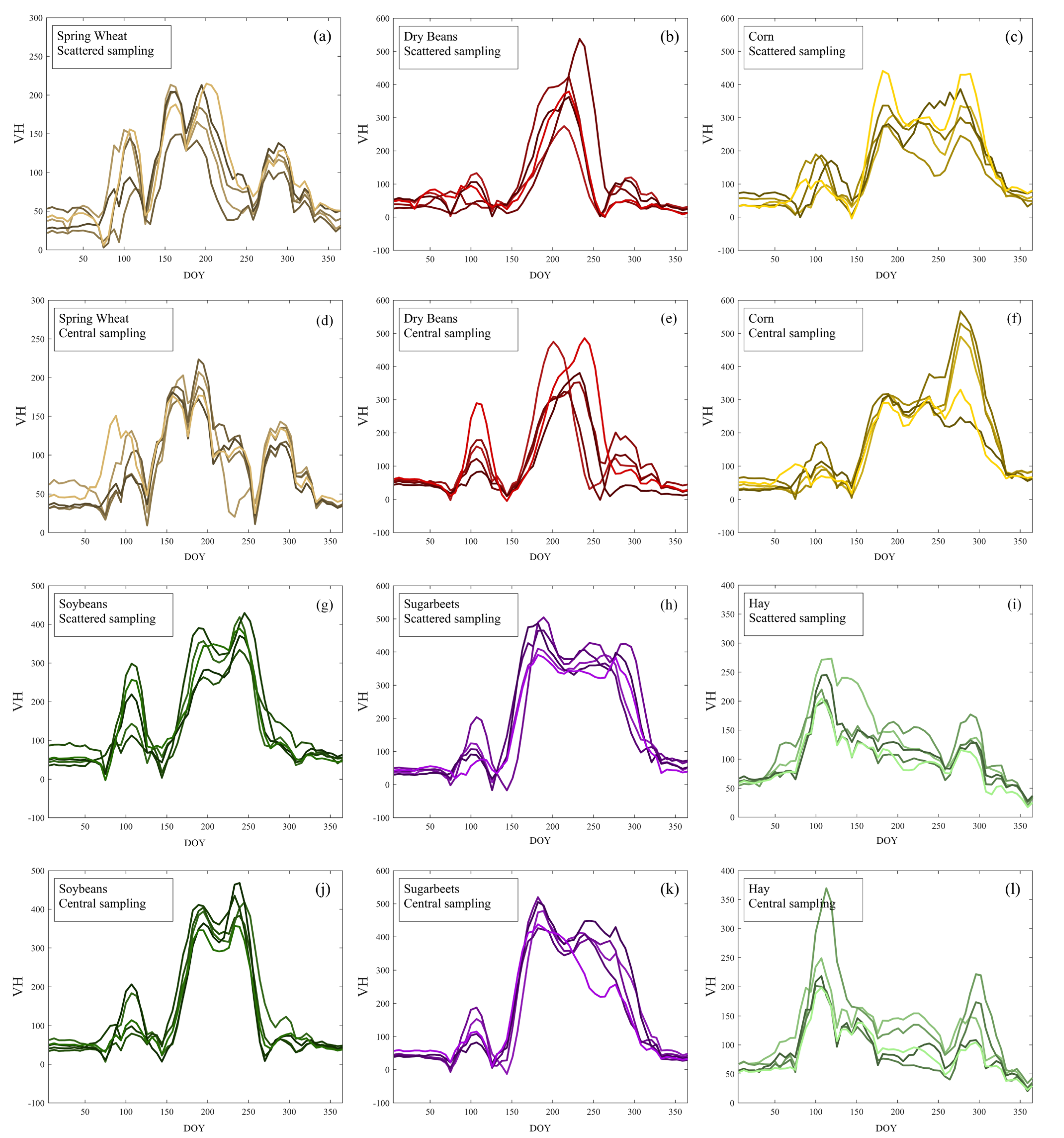
3.1. Time Series Curves of Major Crop Types
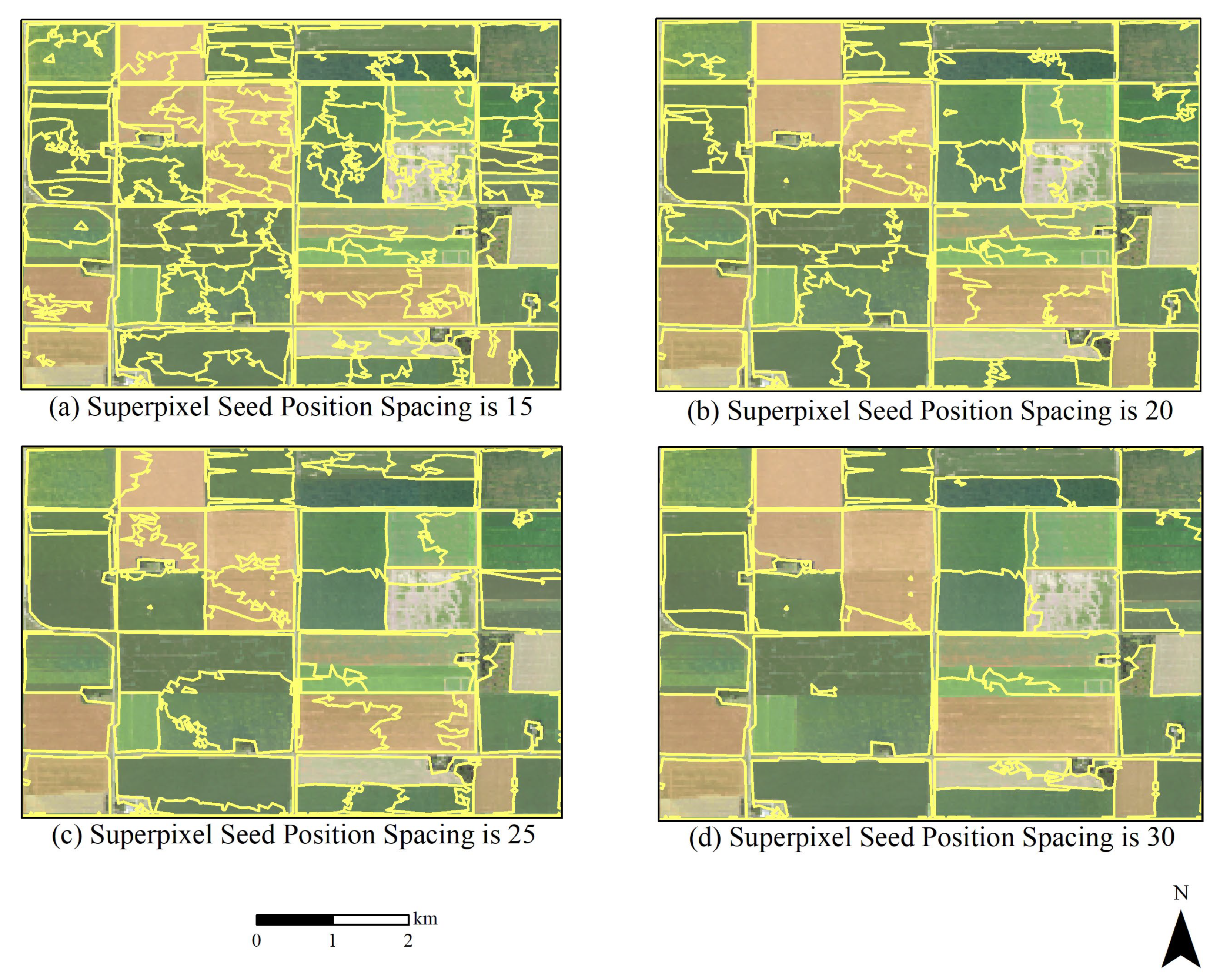
3.2. SNIC Image Segmentation Results
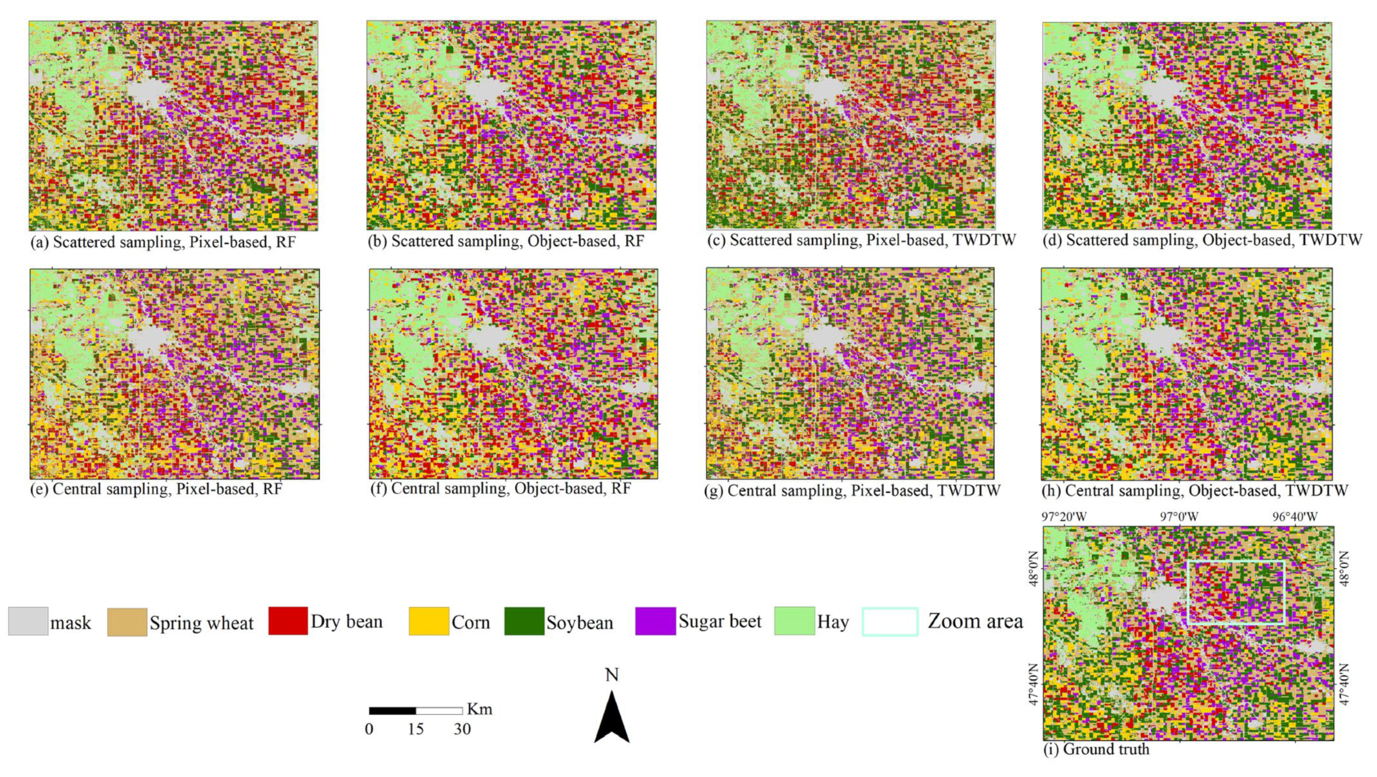
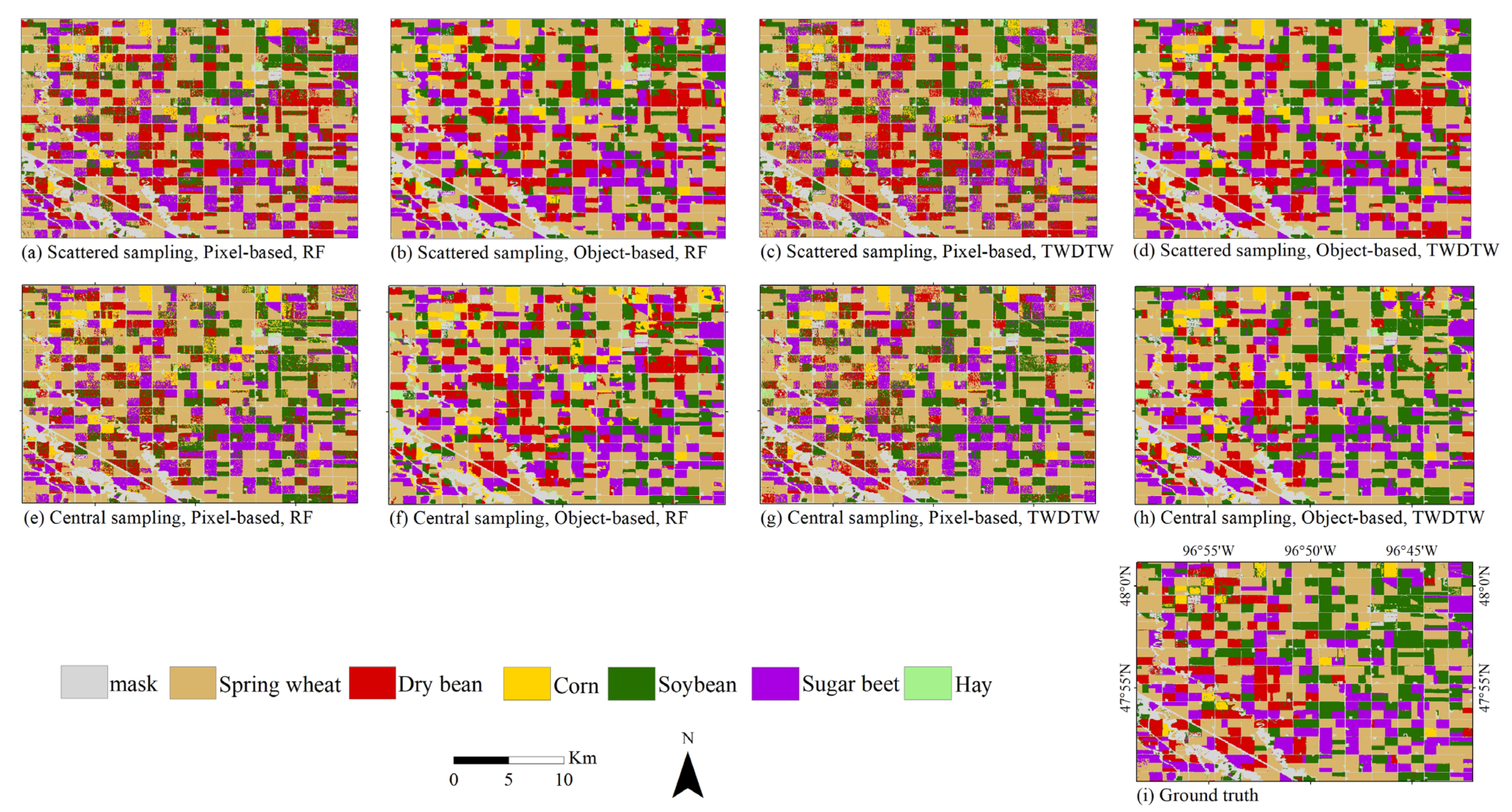
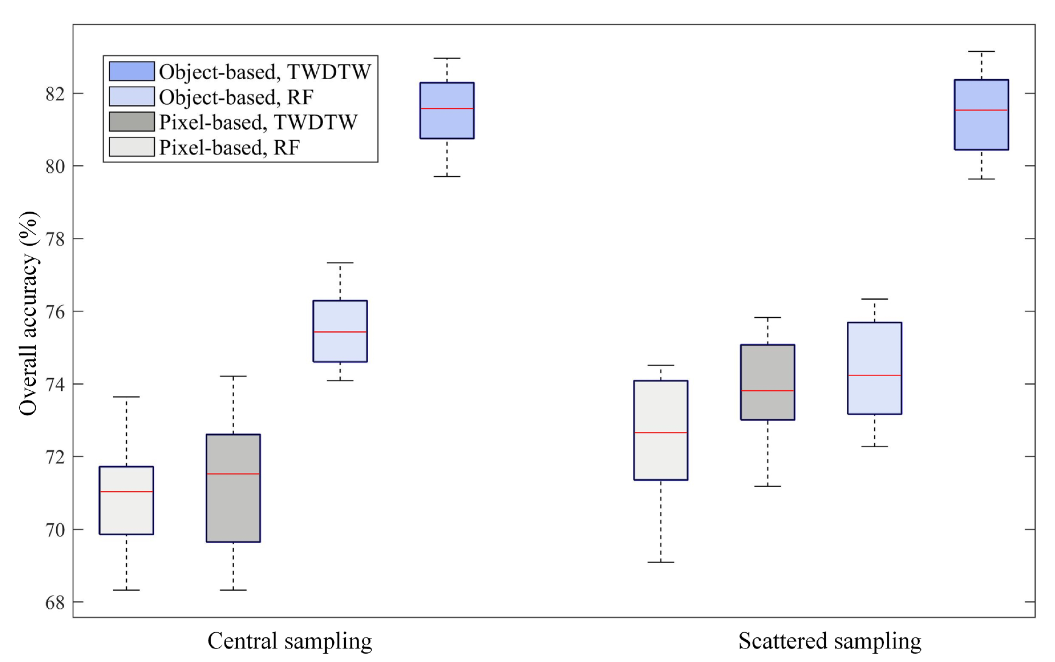
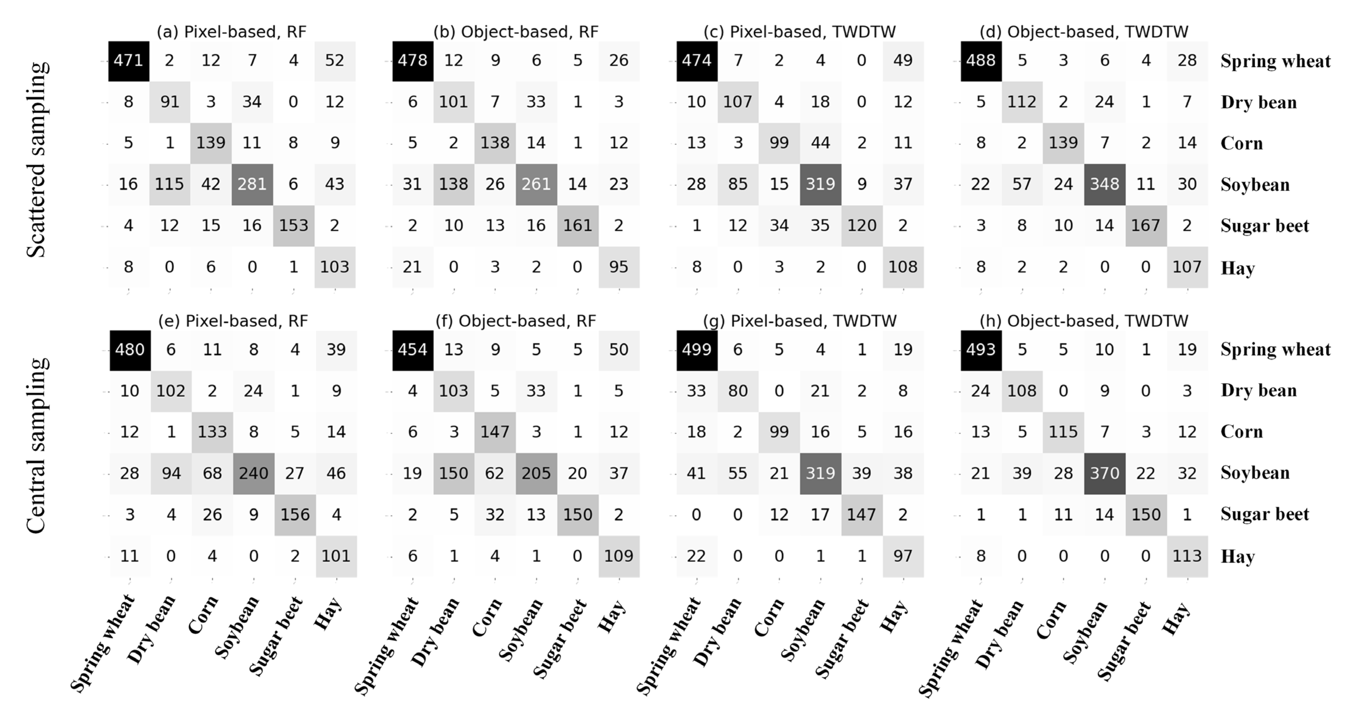
3.3. Comparisons of Different Classification Results and Accuracies
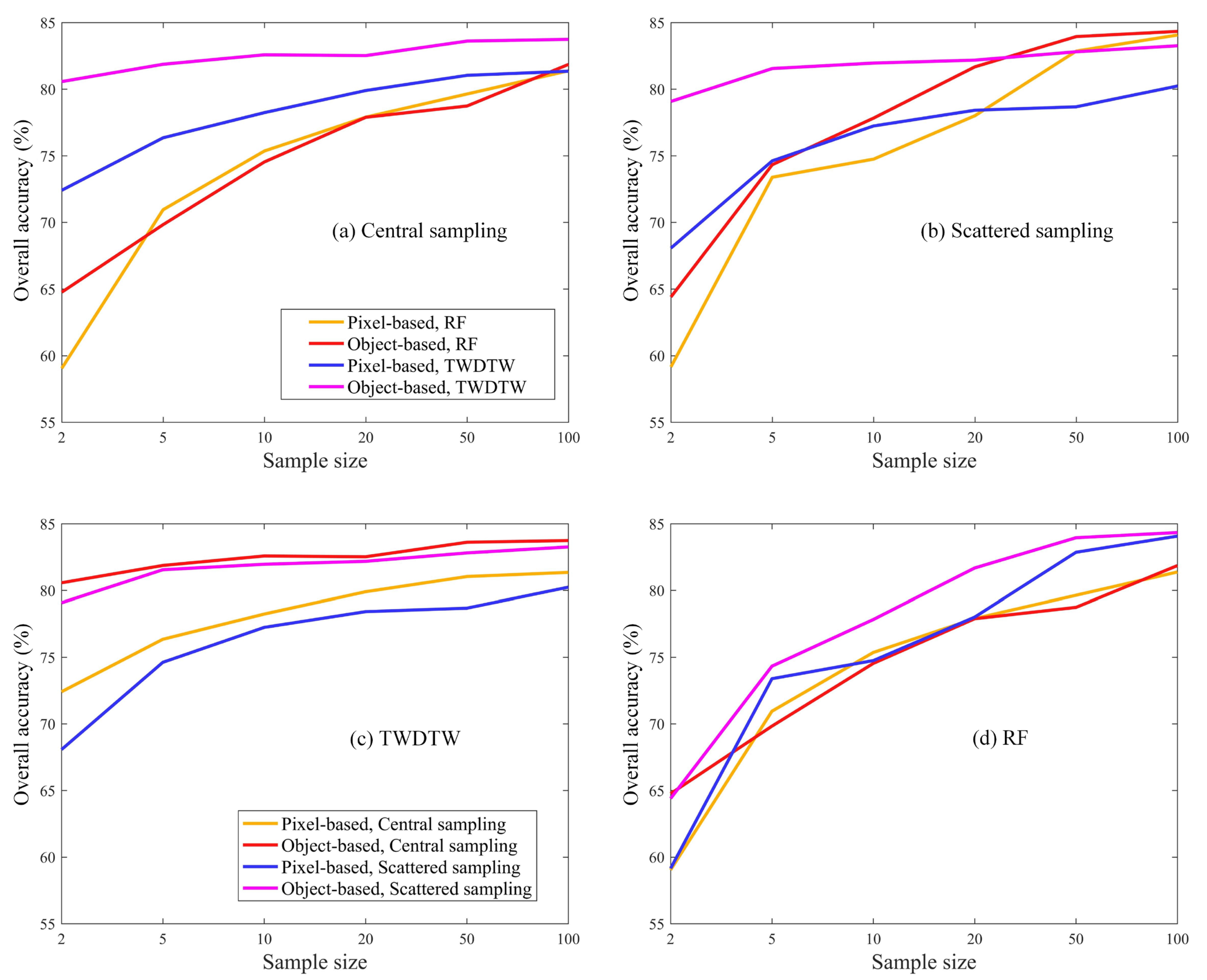
3.4. Sensitivities of Different Classification Strategies to Sample Size
4. Discussion
4.1. Advantages of GEE Platform and Sentinel-1 SAR Images for Crop Classification
4.2. Implications for Crop Classification and Sustainable Agricultural Management
4.3. Limitations and Future Research Topics
5. Conclusions
Author Contributions
Funding
Data Availability Statement
Acknowledgments
Conflicts of Interest
References
- Liu, Y.; Song, W. Modelling crop yield, water consumption, and water use efficiency for sustainable agroecosystem management. J. Clean. Prod. 2020, 253, 119940. [Google Scholar] [CrossRef]
- Godfray, H.C.J.; Beddington, J.R.; Crute, I.R.; Haddad, L.; Lawrence, D.; Muir, J.F.; Pretty, J.; Robinson, S.; Thomas, S.M.; Toulmin, C. Food security: The challenge of feeding 9 billion people. Science 2010, 327, 812–818. [Google Scholar] [CrossRef] [PubMed] [Green Version]
- Brown, M.; De Beurs, K.; Marshall, M. Global phenological response to climate change in crop areas using satellite remote sensing of vegetation, humidity and temperature over 26 years. Remote Sens. Environ. 2012, 126, 174–183. [Google Scholar] [CrossRef]
- Liu, Y.; Song, W.; Deng, X. Spatiotemporal patterns of crop irrigation water requirements in the Heihe River Basin, China. Water 2017, 9, 616. [Google Scholar] [CrossRef] [Green Version]
- Liu, Y.; Song, W.; Mu, F. Changes in ecosystem services associated with planting structures of cropland: A case study in Minle County in China. Phys. Chem. Earth Parts A/B/C 2017, 102, 10–20. [Google Scholar] [CrossRef]
- Li, H.; Zhang, C.; Zhang, S.; Atkinson, P.M. Full year crop monitoring and separability assessment with fully-polarimetric L-band UAVSAR: A case study in the Sacramento Valley, California. Int. J. Appl. Earth Obs. Geoinf. 2019, 74, 45–56. [Google Scholar] [CrossRef] [Green Version]
- Xiao, X.; Li, X.; Jiang, T.; Tan, M.; Hu, M.; Liu, Y.; Zeng, W. Response of net primary production to land use and climate changes in the middle-reaches of the Heihe River Basin. Ecol. Evol. 2019, 9, 4651–4666. [Google Scholar] [CrossRef] [Green Version]
- Csillik, O.; Belgiu, M.; Asner, G.P.; Kelly, M. Object-based time-constrained dynamic time warping classification of crops using Sentinel-2. Remote Sens. 2019, 11, 1257. [Google Scholar] [CrossRef] [Green Version]
- Liu, Y.; Song, W.; Deng, X. Changes in crop type distribution in Zhangye City of the Heihe River Basin, China. Appl. Geogr. 2016, 76, 22–36. [Google Scholar] [CrossRef]
- Gao, F.; Anderson, M.C.; Zhang, X.; Yang, Z.; Alfieri, J.G.; Kustas, W.P.; Mueller, R.; Johnson, D.M.; Prueger, J.H. Toward mapping crop progress at field scales through fusion of Landsat and MODIS imagery. Remote Sens. Environ. 2017, 188, 9–25. [Google Scholar] [CrossRef] [Green Version]
- Pinter, P.J., Jr.; Ritchie, J.C.; Hatfield, J.L.; Hart, G.F. The agricultural research service’s remote sensing program. Photogramm. Eng. Remote Sens. 2003, 69, 615–618. [Google Scholar] [CrossRef] [Green Version]
- Boryan, C.; Yang, Z.; Mueller, R.; Craig, M. Monitoring US agriculture: The US department of agriculture, national agricultural statistics service, cropland data layer program. Geocarto Int. 2011, 26, 341–358. [Google Scholar] [CrossRef]
- USDA-NASS. Usda-National Agricultural Statistics Service, Cropland Data Layer; USDA-NASS: Washington, DC, USA, 2016. [Google Scholar]
- Fisette, T.; Rollin, P.; Aly, Z.; Campbell, L.; Daneshfar, B.; Filyer, P.; Smith, A.; Davidson, A.; Shang, J.; Jarvis, I. AAFC annual crop inventory. In Proceedings of the 2013 Second International Conference on Agro-Geoinformatics (Agro-Geoinformatics), Fairfax, VA, USA, 12–16 August 2013; pp. 270–274. [Google Scholar]
- Sannier, C.; Gilliams, S.; Ham, F.; Fillol, E. Use of Satellite Image Derived Products for Early Warning and Monitoring of the Impact of Drought on Food Security in Africa. In Time-Sensitive Remote Sensing; Springer: Berlin/Heidelberg, Germany, 2015; pp. 183–198. [Google Scholar]
- Gao, H.; Wang, C.; Wang, G.; Fu, H.; Zhu, J. A novel crop classification method based on ppfSVM classifier with time-series alignment kernel from dual-polarization SAR datasets. Remote Sens. Environ. 2021, 264, 112628. [Google Scholar] [CrossRef]
- Kennedy, R.E.; Yang, Z.; Cohen, W.B. Detecting trends in forest disturbance and recovery using yearly Landsat time series: 1. LandTrendr—Temporal segmentation algorithms. Remote Sens. Environ. 2010, 114, 2897–2910. [Google Scholar] [CrossRef]
- Melaas, E.K.; Friedl, M.A.; Zhu, Z. Detecting interannual variation in deciduous broadleaf forest phenology using Landsat TM/ETM+ data. Remote Sens. Environ. 2013, 132, 176–185. [Google Scholar] [CrossRef]
- Gómez, C.; White, J.C.; Wulder, M.A. Optical remotely sensed time series data for land cover classification: A review. ISPRS J. Photogramm. Remote Sens. 2016, 116, 55–72. [Google Scholar] [CrossRef] [Green Version]
- Gorelick, N.; Hancher, M.; Dixon, M.; Ilyushchenko, S.; Thau, D.; Moore, R. Google Earth Engine: Planetary-scale geospatial analysis for everyone. Remote Sens. Environ. 2017, 202, 18–27. [Google Scholar] [CrossRef]
- Mutanga, O.; Kumar, L. Google earth engine applications. Remote Sens. 2019, 11, 591. [Google Scholar] [CrossRef] [Green Version]
- Jiao, X.; Kovacs, J.M.; Shang, J.; McNairn, H.; Walters, D.; Ma, B.; Geng, X. Object-oriented crop mapping and monitoring using multi-temporal polarimetric RADARSAT-2 data. J. Photogramm. Remote Sens. 2014, 96, 38–46. [Google Scholar] [CrossRef]
- Tassi, A.; Vizzari, M. Object-oriented lulc classification in google earth engine combining snic, glcm, and machine learning algorithms. Remote Sens. 2020, 12, 3776. [Google Scholar] [CrossRef]
- Dong, Q.; Chen, X.; Chen, J.; Zhang, C.; Liu, L.; Cao, X.; Zang, Y.; Zhu, X.; Cui, X. Mapping winter wheat in North China using Sentinel 2A/B data: A method based on phenology-time weighted dynamic time warping. Remote Sens. 2020, 12, 1274. [Google Scholar] [CrossRef] [Green Version]
- Chaves, M.E.; Alves, M.d.C.; Sáfadi, T.; de Oliveira, M.S.; Picoli, M.C.; Simoes, R.E.; Mataveli, G.A. Time-weighted dynamic time warping analysis for mapping interannual cropping practices changes in large-scale agro-industrial farms in Brazilian Cerrado. Sci. Remote Sens. 2021, 3, 100021. [Google Scholar] [CrossRef]
- Liu, Y.; Wang, J. Revealing Annual Crop Type Distribution and Spatiotemporal Changes in Northeast China Based on Google Earth Engine. Remote Sens. 2022, 14, 4056. [Google Scholar] [CrossRef]
- Wilson, B.T.; Knight, J.F.; McRoberts, R.E. Harmonic regression of Landsat time series for modeling attributes from national forest inventory data. ISPRS J. Photogramm. Remote Sens. 2018, 137, 29–46. [Google Scholar] [CrossRef]
- Chen, Y.; Cao, R.; Chen, J.; Liu, L.; Matsushita, B. A practical approach to reconstruct high-quality Landsat NDVI time-series data by gap filling and the Savitzky–Golay filter. ISPRS J. Photogramm. Remote Sens. 2021, 180, 174–190. [Google Scholar] [CrossRef]
- Wan, Y.; Zhang, R.; Pan, X.; Fan, C.; Dai, Y. Evaluation of the Significant Wave Height Data Quality for the Sentinel-3 Synthetic Aperture Radar Altimeter. Remote Sens. 2020, 12, 3107. [Google Scholar] [CrossRef]
- McNairn, H.; Shang, J. A review of multitemporal synthetic aperture radar (SAR) for crop monitoring. Multitemporal Remote Sens. 2016, 20, 317–340. [Google Scholar] [CrossRef]
- Li, M.; Bijker, W. Vegetable classification in Indonesia using Dynamic Time Warping of Sentinel-1A dual polarization SAR time series. Int. J. Appl. Earth Obs. Geoinf. 2019, 78, 268–280. [Google Scholar] [CrossRef]
- Nagraj, G.M.; Karegowda, A.G. Crop mapping using SAR imagery: An review. Int. J. Adv. Res. Comput. Sci. 2016, 7, 47–52. [Google Scholar]
- Salehi, B.; Daneshfar, B.; Davidson, A.M. Accurate crop-type classification using multi-temporal optical and multi-polarization SAR data in an object-based image analysis framework. Int. J. Remote Sens. 2017, 38, 4130–4155. [Google Scholar] [CrossRef]
- Wu, Q.; Zhong, R.; Zhao, W.; Fu, H.; Song, K. A comparison of pixel-based decision tree and object-based Support Vector Machine methods for land-cover classification based on aerial images and airborne lidar data. Int. J. Remote Sens. 2017, 38, 7176–7195. [Google Scholar] [CrossRef]
- Luo, C.; Qi, B.; Liu, H.; Guo, D.; Lu, L.; Fu, Q.; Shao, Y. Using time series Sentinel-1 images for object-oriented crop classification in Google earth engine. Remote Sens. 2021, 13, 561. [Google Scholar] [CrossRef]
- Achanta, R.; Susstrunk, S. Superpixels and polygons using simple non-iterative clustering. In Proceedings of the IEEE Conference on Computer Vision and Pattern Recognition, Honolulu, HI, USA, 21–26 July 2017; pp. 4651–4660. [Google Scholar]
- Mahdianpari, M.; Salehi, B.; Mohammadimanesh, F.; Brisco, B.; Homayouni, S.; Gill, E.; DeLancey, E.R.; Bourgeau-Chavez, L. Big data for a big country: The first generation of Canadian wetland inventory map at a spatial resolution of 10-m using Sentinel-1 and Sentinel-2 data on the Google Earth Engine cloud computing platform. Can. J. Remote Sens. 2020, 46, 15–33. [Google Scholar] [CrossRef]
- Belgiu, M.; Drăguţ, L. Random forest in remote sensing: A review of applications and future directions. ISPRS J. Photogramm. Remote Sens. 2016, 114, 24–31. [Google Scholar] [CrossRef]
- Asam, S.; Gessner, U.; Almengor González, R.; Wenzl, M.; Kriese, J.; Kuenzer, C. Mapping Crop Types of Germany by Combining Temporal Statistical Metrics of Sentinel-1 and Sentinel-2 Time Series with LPIS Data. Remote Sens. 2022, 14, 2981. [Google Scholar] [CrossRef]
- Sakoe, H.; Chiba, S. Dynamic programming algorithm optimization for spoken word recognition. IEEE Trans. Acoust. Speech Signal Process. 1978, 26, 43–49. [Google Scholar] [CrossRef] [Green Version]
- Berndt, D.J.; Clifford, J. Using dynamic time warping to find patterns in time series. In Proceedings of the 3rd International Conference on Knowledge Discovery and Data Mining, Seattle, WA, USA, 31 July–1 August 1994; pp. 359–370. [Google Scholar]
- Maus, V.; Câmara, G.; Appel, M.; Pebesma, E. dtwsat: Time-weighted dynamic time warping for satellite image time series analysis in r. J. Stat. Softw. 2019, 88, 1–31. [Google Scholar] [CrossRef] [Green Version]
- Cheng, K.; Wang, J. Forest-type classification using time-weighted dynamic time warping analysis in mountain areas: A case study in southern China. Forests 2019, 10, 1040. [Google Scholar] [CrossRef] [Green Version]
- Maus, V.; Câmara, G.; Cartaxo, R.; Sanchez, A.; Ramos, F.M.; De Queiroz, G.R. A time-weighted dynamic time warping method for land-use and land-cover mapping. IEEE J. Sel. Top. Appl. Earth Obs. Remote Sens. 2016, 9, 3729–3739. [Google Scholar] [CrossRef]
- Huete, A.; Didan, K.; Miura, T.; Rodriguez, E.P.; Gao, X.; Ferreira, L.G. Overview of the radiometric and biophysical performance of the MODIS vegetation indices. Remote Sens. Environ. 2002, 83, 195–213. [Google Scholar] [CrossRef]
- Belgiu, M.; Csillik, O. Sentinel-2 cropland mapping using pixel-based and object-based time-weighted dynamic time warping analysis. Remote Sens. Environ. 2018, 204, 509–523. [Google Scholar] [CrossRef]
- Hird, J.N.; DeLancey, E.R.; McDermid, G.J.; Kariyeva, J. Google Earth Engine, open-access satellite data, and machine learning in support of large-area probabilistic wetland mapping. Remote Sens. 2017, 9, 1315. [Google Scholar] [CrossRef] [Green Version]
- Stasolla, M.; Neyt, X. An Operational Tool for the Automatic Detection and Removal of Border Noise in Sentinel-1 GRD Products. Sensors 2018, 18, 3454. [Google Scholar] [CrossRef] [PubMed] [Green Version]
- Lee, J.-S. Digital image enhancement and noise filtering by use of local statistics. IEEE Trans. Pattern Anal. Mach. Intell. 1980, PAMI-2, 165–168. [Google Scholar] [CrossRef] [Green Version]
- Vollrath, A.; Mullissa, A.; Reiche, J. Angular-based radiometric slope correction for Sentinel-1 on google earth engine. Remote Sens. 2020, 12, 1867. [Google Scholar] [CrossRef]
- Mullissa, A.; Vollrath, A.; Odongo-Braun, C.; Slagter, B.; Balling, J.; Gou, Y.; Gorelick, N.; Reiche, J. Sentinel-1 SAR Backscatter Analysis Ready Data Preparation in Google Earth Engine. Remote Sens. 2021, 13, 1954. [Google Scholar] [CrossRef]
- Farr, T.G.; Rosen, P.A.; Caro, E.; Crippen, R.; Duren, R.; Hensley, S.; Kobrick, M.; Paller, M.; Rodriguez, E.; Roth, L. The shuttle radar topography mission. Rev. Geophys. 2007, 45, 1–33. [Google Scholar] [CrossRef] [Green Version]
- Paris, J.F. Radar backscattering properties of corn and soybeans at frequencies of 1.6, 4.75, and 13.3 Ghz. IEEE Trans. Geosci. Remote Sens. 1983, GE-21, 392–400. [Google Scholar] [CrossRef]
- McNairn, H.; Shang, J.; Jiao, X.; Champagne, C. The contribution of ALOS PALSAR multipolarization and polarimetric data to crop classification. IEEE Trans. Geosci. Remote Sens. 2009, 47, 3981–3992. [Google Scholar] [CrossRef] [Green Version]
- Press, W.H.; Teukolsky, S.A. Savitzky-Golay smoothing filters. Comput. Phys. 1990, 4, 669–672. [Google Scholar] [CrossRef]
- Maxwell, A.E.; Warner, T.A.; Vanderbilt, B.C.; Ramezan, C.A. Land cover classification and feature extraction from National Agriculture Imagery Program (NAIP) Orthoimagery: A review. Photogramm. Eng. Remote Sens. 2017, 83, 737–747. [Google Scholar] [CrossRef]
- Achanta, R.; Shaji, A.; Smith, K.; Lucchi, A.; Fua, P.; Süsstrunk, S. SLIC superpixels compared to state-of-the-art superpixel methods. IEEE Trans. Pattern Anal. Mach. Intell. 2012, 34, 2274–2282. [Google Scholar] [CrossRef] [Green Version]
- Petitjean, F.; Kurtz, C.; Passat, N.; Gançarski, P. Spatio-temporal reasoning for the classification of satellite image time series. Pattern Recognit. Lett. 2012, 33, 1805–1815. [Google Scholar] [CrossRef] [Green Version]
- Virnodkar, S.S.; Pachghare, V.K.; Patil, V.; Jha, S.K. Application of machine learning on remote sensing data for sugarcane crop classification: A review. ICT Anal. Appl. 2020, 2, 539–555. [Google Scholar] [CrossRef]
- Li, F.; Ren, J.; Wu, S.; Zhao, H.; Zhang, N. Comparison of regional winter wheat mapping results from different similarity measurement indicators of NDVI time series and their optimized thresholds. Remote Sens. 2021, 13, 1162. [Google Scholar] [CrossRef]
- Gella, G.W.; Bijker, W.; Belgiu, M. Mapping crop types in complex farming areas using SAR imagery with dynamic time warping. ISPRS J. Photogramm. Remote Sens. 2021, 175, 171–183. [Google Scholar] [CrossRef]
- Tatsumi, K.; Yamashiki, Y.; Torres, M.A.C.; Taipe, C.L.R. Crop classification of upland fields using Random forest of time-series Landsat 7 ETM+ data. Comput. Electron. Agric. 2015, 115, 171–179. [Google Scholar] [CrossRef]
- Hariharan, S.; Mandal, D.; Tirodkar, S.; Kumar, V.; Bhattacharya, A.; Lopez-Sanchez, J.M. A novel phenology based feature subset selection technique using random forest for multitemporal PolSAR crop classification. IEEE J. Sel. Top. Appl. Earth Obs. Remote Sens. 2018, 11, 4244–4258. [Google Scholar] [CrossRef] [Green Version]
- Saini, R.; Ghosh, S.K. Crop classification on single date sentinel-2 imagery using random forest and suppor vector machine. Int. Arch. Photogramm. Remote Sens. Spat. Inf. Sci. 2018, 42, 683–688. [Google Scholar] [CrossRef] [Green Version]
- Congalton, R.G. A review of assessing the accuracy of classifications of remotely sensed data. Remote Sens. Environ. 1991, 37, 35–46. [Google Scholar] [CrossRef]
- Lucieer, A.; Stein, A. Existential uncertainty of spatial objects segmented from satellite sensor imagery. IEEE Trans. Geosci. Remote Sens. 2002, 40, 2518–2521. [Google Scholar] [CrossRef] [Green Version]
- McGill, R.; Tukey, J.W.; Larsen, W.A. Variations of box plots. Am. Stat. 1978, 32, 12–16. [Google Scholar]
- Griffiths, P.; Nendel, C.; Hostert, P. Intra-annual reflectance composites from Sentinel-2 and Landsat for national-scale crop and land cover mapping. Remote Sens. Environ. 2019, 220, 135–151. [Google Scholar] [CrossRef]
- Kussul, N.; Lemoine, G.; Gallego, F.J.; Skakun, S.V.; Lavreniuk, M.; Shelestov, A.Y. Parcel-based crop classification in Ukraine using Landsat-8 data and Sentinel-1A data. IEEE J. Sel. Top. Appl. Earth Obs. Remote Sens. 2016, 9, 2500–2508. [Google Scholar] [CrossRef]
- Li, H.; Wan, J.; Liu, S.; Sheng, H.; Xu, M. Wetland Vegetation Classification through Multi-Dimensional Feature Time Series Remote Sensing Images Using Mahalanobis Distance-Based Dynamic Time Warping. Remote Sens. 2022, 14, 501. [Google Scholar] [CrossRef]
- Wang, X.; Hou, M.; Shi, S.; Hu, Z.; Yin, C.; Xu, L. Winter Wheat Extraction Using Time-Series Sentinel-2 Data Based on Enhanced TWDTW in Henan Province, China. Sustainability 2023, 15, 1490. [Google Scholar] [CrossRef]
- Huang, X.; Fu, Y.; Wang, J.; Dong, J.; Zheng, Y.; Pan, B.; Skakun, S.; Yuan, W. High-Resolution Mapping of Winter Cereals in Europe by Time Series Landsat and Sentinel Images for 2016–2020. Remote Sens. 2022, 14, 2120. [Google Scholar] [CrossRef]
- Zheng, Y.; Li, Z.; Pan, B.; Lin, S.; Dong, J.; Li, X.; Yuan, W. Development of a Phenology-Based Method for Identifying Sugarcane Plantation Areas in China Using High-Resolution Satellite Datasets. Remote Sens. 2022, 14, 1274. [Google Scholar] [CrossRef]
- Yuan, Y.; Wen, Q.; Zhao, X.; Liu, S.; Zhu, K.; Hu, B. Identifying Grassland Distribution in a Mountainous Region in Southwest China Using Multi-Source Remote Sensing Images. Remote Sens. 2022, 14, 1472. [Google Scholar] [CrossRef]
- Lv, S.; Xia, X.; Pan, Y. Optimization of Characteristic Phenological Periods for Winter Wheat Extraction Using Remote Sensing in Plateau Valley Agricultural Areas in Hualong, China. Remote Sens. 2023, 15, 28. [Google Scholar] [CrossRef]
- Logavitool, G.; Intarat, K.; Horanont, T. Integration of Machine Learning Algorithms and Time-Series Satellite Images on Land Use/Land Cover Mapping with Google Earth Engine. In Applied Geography and Geoinformatics for Sustainable Development, Proceedings of ICGGS 2022, Phuket, Thailand, 7–8 April 2022; Springer: Berlin/Heidelberg, Germany, 2022; pp. 171–182. [Google Scholar]
- Olivares, B.O.; Vega, A.; Calderón, M.A.R.; Rey, J.C.; Lobo, D.; Gómez, J.A.; Landa, B.B. Identification of Soil Properties Associated with the Incidence of Banana Wilt Using Supervised Methods. Plants 2022, 11, 2070. [Google Scholar] [CrossRef]
- Carr, T.; Mkuhlani, S.; Segnon, A.C.; Ali, Z.; Zougmoré, R.; Dangour, A.D.; Green, R.; Scheelbeek, P.F. Climate change impacts and adaptation strategies for crops in West Africa: A systematic review. Environ. Res. Lett. 2022, 17, 053001. [Google Scholar] [CrossRef]
- Vignola, R.; Esquivel, M.J.; Harvey, C.; Rapidel, B.; Bautista-Solis, P.; Alpizar, F.; Donatti, C.; Avelino, J. Ecosystem-Based Practices for Smallholders’ Adaptation to Climate Extremes: Evidence of Benefits and Knowledge Gaps in Latin America. Agronomy 2022, 12, 2535. [Google Scholar] [CrossRef]
- Harfenmeister, K.; Itzerott, S.; Weltzien, C.; Spengler, D. Agricultural monitoring using polarimetric decomposition parameters of sentinel-1 data. Remote Sens. 2021, 13, 575. [Google Scholar] [CrossRef]
- Hao, P.-Y.; Tang, H.-J.; Chen, Z.-X.; Meng, Q.-Y.; Kang, Y.-P. Early-season crop type mapping using 30-m reference time series. J. Integr. Agric. 2020, 19, 1897–1911. [Google Scholar] [CrossRef]


| Different Classification Methods | Overall Accuracy (%) | Kappa Coefficient | |
|---|---|---|---|
| Scattered sampling | Pixel-based, RF | 73.17 | 0.66 |
| Object-based, RF | 73.58 | 0.67 | |
| Pixel-based, TWDTW | 73.17 | 0.66 | |
| Object-based, TWDTW | 81.64 | 0.77 | |
| Central sampling | Pixel-based, RF | 71.63 | 0.64 |
| Object-based, RF | 69.65 | 0.62 | |
| Pixel-based, TWDTW | 75.39 | 0.68 | |
| Object-based, TWDTW | 82.11 | 0.77 | |
| Different Classification Methods | Spring Wheat | Dry Bean | Corn | Soybean | Sugar Beet | Hay | ||
|---|---|---|---|---|---|---|---|---|
| Scattered sampling | Pixel-based RF | User’s Accuracy Producer’s Accuracy | 92.0 85.9 | 41.2 61.5 | 64.1 80.3 | 80.5 55.9 | 89.0 75.7 | 46.6 87.3 |
| Object-based RF | User’s Accuracy Producer’s Accuracy | 88.0 89.2 | 38.4 66.9 | 70.4 80.2 | 78.6 52.9 | 88.5 78.9 | 59.0 78.5 | |
| Pixel-based TWDTW | User’s Accuracy Producer’s Accuracy | 88.7 88.1 | 50.0 70.9 | 63.1 57.6 | 75.6 64.7 | 91.6 58.8 | 48.9 89.3 | |
| Object-based TWDTW | User’s Accuracy Producer’s Accuracy | 91.9 91.6 | 59.5 74.8 | 76.7 79.7 | 87.8 70.7 | 90.3 82.4 | 56.0 92.4 | |
| Central sampling | Pixel-based RF | User’s Accuracy Producer’s Accuracy | 88.2 87.6 | 49.3 68.9 | 54.5 76.9 | 83.0 47.7 | 80.0 77.0 | 47.4 85.6 |
| Object-based RF | User’s Accuracy Producer’s Accuracy | 92.5 84.7 | 37.5 68.2 | 56.8 85.5 | 78.8 41.6 | 84.7 73.5 | 50.7 90.1 | |
| Pixel-based TWDTW | User’s Accuracy Producer’s Accuracy | 81.4 93.4 | 55.9 55.6 | 72.3 63.5 | 84.4 62.2 | 75.4 82.6 | 53.9 80.2 | |
| Object-based TWDTW | User’s Accuracy Producer’s Accuracy | 88.0 92.5 | 68.4 75.0 | 72.3 74.2 | 90.2 72.3 | 85.2 84.3 | 62.8 93.4 | |
Disclaimer/Publisher’s Note: The statements, opinions and data contained in all publications are solely those of the individual author(s) and contributor(s) and not of MDPI and/or the editor(s). MDPI and/or the editor(s) disclaim responsibility for any injury to people or property resulting from any ideas, methods, instructions or products referred to in the content. |
© 2023 by the authors. Licensee MDPI, Basel, Switzerland. This article is an open access article distributed under the terms and conditions of the Creative Commons Attribution (CC BY) license (https://creativecommons.org/licenses/by/4.0/).
Share and Cite
Xiao, X.; Jiang, L.; Liu, Y.; Ren, G. Limited-Samples-Based Crop Classification Using a Time-Weighted Dynamic Time Warping Method, Sentinel-1 Imagery, and Google Earth Engine. Remote Sens. 2023, 15, 1112. https://doi.org/10.3390/rs15041112
Xiao X, Jiang L, Liu Y, Ren G. Limited-Samples-Based Crop Classification Using a Time-Weighted Dynamic Time Warping Method, Sentinel-1 Imagery, and Google Earth Engine. Remote Sensing. 2023; 15(4):1112. https://doi.org/10.3390/rs15041112
Chicago/Turabian StyleXiao, Xingyuan, Linlong Jiang, Yaqun Liu, and Guozhen Ren. 2023. "Limited-Samples-Based Crop Classification Using a Time-Weighted Dynamic Time Warping Method, Sentinel-1 Imagery, and Google Earth Engine" Remote Sensing 15, no. 4: 1112. https://doi.org/10.3390/rs15041112