1. Introduction
An increasing number of electromagnetic disturbances possibly associated with earthquakes has been discovered by using satellite observations both in case studies and with statistical analyses [
1]. In this framework, a key problem is the cleaning and quality insurance of data in order to reduce spurious effects such as fluctuations of measurements not induced by the investigated events. For this purpose, an automatic procedure for electromagnetic field measurements will be particularly useful in terms of controlling artificial perturbations, as well as nonphysical background and electromagnetic noise. On the basis of CSES-01 measurements, Zhang et al. [
2] found a correlation between the variation in multiple parameters, such as electric field, recorded by CSES-01 and the location of the seismogenic region of a specific Indonesian earthquake. Marchetti et al. [
3] integrated CSES measurements (especially Ne) with those of other anomalies from the lithosphere and atmosphere, as well as Swarm satellite measurements, for large earthquakes in the Indonesian region. Liu et al. [
4] Liu evaluated the data quality of satellite measurements of ionospheric parameters by comparing them with in situ observations and ionosonde data. Yang et al. [
5] analyzed used satellite data from the China Seismo-Electromagnetic Satellite to analyze the geomagnetic polarization of 12 typical earthquakes from December 2018 to January 2023. Wang et al. [
6] investigated the electromagnetic effects of earthquakes and their potential impact on space weather through analysis of data from the CSES. Guo et al. [
7] focused on the seismo-ionospheric effects related to two earthquakes in Taiwan, which were detected by the China Seismo-Electromagnetic Satellite. The results suggested that earthquakes in Taiwan and the surrounding region may have affected the ionosphere through geochemical, acoustic, and electromagnetic channels.
In addition, data quality verification is an important part of studies on seismo-electromagnetic monitoring from space, and is key to the data management process in satellite missions. The main differentiating factor of geophysical investigations performed by satellite with respect to other ground measurements is that the same observation cannot be made in situ, and that the method of data quality verification is relatively more complex. Many authors have conducted in-depth studies on the extraction of features of electric fields possibly associated with earthquakes, and on the procedures for cleaning data of possible electromagnetic interferences using combinations of cutting-edge technologies. Some researchers have attempted the extraction of anomalous electromagnetic disturbances using techniques based on artificial intelligence, such as applying deep learning directly to time series, or to spectrograms, etc. Kanarachos et al. [
8] proposed a signal processing algorithm that combines wavelets, neural networks, and Hilbert transformation to detect anomalies in geoelectric field signals when investigating seismic precursors. Zeren et al. [
9] conducted the exploration of time-corrected cross-calibrating methods using three payloads (EFD, SCM and HPM) onboard a CSES-01. Yan et al. [
10] presented two types of regular features that were observed during LAP on board the CSES-01. The first feature is characterized by a sudden drop in plasma potential and floating potential data, while the second one manifests as a spike in the dayside plasma potential and floating potential data. Wang et al. [
11] employed data from five ionosonde stations and one incoherent scatter radar observatory to validate the radio occultation measurements obtained by the CSES satellite. Yuan et al. [
12] applied algorithms for the automatic recognition of lightning whistler acoustic waves on search-coil magnetometer (SCM) data from CSES-01; designed fuzzy and L morphology convolution kernels to identify the characteristics of spectral and L morphological features of whistlers; and used the SVM classifier to perform feature classification. Yan et al. [
13] demonstrated the reliability of in situ plasma parameters derived from the China Seismo-Electromagnetic Satellite. Chen et al. [
14] showed that CSES-01 Ne data very effectively reflect solar activity, as the trend in the former is highly correlated with the trend of variations in sunspot numbers. Liu et al. [
15] investigated potential seismic anomalies related to the Luding Ms6.8 earthquake that occurred on 5 September 2022 by analyzing ionospheric, infrared radiation, atmospheric electrostatic field, and hot spring ion data, the results suggested that the observed multi-sphere coupling anomalies were associated with the occurrence of the earthquake. Diego et al. [
16] proposed a direct quantitative validation method based on CSES measurements of plasma parameters and the geomagnetic field. Zhao et al. [
17] established the seismogenic mechanism of ELF electromagnetic waves emitted by earthquakes, using ground-based and satellite observations. Yan et al. [
18] analyzed the correlation between electron Ne and Te in the topside ionosphere, utilizing in situ measurements obtained from four satellites (CSES-01, Swarm A and B and CHAMP).
The data gathered by CSES-01 are widely used, and the electric field data are full of information, including not only possible earthquake precursors but also indications of other disturbances of the near-Earth electromagnetic environment. Yang et al. [
19] developed a complete geomagnetic model for equatorial regions using CSES-01 data, which provided valuable insights into the Earth’s magnetic field in these areas. In another study, Ghamry et al. [
20] reported the first detection of Pi2 pulsation using CSES-01, which has implications for understanding plasma wave propagation in the Earth’s magnetosphere. Furthermore, Gou et al. [
21] carried out an examination of plasma bubbles using the multiparametric payloads of CSES, which revealed new information about their formation and dynamics. Marchetti et al. [
22] explored the effects of volcanic eruptions on the ionosphere using CSES-01 data, shedding light on the complex interactions between the Earth’s atmosphere and its magnetic field. In addition to these examples, Spogli et al. [
23] investigated geomagnetic storms using CSES-01 data, contributing to our understanding of space weather phenomena and their impact on Earth’s magnetic environment. Compared with classical machine learning algorithms, deep learning achieves higher recognition accuracy and a greater generalization ability. Among them, convolutional neural networks (CNNs) and recurrent neural networks (RNNs) are the two most commonly used and relevant [
24]. CNN is a deep learning neural network, simulating the learning mechanism of the human brain in order to ensure high accuracy of training samples and test samples, improve the efficiency of image labeling, and facilitate the management and updating of the image classification system. Therefore, in the present work, a CNN is proposed to identify and classify the steps that appear in waveform data of the electric field measured by the EFD payload of the CSES-01 in order to improve the quality of the data and increase the applicability of electric field measurements, thus providing reliable observations for further analyses including those studying seismo-electromagnetic emissions.
2. Overview of EFD
On 2 February 2018, CSES-01 was launched successfully. Its main objectives are to monitor the near-Earth space environment and to investigate possible EM perturbations. The satellite undertakes a circular Sun-synchronous orbit at an altitude of approximately 500 km, LTDN at 14:00, with a designed lifetime of 5 years [
25].
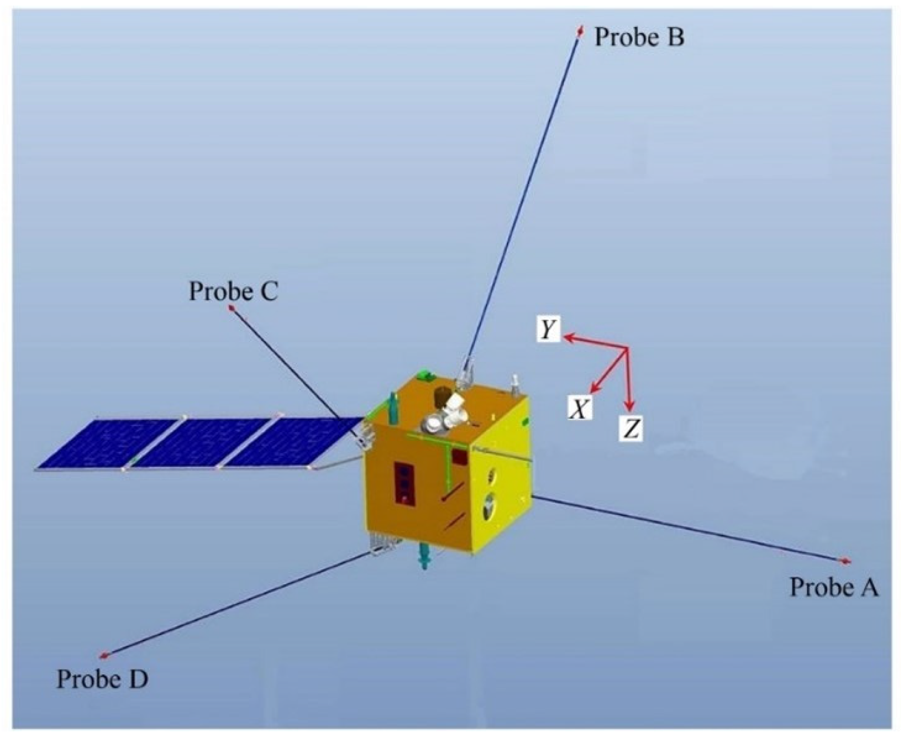
The Electric Field Detector (EFD) is designed for the measuring electric field in the space plasma environment, and is one of the main payloads of CSES-01. EFD adopts the active double-probe detection principle and is conceived for worldwide coverage, thus providing accurate and complete monitoring when studying electromagnetic perturbations possibly associated with the occurrence of earthquakes [
26]. The electric field is calculated from the difference in measured potential between two EFD probes. The EFD instrument is composed of four deployable booms, each of them carrying on their tip a 60 mm-diameter spherical probe (labeled “A”, “B”, “C”, and “D”, respectively) forming a tetrahedral structure. The {
X,
Y, and
Z} satellite coordinates system is defined as follows: the
X axis is parallel to the velocity vector of the satellite,
Z points in the direction of the nadir, and
Y points towards the point of intersection of
Z and
Y [
27], as shown in
Figure 1.
The intensity of the electric field vector is obtained by measuring—for each of the four probes—the difference of electric potential between the surface of a probe and the circuit ground, calculating the three differences of electric potential (dop) between pairs of the four probes and then dividing the dop between couples of probes for the distance between them. The EFD is designed to measure the intensity of the electric field components in the broad frequency range from DC to 3.5 MHz, subdivided into 4 channels, which are frequency bands, named: ULF (DC–16 Hz), ELF (6 Hz–2.2 kHz), VLF (1.8 kHz–20 kHz) and HF (18 kHz–3.5 MHz). According to the different data sampling rates at ULF, ELF, VLF and HF, the working period (WP) normally lasts 247.808 s. It is equally divided into 121 sub-working periods, each one lasting 2.048 s. The first of the 121 sub-working periods is called the bias current-corrected period (BCP). The other 120 2.048 s sub-working periods are called sampling periods (SP), and each SP is divided equally into 50 sub-sampling periods (SSP) of 40.96 ms. The data products from DPU are different in each of the different frequency bands. For the ELF frequency band, the sampling rate is 5 kHz and the outputs are each probe’s voltage values [
27].
3. Convolutional Neural Network Model
Convolutional Neural Network is the one of most common and interesting multilayer architectures used in deep learning. Compared with traditional models, CNNs are suitable for extracting feature information from images and audio recordings with high accuracy in recognition and classification [
28,
29] for image classification, target detection and behavior recognition, semantic segmentation, etc. Specific applications often require networks with different structures such as AlexNet, LeNet, VGGNet and ResNet [
30,
31,
32,
33].
In a CNN, the convolutional layer is the layer one with the role of extracting various features from the input, increasing the dimensional features by enhancing the useful ones, and reducing the effect of noise. The process of convolution is implemented through a convolution kernel, also known as a filter, which represents a feature that can be computed by sliding it over the input image by means of a sliding window, multiplying the kernel elements by the elements in the input region, and integrating in order to obtain the features of the input data [
34,
35], as follows:
where
is the element of the
m-row,
n-column of the
i-layer whose elements are being convolved,
denotes the element of the row
m +
a, column
n +
b of the
i − 1 input layer, and
presents the weight of the
a-row,
b-column of the kernel.
A convolutional layer usually contains multiple kernels. By computing the input matrix with different kernels, different features of the input data can be extracted. To increase the representational power of the model, bias terms are usually also added after the convolutional computation and the results are fed into a nonlinear activation function
f for nonlinear mapping in order to extract the features
of the data, with the following equation:
where
is the bias term of the
i layer,
is the number of channels of the
i layer,
is the weight matrix of the
i layer of the
k channel, which is the convolution kernel, and
is the output matrix of the
i − 1 layer of the
k channel.
To improve the accuracy of image feature acquisition and learning, the number of layers of convolutional neural networks usually needs to be deepened. Generally, the pooling layer is placed after the convolutional layer to reduce the amount of data processing and retain feature information by dimensioning down the convolutional output results to improve the generalization ability of the model.
The fully-connected layer acts as a “classifier” in a CNN, integrating features from the convolutional and pooling outputs and outputting classification results through the output layer. In the image classification task, the fully connected layer determines the class of the image based on the features extracted from the previous convolutional layers and pooling layers. The fully connected layer reshapes and integrates the two-dimensional feature map to produce the final output results. As for the output layer, a logistic function or a normalized exponential function is used to activate and release the output predicted values.
4. Experiment Design
4.1. Dataset Selection and Pre-Processing
In this article, we analyze the waveform of an electric field in the ELF band. In order to study the steps occurring in the electric field data, we consider 50 samples of an SSP data packet together with 50 samples of the previous SSP to obtain the image of the plot to be analyzed with the CNN algorithm. There are two types of steps: a straight-down step (that is a sudden and sharp decrease) and a smooth or gradual step, as shown in
Figure 2.
In signal processing data analysis, it is often necessary to segment data into different sections. For two adjacent data packets, A and B, we can use the following mathematical definitions to determine the types of connection between them:
Let MA and MB be the mean values of data packets A and B, respectively, while SA and SB are their variances, and KA and KB are their respective slopes.
- (1)
If |MA − MB| > 3SA, then the type of step connection between A and B is “straight-down”.
- (2)
If |MA − MB| ≤ 3SA:
- (i)
If KA × KB > 0, then the type of step connection between A and B is “progressive”;
- (ii)
If KA × KB < 0, then the type of step connection between A and B is “straight-down”.
4.2. CNN-Based Method for Detecting Steps Anomalies
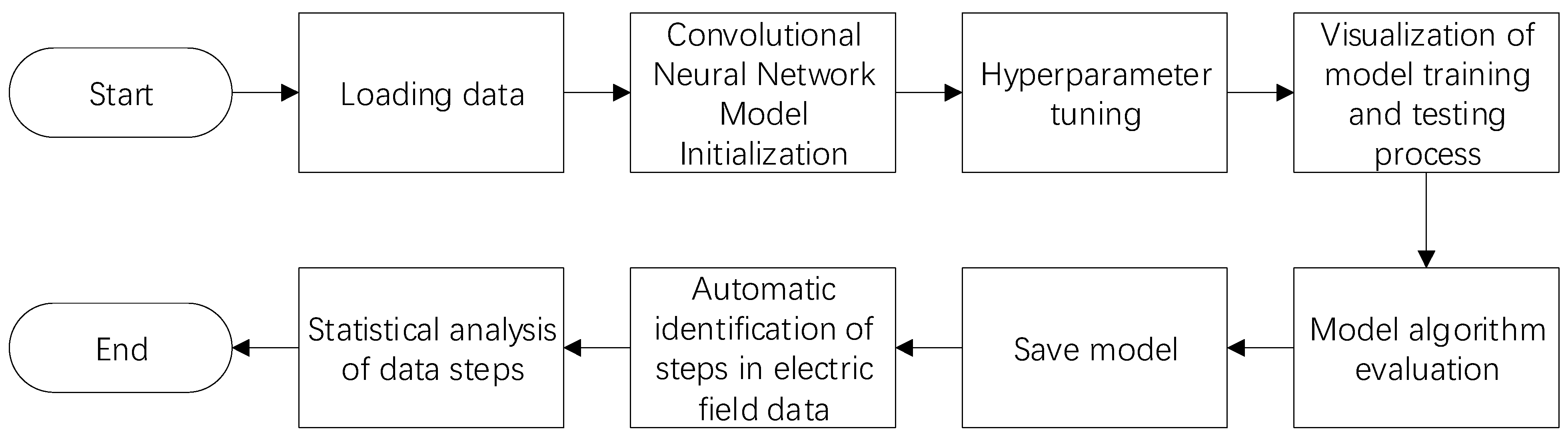
The flow chart of the recognition and classification algorithms for steps, based on CNN, is shown in
Figure 3. The main blocks of the process are the loading of the electric field waveform data; the initialization and hyperparameter tuning optimization of CNN; model training and testing visualization; algorithm evaluation; the automatic recognition of electric field steps, and statistical analysis.
The images fed to the CNN algorithm are plots of waveform obtained from the EFD experiment, which are divided into two categories: straight-down and progressive. Each class includes 1000 samples with 900 training images and 100 test images. These samples were manually screened and identified from the ELF band during the period of November 2019 to November 2020. Specifically, these samples include both straight-down and progressive types of data steps.
The training process of the CNN model is as follows:
- (1)
The fully connected layer of the model is applied to the dataset, and the output layer is replaced with a Softmax layer and an additional Dropout layer to avoid overfitting;
- (2)
Set appropriate values of hyperparameters according to the experimental conditions and dataset size. For example, set the value of batch_size to 32, the value of epoch to 50, and the value of initial learning rate to 0.001;
- (3)
Input the modified network model into the dataset and retrain it to get the new weights;
- (4)
Save the trained model and weights.
The testing process of the CNN model is as follows:
- (1)
Use the trained network model weights;
- (2)
Start the program to run the test sample through the CNN model layer by layer and output the results;
- (3)
Compare the output of the CNN model with the labels of the test samples, determine whether the output category of each image is correct, and perform statistics on the classification results;
- (4)
Repeat steps (2)~(3) until all images in the test set have been tested and classified.
In our study, we employed standard kernels with dimensions of 5 × 5 and 3 × 3. Specifically, we utilized 96 5 × 5 kernels in the initial and second layer, and finally incorporated 256 3 × 3 kernels in the third layer. To preserve the spatial resolution of the input images while extracting hierarchical features through convolutional layers, we employed zero-padding to ensure consistent spatial dimensions of the input and output feature maps throughout the network. This allowed us to maintain the original dimensions of the input images as they progressed through the network, while still enabling the extraction of increasingly abstract representations at each subsequent layer. In order to optimize the model, we utilized cross-validation during training to determine the optimal combination of hyperparameters. We calculated the average accuracy of the model on the test set and selected the hyperparameter combination that yielded the highest accuracy as the final training parameters for the model.
Table 1 shows the hyperparameters and optimization methods.
Due to the unbalanced number of samples in the categories of the dataset, which include many normal samples and few anomalous ones, the evaluation metrics of anomaly detection are generally more complex and cannot be calculated only for accuracy and loss values. The most commonly used evaluation index is the Receiver Operating Characteristic curve (ROC curve), which is more objective than accuracy and can characterize the results more comprehensively.
4.3. Analysis of Experimental Data
In training the CNN, the images in the dataset are first of all divided and labeled in categories. In the training process, images are used as input to the CNN for iterative training to shorten the training time. The accuracy and loss values of the training and test sets are shown in
Figure 4.
With the augmentation of iterations, there is a noticeable enhancement in the accuracy of both the training and test sets. With a number of iterations of approximately 50, the rate of improvement in the accuracy for both sets gradually stabilizes. When the training phase is complete, the accuracy of the model reaches 95.2% on the training set and 91.1% on the test set, while the value of the loss function is less than 0.1 on both training and test sets.
To verify the effectiveness of the developed classification algorithm, under different parameters, we have adopted the ROC curve to calculate the accuracy of each category. The abscissa of the ROC curve is False Positive Rate (FPR), and the ordinate is True Positive Rate (TPR), such that the ROC curve describes the equilibrium state of the classifier between TPR and FPR. The ROC curve has the important property that when the distribution of positive and negative samples in the test set changes, the ROC curve can remain unchanged, i.e., it is insensitive to the positive and negative sample imbalance problem. The closer the ROC curve is to the upper left corner, the better the performance of the classifier is. If the classifier’s performance is evaluated by the ROC curve, we can use the area under curve (AUC) metric, which is the area under the ROC curve, and takes values no more than 1. If a positive sample and a negative sample are randomly selected, the AUC characterizes the probability that these two samples are correctly distinguished. An example of ROC curve is shown in
Figure 5.
The ROC curves of
Figure 5 show that the CNN algorithm achieved high accuracy in the classification with AUC metrics higher than 90%. Therefore, the trained model can be applied to identify the steps of the electric field waveform in EFD data.
5. Experimental Results
CSES-01 adopts a near-circular Sun-synchronous orbit, and a complete orbit is divided into ascending (nighttime acquisition, at about 02:00 LT) and descending (daytime acquisition, at about 14:00 LT) semi-orbits for the satellite path from south to north latitudes, and vice versa. The CSES-01 revisit time is 5 days. In this article, we study the data of CSES-01 during a seismically quiet period. The orbit number ends with the digit 0 for descending and 1 for ascending, as per our analysis of the ELF waveform data collected from CSES-01.
To evaluate the performance of our model, we first analyzed four complete orbits during periods unaffected by external disturbances. Next, we extended our analysis to cover the revisit cycle of the CSES, which includes approximately 76 orbits, providing global-scale coverage. This allowed us to understand the regional characteristics of the data and further validate our model’s accuracy during these quiet periods. The results are presented in detail in
Section 5.1 and
Section 5.2.
5.1. Statistical Analysis of Steps in Ascending Semi-Orbits
The electric field data in the ELF band analyzed in this article are constituted by the waveforms of the three components (Ex, Ey, and Ez) evaluated on the basis of the differences of potential measured between the three pairs of probes ab, cd, and ad, respectively.
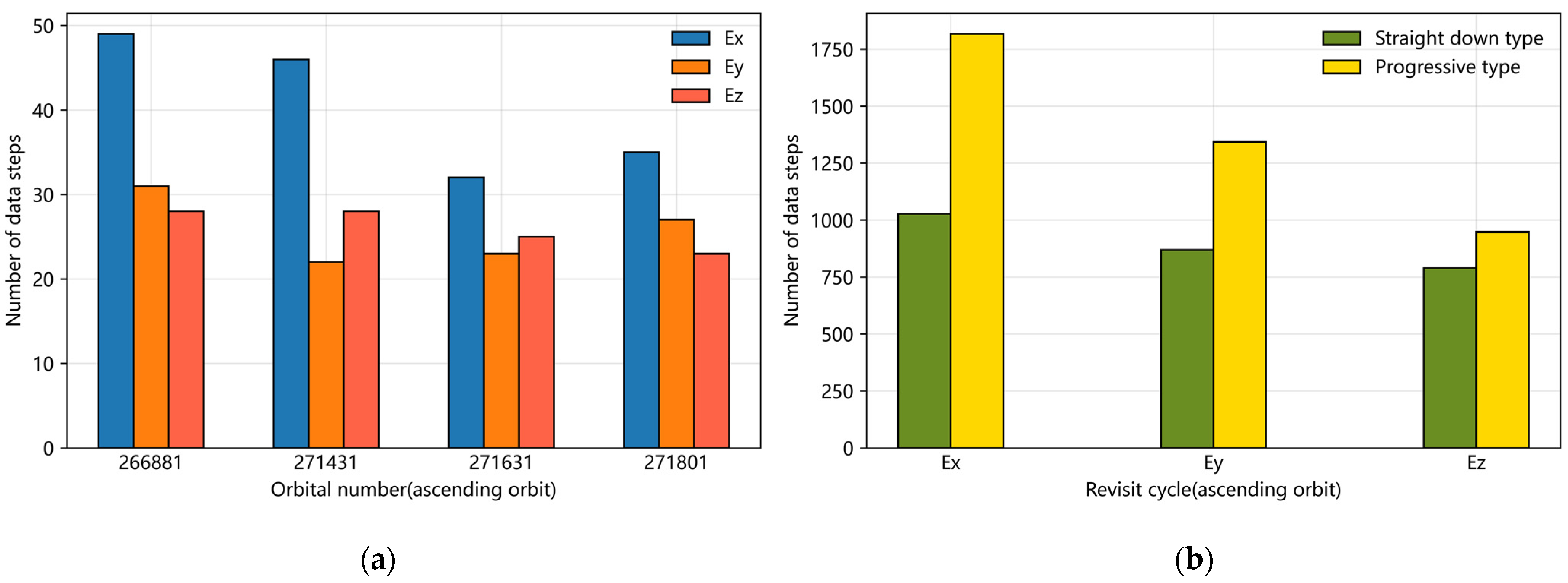
We selected the four ascending semi-orbits 26688, 27143, 27163, and 27180 in the period 16–20 December 2022 and conducted a further analysis on the ascending data within this revisit cycle. The results are shown in
Figure 6, where we provide the distribution of steps in each single semi-orbit (without distinguishing the step type) (
Figure 6a) and the distribution of straight-down and progressive steps for each electric field component, accumulated over the revisit cycle (
Figure 6b).
According to the statistical results shown in
Figure 6a, it can be found that the four selected ascending semi-orbits show similar distribution between the Ex, Ey, and Ez components, while
Figure 6b shows that in all components the number of progressive steps is higher than that of straight-down steps. However, there are some differences: in the 26688 orbit, the total number of both types of steps is 108 (with 25.93% of the straight-down type and 74.07% of the progressive type); in the 27143 orbit, the total number of both types of steps is 86 (with 39.53% of the straight-down type and 60.47% of the progressive type); in the 27163 orbit, the total number of both types of steps is 80 (with 45% of the straight-down type and 55% of the progressive type); finally, in the 27180 orbit, the total number of both types of steps is 86 (with 35.29% of the straight-down type and 64.71% of the progressive type).
Figure 6b shows that (i) the numbers of steps over Ex, Ey, and Ez components are similar, and (ii) the numbers of steps of both the straight-down and progressive types in the Ex component are higher than those in the Ey and Ez components. The total number of steps (of both types) in the ascending orbit of the revisit cycle is 6794, and the fraction of steps in the Ex component is 41.86%, in the Ey component it is 32.56%, and in the Ez component it is 25.58%.
5.2. Statistical Analysis of Steps in Descending Semi-Orbits
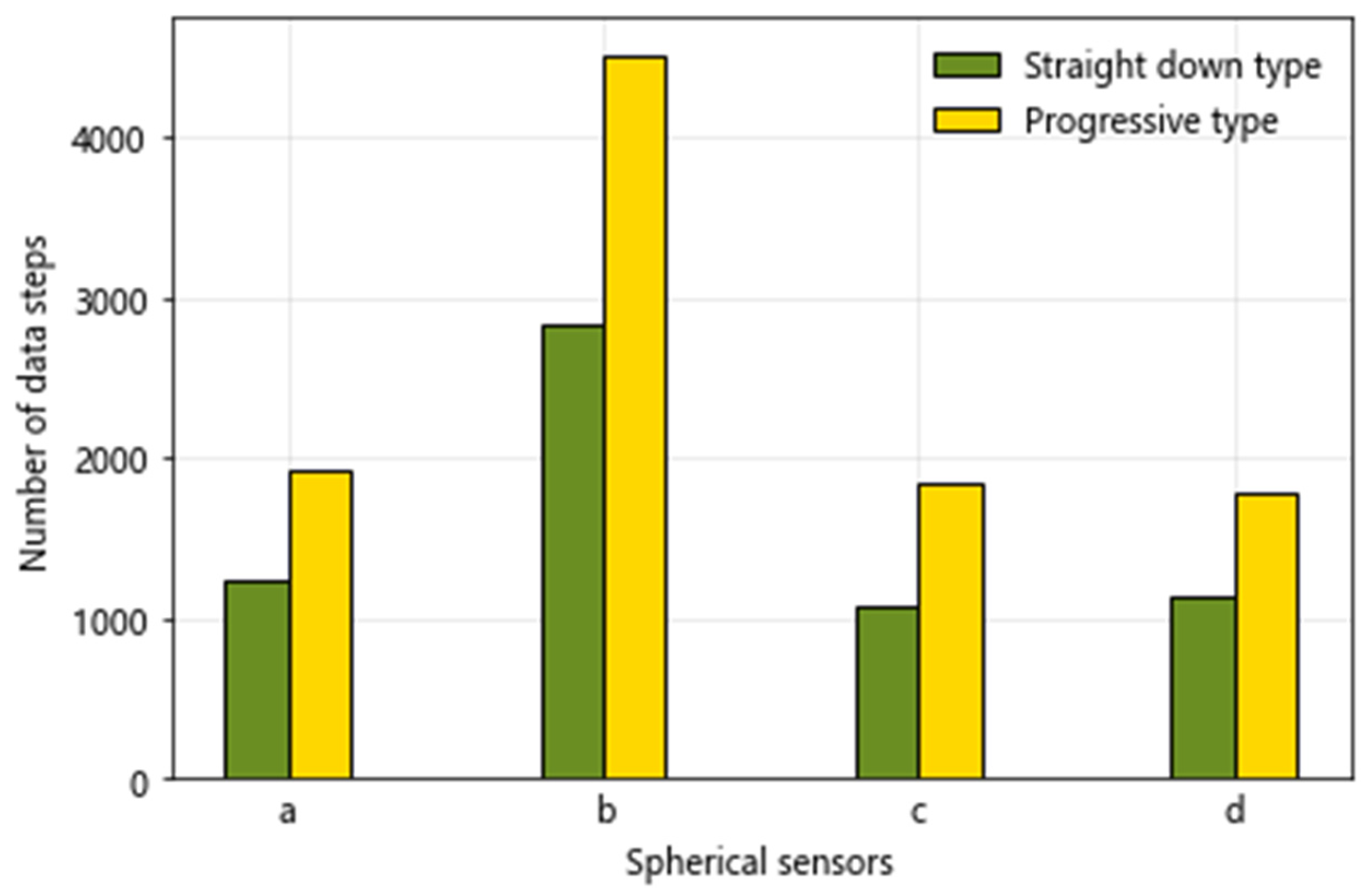
Based on the descending semi-orbits 26688, 27143, 27163, and 27180 in the period 16–20 December 2022, we conducted a further analysis on the descending data within this revisit cycle. The results are shown in
Figure 7, where we provide the distribution of steps in each single semi-orbit (without distinguishing the step type) (
Figure 7a) and the distribution of straight-down and progressive steps for each electric field component, accumulated over the revisit cycle of 16–20 December 2022 (
Figure 7b).
Figure 7a shows that, as in the ascending semi-orbits, in the descending ones, the number of steps shows a similar distribution in each of the Ex, Ey, and Ez components, and the number of steps in the Ex component is again the highest. In addition, the number of progressive steps is higher than that of straight-down ones, but there are some differences between different orbits. For example, in the 26688 orbit, the total number of the two types of steps is 156 (with 27.56% of the straight-down type and 72.44% of the progressive type); in the 27143 orbit, the total number of two types of steps is 128 (with 41.41% of the straight-down type and 58.59% of the progressive type); in the 27163 orbit, the total number of both types of steps is 157 (of which the percentage of straight-down type is 41.40%, while the percentage of progressive type is 58.60%); finally, in the 27180 orbit, the total number of both types of steps is 125 (of which the percentage of straight-down type is 42.40%, while the percentage of progressive type is 57.60%).
The statistical distribution of steps in descending semi-orbits is shown in
Figure 7b: the numbers of steps in the three components have similar distributions, with the Ex component showing the greatest difference between the numbers of the two step types and the highest absolute numbers of steps of both types with respect to the Ey and Ez components. The total number of steps of both types in the descending semi-orbits of the revisit cycle is 10,250, with 44.00% occurring in the Ex component, 31.20% in the Ey component, and 24.80% in the Ez component.
In summary, the number of step anomalies in the Ex component of the ELF electric field waveform is the highest. The statistical distributions of steps in different components show similar trends. These results need to be further explored to better understand the nature of this phenomenon. These findings are relevant to developing a deeper understanding of the operational state of the CSES-01 satellite, as well as of the data acquisition and data quality insurance processes.
7. Conclusions
This paper presents the first attempt at developing a method to automatically identify the occurrence of steps in electric field waveforms detected by EFD in ELF bands using CNN. Firstly, the EFD waveform data have been selected and pre-processed; secondly, the dataset is modeled and the model parameters are adjusted according to the test set results to obtain the best-performing model; finally, the data step anomalies are detected and identified automatically based on the model’s results. The experimental results show that, when using the CNN-based step anomaly detection algorithm, the accuracy and AUC index are higher than 90%.
The statistical analysis of the step anomalies in the waveform data shows that the most significant step anomalies are found in the Ex component. This study can provide an effective method for the automatic processing of waveform data and anomaly detection in an electric field. In order to avoid the influence of anomalous steps caused by seismic activity, by statistically analyzing the data steps during the quiet period, we find that the results of the data step analysis for individual tracks show consistency with those in the experimental part of this paper, further verifying the stability of the experimental results. Since the spherical sensor b—that is, the one most affected by step anomalies—is at the end of the boom in the direction of the satellite’s flight, and the step anomalies are more frequent in the Ex component waveform’s electric field component, we can hypothesize that the step anomaly is a trailing effect.
This study further demonstrates the importance of data quality assessment for increasing the effectiveness and optimizing the applicability of electric field data from EFD. However, it should be noted that the network model needs to be updated regularly according to the improvement of the classification system due to its relatively weak generalization ability. Meanwhile, it is also necessary to further explore how to improve the image recognition effect by refining the image sample design. The application of artificial intelligence methods to analyze EFD waveform data when detecting anomalies and classification problems has also been implemented, and this study provides support in exploring and applying artificial intelligence data analysis techniques in training algorithms for the identification and classification of typical phenomena. It also provides useful tools and methods for subsequent research on space electric field data derived via in earthquake monitoring from space environments.


 ,
, 


