Article

A Multi-Input Convolutional Neural Networks Model for Earthquake Precursor Detection Based on Ionospheric Total Electron Content

1
Electrical-Electronics Engineering Department, Engineering Faculty, Munzur University, Tunceli 62000, Turkey
2
Department of Geomatics Engineering, Kocaeli University, Kocaeli 41001, Turkey
3
Department of Electronics and Automation, Vocational School of Technical Sciences, Istanbul University-Cerrahpasa, Istanbul 34098, Turkey
4
Electrical-Electronics Engineering Department, Engineering Faculty, Bingol University, Bingol 12000, Turkey
5
Geological Engineering Department, Engineering Faculty, Firat University, Elazig 23119, Turkey
6
School of Geodesy and Geomatics, Wuhan University, 129 Luoyu Road, Wuhan 430079, China
7
Geomatics Engineering Department, Faculty of Engineering at Shoubra, Benha University, 108 Shoubra St., Cairo 11629, Egypt
8
Electrical-Electronics Engineering Department, Technology Faculty, Firat University, Elazig 23119, Turkey
*
Author to whom correspondence should be addressed.
Remote Sens. 2023, 15(24), 5690; https://doi.org/10.3390/rs15245690
Submission received: 11 November 2023 / Revised: 6 December 2023 / Accepted: 7 December 2023 / Published: 11 December 2023

Abstract

:
Earthquakes occur all around the world, causing varying degrees of damage and destruction. Earthquakes are by their very nature a sudden phenomenon and predicting them with a precise time range is difficult. Some phenomena may be indicators of physical conditions favorable for large earthquakes (e.g., the ionospheric Total Electron Content (TEC)). The TEC is an important parameter used to detect pre-earthquake changes by measuring ionospheric disturbances and space weather indices, such as the global geomagnetic index (Kp), the storm duration distribution (Dst), the sunspot number (R), the geomagnetic storm index (Ap-index), the solar wind speed (Vsw), and the solar activity index (F10.7), have also been used to detect pre-earthquake ionospheric changes. In this study, the feasibility of the 6th-day earthquake prediction by the deep neural network technique using the previous five consecutive days is investigated. For this purpose, a two-staged approach is developed. In the first stage, various preprocessing steps, namely TEC signal improvement and time-frequency representation-based TEC image construction, are performed. In the second stage, a multi-input convolutional neural network (CNN) model is designed and trained in an end-to-end fashion. This multi-input CNN model has a total of six inputs, and five of the inputs are designed as 2D and the sixth is a 1D vector. The 2D inputs to the multi-input CNN model are TEC images and the vector input is concatenated space weather indices. The network branches with the 2D inputs contain convolution, batch normalization, and Rectified Linear Unit (ReLU) activation layers, and the branch with the 1D input contains a ReLU activation layer. The ReLU activation outputs of all the branches are flattened and then concatenated. And the classification is performed via fully connected, softmax, and classification layers, respectively. In the experimental work, earthquakes with a magnitude of Mw5.0 and above that occurred in Turkey between 2012 and 2019 are used as the dataset. The TEC data were recorded by the Turkey National Permanent GNSS Network-Active (TNPGN-Active) Global Navigation Satellite System (GNSS) stations. The TEC data five days before the earthquake were marked as “precursor days” and the TEC data five days after the earthquake were marked as “normal days”. In total, 75% of the dataset is used to train the proposed method and 25% of the dataset is used for testing. The classification accuracy, sensitivity, specificity, and F1-score values are obtained for performance evaluations. The results are promising, and an 89.31% classification accuracy is obtained.

1. Introduction

The ionosphere is a layer of the Earth’s atmosphere that is a dispersive medium for electromagnetic signals. Accurate modeling of the number of free electrons in this layer has undeniable importance for satellite and communication systems since electromagnetic signals traveling between space and the Earth are affected by ionospheric plasma. This amount of electrons, which expresses the density of the plasma, is dominantly controlled by the sun. Ionosphere variation is also sensitive to natural and anthropogenic events, such as earthquakes, volcanoes, tsunamis, severe surface explosions, underground nuclear explosions, typhoons, and space weather [1,2,3,4,5,6,7,8,9]. This study focused on the interaction between earthquakes and the ionosphere.
The phenomenon of shaking of the environment and the Earth’s surface, in which the vibrations that occur suddenly due to fractures in the Earth’s crust spread out as waves, is called an “earthquake”. The plates that make up the Earth’s crust move slowly due to convective currents in the upper mantle, and they perform this movement along faults. Meanwhile, very violent ruptures and movements occur due to the friction and strain between the plates, causing earthquakes. Efforts to predict the time, magnitude, and location of an earthquake are very important in minimizing the loss of life and property caused by the event. The interaction between earthquakes and the ionosphere was first reported in the great 1964 Alaska earthquake [10]. In ongoing studies, some researchers have revealed the acoustic coupling processes from the lithosphere to the atmosphere for the 1968 Japan earthquake and the 1969 Kurile Islands earthquake [11,12]. In the late 1990s, it was discussed that seismo-ionosphere interaction could contribute to earthquake prediction [13,14]. In particular, the rapid development of Global Navigation Satellite System (GNSS) technology, which provides low-cost, high-accuracy, near-real-time, and continuous ionospheric data, has broadened the interest and scope of ionospheric precursor studies. The Total Electron Content (TEC) parameter is used to describe how many free electrons have been found in the ionosphere by GNSS measurements [15]. The amount of free electrons in a cylinder with a base area of 1 square meter along the GNSS signal line of sight is represented by the TEC.
There are many studies in the literature on ionospheric earthquake precursors using TEC data. In many of them, abnormal changes in the TEC variation, which are thought to be caused by earthquakes, were detected using classical anomaly detection methods [16,17,18,19,20,21,22,23,24,25,26,27,28,29,30]. About ten years ago, the first implementations of artificial intelligence (AI) techniques in earthquake–ionosphere studies were published in a series of articles [31,32,33,34]. The support vector machine (SVM), multi-layer perceptron, genetic algorithm, and adaptive network-based fuzzy inference system were utilized in these studies.
AI techniques can model future ionospheric variations with high accuracy, thus providing an advantage in anomaly detection in near real-time applications. In the last decade, the use of machine and deep learning techniques in ionospheric earthquake precursor studies has gained momentum to enable near real-time precursor detection [35,36,37,38,39,40,41,42,43,44,45,46,47,48,49,50,51,52,53,54,55,56]. Some researchers utilized an artificial neural network (ANN), particle swarm optimization, firefly algorithm, artificial bee colony, decision tree, bagging, and random forest methods to detect ionospheric and thermal anomalies before some strong earthquakes and compared the results with traditional anomaly detection methods [35,36,39,40,41]. Others proposed these new methods as a new predictive tool to detect seismo-ionospheric precursors because their results were quite promising. Several researchers [37,57,58] investigated the ability of the autoregressive integrated moving average (ARIMA) and long short-term memory (LSTM) network models to predict TEC time series and identify TEC anomalies. The results showed that both the ARIMA and LSTM methods can successfully detect ionospheric anomalies, but the performance of the LSTM is more robust compared to the ARIMA. In addition, the authors of [59] show that although local anomalies were observed at stations within Dobrovolsky’s earthquake preparation area (EPA), they were not observed at stations outside the EPA. In another study, an N-ANN (N-Model Neural Network Model) method was introduced for an AI-based early earthquake detection strategy [43]. The model was tested on 16 earthquake events in Sumatra and reached 76% accuracy. In [44], TEC data were trained with ANN for both magnitude classification and earthquake prediction. The ANN achieved an accuracy of 94.60% for magnitude classification and predicted the 2017 Mw 8.2 Mexico earthquake with an accuracy of 85.71%. A machine learning-based system for real-time earthquake prediction based on TEC data with geomagnetic indices was developed in [45]. The authors focused on 80 earthquakes greater than Mw 4.0 in Italy between 1 January 2014 and 30 September 2016 using SVM as a classifier. In total, 35 of these earthquakes were allocated as training, 21 as validation, and 24 as testing. In addition, 17 of the 21 earthquakes in the validation period and 22 of the 24 earthquakes in the test period were detected correctly. The authors of [38] used ionospheric TEC data that were derived from a GNSS network, and an SVM classifier to predict earthquake precursors 48 h in advance. The authors used 106 earthquake precursors that were greater than Mw 6.0 in their experiments and an 83% accuracy score was obtained. A system that uses the bidirectional LSTM (Bi-LSTM) network was proposed to estimate the TEC values of earthquakes of Mw 6.0 and above in Taiwan between 2003 and 2014 [50]. Along with the observed TEC values, they also tried to predict the TEC values by using some space weather indices that have an impact on the non-periodic changes of the TEC values, such as the Dst, F10.7, sunspot number, and solar emission index (Lyman–α). The authors labeled the TEC values before earthquakes of Mw 6.0 and above as the positive period (earthquake) and the TEC values before earthquakes of magnitude Mw 5.3 and above as the negative period (normal cases). As a result, 13 models were trained and 22/22 of positive cases and 10/19 of negative cases were predicted with an overall accuracy of 78.05%.
In this study, an artificial intelligence-based system was developed to distinguish the “precursor days” and “normal days” periods of ionospheric TEC variation associated with main shock earthquakes above Mw5.0, which have occurred in Turkey. The TEC time series were obtained based on daily satellite observations of 168 Global Navigation Satellite System (GNSS) stations belonging to the Turkey National Permanent GNSS Network-Active (TNPGN-Active). The TEC time series were converted to images in the time–frequency domain by continuous wavelet time–frequency transformation and used as input data together with six space weather indices (Vsw, Kp, R, Dst, Ap, and F10.7) to train an end-to-end trainable multi-input convolutional neural network (CNN) model, which is stronger than classical machine and deep learning networks. The main contributions of this paper are as follows:
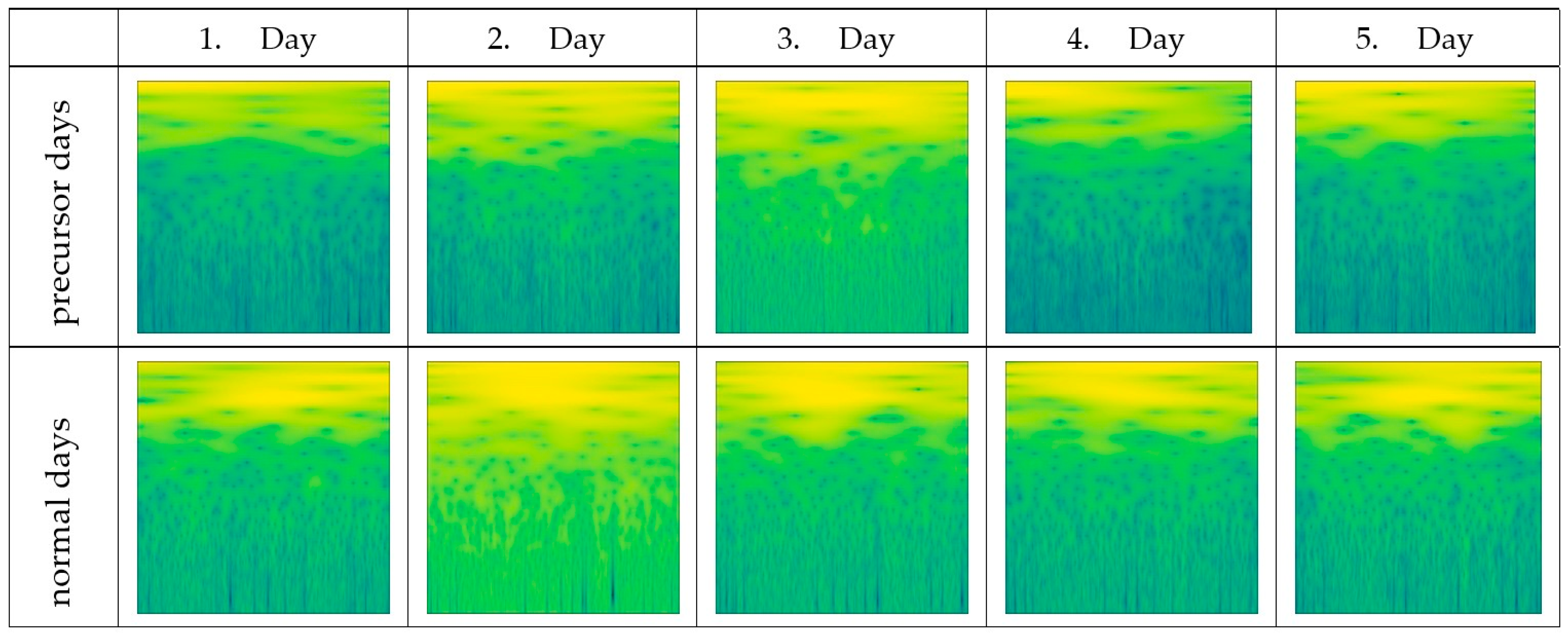
  • TEC time–frequency images are constructed and used as the input to a CNN model for “precursor days” and “normal days” prediction purposes for the first time.
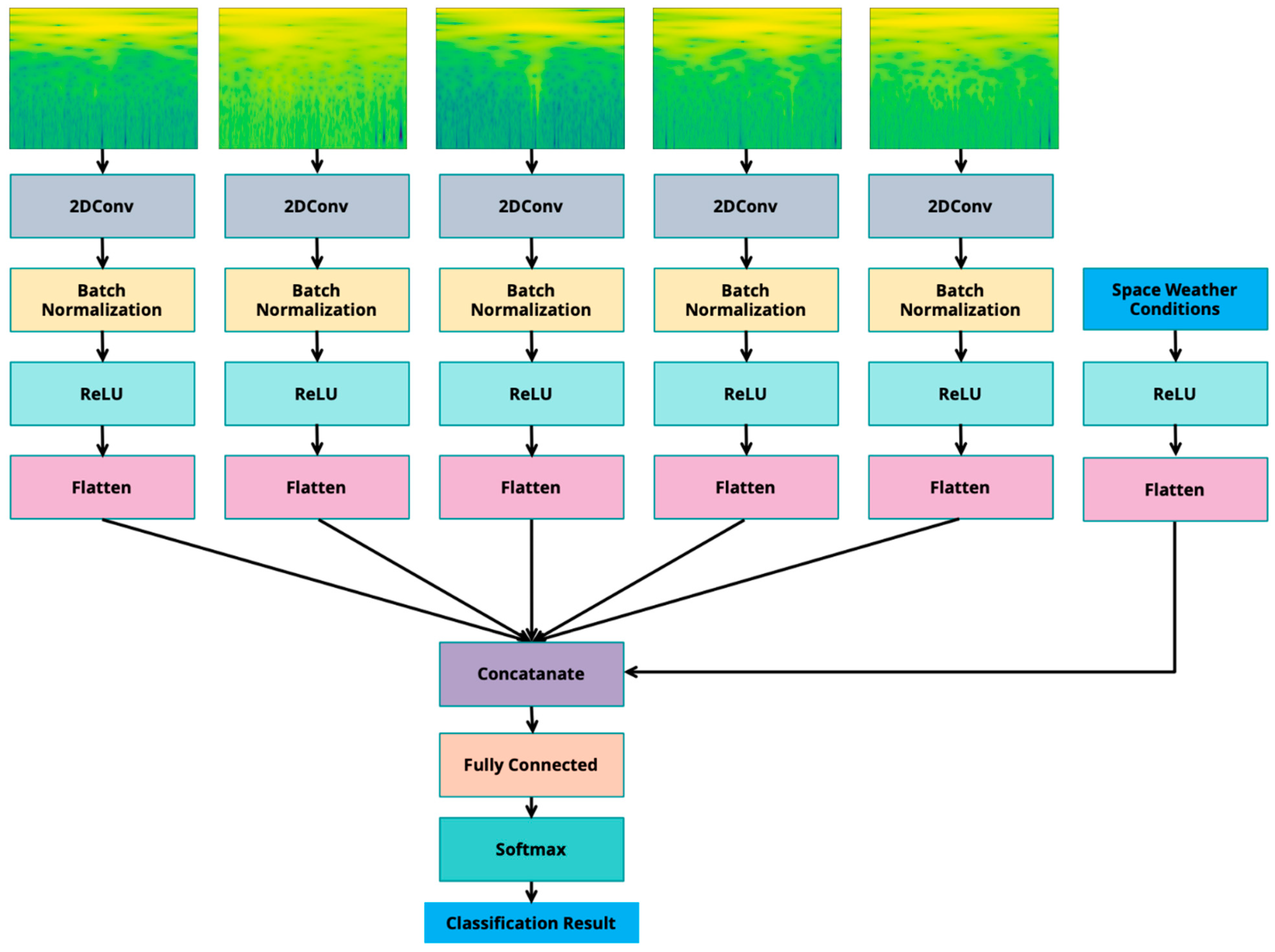
  • Five-day TEC and space weather indices are used dependently to detect the pre-earthquake and post-earthquake TEC and space weather indices. In other words, 5-day data is used as the input to the proposed CNN model simultaneously.
The study is divided into the following sections. In Section 2, the proposed method and related theories are presented in detail. The data collection, preprocessing, TEC image generation, and developed multi-input CNN model are described. The experimental works and the obtained results are detailed in Section 3. The parameters, data division, and training progress of the developed model are described. Finally, some concluding remarks and plans are given in Section 4.

2. Proposed Method

In Figure 1, the proposed method consists of three distinct stages: TEC and space weather indices-based data collection, preprocessing, and multi-input CNN-based classification.

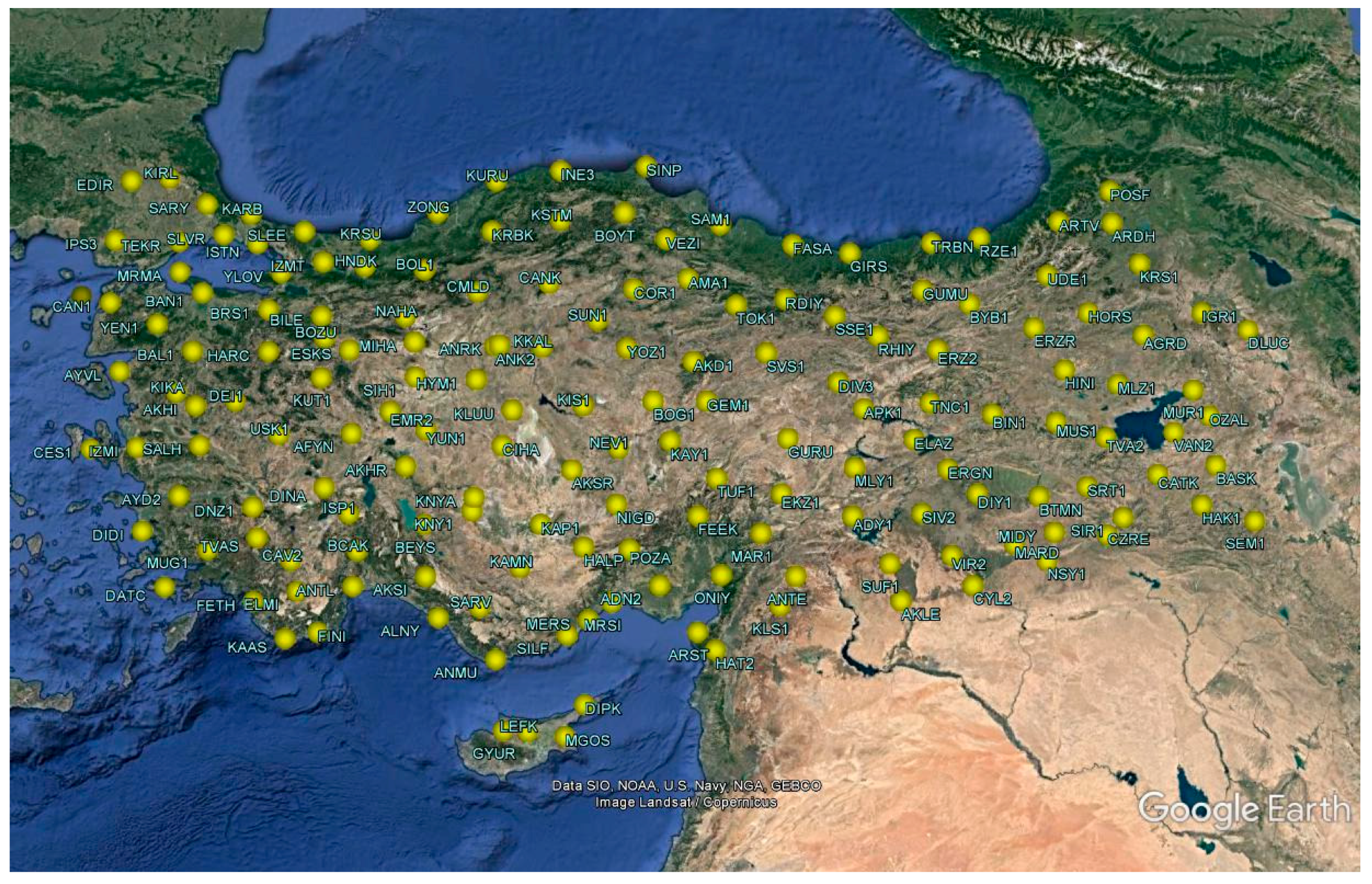
2.1. Data Collection
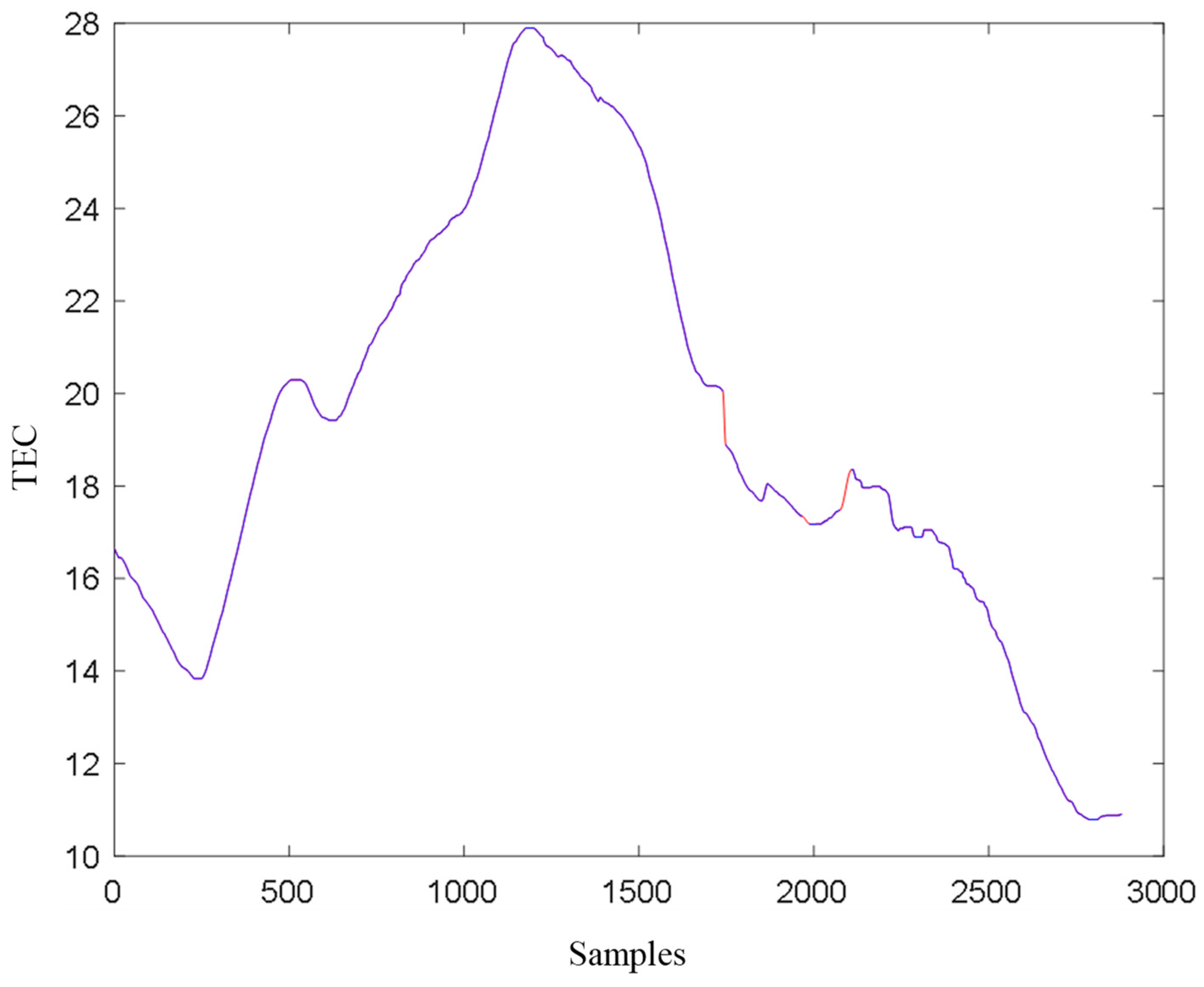
The ionospheric activity parameter that can be obtained using GPS/GNSS is the TEC. As mentioned above, the TEC is calculated as the integration of the number of ionospheric electrons in a region. This is achieved by measuring the time delay of electromagnetic waves sent from an observation point to a satellite or earth station at a given altitude range. This time delay is due to the high density of free electrons in the ionosphere and can be used to calculate the ionospheric TEC calculation. Although the ionospheric TEC is very sensitive to space weather conditions, solar and geomagnetic activities are the main factors causing unexpected anomalies. To say that the anomalies to be detected in the TEC time series are related to the earthquake, first and foremost, the space weather conditions should be analyzed in detail. In this context, in addition to TEC data, space weather indices such as the global geomagnetic index (Kp), the storm distribution time (Dst), the sunspot number (R), the geomagnetic storm index (Ap-index), the solar wind speed (Vsw), and the solar activity index (F10.7) are collected.
The TEC data are collected from the Turkish Continuously Operating Reference Stations, namely the TNPGN-Active network. TEC data from the last 15 years can be collected from 168 GNSS stations in this network. The TNPGN-Active network is a geocentric positioning system consisting of fixed GNSS stations and control centers for real-time positioning information, completed in May 2009. With the TNPGN-Active network, real-time geographic location information with centimeter accuracy can be obtained in a few seconds at any place and time in places where a sufficient number of GNSS satellites can be seen throughout Turkey and communication opportunities are possible. Figure 2 shows the distribution of stations belonging to the TNPGN-Active network on the map of Turkey. In addition, the space weather indices were downloaded from NASA’s OmniWeb Data Explorer (https://omniweb.gsfc.nasa.gov/form/dx1.html) (accessed on 4 July 2023).
The TEC data from stations located within Dobrovolsky’s earthquake preparation area (EPA) were utilized for each earthquake [59]. The EPA is calculated using the equation 10 0.43 M km. For instance, for an earthquake of magnitude Mw6, this value represents stations within a circle having a radius of approximately 380 km.

2.2. Preprocessing

As mentioned earlier, the TEC data are calculated based on the signal communication time between a GNSS receiver and its satellite. Because the ionospheric effect in GNSS signals depends on the signal frequency, TEC values can be obtained with the aid of any dual-frequency receiver. In some cases, TEC values cannot be calculated due to interruptions in the signals and gaps that occur in the TEC time series. In this case, the most appropriate values for missing TEC values are calculated with any interpolation method. Here, an interpolation method using the spline function [60], which provides an accurate estimation of missing data by creating a continuous function between each point in the dataset, was used to complete the missing TEC data. The polynomials used for the interpolation method using the spline function can be defined by the following equation:
s i x = a i + b i x x i + c i x x i 2 + d i x x i 3
where s i x denotes the polynomial between the points i and i + 1 . The coefficients   a i , b i , c i , and d i are determined according to certain boundary conditions and the values of two points. Determining the boundary conditions, combining the polynomials, and constructing the spline function are the steps that need to be performed correctly to complete the missing data in a given dataset. This method is frequently used in data analysis, especially by ensuring that the function between each point in the dataset is smooth. A drawing showing that the gaps are completed by the interpolation method for a TEC data series is given in Figure 3. The blue curve shows the obtained TEC data, while the red curve shows the completed TEC data. In Figure 3, while the blue curve indicates the TEC signal before the interpolation process, the red curve shows the TEC signal after the spline interpolation process. As shown in Figure 3, the missing parts of the TEC signal are appropriately completed.

2.3. Time–Frequency Image Representation of TEC Signal

A time–frequency representation is a mathematical tool that provides information about the frequency content of a signal as it evolves. It is used to analyze signals that are non-stationary, meaning their frequency content changes over time. Time–frequency representations provide information about which frequencies are present in a signal at different points in time. This allows for a more detailed analysis of signal components and their variations over time. The Continuous Wavelet Transform (CWT) is a mathematical operation that analyzes a signal in both the time and frequency domains using wavelet functions [61]. It is represented by the following equation:
W a , b = 1 a f x ψ x b a x
where W a , b indicates the wavelet coefficients, f x represents the input signal, ψ x denotes the complex conjugate wavelet function, and a and b are parameters that control the scale and translation of the wavelet function, respectively. By varying the values of a and b, the CWT captures different scales and positions of the frequency components present in the signal. Smaller values correspond to higher frequency resolutions and finer time localization, while larger values capture lower frequencies with coarser time localization. The CWT provides a time–frequency representation of the signal, showing how its frequency content changes over time. This representation can be visualized as a two-dimensional plot, often referred to as a time–frequency spectrogram or scalogram, where the y-axis represents frequency, the x-axis represents time, and the intensity or color indicates the magnitude of the frequency component. In Figure 4, the CWT images obtained for different TEC data are given.

2.4. Multi-Input Convolutional Neural Networks Model

A multi-input convolutional neural network (CNN) is a type of neural network architecture that processes multiple input sources simultaneously using convolutional layers [62]. Each input source can represent different types of data, such as images, text, audio, or any other form of structured or unstructured data. The basic idea behind a multi-input CNN is to extract features from each input source independently and then combine or fuse these features at later stages of the network to make predictions or perform a specific task. This approach allows the network to leverage the complementary information from different input sources and can lead to improved performance in tasks that require the integration of diverse data modalities. It is important to note that the specific architecture and design choices for a multi-input CNN can vary depending on the nature of the task and the characteristics of the input data. The fusion mechanism, in particular, plays a crucial role in determining how the features from different input sources are combined.
As shown in Figure 5, the 5-day time–frequency TEC images and space climate indices are provided as inputs to a multi-input CNN model. The nodes that take time–frequency images as input pass through convolution, batch normalization, rectified linear unit (ReLU), and flatten layers in sequence [63]. The convolutional layer is a commonly used layer type in neural network models. This layer applies a series of filters to the given input data and generates a set of feature maps as output. This operation is widely used, especially in areas such as image processing. The equation for the convolutional layer can be expressed as follows:
Y i , j , k = σ n = 1 N p = 1 P q = 1 Q W n , p , q , k X i + p 1 , j + q 1 , n
where X is the image given as the input to the convolution layer. The size of the input image is i × j × n , where i and j are the height and width of the input image, respectively, and n is the number of channels. Also, W is a set of tensors consisting of k filter matrices, each of size p × q × n. These filters are used to perform the convolution operation. It is the output feature map of the convolution layer, and the size of this matrix is i × j × k . Here, i and j represent the height and width of the output, respectively, while k represents the number of filters. The σ function is called the activation function and compresses the result of the convolution operation to output it. Various activation functions, such as ReLU and sigmoid, can be used. Batch normalization is a method used to normalize the output of any layer in a neural network model. This method calculates a scale factor to combine the mean and variance to zero for each batch of data during training.
These normalized outputs are then passed to an activation function. Batch normalization can be defined by the following equations:
μ B = 1 m i = 1 m x i
σ B 2 = 1 m i = 1 m x i μ B 2
x ^ i = x i μ B σ B 2 + ϵ
y i = γ x ^ i + β
where x i is the ith sample in a batch, μ B is the batch mean, and σ B 2 is the batch variance. x ^ i denotes the normalized output. γ and β are scale factors and bias parameters. ϵ is a small value used to avoid division by zero error. These equations show that the batch mean and variance are calculated, the normalized output is then obtained using these values, and, finally, the scale factor and bias terms are applied. This process can be used to normalize the output of any layer in a neural network model. Batch normalization helps neural networks perform better, often by providing a faster and more stable training process. ReLU is an activation function often used in neural network models. The ReLU function outputs the input value directly if the input value is greater than 0, while the output value is assigned 0 if the input value is less than 0. The ReLU function is mathematically expressed as
f x = max 0 , x
In Equation (8), x represents the input value and f x represents the output value. If the input x is positive, ReLU returns x as the output, and if the input x is negative or zero, ReLU returns 0 as the output. The ReLU function can be used as the activation function of any layer in a neural network model. Specifically, in deep neural network models, using the ReLU function creates less directional derivative (gradient) reduction problems for near-zero input values and provides faster learning. However, because the ReLU function produces an output of 0 for negative input values, in this case, a field with a positive input value and producing an output of zero (dying ReLU) may occur. This may limit the learning capacity of the network. To address this, variations like Leaky ReLU add a small slope to the negative part of the function, allowing a small gradient and preventing complete inactivity, thereby enhancing the network performance. A flatten layer is a layer that flattens the output of any previous layer in a neural network model, making it a single vector. This layer is often used especially for processing images as input. The flatten layer can be expressed by the following mathematical equations:
f l a t t e n X =   X
X i = X r , c , k
where X is a tensor from the previous layer. X′ is a flattened tensor. X r , c , k is the rth row, cth column, and kth channel value in the tensor. Equation (9) determines the order of each element in the tensor in the smoothed vector. A concatenate layer, which combines two or more tensors to form a new tensor, is located after flattening layers. This layer is especially used when more than one branch needs to be combined in neural network models or especially when the input data has different properties. Mathematically, the merged layer can be expressed by the following equations:
c o n c a t X 1 , X 2 , , X n = Y
where X 1 , X 2 , , X n are the tensors to combine and Y is the tensor to form. 1 , 2 , , n represent the number of channels of each tensor, respectively. The Fully Connected Layer is a neural network layer that generates another vector as output by subjecting the vector data received as input to a matrix multiplication process. This layer is usually used in the last layers and produces outputs that are used in tasks such as classification or regression. The mathematical equations for the fully connected layer are as follows:
y = σ W x + b
where x is an n-dimensional vector representing the input of the layer. W is the weight matrix and is m × n in size. m is the size of the output vector. b is the bias term and is an m-dimensional vector. σ is the activation function. The softmax layer is an output layer used in classification problems. It interprets the vector data received as input as probability values of classes and selects the most probable class. The softmax function is utilized to compute the probability value for each class by normalizing it relative to the total probabilities. The mathematical formulation of the softmax layer is expressed as follows:
y i = e z i j = 1 C e z j
where y i represents the probability value of class i. z i denotes the net output value of class i, and C signifies the total number of classes. The softmax function calculates the ratio of z i to e z i , reflecting the contribution of e z i to the overall probability of class C. Consequently, the probability of each class is proportioned to the total probabilities divided by the number of classes, ensuring that the sum of all the class probabilities equals 1. An important aspect of the softmax function is its adaptability to varying numbers of classes, enabling its application in diverse classification problems with different class counts.
The Classification Output is an output layer used in a classification problem. This layer calculates the probability values of the classes for a sample and performs the classification. The number of classes is determined as C and an output neuron is created for each class. Output neurons are converted to probability values using sigmoid, softmax, or other activation functions. In classification problems, the cross-entropy loss function is generally used. This function calculates the difference between the actual class label and the probability values predicted by the model. This difference is tried to be reduced to increase the accuracy of the model. The cross-entropy loss function can be expressed mathematically as
L = i = 1 C y i log y i ^
Here, y i is the real class label y i ^ and is the probability value predicted by the model. The cross-entropy loss is calculated by comparing the probability values of all the output neurons with the correct class label.

3. Experimental Works and Results

In the experimental studies, earthquakes of Mw5.0 and greater that occurred in Turkey between the years 2012 and 2019 were selected. We utilized data from GNSS stations in the CORS network to enhance the sensitivity to local ionospheric changes. However, there was a notable scarcity of data for TNPGN-Active prior to 2012, restricting our data collection to a limited time frame for the study. Additionally, due to the challenge of detecting seismo-ionospheric anomalies in earthquakes smaller than Mw5.0, only earthquakes of specific magnitudes were included in the dataset. These factors contribute to the study’s data limitations. The research focuses solely on Turkey within the mid-latitude region, characterized by fewer non-periodic fluctuations in ionospheric variation compared to high and low latitudes [64]. In the analysis of ionospheric anomalies in this region, the emphasis is placed on the strong correlation between the detected anomalies and earthquakes. Various earthquakes from the mentioned timeline are given in Table 1. The first two columns of Table 1 contain the location of the earthquakes, the third column contains the name of the earthquakes, and the fourth and fifth columns contain the date and magnitude of the earthquakes, respectively. The data on earthquakes were obtained from the United States Geological Survey (USGS) (https://earthquake.usgs.gov/earthquakes/search/) (accessed on 4 July 2023). In total, 5 days of TEC and space weather data before the earthquake from all TNPGN-Active GNSS stations within the EPA were recorded and labeled as “precursor days”. For example, for the MW5.2 Elazig earthquake, the Bingol, Malatya, Tunceli, Ergani, and Diyarbakir stations were used together with Elazig. The 5-day post-earthquake TEC and space weather data were collected from the same stations and labeled as “normal days”. In the test studies, it was seen that 5 days of TEC data were sufficient to capture a pattern in time series with deep learning. If the number of missing data in the TEC data is less than 20 samples, the missing data are completed with the spline function. Otherwise, the TEC data of the relevant day is not used. Thus, there were 175 samples in the “precursor days” class and 150 samples in the “normal days” class.
In addition to the TEC data, space weather data (Kp, Dst, Ap, R, Vsw, F10.7) for the days before and after the earthquakes were also recorded. While the Kp, Dst, and Ap indices indicate a geomagnetic storm condition, the R, Vsw, and F10.7 indices indicate solar activity levels. In total, 75% of the collected data were used to train the proposed multi-entry deep network architecture, and the remaining 25% of the data was used to test the trained network. In Figure 6 and Figure 7, the TEC images and space weather data produced for the “precursor days” and “normal days” classes are shown.
For performance evaluation, the accuracy, sensitivity, specificity, precision, and F1-score were used as performance measurement metrics. These metric results were obtained with true positive (TP), true negative (TN), false positive (FP), and false negative (FN) values in the confusion matrix. The mathematical definitions of these performance evaluation metrics were given using Equations (15)–(19).
A c c u r a c y = T P + T N T P + T N + F P + F N
S e n s i t i v i t y = T P T P + F N
S p e c i f i c i t y = T N T N + F P
P r e c i s i o n = T P T P + F P
F 1 s c o r e = 2 × T P 2 × T P + F P + F N
Accuracy provides a general measure of correctness by calculating the ratio of correctly predicted instances to the total number of instances. However, it may not be suitable for imbalanced datasets. Sensitivity focuses on the model’s ability to correctly identify positive instances, while specificity gauges its capability to correctly identify negative instances. Precision evaluates the accuracy of positive predictions, which is particularly important when the cost of false positives is high. The F1-score, being the harmonic mean of precision and sensitivity, strikes a balance between these metrics, making it especially valuable for evaluating models in situations where both false positives and false negatives carry significance, such as in imbalanced datasets.
In Figure 8, the architecture of the developed multi-input CNN model was implemented in MATLAB. As seen in Figure 8, after the 2D inputs, the convolution, batch normalization, ReLU, and flatten layers were sequenced. For the 1D input (input6), only the ReLU and flatten layers were sequenced. Then, all the flattened outputs were concatenated and fed into the fully connected layer. The classification was handled via the softmax and classification output layers, respectively.
In the convolution layers, 11 of the filters of size 3 × 3 were used, and in the training of the proposed multi-input CNN model, the ‘MiniBatchSize’ was set to 80 and the ‘MaxEpoches’ was selected as 50. In addition, the initial learning rate was set to 0.0001 and ‘Adam’ optimization was used.
In Figure 9, the training progress of the multi-input CNN model is depicted. Initially, the training accuracy hovered around 40%, while the test accuracy was approximately 55%. By the 90th iteration, the training accuracy reached 100%, and the test accuracy exceeded 80%, maintaining this level until the conclusion of the training process. Regarding the loss values, initially, the training dataset’s loss increased to around 100 but subsequently decreased to approximately 0, steadily decreasing after the 50th iteration. Similarly, the loss value for the test dataset reached approximately 0 by the 100th iteration and persisted at this level throughout the remaining training process. Notably, the training concluded after the 50th epoch and was completed in 7 min and 53 s, as displayed in Figure 9.
The confusion matrix, which was obtained for the test dataset, is shown in Figure 10. The rows show the true class outputs and the columns show the predicted outputs. In total, 83 of the “precursor days” samples and 59 of the “normal days” samples were correctly classified by the proposed multi-input CNN model, and the calculated accuracy score was 89.31%. In addition, 12 of the “precursor days” samples and 5 of the “normal days” samples were wrongly classified. Thus, the sensitivity, specificity, precision, and F1-score values were 94.32%, 83.10%, 87.37, and 90.71%, respectively. The calculated performance evaluation metrics are given in Table 2.
We conducted a comparison where various statistical measurements were employed. The TEC signals and the space weather indices were used in the extraction of the various statistical measurements, such as the minimum and maximum values, mean, and standard deviation. Additionally, a detailed examination of the data distribution was performed through the generation of a histogram with 30 bins, allowing us to discern key features of the dataset’s frequency distribution. Notably, the identification of the mode, represented by the bin center with the highest frequency, provided insights into the central tendencies of the data. Moreover, crucial percentiles (2.5th, 5th, 25th, 50th, 75th, 95th, and 97.5th) were calculated, shedding light on the data’s distribution and variability. The inclusion of entropy, kurtosis, and skewness as statistical metrics further contributed to our analysis. These measures offer insights into the dataset’s information content, shape of distribution tails, and asymmetry, providing a comprehensive understanding of its statistical profile. This multifaceted comparison of statistical metrics enhances our ability to characterize the dataset across various dimensions. This comprehensive comparison of statistical metrics offers a nuanced understanding of the dataset’s characteristics, ranging from central tendencies to dispersion, enabling a robust assessment of its overall statistical profile.
Various classical classifiers, namely decision tree, Support Vector Machine (SVM), and k-Nearest Neighbors (kNN), were employed in the classification process. The decision tree’s appeal lies in its interpretability and the ease with which it can handle both categorical and numerical features, making it particularly useful for understanding the decision-making process. Its hierarchical structure allows for transparent visualization, facilitating insights into feature importance and the logic behind classification decisions. Support Vector Machines (SVMs) excel in scenarios where the data is not linearly separable, as they transform the input space into a higher-dimensional one to discover a hyperplane that effectively separates classes. This capability makes SVMs robust in capturing intricate decision boundaries and handling complex relationships within the data. Additionally, the concept of the margin in SVMs contributes to better generalization performance, enhancing their applicability to various classification tasks. k-Nearest Neighbors (kNN) leverages the principle of locality, assuming that similar instances tend to fall into the same class. This method is especially effective in scenarios where instances of the same class are spatially clustered. The flexibility of kNN in adapting to the local structure of the data makes it a valuable choice for datasets with irregular decision boundaries and varying class distributions.
Table 3 presents a performance comparison of the proposed method against various statistical machine learning and deep learning approaches. The decision tree classifier achieves a moderate accuracy of 68.8%, highlighting potential limitations in capturing the dataset’s complexity. The SVM demonstrates improved accuracy at 80.6%, leveraging its strength in handling intricate decision boundaries. The kNN performs reasonably well with 74.2% accuracy, showcasing its suitability for datasets with localized patterns. We also designed a 3D CNN model for classifying daily spectrogram images with limited computing power or small datasets. The model has taken a 3D tensor of size [150 150 5 1] as the input, which was formed by stacking the images from each day. The model consisted of a 3D convolutional layer with 16 filters and ReLU activation, a batch normalization layer, a 3D max-pooling layer, a dropout layer, a fully connected layer with two output nodes, a softmax layer, and a classification output layer. The model was trained with stochastic gradient descent with momentum, with a mini-batch size of 16, an initial learning rate of 0.0001, and 20 epochs. The model performance was evaluated using the training and validation sets. The 3D CNN model produced an 83.6% accuracy score. Notably, the proposed method outperforms these classical classifiers, attaining the highest accuracy at 89.3%. This result suggests the efficacy of the proposed approach, indicating its potential as a robust solution for the specific classification task under consideration.

4. Conclusions

In this paper, an efficient deep learning model, namely the multi-input CNN approach, is applied to distinguish the “precursor days” and “normal days” of the ionospheric variation. Indeed, an earthquake precursor system is aimed to be designed using the deep learning model. In this context, TEC images and space weather indices are used as input to the designed multi-input CNN model. The model is trained in an end-to-end fashion, and the obtained results are evaluated using various performance evaluation metrics. According to the obtained results, the proposed method is able to classify the “precursor days” and “normal days” labeled with an 89.31% accuracy score. This accuracy rate is very promising for the near real-time detection of ionospheric changes as an earthquake precursor. Specifically, the high-level pattern of the TEC data in the days before earthquakes may be a harbinger of any upcoming earthquake with the aid of deep learning through an earthquake monitoring system to be established. In future studies, deeper multi-input CNN models will be designed to improve performance, and more datasets will be collected to test the developed model. In this article, the results obtained using limited data and the most basic multi-input CNN architecture are presented. As the amount of data increases, more complex network architectures can be designed. For this purpose:
(1)
To handle the increasing data size, we will add more layers to each network branch. Specifically, we will add a convolutional layer, a batch normalization layer, and a ReLU layer to each branch. The convolutional layer will apply a set of filters to the input to extract features. The batch normalization layer will normalize the output of the convolutional layer to improve the stability and speed of the training. The ReLU layer will apply a non-linear activation function to the output of the batch normalization layer to introduce non-linearity and sparsity to the network.
(2)
To improve the performance and robustness of the network, we will add skip connection layers to each deepened network branch. Skip connection layers are layers that connect the output of one layer to the input of another layer that is not adjacent to it. This way, the network can learn both local and global features and avoid the problem of vanishing gradients. Skip connection layers also help reduce overfitting by regularizing the network and preventing co-adaptation of features.
(3)
To enhance the collaboration and interaction among the network branches, we will add connection skip layers between different input branches of the network. Connection skip layers are layers that connect the output of one branch to the input of another branch that is not directly connected to it. This way, the network can learn from multiple sources of information and leverage the complementary and supplementary features from different branches. Connection skip layers also help train the branches jointly instead of separately and avoid the problem of branch divergence.
(4)
To increase the flexibility and adaptability of the network, we will add attention mechanisms to the network branches. Attention mechanisms are units that create direct connections between the input and the output of the network and assign different weights to different parts of the input based on the output. This way, the network can focus on the most relevant and informative parts of the input and ignore the irrelevant and noisy parts. Attention mechanisms also help simplify the network structure, reduce the number of parameters, and avoid the problem of overfitting.
(5)
In our future works, we will employ Grad-CAM (Gradient-weighted Class Activation Mapping) to gain insights into the model’s decision-making process, especially regarding false positives and negatives. Grad-CAM is a technique that visualizes the regions of an image that are important for a particular class prediction. It does so by leveraging the gradients of the target class concerning the final convolutional layer of the model. This provides a heat map highlighting the areas of the input image that contributed most to the model’s decision. By incorporating Grad-CAM into our analysis, we can pinpoint the regions of interest in instances where the model failed. This visualization not only helps in understanding the characteristics of misclassifications but also provides valuable insights into the features or patterns the model may be overlooking or misinterpreting.

Author Contributions

Conceptualization, H.U., E.Ş. and M.H.A.; methodology, S.T.A.O., M.K. and M.F.; software, H.U., E.Ş. and A.S.; validation, H.U., E.Ş. and M.H.A.; formal analysis, S.T.A.O., M.K. and M.F.; investigation, H.U., E.Ş. and A.S.; resources, H.U., E.Ş. and M.H.A.; data curation, S.T.A.O., M.K. and A.S.; writing—original draft preparation, H.U.; writing—review and editing, H.U., E.Ş., M.H.A., S.T.A.O., M.K., M.F. and A.S.; visualization, H.U., E.Ş. and M.H.A.; supervision, E.Ş. and A.S.; project administration, M.F. and A.S.; funding acquisition, M.F. and A.S. All authors have read and agreed to the published version of the manuscript.

Funding

This research was supported by the National Natural Science Foundation of China (NSFC) Research Fund for International Young Scientists, Grant no. 42250410331 and TUBITAK project number 123E372.

Data Availability Statement

The space weather indices were downloaded from NASA’s OMNIWeb Data Explorer. The observation data of the GNSS stations was authorized by the Turkish Continuously Operating Reference Stations.

Acknowledgments

The authors would like to thank the Turkish Continuously Operating Reference Stations for providing the observation data of the GNSS stations. In addition, the space weather indices were downloaded from NASA’s OMNIWeb Data Explorer, and it is available using this link: https://omniweb.gsfc.nasa.gov/form/dx1.html (accessed on 4 July 2023).

Conflicts of Interest

The authors declare no conflict of interest.

References

  1. Krasnov, V.M.; Drobzheva, Y.V. The acoustic field in the ionosphere caused by an underground nuclear explosion. J. Atmos. Sol. Terr. Phys. 2005, 67, 913–920. [Google Scholar] [CrossRef]
  2. Yiğit, E.; Koucká Knížová, P.; Georgieva, K.; Ward, W. A review of vertical coupling in the Atmosphere–Ionosphere system: Effects of waves, sudden stratospheric warmings, space weather, and of solar activity. J. Atmos. Sol. Terr. Phys. 2016, 141, 1–12. [Google Scholar] [CrossRef]
  3. Astafyeva, E. Ionospheric detection of natural hazards. Rev. Geophys. 2019, 57, 1265–1288. [Google Scholar] [CrossRef]
  4. Chen, J.; Zhang, X.; Ren, X.; Zhang, J.; Freeshah, M.; Zhao, Z. Ionospheric disturbances detected during a typhoon based on GNSS phase observations: A case study for typhoon Mangkhut over Hong Kong. Adv. Space Res. 2020, 66, 1743–1753. [Google Scholar] [CrossRef]
  5. Freeshah, M.; Osama, N.; Zhang, X. Using real GNSS data for ionospheric disturbance remote sensing associated with strong thunderstorm over Wuhan city. Acta Geod. Geophys. 2023. [Google Scholar] [CrossRef]
  6. Freeshah, M.; Zhang, X.; Chen, J.; Zhao, Z.; Osama, N.; Sadek, M.; Twumasi, N.; Twumasi, N. Detecting Ionospheric TEC Disturbances by Three Methods of Detrending through Dense CORS During A Strong Thunderstorm. Ann. Geophys. 2020, 63, GD667. [Google Scholar] [CrossRef]
  7. Freeshah, M.; Zhang, X.; Şentürk, E.; Adil, M.A.; Mousa, B.G.; Tariq, A.; Ren, X.; Refaat, M. Analysis of Atmospheric and Ionospheric Variations Due to Impacts of Super Typhoon Mangkhut (1822) in the Northwest Pacific Ocean. Remote Sens. 2021, 13, 661. [Google Scholar] [CrossRef]
  8. Kundu, B.; Senapati, B.; Matsushita, A.; Heki, K. Atmospheric wave energy of the 2020 August 4 explosion in Beirut, Lebanon, from ionospheric disturbances. Sci. Rep. 2021, 11, 2793. [Google Scholar] [CrossRef]
  9. Vesnin, A.; Yasyukevich, Y.; Perevalova, N.; Şentürk, E. Ionospheric Response to the 6 February 2023 Turkey–Syria Earthquake. Remote Sens. 2023, 15, 2336. [Google Scholar] [CrossRef]
  10. Leonard, R.S.; Barnes, R.A., Jr. Observation of ionospheric disturbances following the Alaska earthquake. J. Geophys. Res. 1965, 70, 1250–1253. [Google Scholar] [CrossRef]
  11. Yuen, P.C.; Weaver, P.F.; Suzuki, R.K.; Furumoto, A.S. Continuous, traveling coupling between seismic waves and the ionosphere evident in May 1968 Japan earthquake data. J. Geophys. Res. 1969, 74, 2256–2264. [Google Scholar] [CrossRef]
  12. Weaver, P.F.; Yuen, P.C.; Prolss, G.W.; Furumoto, A.S. Acoustic Coupling into the Ionosphere from Seismic Waves of the Earthquake at Kurile Islands on August 11, 1969. Nature 1970, 226, 1239–1241. [Google Scholar] [CrossRef] [PubMed]
  13. Pulinets, S.A. Strong earthquake prediction possibility with the help of topside sounding from satellites. Adv. Space Res. 1998, 21, 455–458. [Google Scholar] [CrossRef]
  14. Du, P.R.; Jiang, H.R.; Guo, J.S. Research on possibility of ionospheric anomalies as an earthquake precursor. Earthquake 1998, 18, 119. (In Chinese) [Google Scholar]
  15. Komjathy, A. Global Ionospheric Total Electron Content Mapping Using the Global Positioning System. Ph.D. Thesis, University of New Brunswick, Fredericton, NB, Canada, 1997. Department of Geodesy and Geomatics Engineering Technical Report No. 188. [Google Scholar]
  16. Afraimovich, E.L.; Astafieva, E.I.; Gokhberg, M.B.; Lapshin, V.M.; Permyakova, V.E.; Steblov, G.M.; Shalimov, S.L. Variations of the total electron content in the ionosphere from GPS data recorded during the Hector Mine earthquake of October 16, 1999, California. Russ. J. Earth Sci. 2004, 6, 339–354. [Google Scholar] [CrossRef]
  17. Liu, J.Y.; Chuo, Y.J.; Shan, S.J.; Tsai, Y.B.; Chen, Y.I.; Pulinets, S.A.; Yu, S.B. Pre-earthquake ionospheric anomalies registered by continuous GPS TEC measurements. Ann. Geophys. 2004, 22, 1585–1593. [Google Scholar] [CrossRef]
  18. Ulukavak, M.; Yalcinkaya, M. Precursor analysis of ionospheric GPS-TEC variations before the 2010 M7.2 Baja California earthquake. Geomat. Nat. Hazards Risk 2017, 8, 295–308. [Google Scholar] [CrossRef]
  19. Tariq, M.A.; Shah, M.; Hernández-Pajares, M.; Iqbal, T. Pre-earthquake ionospheric anomalies before three major earthquakes by GPS-TEC and GIM-TEC data during 2015–2017. Adv. Space Res. 2019, 63, 2088–2099. [Google Scholar] [CrossRef]
  20. Shah, M.; Abbas, A.; Adil, M.A.; Ashraf, U.; de Oliveira-Júnior, J.F.; Tariq, M.A.; Ahmed, J.; Ehsan, M.; Ali, A. Possible seismo-ionospheric anomalies associated with Mw > 5.0 earthquakes during 2000–2020 from GNSS TEC. Adv. Space Res. 2022, 70, 179–187. [Google Scholar] [CrossRef]
  21. Liu, J.Y.; Chen, Y.I.; Chen, C.H.; Liu, C.Y.; Chen, C.Y.; Nishihashi, M.; Li, J.Z.; Xia, Y.Q.; Oyama, K.I.; Hattori, K.; et al. Seismoionospheric GPS total electron content anomalies observed before the 12 May 2008 Mw7.9 Wenchuan earthquake. J. Geophys. Res. Space Phys. 2009, 114. [Google Scholar] [CrossRef]
  22. Pulinets, S.A.; Contreras, A.L.; Bisiacchi-Giraldi, G.; Ciraolo, L. Total eletron content variations in the ionosphere before the Colima, Mexico, earthquake of 21 January 2003. Geofísica Int. 2005, 44, 369–377. [Google Scholar] [CrossRef]
  23. Zakharov, V.I.; Kunitsyn, V.E. Regional features of atmospheric manifestations of tropical cyclones according to ground-based GPS network data. Geomagn. Aeron. 2012, 52, 533–545. [Google Scholar] [CrossRef]
  24. Dautermann, T.; Calais, E.; Haase, J.; Garrison, J. Investigation of ionospheric electron content variations before earthquakes in southern California, 2003–2004. J. Geophys. Res. Solid Earth 2007, 112, B02106. [Google Scholar] [CrossRef]
  25. Zhao, B.; Wang, M.; Yu, T.; Wan, W.; Lei, J.; Liu, L.; Ning, B. Is an unusual large enhancement of ionospheric electron density linked with the 2008 great Wenchuan earthquake? J. Geophys. Res. Space Phys. 2008, 113, A11304. [Google Scholar] [CrossRef]
  26. Yao, Y.; Chen, P.; Wu, H.; Zhang, S.; Peng, W. Analysis of ionospheric anomalies before the 2011 Mw 9.0 Japan earthquake. Chin. Sci. Bull. 2012, 57, 500–510. [Google Scholar] [CrossRef]
  27. Shah, M.; Jin, S. Statistical characteristics of seismo-ionospheric GPS TEC disturbances prior to global Mw ≥ 5.0 earthquakes (1998–2014). J. Geodyn. 2015, 92, 42–49. [Google Scholar] [CrossRef]
  28. Oikonomou, C.; Haralambous, H.; Muslim, B. Investigation of ionospheric TEC precursors related to the M7.8 Nepal and M8.3 Chile earthquakes in 2015 based on spectral and statistical analysis. Nat. Hazards 2016, 83, 97–116. [Google Scholar] [CrossRef]
  29. Nayak, K.; López-Urías, C.; Romero-Andrade, R.; Sharma, G.; Guzmán-Acevedo, G.M.; Trejo-Soto, M.E. Ionospheric Total Electron Content (TEC) Anomalies as Earthquake Precursors: Unveiling the Geophysical Connection Leading to the 2023 Moroccan 6.8 Mw Earthquake. Geosciences 2023, 13, 319. [Google Scholar] [CrossRef]
  30. Colonna, R.; Filizzola, C.; Genzano, N.; Lisi, M.; Tramutoli, V. Optimal Setting of Earthquake-Related Ionospheric TEC (Total Electron Content) Anomalies Detection Methods: Long-Term Validation over the Italian Region. Geosciences 2023, 13, 150. [Google Scholar] [CrossRef]
  31. Akhoondzadeh, M. Support vector machines for TEC seismo-ionospheric anomalies detection. Ann. Geophys. 2013, 31, 173–186. [Google Scholar] [CrossRef]
  32. Akhoondzadeh, M. A MLP neural network as an investigator of TEC time series to detect seismo-ionospheric anomalies. Adv. Space Res. 2013, 51, 2048–2057. [Google Scholar] [CrossRef]
  33. Akhoondzadeh, M. An Adaptive Network-based Fuzzy Inference System for the detection of thermal and TEC anomalies around the time of the Varzeghan, Iran, (Mw = 6.4) earthquake of 11 August 2012. Adv. Space Res. 2013, 52, 837–852. [Google Scholar] [CrossRef]
  34. Akhoondzadeh, M. Genetic algorithm for TEC seismo-ionospheric anomalies detection around the time of the Solomon (Mw = 8.0) earthquake of 06 February 2013. Adv. Space Res. 2013, 52, 581–590. [Google Scholar] [CrossRef]
  35. Akhoondzadeh, M. Thermal and TEC anomalies detection using an intelligent hybrid system around the time of the Saravan, Iran, (Mw = 7.7) earthquake of 16 April 2013. Adv. Space Res. 2014, 53, 647–655. [Google Scholar] [CrossRef]
  36. Akhoondzadeh, M. Investigation of GPS-TEC measurements using ANN method indicating seismo-ionospheric anomalies around the time of the Chile (Mw = 8.2) earthquake of 01 April 2014. Adv. Space Res. 2014, 54, 1768–1772. [Google Scholar] [CrossRef]
  37. Saqib, M.; Şentürk, E.; Sahu, S.A.; Adil, M.A. Comparisons of autoregressive integrated moving average (ARIMA) and long short term memory (LSTM) network models for ionospheric anomalies detection: A study on Haiti (Mw  =  7.0) earthquake. Acta Geod. Geophys. 2022, 57, 195–213. [Google Scholar] [CrossRef]
  38. Asaly, S.; Gottlieb, L.-A.; Inbar, N.; Reuveni, Y. Using Support Vector Machine (SVM) with GPS Ionospheric TEC Estimations to Potentially Predict Earthquake Events. Remote Sens. 2022, 14, 2822. [Google Scholar] [CrossRef]
  39. Akhoondzadeh, M. Firefly Algorithm in detection of TEC seismo-ionospheric anomalies. Adv. Space Res. 2015, 56, 10–18. [Google Scholar] [CrossRef]
  40. Akhoondzadeh, M. Application of Artificial Bee Colony algorithm in TEC seismo-ionospheric anomalies detection. Adv. Space Res. 2015, 56, 1200–1211. [Google Scholar] [CrossRef]
  41. Akhoondzadeh, M. Decision Tree, Bagging and Random Forest methods detect TEC seismo-ionospheric anomalies around the time of the Chile, (Mw = 8.8) earthquake of 27 February 2010. Adv. Space Res. 2016, 57, 2464–2469. [Google Scholar] [CrossRef]
  42. Akhoondzadeh, M. Kalman Filter, ANN-MLP, LSTM and ACO Methods Showing Anomalous GPS-TEC Variations Concerning Turkey&rsquos Powerful Earthquake (6 February 2023). Remote Sens. 2023, 15, 3061. [Google Scholar] [CrossRef]
  43. Aji, B.A.S.; Liong, T.H.; Muslim, B. Detection precursor of sumatra earthquake based on ionospheric total electron content anomalies using N-Model Articial Neural Network. In Proceedings of the 2017 International Conference on Advanced Computer Science and Information Systems (ICACSIS), Bali, Indonesia, 28–29 October 2017; pp. 269–276. [Google Scholar]
  44. Brum, D.; Veronez, M.R.; de Souza, E.; Koch, I.É.; Gonzaga, L.; Klein, I.; Matsuoka, M.T.; Francisco Rofatto, V.; Junior, A.M.; dos Reis Racolte, G.; et al. A Proposed Earthquake Warning System Based on Ionospheric Anomalies Derived From GNSS Measurements and Artificial Neural Networks. In Proceedings of the IGARSS 2019–2019 IEEE International Geoscience and Remote Sensing Symposium, Yokohama, Japan, 28 July 2019–2 August 2019; pp. 9295–9298. [Google Scholar]
  45. Akyol, A.A.; Arikan, O.; Arikan, F. A Machine Learning-Based Detection of Earthquake Precursors Using Ionospheric Data. Radio. Sci. 2020, 55, e2019RS006931. [Google Scholar] [CrossRef]
  46. Şentürk, E.; Saqib, M.; Adil, M.A. A Multi-Network based Hybrid LSTM model for ionospheric anomaly detection: A case study of the Mw 7.8 Nepal earthquake. Adv. Space Res. 2022, 70, 440–455. [Google Scholar] [CrossRef]
  47. Abri, R.; Artuner, H. LSTM-based deep learning methods for prediction of earthquakes using ionospheric data. GAZI Univ. J. Sci. 2022, 35, 1417–1431. [Google Scholar] [CrossRef]
  48. Lin, J.-W. Predicting ionospheric precursors before large earthquakes using neural network computing and the potential development of an earthquake early warning system. Nat. Hazards 2022, 113, 1519–1542. [Google Scholar] [CrossRef]
  49. Lin, J.-W. An adaptive Butterworth spectral-based graph neural network for detecting ionospheric total electron content precursor prior to the Wenchuan earthquake on 12 May 2008. Geocarto Int. 2022, 37, 14292–14308. [Google Scholar] [CrossRef]
  50. Tsai, T.C.; Jhuang, H.K.; Ho, Y.Y.; Lee, L.C.; Su, W.C.; Hung, S.L.; Lee, K.H.; Fu, C.C.; Lin, H.C.; Kuo, C.L. Deep Learning of Detecting Ionospheric Precursors Associated With M ≥ 6.0 Earthquakes in Taiwan. Earth Space Sci. 2022, 9, e2022EA002289. [Google Scholar] [CrossRef]
  51. Muhammad, A.; Külahcı, F. A semi-supervised total electron content anomaly detection method using LSTM-auto-encoder. J. Atmos. Sol. Terr. Phys. 2022, 241, 105979. [Google Scholar] [CrossRef]
  52. Xiong, P.; Long, C.; Zhou, H.; Zhang, X.; Shen, X. GNSS TEC-Based Earthquake Ionospheric Perturbation Detection Using a Novel Deep Learning Framework. IEEE J. Sel. Top. Appl. Earth Obs. Remote Sens. 2022, 15, 4248–4263. [Google Scholar] [CrossRef]
  53. Yue, Y.; Koivula, H.; Bilker-Koivula, M.; Chen, Y.; Chen, F.; Chen, G. TEC Anomalies Detection for Qinghai and Yunnan Earthquakes on 21 May 2021. Remote Sens. 2022, 14, 4152. [Google Scholar] [CrossRef]
  54. Draz, M.U.; Shah, M.; Jamjareegulgarn, P.; Shahzad, R.; Hasan, A.M.; Ghamry, N.A. Deep Machine Learning Based Possible Atmospheric and Ionospheric Precursors of the 2021 Mw 7.1 Japan Earthquake. Remote Sens. 2023, 15, 1904. [Google Scholar] [CrossRef]
  55. Karatay, S.; Gul, S.E. Prediction of GPS-TEC on Mw > 5 Earthquake Days Using Bayesian Regularization Backpropagation Algorithm. IEEE Geosci. Remote Sens. Lett. 2023, 20, 1–5. [Google Scholar] [CrossRef]
  56. Muhammad, A.; Külahcı, F.; Birel, S. Investigating radon and TEC anomalies relative to earthquakes via AI models. J. Atmos. Sol. Terr. Phys. 2023, 245, 106037. [Google Scholar] [CrossRef]
  57. Saqib, M.; Şentürk, E.; Sahu, S.A.; Adil, M.A. Ionospheric anomalies detection using autoregressive integrated moving average (ARIMA) model as an earthquake precursor. Acta Geophys. 2021, 69, 1493–1507. [Google Scholar] [CrossRef]
  58. Saqib, M.; Adil, M.A.; Freeshah, M. Pre-Earthquake Ionospheric Perturbation Analysis Using Deep Learning Techniques. Adv. Geomat. 2023, 1, 48–67. [Google Scholar] [CrossRef]
  59. Dobrovolsky, I.P.; Zubkov, S.I.; Miachkin, V.I. Estimation of the size of earthquake preparation zones. Pure Appl. Geophys. 1979, 117, 1025–1044. [Google Scholar] [CrossRef]
  60. Harder, R.L.; Desmarais, R.N. Interpolation using surface splines. J. Aircr. 1972, 9, 189–191. [Google Scholar] [CrossRef]
  61. Aguiar-Conraria, L.; Soares, M.J. The Contınuous Wavelet Transform: Movıng Beyond Unı-and Bıvarıate Analysıs. J. Econ. Surv. 2014, 28, 344–375. [Google Scholar] [CrossRef]
  62. Wei, Y.; Xia, W.; Lin, M.; Huang, J.; Ni, B.; Dong, J.; Zhao, Y.; Yan, S. HCP: A Flexible CNN Framework for Multi-Label Image Classification. IEEE Trans. Pattern Anal. Mach. Intell. 2016, 38, 1901–1907. [Google Scholar] [CrossRef]
  63. Li, Y.; Yuan, Y. Convergence Analysis of Two-Layer Neural Networks with ReLU Activation. In Neural Information Processing Systems; Guyon, I., Luxburg, U., Von Bengio, S., Wallach, H., Fergus, R., Vishwanathan, S., Garnett, R., Eds.; Curran Associates, Inc.: New York, NY, USA, 2017; Volume 30. [Google Scholar]
  64. He, Y.; Zhao, X.; Yang, D.; Wu, Y.; Li, Q. A study to investigate the relationship between ionospheric disturbance and seismic activity based on Swarm satellite data. Phys. Earth Planet. Inter. 2022, 323, 106826. [Google Scholar] [CrossRef]
Figure 1. The illustration of the proposed earthquake precursor detection system.
Remotesensing 15 05690 g001
Figure 2. The distribution of stations belonging to the TNPGN-Active network.
Remotesensing 15 05690 g002
Figure 3. The completion of the missing TEC values with the interpolation method.
Remotesensing 15 05690 g003
Figure 4. CWT time–frequency image representations for various TEC signals.
Remotesensing 15 05690 g004
Figure 5. The developed multi-input CNN model.
Remotesensing 15 05690 g005
Figure 6. 5-days TEC images.
Remotesensing 15 05690 g006
Figure 7. 5-day space weather indices.
Remotesensing 15 05690 g007
Figure 8. The architecture of the multi-input CNN model.
Remotesensing 15 05690 g008
Figure 9. The training progress of the multi-input CNN model.
Remotesensing 15 05690 g009
Figure 10. The obtained confusion matrix for the proposed method.
Remotesensing 15 05690 g010
Table 1. Some of the earthquakes that are considered in experimental works (USGS, 2023).
Lon (o)Lat (o)EarthquakeDateMw
42.27639.234Bulanık (Muş)2012-03-26T10:35:335
27.90440.863Marmara Denizi—[12.14 km] Marmaraereğlisi (Tekirdağ)2012-06-07T20:54:255.1
28.90736.530Akdeniz—[17.00 km] Fethiye (Muğla)2012-06-10T12:44:166
42.44437.157Silopi (Şırnak)2012-06-14T05:52:515.5
43.66738.733İpekyolu (Van)2012-06-24T20:07:215
28.93336.479Akdeniz—[16.38 km] Fethiye (Muğla)2012-06-25T13:05:285.3
28.85635.714Akdeniz—[75.07 km] Kaş (Antalya)2012-07-09T13:55:006
36.37137.574Andırın (Kahramanmaraş)2012-07-22T09:26:025
42.98037.464Uludere (Şırnak)2012-08-05T20:37:215.3
37.14037.284Pazarcık (Kahramanmaraş)2012-09-19T09:17:465.1
25.67039.680Ege Denizi—[37.56 km] Bozcaada (Çanakkale)2013-01-08T14:16:095.6
25.79040.303Ege Denizi—[12.01 km] Gökçeada (Çanakkale)2013-07-30T05:33:075.3
31.25736.692Akdeniz-Antalya Körfezi—[15.41 km] Manavgat (Antalya)2013-12-08T17:31:575
31.33236.048Akdeniz—[74.69 km] Alanya (Antalya)2013-12-28T15:21:036
25.28040.304Ege Denizi—[41.51 km] Gökçeada (Çanakkale)2014-05-24T09:25:016.5
30.93036.172Akdeniz—[48.08 km] Kumluca (Antalya)2014-09-04T21:00:035.2
26.27438.904Ege Denizi—[29.35 km] Karaburun (İzmir)2014-12-06T01:45:065.1
26.72834.864Akdeniz—[213.23 km] Datça (Muğla)2015-04-16T18:07:375.9
35.03636.565Akdeniz-Mersin Körfezi—[14.71 km] Karataş (Adana)2015-07-29T22:00:545
29.88536.185Akdeniz, Kekova Adası, Demre (Antalya)2015-10-06T21:27:345.2
37.82438.838Hekimhan (Malatya)2015-11-29T00:28:085
40.21739.261Kiğı (Bingöl)2015-12-02T23:27:075.3
34.35839.564Çiçekdağı (Kırşehir)2016-01-10T17:40:485
27.59736.405Ege Denizi—[32.95 km] Datça (Muğla)2016-09-27T20:57:095.2
26.13239.542Ayvacık (Çanakkale)2017-02-06T03:51:405.3
38.48737.596Samsat (Adıyaman)2017-03-02T11:07:255.5
28.64737.153Ula (Muğla)2017-04-13T16:22:165
27.81638.736Saruhanlı (Manisa)2017-05-27T15:53:235.1
26.31338.849Ege Denizi—[22.36 km] Karaburun (İzmir)2017-06-12T12:28:376.2
27.44436.920Ege Denizi—[12.00 km] Bodrum (Muğla)2017-07-20T22:31:096.5
27.62436.958Ege Denizi-Gökova Körfezi—[12.17 km] Bodrum (Muğla)2017-08-08T07:42:215.1
28.60537.115Ula (Muğla)2017-11-24T21:49:145.1
38.50437.584Samsat (Adıyaman)2018-04-24T00:34:295.1
31.21436.054Akdeniz—[76.70 km] Kumluca (Antalya)2018-09-12T06:21:465.2
28.05835.979Akdeniz—[72.62 km] Marmaris (Muğla)2019-01-24T14:30:525.1
26.42639.601Ayvacık (Çanakkale)2019-02-20T18:23:285
29.43437.440Acıpayam (Denizli)2019-03-20T06:34:275.5
39.12138.387Sivrice (Elazığ)2019-04-04T17:31:075.2
Table 2. Performance metrics of the proposed method.
Performance Evaluation MetricsValues
Accuracy (%)89.31
Sensitivity (%)94.32
Specificity (%)83.10
Precision (%)87.37
F1-score (%)90.71
Table 3. Performance comparison of proposed method with the various statistical machine learning and deep learning approaches.
ClassifierAccuracy (%)
Decision tree68.8
SVM80.6
kNN74.2
3D CNN83.6
Proposed89.3
Disclaimer/Publisher’s Note: The statements, opinions and data contained in all publications are solely those of the individual author(s) and contributor(s) and not of MDPI and/or the editor(s). MDPI and/or the editor(s) disclaim responsibility for any injury to people or property resulting from any ideas, methods, instructions or products referred to in the content.

