

High-Resolution Real-Time Coastline Detection Using GNSS RTK, Optical, and Thermal SfM Photogrammetric Data in the Po River Delta, Italy

Abstract
:1. Introduction
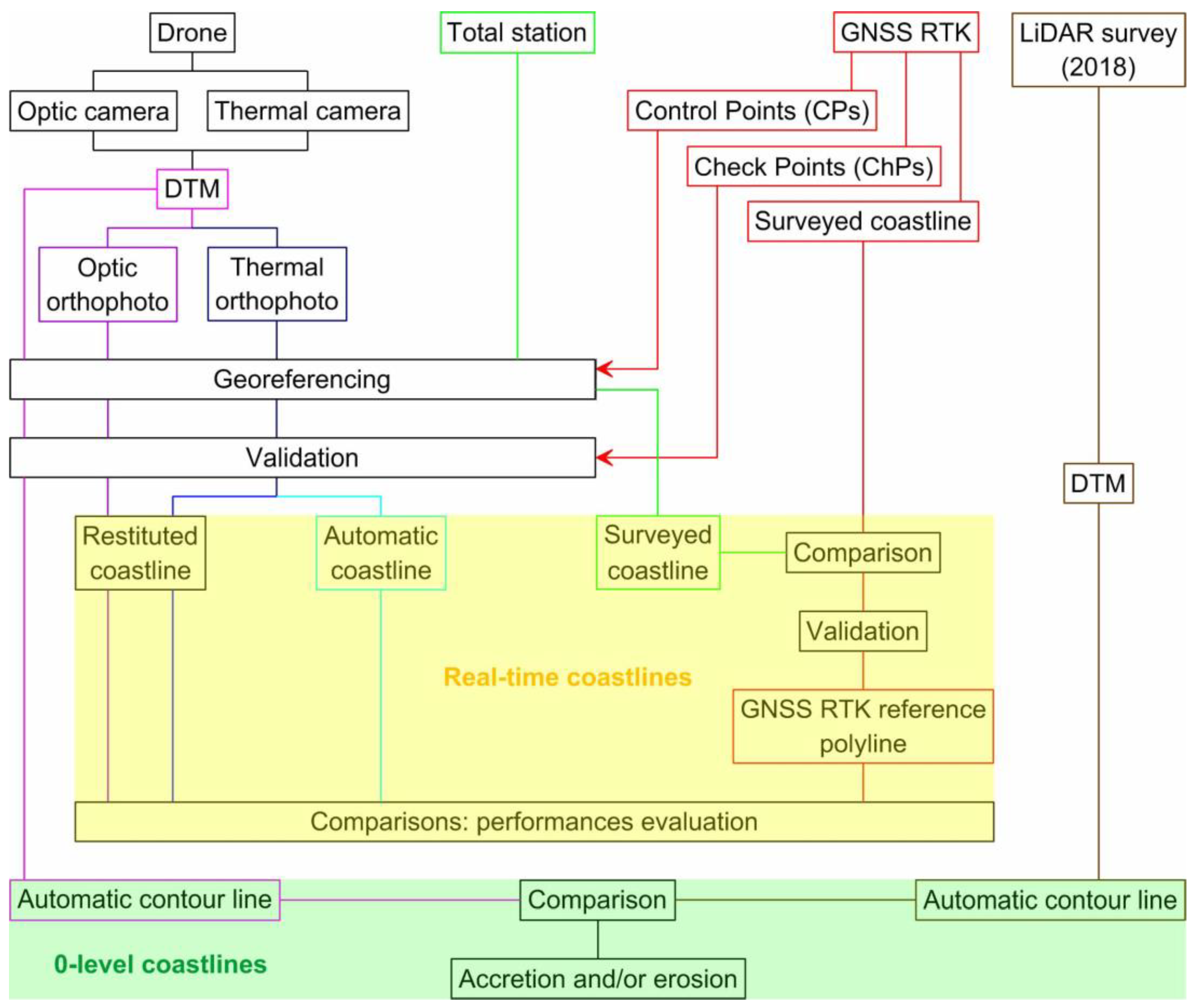
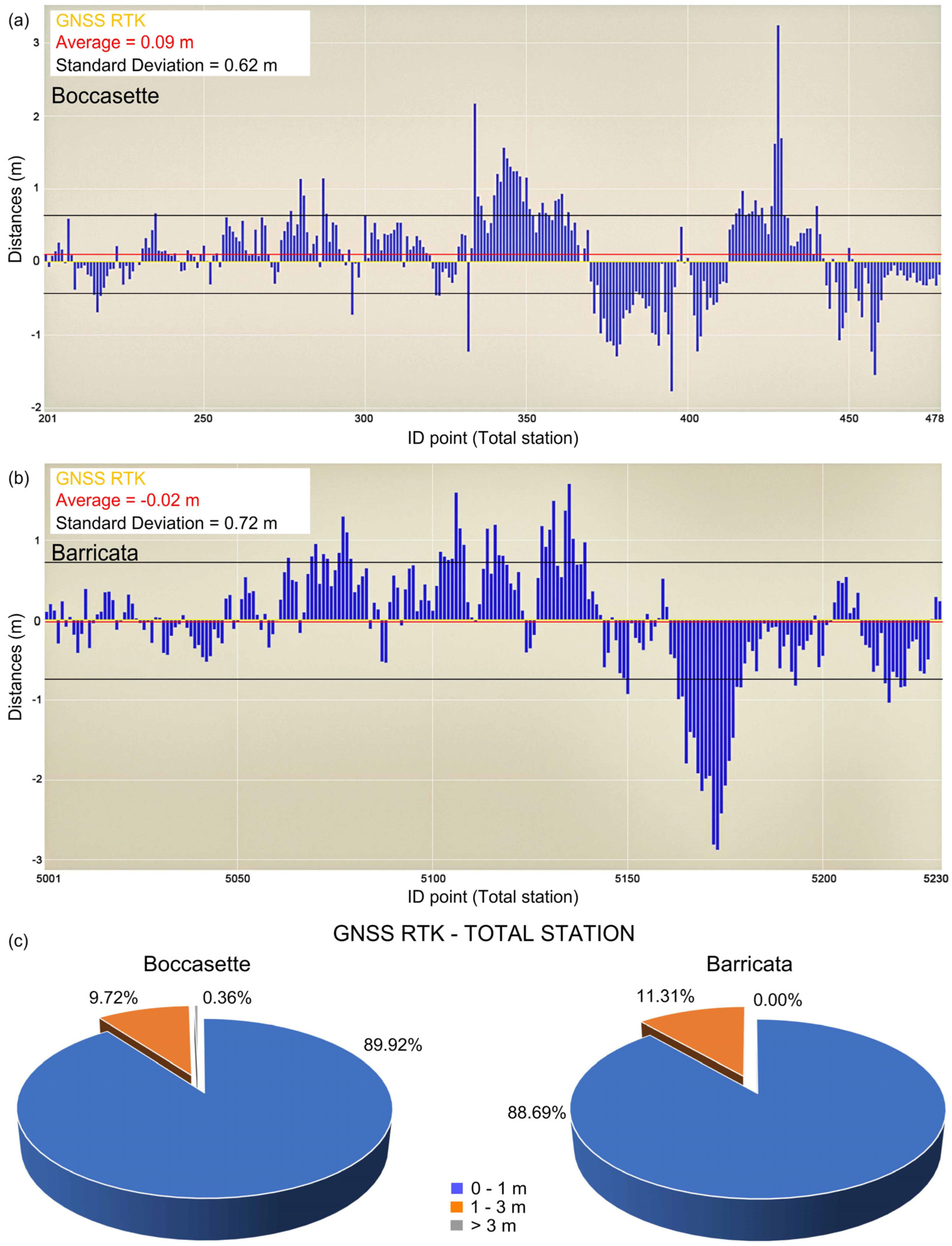
- Validation of the GNSS RTK real-time coastlines using the polylines measured with the total station;
- Extraction of the DTMs and orthophotos from optical and thermal photogrammetric data;
- Georeferencing and validation of the photogrammetric data;
- Restitution of the real-time coastlines on the optical and thermal orthophotos;
- Extraction of the automatic real-time coastline from the thermal orthophoto;
- Comparison between the reference GNSS RTK polylines with those obtained from the photogrammetric orthophotos, both in terms of distances and surfaces generated by polyline intersections;
- Evaluation of accuracies and performances of the different techniques;
- Extraction of the 0-level contour lines from the DTMs;
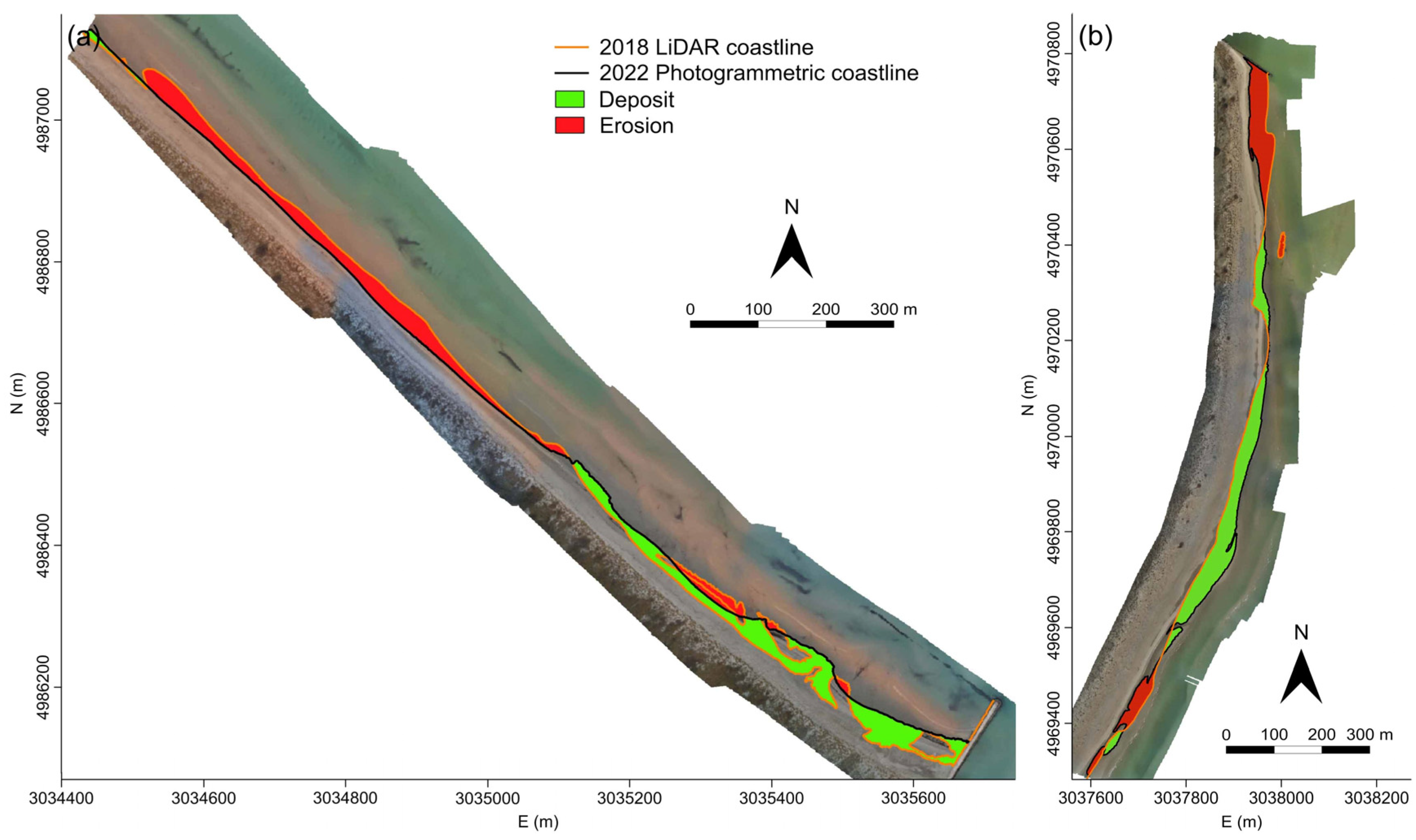
- Extraction of the 0-level contour lines from the DTM generated using an ALS (Airborne Laser Scanning) LiDAR survey conducted in 2018;
- Comparison between the obtained 0-level contour lines to evaluate modifications of the coastlines in terms of erosion and/or accretion in the 2018–2022 period.
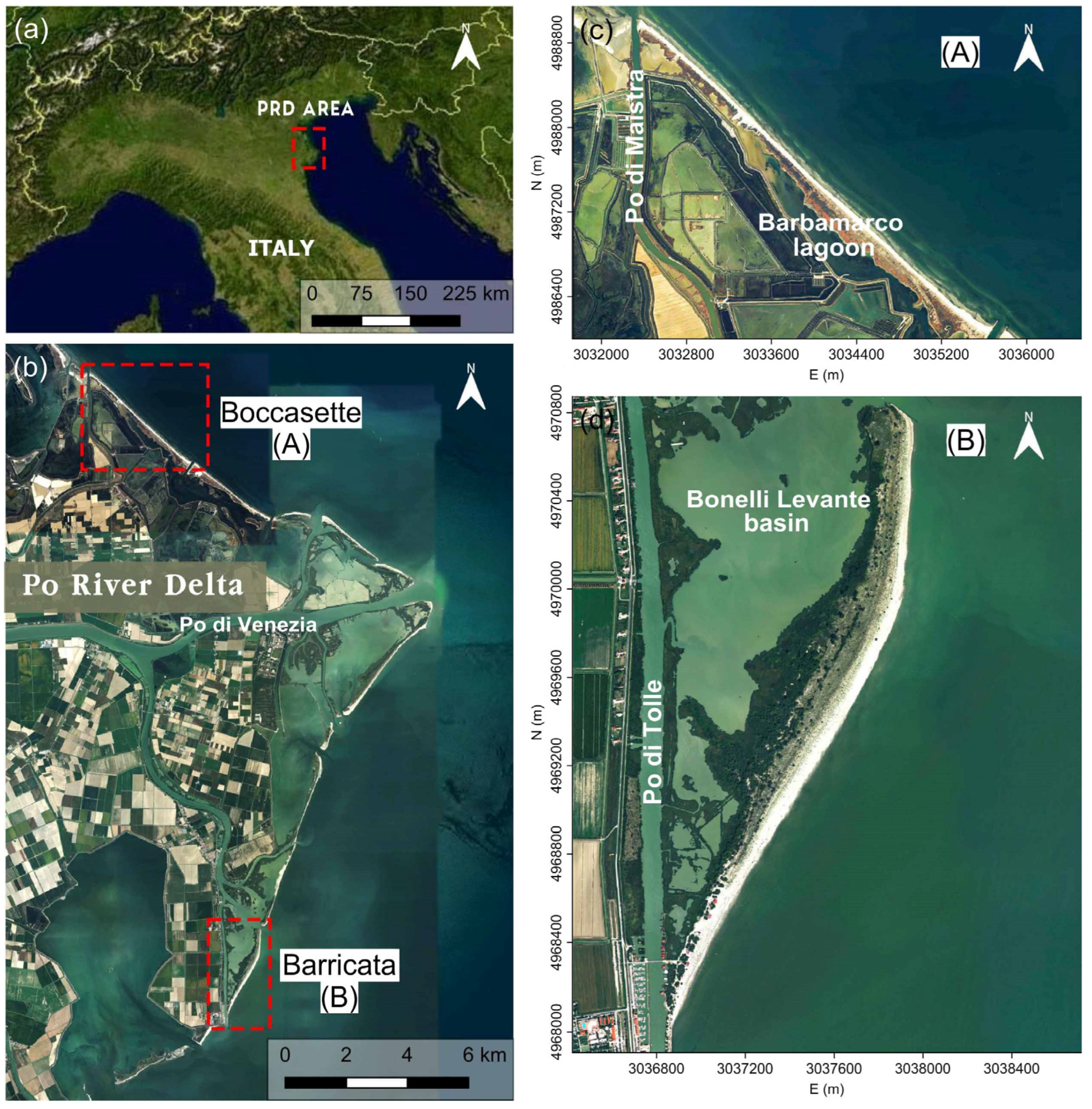
2. The Study Areas
3. Materials and Methods
3.1. The Surveys
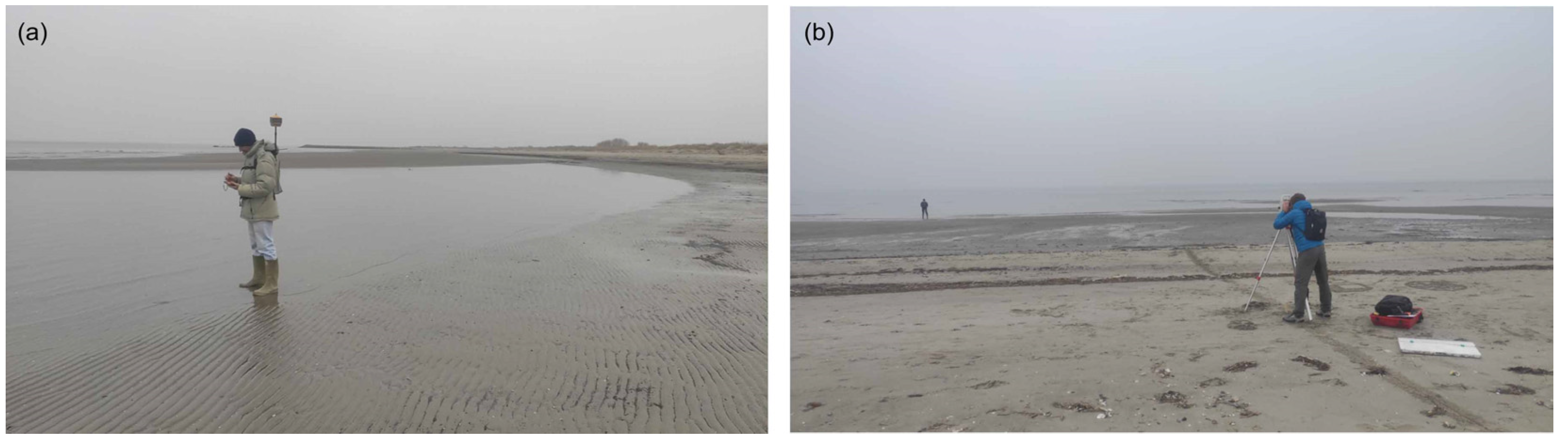
3.1.1. GNSS RTK and Classical Topographic Measurements
3.1.2. The 3D Photogrammetric Survey Using a Low-Cost Drone
3.2. The 2018 LiDAR Data
3.3. Processing and Comparisons
3.3.1. SfM Photogrammetric Images Processing
3.3.2. Automatic Real-Time Coastline Extraction from Thermal Images
3.3.3. Coastline Comparisons
3.3.4. Accretion/Erosion in the 2018–2022 Period
4. Results
4.1. Photogrammetric 3D Models and Orthophotos
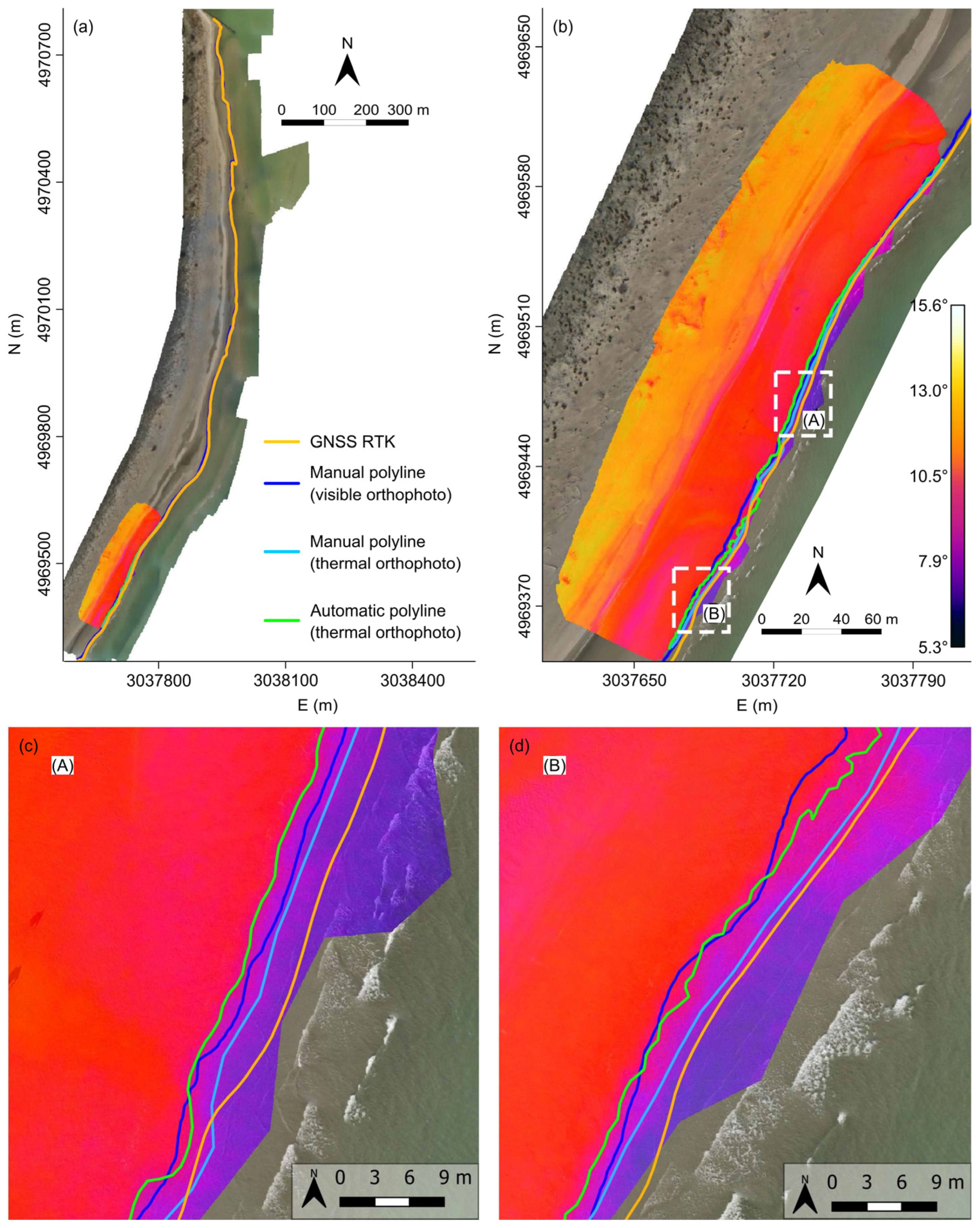
4.2. Restitution of Real-Time Coastlines by Visual Inspection
4.3. Automatic Real-Time Coastline Extraction
4.4. Real-Time Coastlines Comparisons
4.5. Multi-Temporal Coastlines Comparisons
5. Discussion
5.1. Analysis of the Results
5.2. Comparison with Previous Research Works
6. Conclusions
Author Contributions
Funding
Data Availability Statement
Acknowledgments
Conflicts of Interest
References
- Zhao, Q.; Pan, J.; Devlin, A.T.; Tang, M.; Yao, C.; Zamparelli, V.; Falabella, F.; Pepe, A. On the Exploitation of Remote Sensing Technologies for the Monitoring of Coastal and River Delta Regions. Remote Sens. 2022, 14, 2384. [Google Scholar] [CrossRef]
- Ericson, J.P.; Vörösmarty, C.J.; Dingman, S.L.; Ward, L.G.; Meybeck, M. Effective sea-level rise and deltas: Causes of change and human dimension implications. Glob. Planet. Chang. 2006, 50, 63–82. [Google Scholar] [CrossRef]
- Antonioli, F.; Anzidei, M.; Amorosi, A.; Lo Presti, V.; Mastronuzzi, G.; Deiana, G.; De Falco, G.; Fontana, A.; Fontolan, G.; Lisco, S.; et al. Sea-level rise and potential drowning of the Italian coastal plains: Flooding risk scenarios for 2100. Quat. Sci. Rev. 2017, 158, 29–43. [Google Scholar] [CrossRef]
- Kulp, S.A.; Strauss, B.H. New elevation data triple estimates of global vulnerability to sea-level rise and coastal flooding. Nat. Commun. 2019, 10, 4844. [Google Scholar] [CrossRef] [PubMed]
- Karami, E.; Alizadeh, N.; Farhadi, H.; Abdolazimi, H.; Maghsoudi, Y. Monitoring of land surface displacement based on SBAS-InSAR time-series and GIS techniques: A case study over the Shiraz Metropolis, Iran. ISPRS Ann. Photogramm. Remote Sens. Spatial Inf. Sci 2023, X-4/W1-202, 371–378. [Google Scholar] [CrossRef]
- Fiaschi, S.; Fabris, M.; Floris, M.; Achilli, V. Estimation of land subsidence in deltaic areas through differential SAR interferometry: The Po River Delta case study (Northeast Italy). Int. J. Remote Sens. 2018, 39, 8724–8745. [Google Scholar] [CrossRef]
- Saleh, M.; Becker, M. New estimation of Nile Delta subsidence rates from InSAR and GPS analysis. Environ. Earth Sci. 2018, 78, 6. [Google Scholar] [CrossRef]
- Tang, S.; Song, L.; Wan, S.; Wang, Y.; Jiang, Y.; Liao, J. Long-Time-Series Evolution and Ecological Effects of Coastline Length in Coastal Zone: A Case Study of the Circum-Bohai Coastal Zone, China. Land 2022, 11, 1291. [Google Scholar] [CrossRef]
- Vecchi, E.; Tavasci, L.; De Nigris, N.; Gandolfi, S. GNSS and Photogrammetric UAV Derived Data for Coastal Monitoring: A Case of Study in Emilia-Romagna, Italy. J. Mar. Sci. Eng. 2021, 9, 1194. [Google Scholar] [CrossRef]
- Eboigbe, M.A.; Kidner, D.B.; Thomas, M.; Thomas, N.; Aldwairy, H. Analysis of Low-Cost Uav Photogrammetry Solutions for Beach Modelling and Monitoring Using the Opensource Quantum Gis. In The International Archives of the Photogrammetry, Remote Sensing and Spatial Information Sciences, Proceedings of the ASPRS 2022 Annual Conference, Denver, CO, USA, 6–8 February and 21–25 March 2022; ISPRS: Hannover, Germany, 2022; Volume XLVI-M-2-2022. [Google Scholar]
- Fabris, M. Coastline evolution of the Po River Delta (Italy) by archival multi-temporal digital photogrammetry. Geomat. Nat. Hazards Risk 2019, 10, 1007–1027. [Google Scholar] [CrossRef]
- Alberico, I.; Cavuoto, G.; Di Fiore, V.; Punzo, M.; Tarallo, D.; Pelosi, N.; Ferraro, L.; Marsella, E. Historical maps and satellite images as tools for shoreline variations and territorial changes assessment: The case study of Volturno Coastal Plain (Southern Italy). J. Coast. Conserv. 2017, 22, 919–937. [Google Scholar] [CrossRef]
- Laksono, F.A.T.; Borzì, L.; Distefano, S.; Di Stefano, A.; Kovács, J. Shoreline Prediction Modelling as a Base Tool for Coastal Management: The Catania Plain Case Study (Italy). J. Mar. Sci. Eng. 2022, 10, 1988. [Google Scholar] [CrossRef]
- Fabris, M. Monitoring the Coastal Changes of the Po River Delta (Northern Italy) since 1911 Using Archival Cartography, Multi-Temporal Aerial Photogrammetry and LiDAR Data: Implications for Coastline Changes in 2100 A.D. Remote Sens. 2021, 13, 529. [Google Scholar] [CrossRef]
- Goksel, C.; Senel, G.; Dogru, A.O. Determination of shoreline change along the Black Sea coast of Istanbul using remote sensing and GIS technology. Desalination Water Treat. 2019, 177, 242–247. [Google Scholar] [CrossRef]
- Viana, R.D.; dos Reis, G.N.L.; Velame, V.M.G.; Körting, T.S. Shoreline extraction using unsupervised classification on Sentinel-2 imagery. In Proceedings of the XIX Brazilian Symposium on Remote Sensing, Santos, Brazil, 14–17 April 2019; Volume 19, p. 96606. [Google Scholar]
- Alcaras, E.; Amoroso, P.P.; Baiocchi, V.; Falchi, U.; Parente, C. Unsupervised classification based approach for coastline extraction from Sentinel-2 imagery. In Proceedings of the 2021 International Workshop on Metrology for the Sea; Learning to Measure Sea Health Parameters (MetroSea), Virtual Conference, 4–6 October 2021; pp. 423–427. [Google Scholar]
- Domazetović, F.; Šiljeg, A.; Marić, I.; Faričić, J.M.; Vassilakis, E.; Panđa, L. Automated Coastline Extraction Using the Very High-Resolution WorldView (WV) Satellite Imagery and Developed Coastline Extraction Tool (CET). Appl. Sci. 2021, 11, 9482. [Google Scholar] [CrossRef]
- Karaman, M. Comparison of thresholding methods for shoreline extraction from Sentinel-2 and Landsat-8 imagery: Extreme Lake Salda, track of Mars on Earth. J. Environ. Manag. 2021, 298, 113481. [Google Scholar] [CrossRef] [PubMed]
- McFeeters, S.K. The use of the Normalized Difference Water Index (NDWI) in the delineation of open water features. Int. J. Remote Sens. 1996, 17, 1425–1432. [Google Scholar] [CrossRef]
- Ma, M.; Wang, X.; Veroustraete, F.; Dong, L. Change in area of Ebinur Lake during the 1998 2005 period. Int. J. Remote Sens. 2007, 28, 5523–5533. [Google Scholar] [CrossRef]
- Wolf, A.F. Using WorldView-2 Vis–NIR Multispectral Imagery to Support Land Mapping and Feature Extraction Using Normalized Difference Index Ratios. In SPIE 8390, Algorithms and Technologies for Multispectral, Hyperspectral, and Ultraspectral Imagery XVIII, International Society for Optics and Photonics; SPIE: Bellingham, WA, USA, 2012; Volume 8390, p. 83900N. [Google Scholar] [CrossRef]
- Braga, F.; Tosi, L.; Prati, C.; Alberotanza, L. Shoreline detection: Capability of COSMO—SkyMed and high resolution multispectral images. Eur. J. Remote Sens. 2013, 46, 837–853. [Google Scholar] [CrossRef]
- Ma, H.; Guo, S.; Zhou, Y. Detection of Water Area Change Based on Remote Sensing Images. In GeoInformatics in Resource Management and Sustainable Ecosystem, Communications in Computer and Information Science; Bian, F., Xie, Y., Cui, X., Zeng, Y., Eds.; Springer: Berlin/Heidelberg, Germany, 2013; Volume 398. [Google Scholar]
- Liu, Y.; Wang, X.; Ling, F.; Xu, S.; Wang, C. Analysis of coastline extraction from Landsat-8 OLI imagery. Water 2017, 9, 816. [Google Scholar] [CrossRef]
- Burke, C.; Wich, S.; Kusin, K.; McAree, O.; Harrison, M.E.; Ripoll, B.; Ermiasi, Y.; Mulero-Pázmány, M.; Longmore, S. Thermal-Drones as a Safe and Reliable Method for Detecting Subterranean Peat Fires. Drones 2019, 3, 23. [Google Scholar] [CrossRef]
- Burke, C.; Rashman, M.; Wich, S.; Symons, A.; Theron, C.; Longmore, S. Optimising observing strategies for monitoring animals using drone-mounted thermal infrared cameras. Int. J. Remote Sens. 2019, 40, 439–467. [Google Scholar] [CrossRef]
- Povlsen, P.; Linder, A.C.; Larsen, H.L.; Durdevic, P.; Arroyo, D.O.; Bruhn, D.; Pertoldi, C.; Pagh, S. Using Drones with Thermal Imaging to Estimate Population Counts of European Hare (Lepus europaeus) in Denmark. Drones 2023, 7, 5. [Google Scholar] [CrossRef]
- Maurya, N.K.; Tripathi, A.K.; Chauhan, A.; Pandey, P.C.; Lamine, S. Recent Advancement and Role of Drones in Forest Monitoring: Research and Practices. In Advances in Remote Sensing for Forest Monitoring; Arellano, P., Pandey, P.C., Eds.; Wiley: Hoboken, NJ, USA, 2022; pp. 223–254. [Google Scholar]
- Rouze, G.; Neely, H.; Morgan, C.; Kustas, W.; Wiethorn, M. Evaluating unoccupied aerial systems (UAS) imagery as an alternative tool towards cotton-based management zones. Precis. Agric. 2021, 22, 1861–1889. [Google Scholar] [CrossRef]
- Dahaghin, M.; Samadzadegan, F.; Javan, F.D. Precise 3D extraction of building roofs by fusion of UAV-based thermal and visible images. Int. J. Remote Sens. 2021, 42, 7002–7030. [Google Scholar] [CrossRef]
- Hou, Y.; Chen, M.; Volk, R.; Soibelman, L. Investigation on performance of RGB point cloud and thermal information data fusion for 3D building thermal map modeling using aerial images under different experimental conditions. J. Build. Eng. 2022, 45, 103380. [Google Scholar] [CrossRef]
- Zanutta, A.; Lambertini, A.; Vittuari, L. UAV Photogrammetry and Ground Surveys as a Mapping Tool for Quickly Monitoring Shoreline and Beach Changes. J. Mar. Sci. Eng. 2020, 8, 52. [Google Scholar] [CrossRef]
- Michałowska, K.; Głowienka, E. Multi-Temporal Analysis of Changes of the Southern Part of the Baltic Sea Coast Using Aerial Remote Sensing Data. Remote Sens. 2022, 14, 1212. [Google Scholar] [CrossRef]
- Romagnoli, C.; Bosman, A.; Casalbore, D.; Anzidei, M.; Doumaz, F.; Bonaventura, F.; Meli, M.; Verdirame, C. Coastal Erosion and Flooding Threaten Low-Lying Coastal Tracts at Lipari (Aeolian Islands, Italy). Remote Sens. 2022, 14, 2960. [Google Scholar] [CrossRef]
- Teatini, P.; Tosi, L.; Strozzi, T. Quantitative evidence that compaction of Holocene sediments drives the present land subsidence of the Po Delta, Italy. J. Geophys. Res. 2011, 116, B08407. [Google Scholar] [CrossRef]
- Corbau, C.; Simeoni, U.; Zoccarato, C.; Mantovani, G.; Teatini, P. Coupling land use evolution and subsidence in the Po Delta, Italy: Revising the past occurrence and prospecting the future management challenges. Sci. Total Environ. 2019, 654, 1196–1208. [Google Scholar] [CrossRef] [PubMed]
- Farolfi, G.; Bianchini, S.; Casagli, N. Integration of GNSS and satellite InSAR data: Derivation of fine-scale vertical surface motion maps of Po Plain, Northern Apennines, and Southern Alps, Italy. IEEE Trans. Geosci. Remote Sens. 2019, 57, 319–328. [Google Scholar] [CrossRef]
- Cenni, N.; Fiaschi, S.; Fabris, M. Monitoring of Land Subsidence in the Po River Delta (Northern Italy) Using Geodetic Networks. Remote Sens. 2021, 13, 1488. [Google Scholar] [CrossRef]
- Fabris, M.; Battaglia, M.; Chen, X.; Menin, A.; Monego, M.; Floris, M. An Integrated InSAR and GNSS Approach to Monitor Land Subsidence in the Po River Delta (Italy). Remote Sens. 2022, 14, 5578. [Google Scholar] [CrossRef]
- Carlo, C. Physical Processes and Human Activities in the Evolution of the Po Delta, Italy. J. Coast. Res. 1998, 14, 775–793. [Google Scholar]
- Correggiari, A.; Cattaneo, A.; Trincardi, F. The modern Po Delta system: Lobe switching and asymmetric prodelta growth. Mar. Geol. 2005, 222–223, 49–74. [Google Scholar] [CrossRef]
- Simeoni, U.; Corbau, C. A review of the Delta Po evolution (Italy) related to climatic changes and human impacts. Geomorphology 2009, 107, 64–71. [Google Scholar] [CrossRef]
- Municipality of Venice, Centro Previsioni e Segnalazioni Maree. Available online: https://www.comune.venezia.it/it/content/centro-previsioni-e-segnalazioni-maree (accessed on 24 February 2022).
- Agisoft LLC. Agisoft Metashape User Manual; Professional Edition, Version 1.8; Agisoft LLC: St. Petersburg, Russia, 2022. [Google Scholar]
- Agisoft LLC. Metashape Python Reference, Release 1.8.2; Agisoft LLC: St. Petersburg, Russia, 2022. [Google Scholar]
- Fabris, M.; Fontana Granotto, P.; Monego, M. Expeditious Low-Cost SfM Photogrammetry and a TLS Survey for the Structural Analysis of Illasi Castle (Italy). Drones 2023, 7, 101. [Google Scholar] [CrossRef]
- Nagendra, H.; Gadgil, M. Biodiversity Assessment at Multiple Scales: Linking Remotely Sensed Data with Field Information. Proc. Natl. Acad. Sci. USA 1999, 96, 9154–9158. [Google Scholar] [CrossRef]
- Maglione, P.; Parente, C.; Santamaria, R.; Vallario, A. Modelli Tematici 3D Della Copertura Del Suolo a Partire Da DTM Immagini Telerilevate Ad Alta Risoluzione WorldView-2. Rend. Online Della Soc. Geol. Ital. 2014, 30, 33–40. [Google Scholar] [CrossRef]
- Alcaras, E.; Falchi, U.; Parente, C.; Vallario, A. Accuracy Evaluation for Coastline Extraction from Pléiades Imagery Based on NDWI and IHS Pan-Sharpening Application. Appl. Geomat. 2022, 15, 595–605. [Google Scholar] [CrossRef]
- Lee, J.M.; Park, J.-Y.; Choi, J.-Y. Evaluation of sub-aerial topographic surveying techniques using total station and RTK-GPS for application in macrotidal sand beach environment. J. Coast. Res. 2013, 65, 535–540. [Google Scholar] [CrossRef]
- Marchel, Ł.; Specht, M. Method for Determining Coastline Course Based on Low-Altitude Images Taken by a UAV. Remote Sens. 2023, 15, 4700. [Google Scholar] [CrossRef]
- El Kafrawy, S.; Basiouny, M.; Ghanem, E.; Taha, A. Performance evaluation of shoreline extraction methods based on remote sensing data. J. Geogr. Environ. Earth Sci. Int. 2017, 11, 1–18. [Google Scholar] [CrossRef]


| 3D Model | N. CPs | N. ChPs | RMSE (cm) | |
|---|---|---|---|---|
| CPs | ChPs | |||
| Boccasette | 24 | 8 | 4.1 | 4.9 |
| Barricata | 22 | 7 | 3.5 | 3.8 |
| Comparisons | Length (m) | RI | DRI | |||
|---|---|---|---|---|---|---|
| Min (m) | Max (m) | Average (m) | St. Dev. (m) | |||
| GNSS – Total station (i) | 635.73 | 0.47 | 0.00 | 0.78 | 0.21 | 0.21 |
| GNSS – Restitution (optical) (ii) | 635.73 | 4.67 | 0.03 | 6.08 | 2.63 | 2.77 |
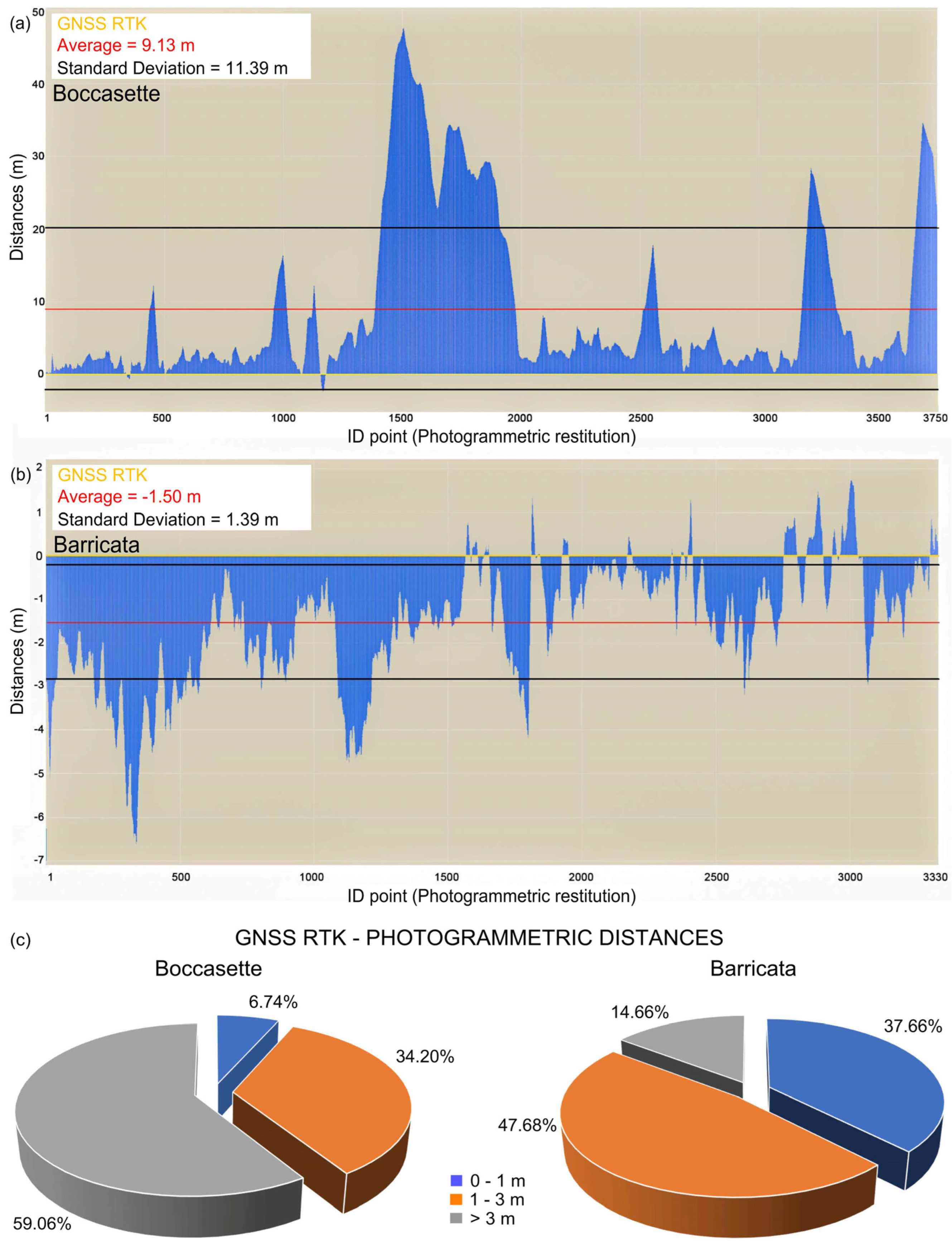
| GNSS – Restitution (optical) (iii) | 2628.52 | 8.81 | 0.03 | 10.60 | 4.09 | 3.75 |
| Comparisons | Length (m) | RI | DRI | |||
|---|---|---|---|---|---|---|
| Min (m) | Max (m) | Average (m) | St. Dev. (m) | |||
| GNSS – Total station (i) | 563.79 | 0.52 | 0.01 | 0.99 | 0.22 | 0.22 |
| GNSS – Restitution (optical) (ii) | 563.80 | 0.93 | 0.02 | 1.43 | 0.46 | 0.38 |
| GNSS – Restitution (optical) (iii) | 1649.78 | 1.63 | 0.02 | 2.41 | 0.52 | 0.55 |
| GNSS – Restitution (optical) (iv) | 281.30 | 2.90 | - | - | - | - |
| GNSS – Restitution (thermal) (v) | 281.30 | 1.29 | 0.22 | 1.49 | 0.89 | 0.56 |
| GNSS – Automatic (thermal) (vi) | 281.30 | 2.76 | 0.08 | 3.53 | 1.18 | 1.36 |
Disclaimer/Publisher’s Note: The statements, opinions and data contained in all publications are solely those of the individual author(s) and contributor(s) and not of MDPI and/or the editor(s). MDPI and/or the editor(s) disclaim responsibility for any injury to people or property resulting from any ideas, methods, instructions or products referred to in the content. |
© 2023 by the authors. Licensee MDPI, Basel, Switzerland. This article is an open access article distributed under the terms and conditions of the Creative Commons Attribution (CC BY) license (https://creativecommons.org/licenses/by/4.0/).
Share and Cite
Fabris, M.; Balin, M.; Monego, M. High-Resolution Real-Time Coastline Detection Using GNSS RTK, Optical, and Thermal SfM Photogrammetric Data in the Po River Delta, Italy. Remote Sens. 2023, 15, 5354. https://doi.org/10.3390/rs15225354
Fabris M, Balin M, Monego M. High-Resolution Real-Time Coastline Detection Using GNSS RTK, Optical, and Thermal SfM Photogrammetric Data in the Po River Delta, Italy. Remote Sensing. 2023; 15(22):5354. https://doi.org/10.3390/rs15225354
Chicago/Turabian StyleFabris, Massimo, Mirco Balin, and Michele Monego. 2023. "High-Resolution Real-Time Coastline Detection Using GNSS RTK, Optical, and Thermal SfM Photogrammetric Data in the Po River Delta, Italy" Remote Sensing 15, no. 22: 5354. https://doi.org/10.3390/rs15225354