A Method of Extracting the SWH Based on a Constituted Wave Slope Feature Vector (WSFV) from X-Band Marine Radar Images

Abstract

The shadow statistical method (SSM) used for extracting the significant wave height (SWH) from X-band marine radar images was further investigated because of its advantage of not requiring an external reference for calibration. Currently, a fixed shadow segmentation threshold is utilized to extract the SWH from a radar image based on the SSM. However, the retrieval accuracy of the SWH is not ideal for low wind speeds since the echo intensity of sea waves rapidly decays over distance. In order to solve this problem, an adaptive shadow threshold, which varies with echo intensity over distance and can accurately divide the radar image into shadow and nonshadow areas, is adopted to calculate the wave slope (WS) based on the texture feature of the edge image. Instead of using the averaged WS, the wave slope feature vector (WSFV) is constructed for retrieving the SWH since the illumination ratio and the calculated WS in the azimuth are different for shore-based radar images. In this paper, the SWH is calculated based on the constructed WSFV and classical support vector regression (SVR) technology. The collected 222 sets of X-band marine radar images with an SWH range of 1.0∼3.5 m and an average wind speed range of 5∼10 m/s were utilized to verify the performance of the proposed approach. The buoy record, which was deployed during the experiment, was used as the ground truth. For the proposed approach, the mean bias (BIAS) and the mean absolute error (MAE) were 0.03 m and 0.14 m when the ratio of the training set to the test set was 1:1. Compared to the traditional SSM, the correlation coefficient (CC) of the proposed approach increased by 0.27, and the root mean square error (RMSE) decreased by 0.28 m.

1. Introduction

To understand the evolution law of a sea wave, it is particularly important to extract the significant wave height (SWH), since the SWH is a key technical indicator for characterizing the wave energy [1,2,3]. Recently, noncoherent X-band marine radar images have been utilized for retrieving sea wave parameters due to the low cost of marine radar and the radar data containing abundant sea clutter information [4,5]. Currently, the research on retrieving the SWH from X-band radar images is mainly conducted under high wind speeds. Under low-wind-speed conditions, improving the SWH inversion accuracy can more accurately evaluate the impact of waves on marine ecosystems and marine energy development, ensuring the safety of ship navigation and capturing the evolution processes of waves.

The lower waves are blocked by the higher waves, and the shadow areas are generated in the radar image because of the fluctuation in the sea surface [6,7]. Meanwhile, the echo intensity of the sea wave decays along with increase in the distance to the radar antenna. The shadowing is dominant for the achieved radar image when the electromagnetic wave emitted grazes into the sea surface [8]. Nowadays, the spectral analysis approach based on Fourier transform and the shadow statistical method (SSM) (using shadow statistics) are the primary technologies for retrieving the SWH from X-band marine radar images [9]. In addition, ensemble empirical mode decomposition [4] and support vector regression (SVR) technology [10,11] are used to estimate the SWH since the shadowing of radar images depends on the sea conditions and the building height of the radar antenna.

For the three-dimensional (3D) Fourier spectral analysis approach, the image spectrum is achieved by using the 3D Fourier transform on the selected analysis area of a radar image sequence [12]. The SWH is obtained by using the linear relation to the root mean square (RMS) of the extracted signal-to-noise ratio (SNR) [13]. However, external measuring instruments, such as wave buoys, and plenty of observation data, are required to adjust the coefficients of the linear relation. In order to improve the retrieving accuracy of the SWH, the dependency of the wave height on the azimuth and range is determined [14], and analysis of the SNR [15] and the modified modulation transfer function [16] are carried out.

In order to overcome the nonstationary and inhomogeneous characteristics of sea waves, the continuous wavelet transform [17,18] and the synchrosqueezed wavelet transform [19] are used to extract the wave spectra and parameters from a single radar image. Although the wavelet transform can enhance the retrieving accuracy of an SWH, it consumes much computing time, and ${180}^{\circ }$ direction ambiguity exists. For the traditional spectrum analysis methods, accurate estimation of the sea surface current is required to achieve an SNR signal based on the dispersion relation bandpass filter [20,21,22], and external equipment is required to calibrate the wave number image spectrum extracted. Instead of using the ideal linear relation, an SVR-based algorithm is used to retrieve the SWH based on the extracted SNR [10,11]. Since the correlation between the SWH and the SNR is not completely linear in practice, methods based on an artificial neural network are presented for enhancing the retrieving accuracy of the SWH [23,24,25,26].

Compared to traditional spectrum analysis methods, the SSM has attracted more attention since an external reference for calibration and an accurate surface current are not required. The basic principle is that the physical modulation has prominent characteristics in the radar echo intensity image. The electromagnetic scattering characteristics of the marine radar and shadow theory at low grazing angles are illustrated in [27]. The theoretical foundation for estimating the WS from radar images is based on the geometrical shadowing of a random rough surface [28]. The mathematical expression for a WS is derived from the shadowing ratio as a function of the grazing angle in terms of distance. Without prior calibration, a wave retrieval algorithm with high accuracy is developed in [29]. However, the tilt modulation is mainly considered due to the height of the mounted platform. Based on geometrical optics theory, the SWH is determined by utilizing the illumination ratio of the sea surface from the emitted electromagnetic wave [30]. Based on the edge detection of the shadow area and the geometry theory of the sea surface, the SSM is proposed to extract the SWH from the radar image [31]. However, the SWH is overestimated from marine radar images for low wind speeds. Instead of using the shadow image in each azimuth partition, a modified SSM, which takes the radar image quality control strategy and selects the subareas of the upwind direction from the ship-based radar image, is proposed to enhance the inversion accuracy of the SWH [32,33]. An improved segmentation block method is proposed to improve the accuracy of the calculated shadow ratio under the condition of high-sea conditions and long wavelengths [34]. Currently, the calculated SWH based on the WS is mainly obtained under the assumption of infinitely deep water. Since the SSM does not apply to the nearshore shallow water areas, a method to retrieve the SWH under different water depths is proposed [35]. In order to remove calibration during the retrieval of the wave height, the influence of shadowing is mitigated by using filtering and interpolating technology [36]. Without using external calibration equipment, the SWH is estimated by optimizing the correlation between the simulated image and the filtered radar image [37]. A Prewitt operator convoluted with a radar image is used to obtain the edge image and enhance the retrieving accuracy of the SWH [38]. Instead of using the Smith fitting function, an analytic solution of the sea surface slope is calculated based on the obtained illumination ratio from radar images and the corresponding grazing angle [39].

Currently, the retrieving result of the SSM is overestimated under low wind speeds, since the echo intensity of waves attenuates rapidly with distance for the analysis area of interest, and the illumination ratio is underestimated. By investigating the existing SSM in depth, it could be found that the shadow and nonshadow areas are inaccurately separated based on the existing shadow segmentation threshold. An adaptive shadow threshold segmentation algorithm that considers the influence of radar echo attenuation in the distance and sea conditions is proposed in this paper. Since the echo intensity of ocean waves in the azimuth is related to the wind direction, the obtained WS in each azimuth partition is used to constitute a feature vector in order to eliminate the influence of the WS differences in the azimuth and improve the practicality of the SSM in the coastal area. Moreover, SVR-based technology, which exhibits good performance when used on a small sample of data and has achieved good results for retrieving SWH based on extracted SNR from radar images, is used to retrieve the SWH based on the constructed WSFV.

The outline of this paper is as follows: In Section 3, the adaptive shadow segmentation threshold for the case of low wind speed is determined. In Section 4, the SWH calculation is achieved by combining the constituted WSFV and SVR technology. In Section 5, the performance of the proposed approach is investigated based on the X-band marine radar data collected. Finally, the discussion and conclusions are summarized.

2. Calculating SWH by Using the SSM

The original SSM for retrieving the SWH from X-band radar images is presented in Figure 1. The main steps for extracting the SWH are presented. Our contribution to improving the retrieving accuracy under low wind speed is based on the original SSM. In this paper, the processing steps in the boxes (blue color and orange color) are improved, which is detailed in Section 3 and Section 4. Instead of using the shadow segmentation threshold in the blue box, an adaptive shadow threshold segmentation algorithm that considers the influence of radar echo attenuation in the distance and sea conditions is proposed. Instead of using the averaged RMS WS in the orange box, the constituted WSFV is used to characterize the wave information. Machine learning technology is utilized to estimate the SWH, where the model weight can be determined by dividing the feature vector into training and test datasets.

Based on the selected analysis area, a more detailed process for obtaining the shadow threshold and the SWH is presented in [31]. In this paper, a brief description for obtaining the edge image, the shadow segmentation threshold, and the shadow image is given below.

For the selected analysis area, the convolution operation is carried out based on the difference operator $H_i(r,\theta )$ in eight adjacent directions to obtain the gradient images $I_{Gi}(r,\theta )$ in each direction, which is given as

$$\begin{array}{c}\hfill I_{Gi}(r,\theta )=I(r,\theta )\otimes H_i(r,\theta )\end{array}$$

(1)

where ⊗ is the convolution symbol, $I(r,\theta )$ is the selected analysis area from a radar image, and $\theta$ and r denote the azimuth and the distance, $i\in \{1,2,\cdots ,8\}$.

By using the upper N-percentile of the edge image, the i-th edge image is given by

$$\begin{array}{c}\hfill I_{Fi}(r,\theta )=\left\{\begin{array}{ccc}\hfill 1,& \hfill & \hfill I_{Gi}(r,\theta )>\mathrm{upper}N-\mathrm{percentile}\\ \hfill 0,& \hfill & \hfill \mathrm{otherwise}\end{array}.\right.\end{array}$$

(2)

A complete edge image is derived, which is

$$\begin{array}{c}\hfill I_F(r,\theta )=\sum _{i=1}^8{I}_{Fi}(r,\theta ).\end{array}$$

(3)

A histogram function $F_H\left(\eta \right)$ is derived by using the corresponding relationship between the original radar image $I(r,\theta )$ and the edge image $I_F$. By taking the mode from the function $F_H\left(\eta \right)$, the shadow segmentation threshold is determined, which is given as [31,34,35]

$$\begin{array}{c}\hfill {\tau }_S=\mathrm{mode}\left(F_H\left(\eta \right)\right),\end{array}$$

(4)

where $\mathrm{mode}(·)$ is the mode function.

Due to the undulating motion of the sea surface, lower waves will be blocked by higher waves in front of them when the beam of the electromagnetic wave is at the grazing incident on the sea surface. Since the alternating dark and light stripes in the radar image do not represent the natural sea surface elevation, the shadow segmentation threshold is needed to divide the image into nonshadow and shadow areas. The transition region of the radar image corresponds to the edge between the nonshadow and shadow areas based on image-processing technology. Thus, the edge image is required to accurately extract the SWH for the SSM.

The shadow image is acquired after taking the shadow segmentation threshold. By dividing the shadow image into blocks and estimating the shadow ratio in each segmented block, the shadow ratio function in the distance for each partition is obtained. Based on the relationship between the illumination probability and the shadow proportion function in the geometric shadow of a random rough surface, the Smith fitting function is used to estimate the RMS WS ${\sigma }_k$. Thus, the RMS WS of each partition is calculated by using the obtained illumination ratio and the Smith fitting function.

For the shore-based X-band marine radar image, the averaged RMS sea surface slope, ${\sigma }_A$, in the azimuth is used to calculate the SWH based on the current SSM. The averaged RMS sea surface slope is expressed as

$$\begin{array}{c}\hfill {\sigma }_A=\sqrt{\frac{1}{M}\sum _{k=1}^M{\sigma }_k^2}\end{array}$$

(5)

where M is the number of azimuth partitions. Since the distribution of the WS depends on the azimuth, the WS ${\sigma }_k$ in each azimuth partition is considered to retrieve the SWH. Then, the SWH can be determined based on the relevance among the averaged RMS WS, the wave period, and the wave height [31,34,35]. In practice, the SWH is given as

$$\begin{array}{c}\hfill H_s=\frac{{\sigma }_A·g{T}_{m02}^2}{\sqrt{2}\pi }\end{array}$$

(6)

where $T_{m02}$ is the mean zero-crossing wave period, and g is the gravity acceleration. Based on the traditional spectral analysis method, the wave peak period can be extracted from the marine radar image sequence. Then, the mean zero up-crossing period is determined by using the experimental relation to the wave peak period. However, the mean zero-crossing period $T_{m02}$, which is determined from the deployed wave buoy, is still used in order to reduce the influence of the inaccurate wave period in this paper.

3. Determining the Adaptive Shadow Segmentation Threshold

For retrieving the SWH from the marine radar image, it is required to estimate the shadow segmentation threshold. Under low wind speed, the shadow ratio in the more extended range is overestimated due to weak radar backscatter. The inaccurate shadow threshold may lead to overestimating the SWH in the case of low wind speed.

In order to enhance the retrieving accuracy of the SWH in the case of low wind speed, an approach is proposed to retrieve the SWH from radar images by utilizing the adaptive shadow segmentation threshold. The adaptive shadow segmentation threshold, which can vary dynamically with the distance to the radar platform in the case of low wind speed, is calculated by using the obtained edge image. A flowchart of estimating the adaptive shadow threshold from the radar image is shown in Figure 2.

3.1. Determine the Optimal Number of Blocks in the Distance Direction

Based on the radar equation, the power received by radar is directly proportional to $1/R^4$, where R is the distance to the radar platform. Therefore, the influence of the radar echo decaying along with the distance should be considered during the process of obtaining the shadow segmentation threshold and retrieving the SWH. For the original SSM [31], the obtained shadow segmentation threshold and the estimated SWH are unreasonable for a low wind speed since the received echo signal decays in the distance. In order to solve this problem, the edge image is blocked in the distance direction, and the shadow segmentation threshold in each block is calculated. Then, the adaptive shadow threshold is obtained by smoothing the shadow segmentation threshold in each block.

Under the condition of a high sea state and a long wave, the sea wavelength observed by the marine radar is usually 80–200 m. Suppose the non-zero and zero in the edge image $I_F$ represent the edge and the non-edge. The number of non-zeros in the k-th line of the edge image is $c_k$. Based on the definition of the shadow ratio, each block should contain bright and dark areas. The number of blocks on the k-th line is given by

$$\begin{array}{c}\hfill n_k=\mathrm{floor}((c_k-1)/2)\end{array}$$

(7)

where the function $\mathrm{floor}(·)$ denotes rounding, which is towards minus infinity. It commonly has bright and dark areas with two non-zero edges for a wavelength. Thus, it is divided by 2 in (7). Similarly, the number of blocks on each line can be obtained. The optimal number of blocks of the radar image in terms of distance is determined by averaging the number of blocks on each line, which can be expressed as

$$\begin{array}{c}\hfill L=\frac{1}{P}\sum _{k=1}^P{n}_k,\end{array}$$

(8)

where P is the total number of data lines, $k\in \{1,2\dots ,P\}$. When using (7) and (8), the optimal number of separated blocks in the distance direction is given as

$$\begin{array}{c}\hfill L=\mathrm{round}\left\{\frac{1}{2P}\sum _{k=1}^P(c_k-1)\right\},\end{array}$$

(9)

where the function $\mathrm{round}(·)$ represents rounding, which is towards the nearest integer. Thus, the optimal number of blocks L is determined by combining the edge image and the texture features of the sea wave.

3.2. Calculate the Adaptive Shadow Segmentation Threshold

The derived edge image $I_F$ is evenly partitioned in the distance direction based on the determined block number L. For each block area, the histogram function of the edge pixel intensity, $F_{H_j}\left(\eta \right)$, is calculated by using the relationship between the radar image and the edge image, where $j\in \{1,2,\cdots ,L\}$ denotes the j-th block. Then, by taking the mode from function $F_{H_j}\left(\eta \right)$, the shadow segmentation threshold, ${\tau }_{S_j}$, in the j-th block is obtained.

However, the calculated shadow threshold in each block fluctuates. Furthermore, external interference may easily affect each block’s shadow segmentation threshold accuracy. In order to solve these problems, a strategy of polynomial fitting is used to fit the shadow segmentation threshold of the edge pixels within each block to obtain the adaptive shadow segmentation threshold ${\tau }_{S_j}$ for the case of low wind speed. Thus, a quadratic function is used as the approximate fitting curve, which is given as

$$\begin{array}{c}\hfill {\tau }_{S_j}=a_0+a_1{x}_j+a_2{x}_j^2\end{array}$$

(10)

where $x_j$ denotes the distance of the j-th block to the radar antenna, the data point of the shadow threshold in the j-th block is described as $(x_j,{\tau }_{S_j})$, and $a_0$, $a_1$, and $a_2$ are the parameters of the polynomial function. The parameters of the quadratic polynomial can be obtained by minimizing the error between the quadratic polynomial and the shadow threshold in each block. The minimum mean square error is shown as

$$\begin{array}{c}\hfill e(a_0,a_1,a_2)=\sum _{j=1}^L{(a_0+a_1{x}_j+a_2{x}_j^2-{\tau }_{S_j})}^2\end{array}$$

(11)

Then, the obtained shadow image, which is obtained based on the adaptive shadow threshold, is divided evenly into M sections in the azimuth [31]. The RMS slope of the sea wave in each section, ${\sigma }_k$, can be determined by using the derived shadow ratio with the Smith fitting function.

4. Extracting the SWH Based on the Constituted WSFV

Since the echo intensity of a sea wave depends on the wind direction for the HH polarized marine radar, the obtained RMS WS in each azimuth partition is different. In order to further improve the retrieving accuracy of the SWH, SVR-based technology is used based on the constructed feature vector, which is constructed by considering the difference in the estimated WS in each azimuth partition for the shore-based radar images.

4.1. Constructing a Feature Vector by Using RMS WS

An analysis area around the upwind direction is ideal and is commonly utilized to achieve the SWH for ship-based radar images. However, the analysis area around the upwind direction is only sometimes available for shore-based radar images in practice due to the influence of the surrounding terrain. Currently, the RMS WS in all the azimuth directions is averaged to eliminate the difference in the shadow for retrieving the SWH.

Since marine radar mainly observes the waves traveling along the look direction, the backscattering echo of these waves is commonly used to extract the WS and estimate the SWH [32,33]. However, the desired waves traveling along the look direction cannot always be obtained from the effective observation area of the sea waves in coastal areas. In order to solve this problem, instead of using the averaged RMS WS, the extracted WS in each azimuth partition and the wave period are utilized to constitute a feature vector for retrieving the SWH. The extracted feature vector is given as

$$\begin{array}{c}\hfill \mathit{x}={\left(\begin{array}{ccccc}{\sigma }_1& {\sigma }_2& \cdots & {\sigma }_M& T_{m02}\end{array}\right)}^T\end{array}$$

(12)

The backscatter echo of radar images is caused by the wind speed and wind direction. Except for the process of a typhoon landing, the wind direction in the location of the data collection is mainly a northeastern wind during the experiment because of the monsoon characteristics of the relative wind direction. Therefore, the wind direction is not considered in the feature vector.

Instead of using the averaged RMS WS, the idea of constituting a WSFV is introduced to better utilize the extracted WS information in the azimuth partition. The constituted feature vector cannot be directly used to extract the SWH based on the existing SSM. The selected analysis area may not include the wind direction for the nearshore area in practice. In this case, the machine learning method may be an excellent strategy to find the relation between the SWH and the constituted WSFV. Based on the excellent performance of SVR-based technology for retrieving the SWH based on the extracted SNR from radar images, SVR-based technology is used to calculate the SWH based on the constructed WSFV in this paper.

4.2. Retrieving the SWH Based on the Extracted Feature Vector

The SVR algorithm, which considers the error of the data and the generalization of the model, has achieved good results in solving different regression problems. The basic idea of the SVR algorithm is to find the best hyperplane according to the obtained sample points to minimize the distance from the sample points to the hyperplane. In this paper, the calculated WS in each azimuth partition and the wave period are used to constitute the WSFV. The classical $ϵ$-SVR method algorithm based on the extracted WSFV is utilized to retrieve the SWH, which is given as

$$\begin{array}{c}\hfill \widehat{y}=f\left(\mathit{x}\right)=\mathit{\omega }·\Phi \left(\mathit{x}\right)+b,\end{array}$$

(13)

where $\mathit{\omega }$ is the weight coefficient vector, $\mathit{x}$ is the extracted WSFV, which is mapped to a high-dimensional space based on the mapping function $\Phi \left(\mathit{x}\right)$, and b is the bias parameter.

For the sample points $({\mathit{x}}_i,y_i)$ in the training set, where $i=1,2,\cdots ,n$, and n are the number of sample points, since the $ϵ$-SVR algorithm creates an interval zone on both sides of the linear function, the loss is not considered for the samples falling within the interval zone. The classic $ϵ$-SVR algorithm is implemented by minimizing the total loss and maximizing the interval. The objective function of the $ϵ$-SVR model is given as

$$\begin{array}{c}\hfill min(\frac{1}{2}{\Vert \mathit{\omega }\Vert }^2+C\sum _{i=1}^n({\xi }_i+{\xi }_i^{*}))\end{array}$$

(14)

subject to

$$\begin{array}{c}\hfill \left\{\begin{array}{c}{y}_i-{\widehat{y}}_i\le ϵ+{\xi }_i\\ {\widehat{y}}_i-y_i\le ϵ+{\xi }_i^{*}\\ {\xi }_i,{\xi }_i^{*}\ge 0\end{array}\right.\end{array}$$

where C is the regularization parameter, $ϵ$ is the tolerance deviation, and ${\xi }_i$ and ${\xi }_i^{*}$ are the slack variables beyond the interval zone, which is given as

$$\begin{array}{c}\hfill {\xi }_i=\left\{\begin{array}{cc}{y}_i-({\widehat{y}}_i+ϵ)& y_i>{\widehat{y}}_i+ϵ\\ 0& otherwise\end{array}\right.\end{array}$$

(15)

and

$$\begin{array}{c}\hfill {\xi }_i^{★}=\left\{\begin{array}{cc}({\widehat{y}}_i-ϵ)-y_i& y_i<{\widehat{y}}_i-ϵ\\ 0& otherwise\end{array}\right.\end{array}$$

(16)

In order to minimize the objective function, a constructed Lagrangian function based on the constraint conditions is used:

$$\begin{array}{c}\hfill L=\frac{1}{2}{\Vert \mathit{\omega }\Vert }^2+C\sum _{i=1}^n({\xi }_i+{\xi }_i^{*})-\sum _{i=1}^n{\alpha }_i(ϵ+{\xi }_i-y_i+{\widehat{y}}_i)\\ \hfill -\sum _{i=1}^n{\alpha }_i^{*}(ϵ+{\xi }_i^{*}+y_i-{\widehat{y}}_i)-\sum _{i=1}^n({\eta }_i{\xi }_i+{\eta }_i^{*}{\xi }_i^{*})\end{array}$$

(17)

where ${\alpha }_i$, ${\alpha }_i^{*}$, ${\eta }_i$, ${\eta }_i^{*}$ are the Lagrange multipliers, and ${\alpha }_i$, ${\alpha }_i^{*}$, ${\eta }_i$, ${\eta }_i^{*}\ge 0$.

By respectively taking the partial derivatives of $\mathit{\omega }$, b, ${\xi }_i$, ${\xi }_i^{*}$ for the Lagrangian function and setting the partial derivative to zero, the optimal solution of the weight coefficient vector $\mathit{\omega }={\sum }_{i=1}^n(a_i-a_i^{*})\Phi \left({\mathit{x}}_i\right)$ for the regression model is obtained. The dual optimization problem of the primal problem is expressed as

$$\begin{array}{c}\hfill max(-\frac{1}{2}\sum _{i,j=1}^n(a_i-a_i^{*})(a_j-a_j^{*})\Phi \left({\mathit{x}}_i\right)·\Phi \left({\mathit{x}}_j\right)\\ \hfill -ϵ\sum _{i=1}^n(a_i+a_i^{*})+\sum _{i=1}^n{y}_i(a_i-a_i^{*}))\end{array}$$

(18)

subject to

$$\begin{array}{c}\hfill \left\{\begin{array}{c}\sum _{i=1}^n(a_i-a_i^{*})=0\\ a_i,a_i^{*}\in [0,C]\end{array}\right.\end{array}$$

In the process of retrieving the SWH based on the feature vector extracted from radar images and the $ϵ$-SVR method, the Gaussian kernel function is generally used to represent the inner product $\Phi \left({\mathit{x}}_i\right)·\Phi \left({\mathit{x}}_j\right)$ in the dual problem, which is given as

$$\begin{array}{c}\hfill K({\mathit{x}}_i,{\mathit{x}}_j)=\Phi \left({\mathit{x}}_i\right)·\Phi \left({\mathit{x}}_j\right)=exp(-\gamma ·\Vert {\mathit{x}}_i-{\mathit{x}}_j{\Vert }^2),\end{array}$$

(19)

where $\gamma$ is the shape parameter. By using the sequential minimal optimization algorithm and the Karush–Kuhn–Tucker condition, the optimal solution of the bias parameter b for the regression model can be obtained. Based on the extracted WSFV $\mathit{x}$ and (13), the regression function for retrieving the SWH is rewritten as

$$\begin{array}{c}\hfill H_s=f\left(\mathit{x}\right)=\sum _{i=1}^n(a_i-a_i^{*})\Phi \left({\mathit{x}}_i\right)·\Phi \left(\mathit{x}\right)+b\\ \hfill =\sum _{i=1}^n(a_i-a_i^{*})·K({\mathit{x}}_i,\mathit{x})+b\end{array}$$

(20)

5. Experimental Results and Analysis

By using the adaptive shadow segmentation threshold, an improved approach with the obtained WSFV and SVR algorithm was proposed for extracting the SWH from the X-band marine radar images. When compared to the traditional shadow statistical approach and the reference value, the performance of the proposed approach for extracting the SWH, based on the constituted WSFV from the collected shore-based radar image, was verified and analyzed.

5.1. Field Data

The shore-based X-band marine radar data, which contain a great deal of sea clutter information, were used in our experiment. The detailed configuration parameters are illuminated in [35]. The marine radar images acquired from 10 to 20 January 2015 and from 8 to 19 November 2014 on Haitan island of Fujian Province, which are respectively called Dataset 1 and Dataset 2 for convenience, were employed to verify the effectiveness and to examine the performance of the proposed approach. During the experiment, the average wind speeds of Dataset 1 and Dataset 2 were 5∼10 m/s and 10∼17 m/s, respectively. The wind direction at the location of the data collection was mainly northeasterly during the experiment. The average water depth of the observation region was about 20 m. During the experiment, the SBF3 buoy deployed in the field of view of the marine radar was utilized as the reference equipment.

5.2. Experimental Results

Figure 3 is an original radar image that was collected; the bright and dark streaks on the vertical part of the image are the field of the sea observation areas. The heading is about $6^{\circ }$. The down and up parts of the radar image represent the sea wave and the ground echo, respectively. The measurement radius of the collected radar image is roughly 4500 m. From Figure 3, it can be observed that the echo intensity of the ground is higher than that of the sea wave, and the texture of the sea clutter in the collected radar image is almost at saturation near the antenna. The same radar data from 8 to 19 November 2014 and from 10 to 20 January 2015 in [35] were utilized to certify the effectiveness of the improved SSM. The wave texture characteristic of the sea waves in the radar images looks similar when the sea condition changes a little.

For the SWH inversion formula in [35], the traditional SSM is improved by using a shallow water condition correction strategy due to the influence of the water depth. Thus, the proposed method in [35] is suitable for both the deep water area and the nearshore shallow water area. However, the retrieving accuracy is not always ideal for X-band marine radar images since the geometrical optics theory may work under low wind speeds based on the confidence predictor for using geometrical optics. Therefore, in this paper, the research focuses on improving the accuracy of the SWH for the SSM under low wind speeds.

The analysis area selected $I(r,\theta )$ from Figure 3 is shown in Figure 4. The horizontal co-ordinate is the azimuth, and the vertical co-ordinate is the range. The selected analysis area is at least 400 m away from the radar system due to the echo signal saturation near the radar antenna. Considering that the echo intensity decays nonlinearly with increase in the distance to the radar platform, the far boundary of the selected analysis area is 2400 m.

In order to obtain the gradient images $I_{Gi}(r,\theta )$, eight different operators $H_i(r,\theta )$ are used to convolve with the selected area of the radar image. The edge image $I_F$ is obtained after filtering out the noise in the gradient images and superimposing the eight gradient images, which is shown in Figure 5.

The fixed shadow threshold denotes taking the mode on the histogram for the entire shadow image. Based on the achieved edge image $I_F$, the non-zero in each distance line of the edge image could be determined. Thus, the optimal number of separated blocks L in the distance direction is obtained based on the Formula (9). After obtaining the i-th block of the shadow image and the corresponding histogram, the shadow segmentation threshold of each block could be determined by taking the mode on each histogram. Thus, the adaptive shadow segmentation threshold was obtained by smoothing each shadow segmentation threshold in the distance direction. Based on the characteristic of the edge image and the distance resolution of the radar data, the optimal number of blocks $L=9$ is determined by using (7) and (9). Then, the corresponding segmentation position can be determined. Figure 6 presents the adaptive shadow segmentation threshold obtained by utilizing the proposed strategy. The horizontal and vertical axes represent the distance to the radar platform and the threshold value, respectively. The blue solid line is the estimated shadow segmentation threshold of 1250 based on the original SSM. The pink circle represents the shadow segmentation threshold estimated in each block by the proposed method. By fitting the threshold estimated in each block with the quadratic polynomial (10), the red solid curve represents the adaptive shadow segmentation threshold, which changes with the span of the radar platform.

At a distance of approximately 1100 m from the radar platform, the shadow threshold of the proposed strategy is larger compared to the original SSM. In the near range to the radar platform, the grazing angle is greater than $1^{\circ }$. The adaptive shadow threshold increases from 400 m to 1100 m since the electromagnetic wave can illuminate most of the sea surface. However, the adaptive shadow threshold decreases from 1100 m to 2400 m since the echo intensity of the wave signal decreases with distance.

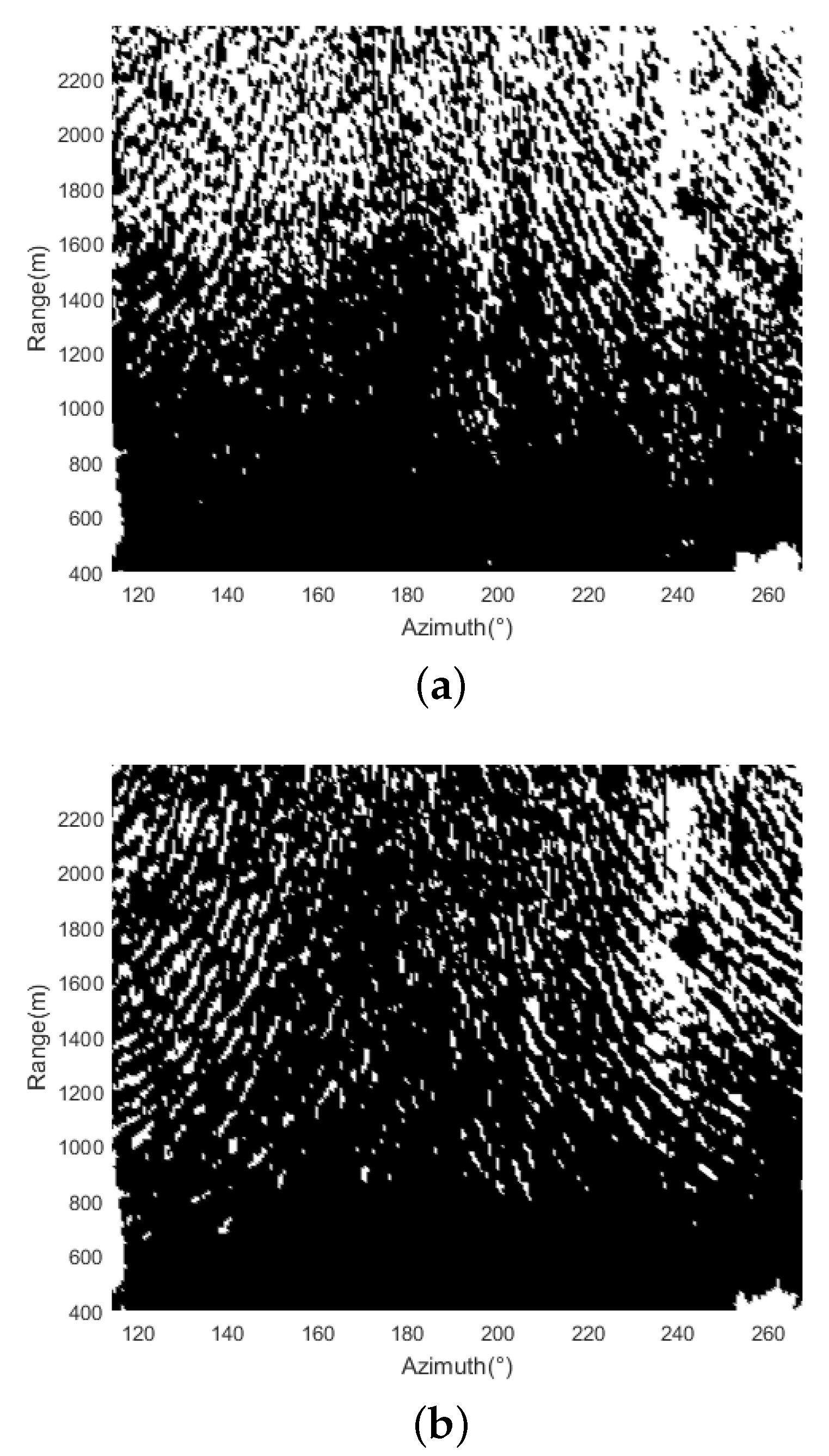
By using the calculated shadow segmentation threshold, the shadow image of the selected analysis area is shown in Figure 7. Figure 7a is the achieved shadow image based on the traditional SSM. Figure 7b is the achieved shadow image obtained by utilizing the proposed adaptive shadow segmentation threshold. The black areas of the shadow image indicate nonshadow areas that can be observed by radar, whereas the white areas indicate shadow areas blocked by front-high waves. In comparison, it can be observed that the shadow areas in Figure 7b are less than those in Figure 7a, especially in the far area of the analysis area selected for the radar platform. The shadow areas near the radar are almost the same since the grazing angle is relatively large, and the sea surface can almost be illuminated by the emitted electromagnetic wave. For the proposed strategy, the attenuation of the echo intensity with distance is appropriately considered. The shadow areas of the analysis areas can be more accurately distinguished. By using the adaptive shadow segmentation threshold, this avoids the bright stripe with a weak echo in the far area being misinterpreted as the shadow area due to the attenuation of the radar echo in the distance.

For the ${180}^{\circ }$ in the azimuth of the radar image, the look direction of the radar is perpendicular to the wave direction. Based on the long peak wave hypothesis, most sea waves can be observed, and the shadow area almost does not exist. From Figure 7b, it can be observed that the area near the ${180}^{\circ }$ in the azimuth is almost the nonshadow area. For the ${270}^{\circ }$ in the azimuth, which is parallel to the wave direction, the estimated shadow areas are similar to those of the traditional SSM.

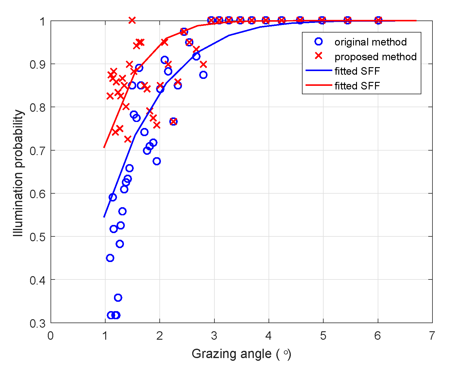
Once the captured shadow image has been segmented into blocks, the shadow ratio function and the illumination ratios in each partition can be obtained. Using the Smith fitting function, the WS for each partition can be calculated with the derived illumination probability. For a partition, the calculated illumination probability and the obtained Smith fitting function as a function of the grazing angle are presented in Figure 8. The horizontal and vertical axes are the grazing angle and the calculated illumination probability. The red cross and the blue circle are the calculated illumination ratio from the shadow images using the traditional and proposed statistical approaches, respectively. The red dashed line and the blue line are fitted with the Smith function, co-ordinated with the probability of illumination. When the adaptive shadow segmentation threshold is used, the illumination probability increases for the low grazing angle compared to that of the traditional shadow threshold. For grazing angles greater than $3^{\circ }$, the obtained illumination probabilities based on the traditional and the adaptive shadow threshold are similar.

When using the traditional SSM with a fixed threshold, the shadow ratio will increase in the distance direction due to the weak backscatter in the distance. Then, the sea surface slope and the SWH will be overestimated [31,32]. However, the estimated sea surface slope decreases when the adaptive shadow threshold is utilized.

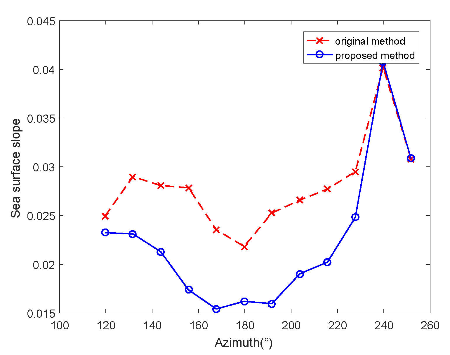
The calculated sea surface slope based on the fixed shadow threshold and the adaptive shadow segmentation threshold in the azimuth is presented in Figure 9. The vertical and horizontal axes represent the obtained RMS sea surface slope and the azimuth, respectively. The red dashed line with the cross indicates the calculated WS based on the traditional hard shadow segmentation method. The blue solid line with the circle is the calculated WS based on the proposed adaptive shadow segmentation threshold. By averaging the WS in each partition, the averaged RMS WS based on the traditional and the proposed SSM can be obtained. It can be observed that the achieved sea surface slope in the azimuth and the averaged RMS based on the adaptive shadow threshold proposed are less than that of the original SSM.

From Figure 9, it can be seen that the WSFV can be constituted by utilizing the obtained sea surface slope in the azimuth. Then, the extracted feature vectors from the dataset are randomly divided into training and test sets, which are utilized to train the model and to verify the retrieving accuracy. Thus, the SWH is calculated by inputting the extracted WSFV of the test set into the SVR model. In order to certify the suitability of the proposed approach, the performance of the adaptive shadow segmentation threshold, the SVR technology, and the constituted feature vector are analyzed below.

Since the wave buoy works for 20 min per hour and outputs one record per hour, the retrieved SWH from the radar data for 20 min is averaged to minimize the error between the buoy records and the SWH extracted from the radar image. The 222 feature vectors are randomly divided into training and test datasets. The training set containing 111 feature vectors is used to achieve the weight and bias parameters. The test set is used to verify the performance of the proposed method. The extracted SNR from the training set is used to obtain the coefficient of the linear relation. Figure 10 is the retrieved SWH based on the radar images and the buoy record. The vertical axis and the horizontal axis represent the SWH and the number of the experimental set, respectively. Since the performance of the different retrieving SWH methods are compared, Figure 10a,b are used to better illuminate the differences in the retrieved SWH based on the test set.

M1 denotes the estimated SWH based on the extracted SNR and the ideal linear relationship to the SNR; M2 is the original SSM, and M3 is the shadow statistical approach using the proposed adaptive shadow segmentation threshold. For M2 and M3, the SWH is estimated based on the relationship of the theoretical derivation to the zero-crossing period and the averaged RMS WS. Instead of using the derivative relationship, the SVR machine learning technology is introduced to calculate the SWH. M4 is the retrieving method based on the SNR and SVR. For M5, the SVR is utilized to achieve the SWH based on the obtained RMS WS compared to M2. For M6, the adaptive shadow segmentation threshold and the SVR are used. Compared to M5 and M6, the constituted feature vector based on the obtained WS in the azimuth is considered in M7 and M8, respectively.

Figure 11 and Figure 12 are the corresponding wind speed and wave direction, respectively. From Figure 12, it can be observed that the domain wave direction is rarely contained in the selected analysis area.

From Figure 10a, it can be observed that the SNR-based method, M1, has the most significant errors compared to the others. Commonly, the SWH increases with increase in the wind speed. Based on the buoy record, it could be observed that the SWH mainly concentrates on the range of 1–2 m. The parameters of the linear relation are determined based on the radar data under low sea conditions. Thus, the M1 algorithm does quite well, except when the wave height is large, such as for samples 15–30 and 75–90. During the period covered by samples 30–40, the retrieving accuracy of the SWH deteriorates, since the wind speed rapidly decays and the wave direction significantly changes. Although the SSM method M2 should have better retrieving accuracy than the spectrum analysis method M1, the performance of the M2 method may be better during the period covered by samples 96–105 since the wind speed decays. By combining the extracted SNR with SVR technology, the retrieving accuracy is greatly improved. When the adaptive segmentation threshold is adopted, the retrieved SWH fluctuates slightly compared to the original SSM. However, the difference is not significant in terms of whether to use the adaptive threshold. From Figure 10b, the retrieving SWH from the radar images fluctuated closely with the buoy record, especially when using the constituted WSFV. The SWH calculated by the proposed method is closest to the wave buoy record. The deviation between the reference and the extracted SWH by using the proposed method is slight.

When the ratio of the training set to the test set is 1:1, the scatterplot between the estimated SWH and the wave buoy record is investigated in detail based on radar Dataset 1, which contains 222 radar image sequences.

Figure 13 is the estimated SWH based on the 3D fast Fourier transform (FFT) spectral analysis method. The horizontal axis and vertical axis indicate the reference value and the retrieved SWH from the radar images, respectively. It can be observed from the point density that the calculated SWH with the 3D FFT approach is mainly concentrated in the range of 0.5∼2.5 m and is lower than the buoy record. The mean bias (BIAS), mean absolute error (MAE), correlation coefficient (CC), and root mean square error (RMSE) are −0.57 m, 0.35 m, 0.57, and 0.73 m, respectively.

The retrieved SWH with the SSM is illuminated in Figure 14. Figure 14a is a scatterplot of the SWH using the original SSM. The BIAS, MAE, CC, and RMSE are −0.34 m, 0.26 m, 0.59, and 0.56 m, respectively. Although the performance is more promising than that of the 3D FFT method, the retrieving accuracy of SWH is not ideal. The point density using the presented adaptive shadow segmentation threshold for the SSM is illustrated in Figure 14b. The BIAS, MAE, CC, and RMSE are −0.38 m, 0.25 m, 0.63, and 0.57 m, respectively. Although the MAE and RMSE are close to that of the original statistical approach, the CC increases by 0.04.

In practice, it is not always possible to retrieve the wave parameters from the shore-based radar images in the sub-area around the upwind direction, which typically has the strongest echo intensity. In this paper, the scatter echo intensity of the shore-based radar images in the downwind direction has to be used to retrieve the SWH due to the influence of the surrounding terrain. Thus, the extracted SWH contains considerable errors based on the 3D FFT and the shadow statistical approaches.

In order to verify the effectiveness of the SVR technology, the performance of the retrieved SWH is presented in Figure 15. Instead of using the linear relationship between the SWH and the SNR, the retrieved SWH based on the SNR and SVR is illuminated in Figure 15a. The BIAS, MAE, CC, and RMSE are −0.09 m, 0.17 m, 0.76, and 0.37 m, respectively. Compared to the traditional 3D FFT approach in Figure 13, the MAE and RMSE decrease by 0.18 m and 0.36 m, respectively. The CC increases by 0.19. The SVR technology can enhance the retrieving precision of the SWH for the SNR feature. A scatterplot of the extracted SWH using the averaged WS and SVR technology is given in Figure 15b. The BIAS, MAE, CC, and RMSE are −0.06 m, 0.22 m, 0.61, and 0.44 m, respectively. Although SVR is adopted, it can be observed that the retrieving accuracy of the SWH is lower than that based on the SNR feature compared to Figure 15a. A scatterplot of the extracted SWH, obtained by utilizing the adaptive shadow segmentation threshold from the SSM and SVR technology, is given in Figure 15c. The BIAS, MAE, CC, and RMSE are −0.11 m, 0.18 m, 0.78, and 0.38 m, respectively. The performance of the extracted SWH is close to that based on the SNR feature. The SVR technology can enhance the extraction accuracy. Compared to Figure 15b, the MAE and RMSE decrease by 0.04 m and 0.06 m, respectively, and the CC increases by 0.17 when the adaptive threshold is used. It is observed that the adaptive shadow segmentation threshold can greatly improve the retrieving accuracy of the SWH when the machine learning technology SVR is used.

Since the echo intensity of the radar image depends on the wind direction, the echo intensity in the downwind and upwind directions approaches the minimum and maximum for the X-band HH polarization radar. Thus, the calculated WS and SWH in the azimuth are different when using the chosen analysis area from the radar images. In order to solve this problem, the WSFV in the azimuth is constituted in this paper. The point density based on the constituted WSFV in the azimuth and the SVR is presented in Figure 16. Figure 16a is the estimated SWH based on the original shadow threshold, the constituted WSFV, and the SVR technology. The BIAS, MAE, CC, and RMSE are −0.04 m, 0.16 m, 0.80, and 0.33 m, respectively. A point density scatterplot of the proposed method utilizing the adaptive shadow segmentation threshold, the constituted WSFV, and SVR is presented in Figure 16b. The BIAS, MAE, CC, and RMSE are −0.03 m, 0.14 m, 0.86, and 0.28 m, respectively. Compared to Figure 16a, it can be observed that the MAE and RMSE are reduced by 0.02 m and 0.05 m, and the CC increases by 0.06. From Figure 16b, the proposed approach in this paper has the best retrieving accuracy from the shore-based radar images compared to the other methods.

Table 1. Comparison of the retrieval results based on radar images from Dataset 1.

Ratio	Index	M1	M2	M3	M4	M5	M6	M7	M8
1:2	BIAS (m)	−0.57	−0.34	−0.36	−0.07	−0.06	−0.07	−0.07	−0.06
	MAE (m)	0.35	0.27	0.26	0.17	0.22	0.18	0.18	0.16
	RMSE (m)	0.72	0.54	0.51	0.35	0.44	0.35	0.34	0.32
	CC	0.53	0.51	0.58	0.75	0.55	0.73	0.74	0.80
1:1	BIAS (m)	−0.57	−0.34	−0.38	−0.09	−0.06	−0.11	−0.04	−0.03
	MAE (m)	0.35	0.26	0.25	0.17	0.22	0.18	0.16	0.14
	RMSE (m)	0.73	0.56	0.57	0.37	0.44	0.38	0.33	0.28
	CC	0.57	0.59	0.63	0.76	0.61	0.78	0.80	0.86
2:1	BIAS (m)	−0.52	−0.35	−0.36	0.01	0.01	−0.07	−0.04	0.02
	MAE (m)	0.32	0.29	0.28	0.17	0.22	0.17	0.16	0.14
	RMSE (m)	0.68	0.56	0.58	0.34	0.40	0.36	0.28	0.26
	CC	0.62	0.64	0.66	0.80	0.73	0.79	0.85	0.89

shows the experimental performance of the retrieved SWH when using radar Dataset 1, collected in January 2015.

Firstly, the performance of the adaptive shadow segmentation threshold is described in detail when the ratio of the training set to the test set is 1:1. When comparing M3 to M2, the CC increases by 0.04. However, the MAE and the RMSE are close. When comparing M6 to M5, it can be observed that the MAE and the RMSE are reduced by 0.04 m and 0.06 m, and the CC increases by 0.17 when the adaptive shadow segmentation threshold is used. When comparing M8 to M7, it can be observed that the MAE and RMSE are reduced by 0.02 m and 0.05 m, and the CC increases by 0.06. Thus, the MAE and RMSE are reduced, and the CC is greatly increased when the adaptive shadow segmentation threshold is used. The adaptive threshold approach can enhance the retrieving accuracy of the SWH for the average wind speed of 5∼10 m/s.

Secondly, the performance of the SVR technology is considered for the shadow statistical approach when the ratio of the training set to the test set is 1:1. When comparing M5 to M2, it can be observed that the MAE and RMSE are reduced by 0.04 m and 0.12 m, and the CC increases by 0.02 when the SVR technology is used. When comparing M6 to M3, it can be observed that the MAE and RMSE are reduced by 0.07 m and 0.19 m, and the CC increases by 0.15 when the SVR technology is used. It is observed that the retrieving accuracy of the SWH is greatly improved when the SVR technology is adopted. The SVR method, which solves different regression problems, considers data errors and model generalization. Therefore, when compared with the original inversion method M2 of the SWH, the SVR-based approach can significantly enhance the inversion accuracy. When compared with M2, M3, and M5, M6 has good performance since both the adaptive shadow segmentation threshold and the SVR technology are introduced into the shadow statistical method.

Finally, the effectiveness of the constituted feature vector based on the obtained WS in the azimuth is certified. When comparing M7 to M5, it can be observed that the MAE and RMSE are reduced by 0.06 m and 0.11 m, and the CC increases by 0.19 when the constituted feature vector is used. When comparing M8 to M6, it can be observed that the MAE and RMSE are reduced by 0.04 m and 0.10 m, and the CC increases by 0.08 when the constituted feature vector is used. During the process of retrieving the SWH, instead of using the averaged RMS WS extracted from the selected analysis area, M7 and M8 have high performance compared to M5 and M6, respectively. Both the MAE and RMSE are reduced, and the CC is increased. The constituted feature vector could solve the problem that the analysis area of the upwind direction could not always be obtained from the radar images for the shore-based marine radar. The experimental results reveal that the inversion accuracy of the SWH is higher, and the error is smaller when the constituted WSFV is used.

In addition, it can be seen from Table 1 that the retrieving accuracy of the SWH increases with increase in the training set. The proposed approach, M8, which uses the adaptive threshold method, constituting the WSFV and SVR technologies, has the highest retrieving accuracy based on the collected shore-based radar data when the proportions of the radar data in the training set to the test set are 1:2 and 1:1. However, the CC and RMSE of M8 is close that of the M7 when the ratio of the training set to the test set is 2:1. With increase in the training set, the effect of the adaptive threshold method is relatively weak since more radar data with a high wind speed are selected as the training set. More radar data under low wind speeds should be utilized to further verify the effectiveness of the adaptive shadow segmentation threshold.

Table 2. Comparison of retrieval results based on radar images from Dataset 2.

Ratio	Index	M1	M2	M3	M4	M5	M6	M7	M8
1:2	BIAS (m)	−0.72	−0.34	−0.38	−0.05	0.05	−0.04	−0.05	−0.07
	MAE (m)	0.42	0.22	0.23	0.18	0.15	0.18	0.15	0.17
	RMSE (m)	0.83	0.46	0.50	0.36	0.30	0.31	0.29	0.35
	CC	0.58	0.80	0.79	0.69	0.80	0.77	0.85	0.81
1:1	BIAS (m)	−0.74	−0.34	−0.39	−0.03	0.04	−0.06	0.04	0.05
	MAE (m)	0.40	0.23	0.23	0.20	0.17	0.19	0.14	0.16
	RMSE (m)	0.83	0.47	0.51	0.37	0.30	0.33	0.25	0.29
	CC	0.56	0.81	0.78	0.71	0.82	0.78	0.88	0.83
2:1	BIAS (m)	−0.77	−0.38	−0.42	−0.06	−0.02	−0.05	−0.05	−0.07
	MAE (m)	0.43	0.22	0.23	0.19	0.16	0.17	0.14	0.15
	RMSE (m)	0.90	0.51	0.55	0.41	0.31	0.34	0.27	0.31
	CC	0.61	0.82	0.81	0.71	0.82	0.80	0.87	0.83

shows the experimental performance of the retrieved SWH when using 258 sets of radar data collected in November 2014. From Table 2, it can be seen that the shadow statistical methods with the combined feature vector and the SVR technology have a relatively high retrieval accuracy. However, the performance of these methods with the adaptive shadow segmentation threshold is a little lower than for the methods without utilizing the adaptive shadow segmentation threshold.

Based on the comparison between M3 and M2 in Table 2, it can be observed that when using the adaptive shadow segmentation threshold, the SWH accuracy is close to that when using the traditional shadow threshold. The traditional shadow method was developed based on geometric optics theory and is suitable for Dataset 2 with high wind speeds. However, under low wind speed conditions, the performance of using an adaptive shadow segmentation threshold strategy is superior to that of using the traditional shadow threshold.

When the ratio of the training set to the test set is 1:1, the retrieved SWH based on the traditional SNR method, M1, has high errors for high wind speeds. However, the performance of M4 significantly improved compared to M1 when the SVR technology was introduced. The BIAS, MAE, and RMSE reduced by 0.71 m, 0.2 m, and 0.46 m, respectively. The CC increased by 0.15.

From Table 2, it can also be seen that the constructed feature vectors can further improve the inversion accuracy of the shadow method under high wind speeds. Compared to M7 and M5, the MAE and RMSE decreased by 0.03 m and 0.05 m, respectively, and the CC increased by 0.06. Meanwhile, the MAE and RMSE decreased by 0.03 m and 0.04 m, respectively, and the CC increased by 0.05 compared to M8 and M6. Thus, this indicates that using the feature vector method can further improve the accuracy of the SWH.

Based on the above analysis, we infer that the effect of the constituted WSFV on improving the retrieval accuracy is dominant. It can be seen that the proposed method with the combined WSFV and SVR technology always improves the CC and decreases the RMSE for both Dataset 1 and Dataset 2.

6. Discussion

Since the scanning period of the radar in this paper is approximately 2.3 s, the retrieved results from the radar images are averaged within 20 min to minimize the measurement error between the marine radar and the wave buoy. Based on the estimated adaptive shadow threshold, the CC of the retrieving SWH from the X-band radar images was improved compared with the original SSM, since the attenuation of the echo intensity of the sea wave in the distance direction was considered for the condition of low wind speeds. Under the condition of low wind speeds, the proposed approach improves the retrieving accuracy of the SWH by using the constructed WSFV with the adaptive shadow segmentation threshold.

The derived SWH from the marine radar images is less than that of the wave buoy under the condition of a high sea. The geometrical optics can provide a good approximation of the typical X-band marine radar, especially when the wind speed increases. Under the condition of a low wind speed, the diffraction is dominant. For the X-band marine radar, the geometrical optics theory is dominant and does not work when the wind speed is greater than 12 m/s and less than 4 m/s, respectively. Geometrical optics and diffraction exist for a wind speed between 4 and 12 m/s. The retrieval accuracy based on Dataset 2 is higher than that based on Dataset 1 since the geometrical optics theory is relatively more applicable.

In this paper, the effect of the wind speed on extracting the SWH is considered. The original SSM can accurately estimate the SWH when the radar data are collected under a wind speed of greater than 15 m/s. However, the SWH is overestimated from the marine radar images when the average wind speed is less than 4 m/s. By investigating in-depth the confidence predictor when using geometrical optics, the geometrical optics theory of shadowing is completely valid when the average wind speed is greater than 12 m/s for the X-band marine radar. However, the geometrical optics theory may work when the average wind speed is 4 ∼12 m/s.

The average wind speed of Dataset 1 is less than that of Dataset 2. The confidence of the geometrical optics increases with increase in the wind speed. For Dataset 2, for a high wind speed, the performance of the adaptive shadow segmentation threshold is close to that of the traditional shadow threshold. However, the performance of using the strategy with the adaptive shadow segmentation threshold under a low wind speed is better than that of using the traditional shadow threshold.

The retrieved SWH based on the proposed SSM is higher than the reference value for the low sea state when the wave height is less than 1 m. Since the echo intensity of the sea clutter is proportional to the sea surface wind, the wind speed and the wind direction should be considered for improving the retrieval performance in the future.

For the SSM, the WS in the azimuth is different because the echo intensity of the sea wave is related to the wave and wind direction. Currently, the influence of the wave direction on retrieving the SWH is rarely considered. During the experiment, it could be observed that the shadow area in Figure 7 and the calculated WS in Figure 9 were related to the wave direction. When the look direction of the radar is parallel to the wave crest, most sea waves can be observed, and the shadow area almost does not exist. In this case, the calculated WS and SWH are underestimated in practice. Therefore, the influence of the wave direction should be considered for further improving the retrieval accuracy of the SWH.

The sea wave is non-uniformly characteristic in the spatial domain for the nearshore area, especially in nearshore areas where the marine environment is influenced by the seabed topography and coastline. Due to the impact of the coastline, the sub-area selected around the upwind direction is not available for retrieving the wave parameters. In these cases, the feature vector is constituted by using the calculated WS in each azimuth partition. The proposed method, which combines the constituted feature vector and the SVR-based technology, exhibits good performance for retrieving the SWH.

Commonly, in practice, vessels may enter the analysis area of interest for the shore-based marine radar. The shadow area is generated by the vessel in the radar look direction since the vessel blocks the propagation direction of the electromagnetic waves. Both the echo intensity of the vessel and the generated shadow area by the vessel are different to that of the sea wave. The influence of vessels increases when more vessels enter the analysis area of interest. Although the proposed method in our manuscript can improve the retrieval accuracy of the SWH under a low wind speed, the influence of the vessel has not been considered. In our experiment, the radar images are manually inspected to eliminate the influence of vessels on retrieving the SWH. When the selected analysis area contains vessels or other objects, the retrieving accuracy of the SWH is reduced for the SSM. Therefore, the influence of vessels should be considered to increase the applicability of the SSM in the future.

7. Conclusions

In order to improve the retrieval accuracy of the SWH from the X-band marine radar images, the SSM, which has the advantage of not requiring external calibration, e.g., from a buoy, is analyzed. Since the echo intensity of sea waves changes dynamically with the distance to the radar platform, an adaptive shadow segmentation threshold that considers the attenuation of the radar echo is proposed to obtain the shadow image. Then, the shadow and nonshadow areas in the original radar image are more reasonably divided. Based on the achieved WSFV with the adaptive shadow segmentation threshold, an approach for extracting the SWH from an X-band marine radar image is presented in this paper. The performance of the retrieved wave height illustrates that the proposed method can enhance the inversion accuracy of the SWH.

Due to the influence of the surrounding terrain and the monsoon characteristics, it is usually impossible to select the analysis area around the upwind direction for retrieving the SWH in the nearshore area. In this paper, the echo intensity difference for the sea clutter in the azimuth is considered. The obtained WS in the azimuth is utilized to constitute the feature vector, which is beneficial for enhancing the retrieving accuracy of the SWH. The sea wave in the nearshore area is commonly nonstationary and nonuniform due to the impact of the complex seabed topography and coastlines. Thus, the classic SVR method is used to calculate the SWH based on the extracted WSFV. The CC between the proposed method and the reference increased by 0.27, and the MAE and RMSE decreased by 0.12 m and 0.28 m, respectively, compared with that of the traditional SSM. The proposed method of retrieving the SWH from marine radar images by using the constituted WSFV and SVR technology can meet the accuracy requirements of engineering.

The wave number and the wave period of the sea wave could be extracted from the radar image sequence based on the traditional spectral analysis method. However, the wave buoy record is used as the ground truth for providing accurate measurement results to reduce the influence of the inaccurate wave period during the retrieval process. Thus, the performance of the SSM is currently evaluated based on the achieved mean zero up-crossing period from the wave buoy. The performance of retrieving the SWH based on the WS and the wave period extracted from radar images should be certified in the future in practice.