Article

Polar Cloud Detection of FengYun-3D Medium Resolution Spectral Imager II Imagery Based on the Radiative Transfer Model

1
Key Laboratory of Infrared System Detection and Imaging Technologies, Shanghai Institute of Technical Physics, Chinese Academy of Sciences, Shanghai 200083, China
2
University of Chinese Academy of Sciences, Beijing 100049, China
3
Zhejiang Lab, Hangzhou 311100, China
*
Author to whom correspondence should be addressed.
Remote Sens. 2023, 15(21), 5221; https://doi.org/10.3390/rs15215221
Submission received: 29 August 2023 / Revised: 22 October 2023 / Accepted: 1 November 2023 / Published: 3 November 2023
(This article belongs to the Special Issue Advances in Remote Sensing and Atmospheric Optics)

Abstract

:
The extensive existence of high-brightness ice and snow underlying surfaces in polar regions presents notable complexities for cloud detection in remote sensing imagery. To elevate the accuracy of cloud detection in polar regions, a novel polar cloud detection algorithm is proposed in this paper. Employing the MOD09 surface reflectance product, we compiled a database of monthly composite surface reflectance in the shortwave infrared bands specific to polar regions. Through the forward simulation of the correlation between the apparent reflectance and surface reflectance across diverse conditions using the 6S (Second Simulation of the Satellite Signal in the Solar Spectrum) radiative transfer model, we established a dynamic cloud detection model for the shortwave infrared channels. In contrast to a machine learning algorithm and the widely used MOD35 cloud product, the algorithm introduced in this study demonstrates enhanced congruence with the authentic cloud distribution within cloud products. It precisely distinguishes between the cloudy and clear-sky pixels, achieving rates surpassing 90% for both, while maintaining an error rate and a missing rate each under 10%. The algorithm yields positive results for cloud detection in polar regions, effectively distinguishing between ice, snow, and clouds. It provides robust support for comprehensive and long-term cloud detection efforts in polar regions.

Graphical Abstract

1. Introduction

The various degrees of cloud cover and shadows that obscure ground information in optical remote sensing images result in blurred and incomplete surface observations, which significantly impact the quality of remote sensing images [1]. Thus, the detection and evaluation of cloud cover in remote sensing images hold great significance, as they form the foundation and key for analyzing and utilizing remote sensing image information.
Cloud detection in remote sensing images represents a prominent research direction in the field of remote sensing image recognition. To tackle cloud detection in remote sensing image recognition, the International Satellite Cloud Climatology Project (ISCCP) was established in 1982, and it was incorporated into the World Climate Research Program [2,3] as a significant component. Since the 1980s, the advancement of remote sensing image processing techniques has led to the gradual development of cloud detection methods with three mainstream approaches: spectral threshold-based, classical machine learning-based, and deep learning-based methods [4]. The spectral threshold-based methods detect clouds by analyzing their spectral characteristics along with those of other targets in the image, employing distinct thresholds across various spectral channels of the remote sensing image [5]. Classical machine learning-based methods employ manually selected image textures, brightness, and other features to train models, such as support vector machines and random forests, enabling the classification of image blocks/pixels and successful cloud detection [6]. Deep learning-based methods utilize a large amount of remote sensing image data to construct deep neural network models that automatically extract data features, yielding cloud detection results of a higher precision [7]. These three mainstream approaches provide various methods and technical avenues for cloud detection in remote sensing images.
However, for clouds and low clouds, especially those covering snow and ice surfaces, the limited disparity in brightness between these clouds and the surface beneath presents multiple challenges in the creation of dependable training data and optical thresholds. In polar regions, clouds and snow frequently demonstrate higher light reflectance and share similar optical characteristics due to the high latitudes, low solar elevation angles, and prolonged presence of extensive ice and snow on the ground, posing significant challenges in cloud detection tasks [8]. Over the past few decades, the severe polar climate and geographical constraints have resulted in a scarcity of ground observation stations. As a result, satellite remote sensing has become the paramount and indispensable approach for cloud observation in the Arctic region. Detecting clouds in polar regions through remote sensing data has persistently posed a complex research challenge.
Cloud and snow detection methods are commonly categorized into spectral thresholding, spatial, and multitemporal approaches [9]. The spectral thresholding method analyzes the spectral band relationships in remote sensing images and utilizes multiple spectral filters to classify clouds and snow. In the spectral thresholding method, the widely employed index for generating a snow mask is the Normalized Difference Snow Index (NDSI) [10]. Zhu et al. proposed [3] the Tmask algorithm for cloud, cloud shadow, and snow detection in Landsat satellite images, which identifies snow pixels by applying thresholds to multiple spectral bands.
Spatial methods commonly rely on statistical and deep learning models. Chen et al. introduced [11] a cloud and snow detection algorithm that utilizes a support vector machine (SVM). The SVM, a supervised machine learning algorithm, is primarily employed for tasks related to classification and regression. The SVM endeavors to discover an optimal hyperplane or decision boundary within a high-dimensional space, effectively separating data points into distinct classes or predicting numeric values. It accomplishes this by maximizing the margin between the classes, where the support vectors represent data points nearest to the decision boundary [12]. Since clouds and ice and snow surfaces are difficult to distinguish in Antarctic areas, accurate training samples are hard to obtain. But the SVM has an advantage to solve this problem of limited samples with the hyperplane theory. Moreover, it can be extended from the linear classifier to the nonlinear classifier, with classification suitable for from two classes to multiple classes. The method employs the Gray Level Co-occurrence Matrix (GLCM) algorithm to extract five distinct texture features from cloud and snow regions, followed by the utilization of a nonlinear support vector machine to determine the optimal classification hyperplane using training data for cloud and snow detection. Zhan et al. developed [8] a pixel-level fully convolutional neural network for detecting clouds and snow. This method introduces a specially designed fully convolutional network to capture cloud and snow patterns in remote sensing images, incorporating a multiscale strategy for fusing low-level spatial information and high-level semantic information. Finally, the algorithm is trained and evaluated using manually annotated cloud and snow datasets.
Multitemporal methods differentiate between clouds and snow by utilizing multiple images collected at the same location but at different times. Bian et al. proposed a practical multitemporal cloud and snow detection method that combines spectral reflectance with spatiotemporal background information. Multitemporal methods for discriminating clouds and snow often employ the NDSI to extract snow pixels [13]. However, these methods are unsuitable for scenarios with insufficient multitemporal remote sensing images as input.
Spectral thresholding currently serves as the mainstream method for cloud and snow detection. However, its single threshold approach exhibits low accuracy and faces challenges in effectively distinguishing between clouds and snow in polar regions. This paper’s objective is to enhance cloud detection accuracy over the ice- and snow-covered surfaces of polar regions. Accordingly, we introduce a novel, computationally efficient, physically simulated method for cloud detection in polar regions. Initially, we compiled a database of the true surface reflectance in polar regions under clear-sky conditions, utilizing MODIS’s 8-day composite surface reflectance product (MOD09A1). We subsequently employed the 6S model (Second Simulation of a Satellite Signal in the Solar Spectrum) for forward simulation, acquiring the apparent reflectance of the corresponding pixel under clear-sky conditions. By comparing this simulated apparent reflectance with the actual value, we ascertained the presence of clouds in that pixel. This method, with its efficient computational capabilities, adeptly tackles the intricate challenge of cloud detection over polar ice and snow surfaces. It robustly supports comprehensive, long-term cloud detection initiatives in polar regions and bolsters research on Arctic navigation routes and sea ice observation.

2. Study Area and Data

2.1. Study Area

The polar regions serve as the Earth’s primary sources of cold and represent crucial and sensitive areas for global change [14]. They play a critical role in regulating the global energy balance, water balance, and temperature–salinity balance. The polar regions experience high cloud coverage year-round, with average cloud amounts of approximately 0.4 during winter and spring and around 0.7 during summer and autumn. Owing to the intricate polar weather conditions and the prevalence of ice and snow surfaces, there exist minimal radiation distinctions between clouds and the underlying ice and snow surfaces in both visible and thermal infrared channels. This can potentially result in the misidentification of clouds and ice/snow regions.
This study focused on the Arctic region located north of 66.34° latitude and the Antarctic region located south of 66.5° latitude as the study areas, as shown in Figure 1. It proposed a cloud detection method tailored specifically for polar ice and snow surfaces.

2.2. FY-3D MERSI-II Imagery

China’s second-generation polar-orbiting meteorological satellite, the Fengyun-3 (FY-3), operates at an orbital height of 836 km and completes a repeat cycle every 5.5 days. Its objective is to conduct all-weather, multispectral, three-dimensional observations of global atmospheric and geophysical elements. Its primary function is to provide satellite observational data for medium-range numerical weather prediction and to monitor ecological environments and large-scale natural disasters. Additionally, it offers satellite meteorological information for global environmental change research, global climate change research, and diverse sectors, including oceanography, agriculture, forestry, aviation, and the military.
In this study, data were acquired using the Medium Resolution Spectral Imager II (MERSI-II) sensor, which captured images of the same target one to two times daily. Covering a strip area of 2900 km, the MERSI-II sensor captures images across the orbital direction, ranging from −55.04° to 55.04°, using a 45° scan mirror [15]. The Medium Resolution Spectral Imager II (MERSI-II) is equipped with a total of 25 channels, comprising 16 visible near-infrared channels, 3 shortwave infrared channels, and 6 medium-longwave infrared channels. Out of these channels, 6 have a ground resolution of 250 m, whereas the remaining 19 have a ground resolution of 1000 m, as detailed in Table 1. Files are partitioned and distributed at 5 min intervals in a hierarchical data format (HDF5), resulting in a granule size of 2000 rows × 2048 columns in the 1 km resolution product (1000M_MS). The 1 km resolution file includes the visible (0.470 to 0.865 μ m) and TIR (10.8 and 12.0 μ m) bands aggregated to 1 km from the original 250 m resolution, while the other 19 channels maintain the original sampling resolution of 1 km. Additionally, a separate geolocation file (GEO1K) is provided, containing latitude and longitude information for each pixel, along with sun and sensor zenith and azimuthal angles, a land/water mask, and a Digital Elevation Model (DEM). FY-3D data can be accessed from the National Satellite Meteorological Centre of China at http://satellite.nsmc.org.cn/PortalSite/Data/DataView.aspx?currentculture=zh-CN (accessed on 3 March 2023). MERSI-II’s primary objective is to dynamically monitor Earth’s environmental elements, including its oceans, land, and atmosphere. It particularly focuses on crucial atmospheric and environmental parameters, such as cloud characteristics, aerosols, land surface properties, ocean surface properties, and the lower tropospheric water vapor. The operational presence of MERSI-II in orbit enhances satellite remote sensing observations in fields like weather forecasting, climate change research, and Earth environmental monitoring.

2.3. MODIS Surface Reflectance Products

The MODIS (Moderate Resolution Imaging Spectroradiometer) is a medium-resolution imaging spectroradiometer mounted on the Terra and Aqua satellites, enabling a complete scan of the Earth’s surface every one to two days. The instrument comprises 36 spectral bands covering the visible and infrared spectrum range (0.4–14.4 μ m), offering spatial resolutions ranging from 250 m to 1000 m. It provides extensive global data on cloud cover, radiative energy, and changes in oceans and land [16].
Data from MOD09, a Level 2 land surface reflectance product provided by MODIS, are derived from calculations based on MOD02 data. The data are provided in seven bands: the first band (620–670 nm), second band (841–876 nm), third band (459–479 nm), fourth band (545–565 nm), fifth band (1230–1250 nm), sixth band (1628–1652 nm), and seventh band (2105–2155 nm), at a spatial resolution of 500 m. This product estimates the land surface reflectance for each band without atmospheric scattering or absorption. It also corrects for atmospheric and aerosol effects, serving as the foundation for generating higher-level gridded level-2 data (L2G) and level-3 data. The MOD09 series consists of various products, including Level 2 (MOD09), Level 2G (MOD09GHK, MOD09GQK, MOD09GST), Level 2G-Lite daily (MOD09GA, MOD09GQ), Level 3, 8-day composited (MOD09A1, MOD09Q1), and daily Level 3 CMG (MOD09CMG, MOD09CMA) products, as shown in Table 2 [17].
The MOD09A1 product offers land surface reflectance data and quality assessment for MODIS bands 1–7. This product is a Level 3 product synthesized from MOD09GA data, featuring a spatial resolution of 500 m. It utilizes a sinusoidal projection and incorporates exclusively daytime land surface reflectance data. During production, this product considers factors such as aerosol, atmospheric scattering and absorption, changes in land cover types, bidirectional reflectance distribution function (BRDF), atmospheric coupling effects, and thin cloud contamination. It is derived by atmospherically correcting MODIS Level 1B data, achieving an overall accuracy of ±(0.005 + 0.05 × ρ ). Each pixel is acquired within an 8-day period using maximum probability L2G observations. These observations consider a wide range and low viewing angles, excluding the effects of clouds, cloud shadows, and aerosols. Table 3 provides the parameters and theoretical accuracy of each band in MOD09A1. It shows that the absolute errors of each band are small (<0.015), and the relative errors, except for the third band, are also small. This indicates that the product has excellent estimation capabilities for land surface spectral reflectance in different bands [18].

2.4. MODIS Cloud Mask Products

MOD35 is a Level 2 cloud mask product with a 1 km resolution provided by NASA MODIS. To achieve precise cloud identification, the MODIS cloud mask algorithm utilizes a series of spectral tests based on methodologies used in the AVHRR Processing scheme Over cLoudy Land and Ocean (APOLLO), International Satellite Cloud Climatology Project (ISCCP), Cloud Advanced Very High Resolution Radiometer (CLAVR), and Support of Environmental Requirements for Cloud Analysis and Archive (SERCAA) algorithms to identify cloudy fields of views (FOVs). Based on these tests, each FOV is assigned a clear-sky confidence level (high confidence clear, probably clear, undecided, cloudy). In case of inconclusive results, spatial- and temporal-variability tests are conducted. The spectral tests utilize radiance (temperature) thresholds in the infrared and reflectance thresholds in the visible and near-infrared. Thresholds depend on factors such as the surface type, atmospheric conditions (moisture, aerosol, etc.), and viewing geometry. Inputs for the algorithm include MOD02 calibrated radiances, a 1 km land/water mask, DEM, ecosystem analysis, snow/ice cover maps, National Centers for Environmental Prediction (NCEP) analysis of surface temperature and wind speed, and an estimation of precipitable water [19,20].

2.5. Aerosol Robotic Network (AERONET)

The ground-based observation data used in this study were obtained from the AERONET observation network (https://aeronet.gsfc.nasa.gov/, accessed on 8 March 2023). AERONET, along with other aerosol observation networks worldwide, including the French aerosol network (PHOTONS) and some research institutions, constitutes a ground-based aerosol observation network alliance. AERONET employs the CE-318 sun photometer to measure the radiation intensity in different spectral bands of direct solar radiation and to calculate the aerosol optical thickness in the atmospheric column. It records various measurement values every 15 min or at shorter intervals, ensuring low uncertainty. AERONET offers high-precision and standardized data products for all sites, and its aerosol observation data have been extensively utilized in validating satellite sensor Aerosol Optical Depth (AOD) products. AERONET offers three levels of data products: Levels 1.0, 1.5, and 2.0. Level 1.0 does not undergo cloud filtering and quality checks, Level 1.5 undergoes cloud filtering without quality verification, and Level 2.0 is a high-precision data product that has undergone rigorous cloud filtering, manual verification, and quality assurance [21]. Currently, AERONET operates more than 500 sites globally, approximately 40 of which are located in polar regions, as depicted in Figure 2. This study concentrates on the polar regions, thus selecting data from sites distributed in the Arctic and Antarctic.

3. Methods

3.1. Theoretical Foundation

In the shorter wavelength range of visible light, the reflectance between clouds and ice/snow exhibits minimal differenceS. Traditional threshold-based methods, like ISCCP, APLOLLP, and CLAVR, fail to detect clouds and ice/snow effectively through the use of suitable thresholds. The near-infrared and shortwave infrared bands exhibit differences in reflectance between clouds and ice/snow, enabling the separation of cloud layers and ice/snow, thereby enhancing cloud detection accuracy. Figure 3 shows the spectral reflectance curves of ice/snow, which were collected from the ASTER spectral library [22]. Moreover, the spectra of clouds were collected from the Airborne Visible Infrared Imaging Spectrometer, a hyperspectral data sensor with 224 spectral bands covering a spectral range of 0.4–2.5 μ m with a spectral resolution of 10 nm.
However, remote sensing images typically consist of a significant number of mixed pixels. Each pixel in satellite imagery covers a large area due to the sensor’s low spatial resolution, resulting in the inclusion of multiple types of land cover information [23]. In polar regions, cloud pixels in remote sensing images are typically obscured by thin or broken clouds, leading to the reflectance of pixels in polar regions being influenced by the combined interactions of clouds and ice/snow. Broken clouds often manifest as small, isolated patches, covering a limited section of the cloud. Substantial gaps exist between these cloud patches, rendering them notably distinct at the image’s edges. Thin clouds are typically characterized by their relatively low thickness, permitting the passage of some light through the cloud layer, generally within the optical thickness range of 0.1 to 3. In the shortwave infrared band, the reflectance of thin or fragmented clouds closely resembles that of the underlying ice/snow in polar regions. Mixed pixels composed of clouds (especially thin clouds, fragmented clouds, and cloud edges) and underlying ice/snow surfaces exhibit the phenomenon of “same spectrum, different objects” or “same objects, different spectra”, which significantly impacts cloud detection accuracy in polar regions. The reflectance of mixed pixels can be expressed as a linear combination of the constituent component’s reflectance and the ratio of their pixel areas [24].
P = i = 1 N c i e i + n = E c + n
i = 1 N c i = 1
Here, N represents the total number of pixels, P represents the reflectance of the mixed pixel, E is an m × n matrix, e i represents the proportion of each component, c i represents the area proportion of e i in P, and n represents uncertainty.

3.2. Construction of Polar Cloud Detection Model

3.2.1. Polar Surface Reflectance Database Construction

The 1.64 μ m band of MOD09A1 data is selected, followed by batch geometric correction of the filtered data, and, finally, the mosaicking process is conducted in the North and South Poles. The projection and coordinate systems of the surface reflectance data are unified to the Universal Polar Stereographic Projection (UPS) and WGS84 coordinate system during the geometric correction process in this study.
It is assumed that the surface reflectance of most land cover remains relatively constant over a specific period [21]. Based on this assumption, monthly compositing of MODO9A1 data was performed to create a database of monthly composited surface reflectance for cloud detection purposes. To effectively enhance the utilization of image data, ensure spatial continuity in surface reflectance, and preserve spectral information accuracy, additional processing of the four MODO9A1 datasets within each month is necessary. By removing clouds, cloud shadows, and outliers, the original information of the data is preserved to the maximum extent. Since clouds, cloud shadows, and outliers in the images frequently result in substantial variations in reflectance values, we chose the second smallest value among the four datasets for each pixel as the composited monthly surface reflectance value to build a database of surface reflectance for the North and South Poles. Figure 4 displays the composited surface reflectance data for the North and South Poles in June 2022 at a single channel of 1.64 μ m, illustrating the strong spatial continuity of the data.

3.2.2. 6S Model Forward Simulation

The 6S model was developed in 1997 by Vermote et al. from the Department of Geography at the University of Maryland, USA, as an extension of the 5S model. The primary aim of the 6S model is to simulate the radiance received by a sensor under cloud-free conditions while accounting for the absorption and scattering effects of atmospheric components on solar radiation under non-Lambertian surfaces. It is applicable across the wavelength range of 200 nm to 4000 nm. In contrast to the 5S model, the 6S model incorporates factors such as the target height, non-Lambertian surfaces, and the influence of additional absorbing gases, like CH 4 , N 2 O, CO, and others. The successive order of scattering (SOS) algorithm is employed to calculate the scattering and absorption effects, thereby improving the accuracy of the model [25,26]. In the 6S model, the first step is the direct radiation of sunlight passing through aerosols and directly illuminating the target object. Secondly, as a result of aerosol scattering, light that originally could not directly illuminate the target becomes indirectly illuminated upon scattering. The 6S model employs a concept similar to transmittance to quantify the magnitude of this light component. Additionally, during the upward transmission of reflected light from the surface target, some light is scattered back and illuminates the surface target again, owing to the backscattering effect of aerosols [26]. This process encompasses the irradiance received by the surface, as illustrated below.
E s o l = μ s E s ( e τ / μ s + t d ( θ s ) ) ( ρ t S + ρ t 2 S 2 + ) = μ s E s ( e τ / μ s + t d ( θ s ) ) 1 ρ t S
μ s = cos ( θ s ) represents the cosine of the solar zenith angle, E s represents the solar irradiance at the top of the atmosphere, and t denotes the aerosol optical thickness in the vertical direction. t d ( θ s ) represents the diffuse transmittance coefficient, which measures the magnitude of the diffuse radiation transmitted through the aerosol layer and illuminating the surface target due to aerosol scattering. p represents the reflectance of the surface target, and S represents the spherical albedo of the atmosphere, indicating the magnitude of the backscattered reflection of the surface object when it passes through aerosols.
The aforementioned phenomenon is a result of the presence of aerosols, which induce variations in the irradiance received by surface objects. Furthermore, the presence of aerosols also leads to the composition of the radiation received by the sensor being divided into three distinct parts.
First, the reflected light from the surface object reaches the sensor directly after passing through aerosols.
E r e d i r = E s o l ρ t e τ / μ v
μ ν = cos ( θ ν ) represents the cosine of the sensor zenith angle. Secondly, when sunlight illuminates aerosols, some of the light is scattered backward by the aerosols and does not reach the ground. Instead, it goes directly back to space, and a portion of it enters the sensor.
E r e d i f f = E s ρ a ( θ s , θ ν , φ s φ ν )
Lastly, the scattering effect of aerosols causes a portion of the reflected light from surrounding objects to enter the optical path of the target. When the target and the surrounding objects belong to the same category, this portion of light enhances the target’s radiation and is deemed a useful component. However, if the target and the surrounding objects differ in category, this portion of light introduces additional environmental interference known as the adjacency effect.
E r e c r o s s = E s o l ρ e ( M ) t d ( θ v )
Therefore, the total radiation received by the sensor is
E r e = E r e d i f f + E r e d i r + E r e c r o s s = μ s E s ρ a ( θ s , θ ν , φ s φ ν ) + μ s E s ( e τ / μ s + t d ( θ s ) ) 1 ρ S ( ρ i e τ / μ i + ρ e ( M ) t d ( θ ν ) )
By employing the aforementioned model to simulate the apparent reflectance based on surface reflectance, highly accurate results can be achieved.
The inputs for the 6S model primarily consist of the observation geometry, atmospheric model, aerosol model, aerosol optical thickness, surface reflectance, and sensor spectral characteristics. The observation geometry encompasses the solar zenith angle, solar azimuth angle, satellite zenith angle, and satellite azimuth angle, which are stored in the geolocation file of FY-3D MERSI-II data.
In practical simulations, considering the climatic characteristics of the polar regions, we configure the atmospheric model as either subarctic summer or subarctic winter, depending on the specific conditions. For the Arctic, we employ the maritime-type aerosol model, while for the Antarctic the continental-type aerosol model is used. The aerosol optical thickness is derived from the AOD data product obtained through the AERONET observation network at Arctic sites. However, as the 6S model necessitates aerosol optical thickness input at 550 nm and AERONET provides AOD measurements only at wavelength channels of 340, 380, 440, 500, 670, 870, and 1020 nm, we employ a quadratic polynomial interpolation method to interpolate the known AOD values from AERONET channels to 550 nm. The process of obtaining the AOD at the AERONET 550 nm channel using quadratic polynomial interpolation is as follows:
l n τ = 0 + 1 l n λ + 2 ( λ ) 2
where τ represents the AOD value at the channel and i ( i = 0 , 1 , 2 ) are unknown coefficients that can be estimated using the least squares method in combination with the known AOD values from AERONET channels.
Regarding the sensor’s spectral characteristics, we integrate the spectral response function of the 1.64 μ m channel from FY-3D MERSI-II (refer to Figure 5) into the 6S model. This incorporation of the spectral response function enables accurate modeling and analysis within the 6S framework.

3.2.3. Cloud Detection Model

Before constructing the cloud detection model, preprocessing is necessary for the 1.64 μ m channel data from FY-3D MERSI-II. The first step involves restoring and adjusting the D N (Digital Number) values of the channel.
D N * * = S × D N * I
In the equation, D N * * represents the restored results, D N * corresponds to the count values in the scientific dataset EV of the LI data, and S and I are adjustment coefficients that can be obtained by querying the internal properties of EV.
Subsequently, the channel undergoes radiometric calibration based on the DN. This is followed by a quadratic calibration process, resulting in the calibrated apparent reflectance.
ρ * = k 0 + k 1 × D N * * + k 2 × D N * * 2 × d E S 2 / cos θ
In the equation, the symbol ρ * represents the calibrated reflectance. Additionally, θ denotes the solar zenith angle; d E S represents the square of the Earth–sun distance; and k 0 , k 1 , and k 2 are the calibration coefficients. These calibration coefficients can be obtained by querying the “VIS_Cal_Coeff” attribute in the scientific dataset EV.
The cloud detection principle in this study involves simulating the complete range of apparent reflectance variations using the 6S model. This simulation corresponds to the actual surface reflectance under different observation and atmospheric conditions. If the measured apparent reflectance of a pixel from the image surpasses the maximum simulated value, the pixel is classified as cloud-contaminated. Otherwise, it is classified as clear-sky. The solar and satellite zenith angles cover all possible values for the satellite sensor employed in this study. The proposed polar cloud detection model for FY-3D MERSI-II data is as follows:
ρ N o r t h P o l a r * = 0.539187 · ρ N o r t h P o l a r 0.002571 · cos α cos β + 0.101877
ρ S o u t h P o l a r * = 0.668803 · ρ S o u t h P o l a r 0.002951 · cos α cos β + 0.080149
R = ρ * ρ *
The equations includes ρ * , which signifies the maximum value of the simulated apparent reflectance variations under diverse conditions. ρ denotes the surface reflectance sourced from the database. α stands for the solar zenith angle, β represents the satellite zenith angle, ρ * represents the apparent reflectance extracted from the remote sensing image, and R signifies the ultimate cloud detection outcome. Limited by the 1.64 μ m band characteristics, this method can only work in the daytime and is not suitable for night. Therefore, when the algorithm is applied to the polar region, it is important to check whether the image is in daytime. Figure 6 shows the flowchart of the proposed algorithm.

3.2.4. Evaluation Methods

To quantitatively assess the effectiveness of cloud detection algorithms and the accuracy of the results, this study employs remote sensing visual interpretation to extract actual cloud content information from the images and perform accuracy verification. The MERSI-II data’s 0.47 μ m, 1.61 μ m, and 2.1 μ m bands are assigned to the R, G, and B channels, respectively, for false-color synthesis, which is widely used for cloud and snow display. Using ArcGIS 10.8 software, the original cloud-sensitive 1.64 μ m single-channel image and the false-color synthesized image mentioned above are compared, and cloud information is extracted by manually selecting features to generate a cloud mask product. This cloud mask product is used to validate the real cloud coverage data of the cloud detection results in this study, ensuring the accuracy of the results. Figure 7 displays various types of clouds, including partial fragmented clouds and thick clouds, as observed in the remote sensing visual interpretation results.
In addition, we select a coarse-to-fine unsupervised machine learning algorithm (CTFUM) for comparative verification [27]. CTFUM is an improved machine learning method, which extracts color, texture, and statistical features of remote sensing images using color transformation, dark channel estimation, Gabor filtering, and local statistical analysis. Then, an initial cloud detection map can be obtained by using the support vector machines (SVMs) on the stacked features, in which the SVM is trained with a set of samples automatically labeled by processing the dark channel of the original image with several thresholding and morphological operations. Finally, guided filtering is used to refine the boundaries in the initial detection map.
In Table 4, T P represents the number of pixels identified as cloud in both the cloud detection result and the actual cloud result; F N represents the total number of pixels identified as clear-sky in the cloud detection result but as cloud in the actual cloud result; T N represents the total number of pixels identified as clear-sky in both the cloud detection result and the actual cloud result; and F P represents the total number of pixels identified as cloud in the cloud detection result but as clear-sky in the actual cloud result [28].
The cloud amount ( C A ) index was chosen to represent the overall cloud content in the remote sensing image, while the cloud amount error ( C A E ) indicates the disparity between the detected cloud amount and the actual cloud distribution [29]. A positive C A E value suggests an overestimation of the clouds in the image, with a larger value indicating a more pronounced misjudgment. Conversely, a negative C A E value indicates an underestimation of clouds, and a smaller value signifies a more significant missed detection. Four typical evaluation metrics, namely a c c u r a c y , p r e c i s i o n , r e c a l l , and the F1 score, are chosen to quantitatively assess the cloud detection results at each pixel. These metrics offer different perspectives for evaluating the model’s performance in classification tasks. Accuracy is a straightforward metric that represents the ratio of correctly classified samples to the total number of samples. It provides an overall measure of the classification correctness and is suitable when the dataset has a balanced class distribution. However, accuracy can be misleading in the presence of class imbalance. Precision refers to the proportion of true positives among all samples predicted as positive. It focuses on the model’s accuracy in predicting positive samples and indicates the “precision rate” of the model. In other words, it measures how many predicted positive samples are actually true positives. A high precision signifies a low false positive rate in predicting positive samples. Recall, in contrast, represents the proportion of true positives among all actual positive samples. It assesses the model’s ability to capture true positive samples and corresponds to the “recall rate” of the model. In simple terms, recall measures how many true positive samples the model can correctly predict. A high recall indicates a low false negative rate in capturing positive samples. The F 1 score is the harmonic mean of precision and recall. It offers a comprehensive evaluation by considering the balance between precision and recall. A high F 1 score indicates a favorable trade-off between precision and recall, suggesting a well-balanced performance of the model [30].
C A = N c l o u d N
C A E = C A p r o d u c t C A r e a l
A c c u r a c y = T P + T N T P + T N + F P + F N
P r e c i s i o n = T P T P + F P
R e c a l l = T P T P + F N
F 1 = 2 P r e c i s i o n R e c a l l P r e c i s i o n + R e c a l l
In the equations, N c l o u d represents the total number of cloud pixels in the image; N represents the total number of pixels in the image; and C A p r o d u c t and C A r e a l represent the cloud amount in the cloud detection result and the actual cloud result (i.e., the results of visual interpretation in remote sensing).

4. Results

4.1. Dataset and Experimental Setup

We primarily evaluate the performance of the proposed cloud detection method using FY-3D MERSI-II remote sensing images. The multispectral images are reprojected into UPS at a spatial resolution of 1000 m. The validation images, collected from 2020 to 2022 in the polar regions, cover an area of 400,000 × 400,000 m and encompass clouds of various forms and thicknesses over ice and snow surfaces. We compare the 1.64 μ m single-channel image and the false-color synthesized image used in this study through remote sensing visual interpretation to extract cloud information and verify its accuracy against real cloud results.
We select a total of 100 sub-images from the FY-3D MERSI-II remote sensing images for cloud detection experiments and validation. The performance of the proposed cloud detection algorithm is then compared with the MOD35 cloud product on these sub-images. Table 5 shows the acquisition time and range of each piece of data.

4.2. Comparative Analysis of Proposed Algorithm with Machine Learning Algorithms and MOD35

Figure 8, Figure 9 and 
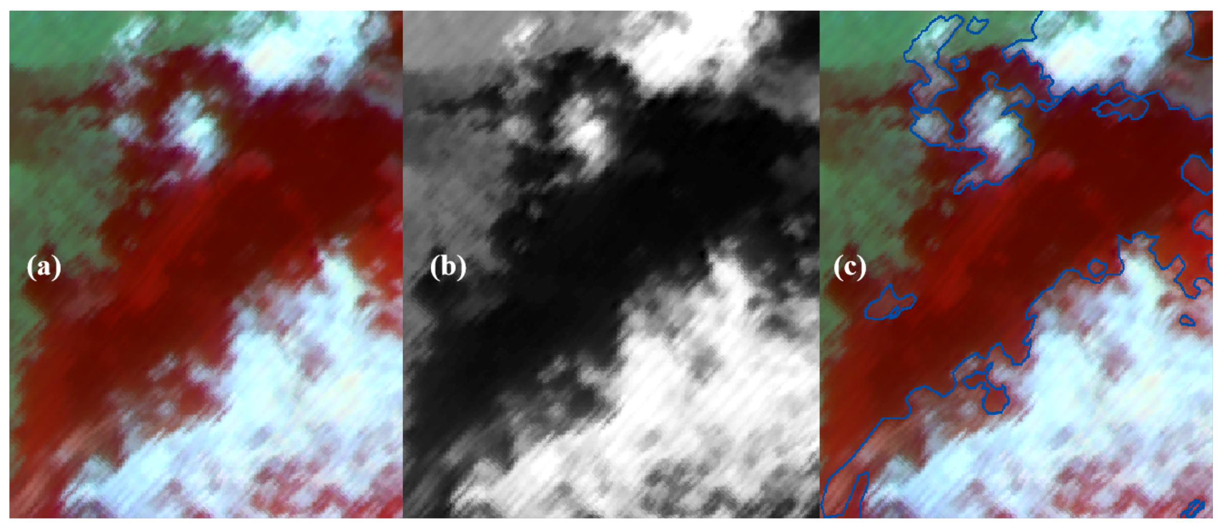
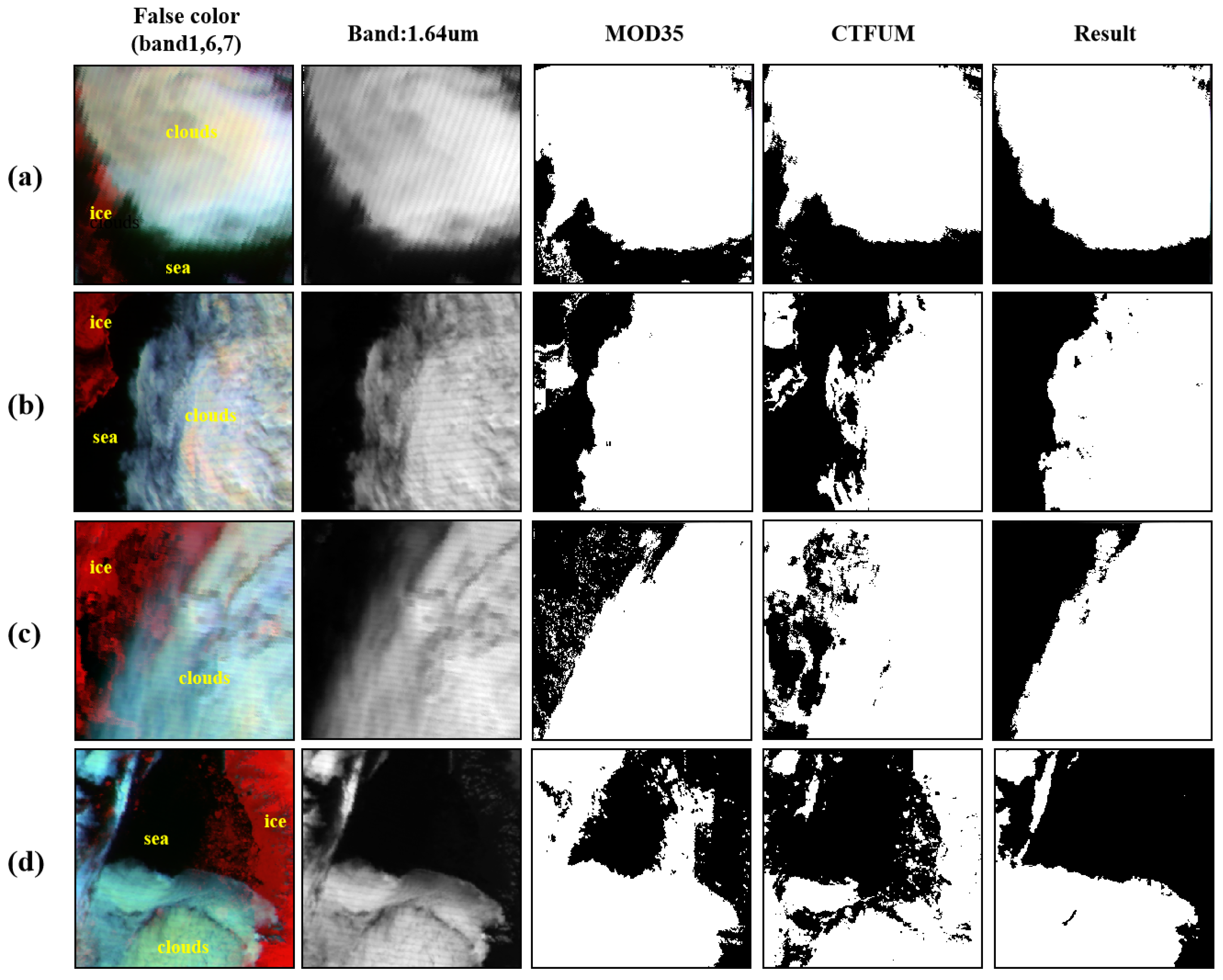
Figure 10 showcase the comparative analysis between the cloud results of the proposed algorithm in this paper with CTFUM and the cloud mask products provided by MODIS, encompassing various cloud types across distinct regions. The first column of the figures displays the pseudo-color composite image of the MERSI-II 1.6.7 band (representing 0.47 μ m, 1.64 μ m, and 2.13 μ m), while the second column exhibits the 1.64 μ m single-channel image, which is specifically responsive to clouds and utilized for aiding cloud identification purposes. The third column illustrates the MODIS cloud product MOD35, while the fourth column portrays the cloud detection results of CTFUM. The last column shows the cloud product generated through the cloud detection algorithm proposed within this paper.
Figure 8 shows the comparison of the proposed cloud detection algorithm with CTFUM and MOD35, specifically in their ability to differentiate between fractured polar sea ice and clouds. It is evident from the figure that MOD35 and CTFUM frequently confuse sea ice with clouds, erroneously identifying fragmented sea ice within seawater as cloud pixels. The elevated cloud content C A p r o d u c t of MOD35, relative to the authentic cloud content C A r e a l , further signifies the incorrect identification of fractured sea ice by MOD35. Importantly, in Figure 8c, both MOD35 and the outcomes of this paper (even though MOD35 incorrectly identifies some sea ice) indicate underestimated cloud extents, with both algorithms being unsuccessful in accurately detecting exceedingly thin clouds at the cloud peripheries. Overall, the outcomes of this paper surpass those of MOD35 and CTFUM concerning a c c u r a c y , p r e c i s i o n , r e c a l l , and F1 score. This is primarily evident in the superior accuracy of identifying fractured sea ice and clouds within the outcomes of this paper while successfully avoiding the misidentification of sea ice as clouds. Specifically in Figure 8d, the a c c u r a c y , p r e c i s i o n and F1 of MOD35 are 84.94%, 75.63%, and 86.05%, respectively, and those of CTFUM are 84.10%, 78.73%, and 84.44%, whereas the outcomes of this paper display remarkable enhancement over MOD35 and CTFUM in these three metrics, achieving 98.94%, 97.57%, and 98.73%, respectively.
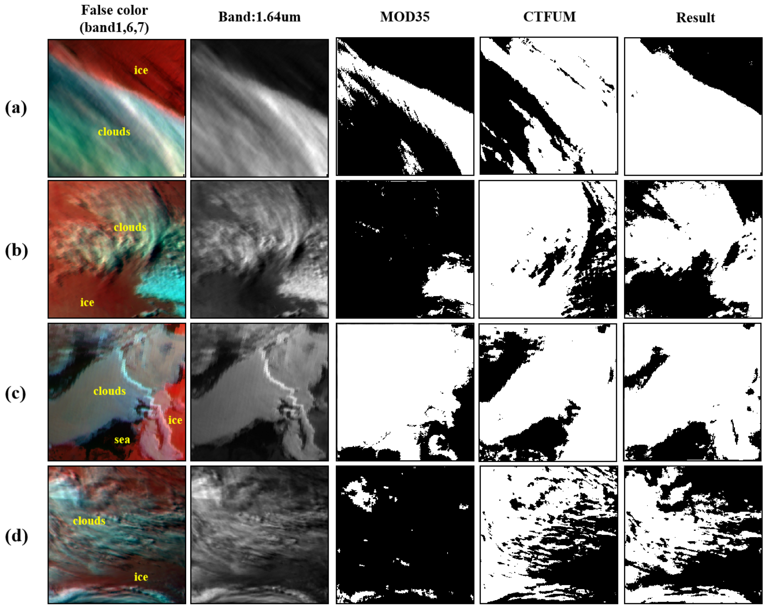
Figure 9 illustrates the outcomes of the proposed cloud detection algorithm, CTFUM, and MOD35 in their capability to identify polar thick clouds. Figure 9a,b,d provide intuitive evidence that the MOD35 cloud product notably overlooks the identification of thick clouds in the atmosphere above polar ice and snow surfaces. These instances yield r e c a l l values of merely 43.07%, 16.1%, and 6.65%, along with a c c u r a c y values of 62.41%, 48.07%, and 27.41%, correspondingly. CTFUM misidentifies a large amount of snow and ice as clouds, and the ability to identify cloud edges is not strong. The cloud detection algorithm advocated in this paper adeptly discerns the majority of thick clouds situated above polar ice and snow, attaining a r e c a l l surpassing 97% while consistently upholding an a c c u r a c y exceeding 95%. Furthermore, the outcome depicted in Figure 9c indicates that when thick clouds emerge above polar seawater MOD35 inaccurately identifies the seawater as clouds, which also occurs in UFTUM, consequently overestimating cloud presence. Nonetheless, the algorithm put forward in this paper rectifies MOD35’s and UFTUM’s misidentification, effectively achieving precise differentiation between seawater and clouds.
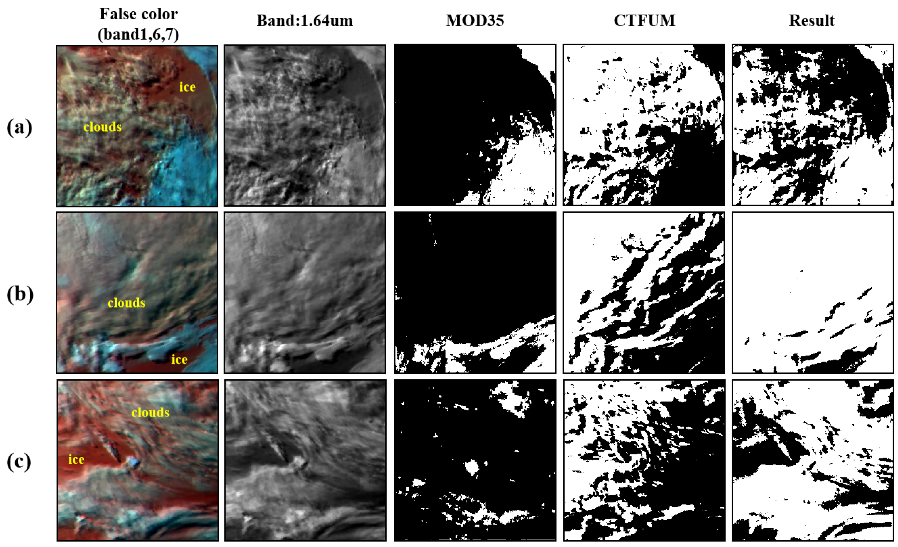
Figure 10 displays the outcomes of the proposed cloud detection algorithm, CTFUM, and MOD35 in identifying polar thin and fragmented clouds. Among them, Figure 10a,c reveal that in identifying fragmented clouds within the polar ice and snow-covered region MOD35 exhibits limited detection capability and notable omissions, yielding a c c u r a c y , r e c a l l , and F1 score values all falling below 40%. The detection effect of CTFUM is stronger than that of MOD35, but a large number of cloud pixels are also missed.
The algorithm advocated in this paper ameliorates the issue of overlooked fragmented cloud detection on the polar ice and snow surfaces, stabilizing the three metrics a c c u r a c y , r e c a l l , and F1 score at values exceeding 92%, signifying a positive recognition outcome for fragmented clouds. In Figure 10b, thin clouds stretch across three-quarters of the image over the polar ice and snow, yet MOD35 struggled to effectively discern these faint clouds, managing to identify only the more conspicuous clouds below. This led to a c c u r a c y , r e c a l l , and F1 score values of merely 23.68, 13.12, and 23.16, respectively, reflecting a notably low level of performance. In contrast, the algorithm proposed in this paper nearly precisely identifies the faint clouds within the image, while the corresponding metrics also sustain a high level of performance. As evident from Table 6, the p r e c i s i o n of both MOD35 and the proposed cloud detection product from this paper consistently remains above 95%. This signifies that both cloud products showcase a notable degree of precision in detecting cloud pixels. Furthermore, it suggests that the model maintains a diminished false positive rate while predicting positive samples, demonstrating a cautious and confident approach in classifying samples as the positive class.
In the realm of cloud detection within polar regions, MOD35 and CTFUM exhibit limitations in discerning clouds from sea ice, as well as from open water. In instances where both clouds and fragmented sea ice coexist within the region, MOD35 incorrectly designates the fragmented sea ice atop the sea surface as clouds. This phenomenon is more severe with CTFUM, which identifies not only broken sea ice as clouds but also large ice sheets as clouds. When an extensive quantity of dense clouds emerges along the boundary between the ice cover and the ocean, MOD35 incorrectly classifies certain portions of seawater as clouds. The algorithm introduced in this paper adeptly rectifies the identification errors of MOD35 in these scenarios, achieving a heightened accuracy in distinguishing clouds from sea ice, as well as from seawater. Additionally, the algorithm presented in this paper also tackles the challenge of extensive overlooked detection by MOD35 when identifying fragmented clouds and thin clouds.

5. Discussion

Cloud detection encounters substantial challenges in polar regions. Owing to the high latitudes and exceptionally low solar zenith angles, remote sensing images in polar regions often contain both clouds and snow. Clouds and snow usually have high reflectance and similar optical characteristics, presenting substantial challenges for cloud detection. In this study, we create a monthly composite database of surface reflectance in polar regions and employ the 6S radiative transfer model to link surface reflectance with apparent reflectance, thereby achieving dynamic cloud detection in polar areas. In contrast to traditional spectral threshold methods that rely on the Normalized Difference Snow Index (NDSI) to define multispectral thresholds for detecting clouds and snow, we adopt a physics-based approach to establish dynamic thresholds for each pixel in single-channel images, yielding exceptional outcomes. Compared to traditional spectral threshold methods, the cloud detection algorithm presented in this study exhibits superior generalization capabilities and is applicable to remote sensing images from diverse sources. Moreover, when employing machine learning- and deep learning-based cloud detection approaches in polar regions, several critical concerns cannot be overlooked. Firstly, these techniques necessitate a substantial volume of manual annotation. However, in remote sensing images clouds display considerable variations in morphology and thickness. Discerning the presence of thin clouds and cloud boundaries with the naked eye can be challenging, resulting in notable noise in the data labels that may affect the training outcomes of models. Secondly, deep learning-based cloud detection algorithms, despite their superior detection accuracy relative to traditional spectral threshold methods, frequently demand high-performance computing hardware, such as GPUs. The algorithm introduced in this study adeptly addresses both of these concerns. It obviates the necessity for manual annotation and showcases the potential of physics-based approaches for cloud detection in polar regions. Additionally, its efficient computational capabilities render it suitable for practical applications.
Clouds hold substantial significance in polar research, impacting ice and snow melt, sea level escalation, the global energy equilibrium, and climate alteration. Nonetheless, current research concerning polar cloud detection is restricted, predominantly centered on spectral threshold techniques. This article presents an efficient and computationally adept physics-based cloud detection algorithm, representing an important initial foray into polar cloud detection. This method furnishes cloud analysis to bolster polar climate investigations and provides avenues for algorithm refinement.
This study pioneers the use of the 6S radiative transfer model in cloud detection within polar regions, yielding notably improved and precise cloud detection outcomes. Nonetheless, limitations persist. The algorithm’s polar monthly composite surface reflectance database is established assuming minimal surface reflectance fluctuations. However, specific regions might encounter reflectance alterations caused by factors like snow melting, possibly influencing the precision of cloud detection. Furthermore, the absence of ground-based cloud measurement data makes contrasting algorithm outputs with visually assessed cloud identification outcomes relatively subjective.

6. Conclusions

Cloud information plays a vital role in polar climate change and various geographical science applications. Presently, satellite remote sensing is extensively employed for the detection and analysis of cloud data in polar regions. Yet, the substantial ice and snow cover in polar regions presents challenges for cloud detection in these areas. This study aims to overcome the challenges associated with cloud detection in polar regions.
In this study, we introduce a novel, computationally efficient, physics-based algorithm for polar cloud detection, complementing existing spectral threshold, machine learning, and deep learning methods. In this approach, we leverage existing knowledge and posit that surface reflectance stemming from land features experiences minimal alterations over brief intervals. We employ the extended 8-day composite MODO9 surface reflectance dataset, furnished by MODIS, to construct a repository of monthly composite surface reflectance within the shortwave infrared bands. Consequently, we procure precise surface reflectance data under inherent conditions. Simultaneously, we harness the 6S radiative transfer model for forward simulations, establishing the correlation between apparent reflectance and surface reflectance across diverse scenarios. A global comparison of our algorithm with the widely used MODIS cloud mask product and the UTCFUNM algorithm revealed that MOD35 underperforms in polar regions, resulting in the misclassification of a substantial number of ice and snow pixels as clouds and causing omissions in cloud pixels over ice and snow-covered areas. Conversely, our algorithm effectively rectifies the problem of misclassifying ice and cloud pixels, leading to substantial enhancements in detection accuracy, precision, and omission rates.
This cloud detection algorithm can be extended for use with a range of optical sensors equipped with a 1.6 μ m wavelength band, including GEO-KOMPSAT-2A, Sentinel-2-MSI, and Landsat-8-OLI. Nevertheless, this algorithm is exclusively applicable during daylight, and its potential adaptation for nocturnal applications warrants further comprehensive investigation. Moreover, the algorithm’s detection outcomes could be susceptible to factors like snow and ice melting, potentially leading to error introduction.

Author Contributions

Conceptualization, C.G. and Y.H.; methodology, S.D.; software, F.Z. and Z.H.; formal analysis, S.D.; resources, C.G. and Y.H.; writing—original draft preparation, S.D.; writing—review and editing, S.D. All authors have read and agreed to the published version of the manuscript.

Funding

This research was funded by the Shanghai 2021 “Science and Technology Innovation Action Plan” Social Development Science and Technology Research Project (21DZ1202500) and Jiangsu Provincial Water Conservancy Science and Technology Project (No.2020068).

Data Availability Statement

This study analyzed publicly available datasets. The data can be accessed as follows: 1. This study employs FY-3D MESRI data, accessible at http://satellite.nsmc.org.cn/PortalSite/Data/Satellite.aspx, evaluated on 8 June 2023. 2. MOD35 and MOD09A1, employed in this study, were sourced from https://search.earthdata.nasa.gov/, accessed on 4 April 2023. 3. Aerosol optical thickness products, supplied by https://aeronet.gsfc.nasa.gov/cgi-bin/draw_map_display_aod_v3, were assessed on 9 June 2023.

Acknowledgments

We are also thankful to all the anonymous reviewers for their constructive comments provided on the study.

Conflicts of Interest

The authors declare no conflict of interest.

References

  1. Mahajan, S.; Fataniya, B. Cloud detection methodologies: Variants and development—A review. Complex Intell. Syst. 2020, 6, 251–261. [Google Scholar] [CrossRef]
  2. Zhang, Y.; Rossow, W.B.; Lacis, A.A.; Oinas, V.; Mishchenko, M.I. Calculation of radiative fluxes from the surface to top of atmosphere based on ISCCP and other global data sets: Refinements of the radiative transfer model and the input data. J. Geophys. Res. Atmos. 2004, 109. [Google Scholar] [CrossRef]
  3. Zhu, Z.; Woodcock, C.E. Automated cloud, cloud shadow, and snow detection in multitemporal Landsat data: An algorithm designed specifically for monitoring land cover change. Remote Sens. Environ. 2014, 152, 217–234. [Google Scholar] [CrossRef]
  4. Zihan, L.; Yanlan, W. A review of cloud detection methods in remote sensing images. Remote Sens. Nat. Resour. 2017, 29, 6–7. [Google Scholar]
  5. Chandran, G.; Jojy, C. A survey of cloud detection techniques for satellite images. Int. Res. J. Eng. Technol. (IRJET) 2015, 2, 2485–2490. [Google Scholar]
  6. Li, Z.; Shen, H.; Weng, Q.; Zhang, Y.; Dou, P.; Zhang, L. Cloud and cloud shadow detection for optical satellite imagery: Features, algorithms, validation, and prospects. ISPRS J. Photogramm. Remote Sens. 2022, 188, 89–108. [Google Scholar] [CrossRef]
  7. Hughes, M.J.; Kennedy, R. High-quality cloud masking of Landsat 8 imagery using convolutional neural networks. Remote Sens. 2019, 11, 2591. [Google Scholar] [CrossRef]
  8. Zhan, Y.; Wang, J.; Shi, J.; Cheng, G.; Yao, L.; Sun, W. Distinguishing cloud and snow in satellite images via deep convolutional network. IEEE Geosci. Remote Sens. Lett. 2017, 14, 1785–1789. [Google Scholar] [CrossRef]
  9. Liu, Z.; Yang, J.; Wang, W.; Shi, Z. Cloud detection methods for remote sensing images: A survey. Chin. Space Sci. Technol. 2023, 43, 1. [Google Scholar] [CrossRef]
  10. Hall, D.K.; Riggs, G.A. Normalized-difference snow index (NDSI). In Encyclopedia of Snow, Ice and Glaciers; Springer: Dordrecht, The Netherlands, 2010. [Google Scholar]
  11. Chen, G.; E, D. Support vector machines for cloud detection over ice-snow areas. Geo-Spat. Inf. Sci. 2007, 10, 117–120. [Google Scholar] [CrossRef]
  12. Melgani, F.; Bruzzone, L. Classification of hyperspectral remote sensing images with support vector machines. IEEE Trans. Geosci. Remote Sens. 2004, 42, 1778–1790. [Google Scholar] [CrossRef]
  13. Bian, J.; Li, A.; Liu, Q.; Huang, C. Cloud and snow discrimination for CCD images of HJ-1A/B constellation based on spectral signature and spatio-temporal context. Remote Sens. 2016, 8, 31. [Google Scholar] [CrossRef]
  14. Screen, J.A.; Simmonds, I. The central role of diminishing sea ice in recent Arctic temperature amplification. Nature 2010, 464, 1334–1337. [Google Scholar] [CrossRef] [PubMed]
  15. Zhu, A.J.; Hu, X.Q.; Lin, M.Y.; Jia, S.; Ma, Y. Global data acquisition methods and data distribution for FY-3D meteorological satellite. J. Mar. Meteorol. 2018, 38, 1–10. [Google Scholar]
  16. Vermote, E.; Vermeulen, A. Atmospheric correction algorithm: Spectral reflectances (MOD09). ATBD Version 1999, 4, 1–107. [Google Scholar]
  17. Roger, J.; Vermote, E.; Ray, J. MODIS Surface Reflectance User’s Guide; NASA: Washington, DC, USA, 2015. [Google Scholar]
  18. Chander, G.; Markham, B.L.; Barsi, J.A. Revised Landsat-5 thematic mapper radiometric calibration. IEEE Geosci. Remote Sens. Lett. 2007, 4, 490–494. [Google Scholar] [CrossRef]
  19. Ackerman, S.; Strabala, K.; Menzel, P.; Frey, R.; Moeller, C.; Gumley, L.; Baum, B.; Schaaf, C.; Riggs, G. Discriminating Clear-Sky from Clouds with MODIS: Algorithm Theoretical Basis Document (MOD35); University of Wisconsin-Madison: Madison, WI, USA, 2006. [Google Scholar]
  20. Remer, L.; Mattoo, S.; Levy, R.; Heidinger, A.; Pierce, R.; Chin, M. Retrieving aerosol in a cloudy environment: Aerosol product availability as a function of spatial resolution. Atmos. Meas. Tech. 2012, 5, 1823–1840. [Google Scholar] [CrossRef]
  21. Levy, R.; Mattoo, S.; Munchak, L.; Remer, L.; Sayer, A.; Patadia, F.; Hsu, N. The Collection 6 MODIS aerosol products over land and ocean. Atmos. Meas. Tech. 2013, 6, 2989–3034. [Google Scholar] [CrossRef]
  22. Baldridge, A.M.; Hook, S.J.; Grove, C.; Rivera, G. The ASTER spectral library version 2.0. Remote Sens. Environ. 2009, 113, 711–715. [Google Scholar] [CrossRef]
  23. Hsieh, P.F.; Lee, L.C.; Chen, N.Y. Effect of spatial resolution on classification errors of pure and mixed pixels in remote sensing. IEEE Trans. Geosci. Remote Sens. 2001, 39, 2657–2663. [Google Scholar] [CrossRef]
  24. Keshava, N.; Mustard, J.F. Spectral unmixing. IEEE Signal Process. Mag. 2002, 19, 44–57. [Google Scholar] [CrossRef]
  25. Kotchenova, S.Y.; Vermote, E.F.; Matarrese, R.; Klemm, F.J., Jr. Validation of a vector version of the 6S radiative transfer code for atmospheric correction of satellite data. Part I: Path radiance. Appl. Opt. 2006, 45, 6762–6774. [Google Scholar] [CrossRef] [PubMed]
  26. Vermote, E.F.; Tanré, D.; Deuze, J.L.; Herman, M.; Morcette, J.J. Second simulation of the satellite signal in the solar spectrum, 6S: An overview. IEEE Trans. Geosci. Remote Sens. 1997, 35, 675–686. [Google Scholar] [CrossRef]
  27. Kang, X.; Gao, G.; Hao, Q.; Li, S. A coarse-to-fine method for cloud detection in remote sensing images. IEEE Geosci. Remote Sens. Lett. 2018, 16, 110–114. [Google Scholar] [CrossRef]
  28. Sokolova, M.; Japkowicz, N.; Szpakowicz, S. Beyond accuracy, F-score and ROC: A family of discriminant measures for performance evaluation. In Proceedings of the Australasian Joint Conference on Artificial Intelligence, Hobart, Australia, 4–8 December 2006; Springer: Berlin/Heidelberg, Germany, 2006; pp. 1015–1021. [Google Scholar]
  29. Pang, S.; Sun, L.; Tian, Y.; Ma, Y.; Wei, J. Convolutional Neural Network-Driven Improvements in Global Cloud Detection for Landsat 8 and Transfer Learning on Sentinel-2 Imagery. Remote Sens. 2023, 15, 1706. [Google Scholar] [CrossRef]
  30. Powers, D.M. Evaluation: From precision, recall and F-measure to ROC, informedness, markedness and correlation. arXiv 2020, arXiv:2010.16061. [Google Scholar]
Figure 1. Study area: (a) north polar; (b) south polar.
Remotesensing 15 05221 g001
Figure 2. The locations of AERONET ground-based stations in the polar region: (a) distribution of AERONET ground stations in the Arctic; (b) distribution of AERONET ground stations in the Antarctic.
Remotesensing 15 05221 g002
Figure 3. Spectra of clouds and snow/ice.
Remotesensing 15 05221 g003
Figure 4. Surface reflectance database of polar region in June 2022.
Remotesensing 15 05221 g004
Figure 5. The spectral response function of the 1.64 μ m channel from FY-3D MERSI-II.
Remotesensing 15 05221 g005
Figure 6. Flowchart of the algorithm. We conducted preprocessing on the MERSI-II images to derive the accurate apparent reflectance, denoted as ρ * . Utilizing MOD09A1 data, we constructed a surface reflectance database specific to polar regions. Through forward simulations employing the 6S model, we acquired the theoretical apparent reflectance ρ * under conditions of clear skies. We then conducted a comparison between these two values to ascertain the presence of clouds within the pixel.
Remotesensing 15 05221 g006
Figure 7. Visually interpreted cloud results in ArcGIS: (a) pseudo-color composite image; (b) 1.64 μ m single-channel images; (c) visual interpretation results.
Remotesensing 15 05221 g007
Figure 8. Comparison of sea ice and cloud detection results in polar regions among different cloud mask products. In the first column, white represents clouds pixels, red represents sea ice pixels, and black represents sea water pixels. In the cloud detection results, white represents cloud pixels and black represents noncloud pixels. (ad) show the results of cloud detection in different polar regions.
Remotesensing 15 05221 g008
Figure 9. Comparison of thick cloud detection results in polar regions between different cloud mask products. In the first column, white represents clouds pixels, red represents sea ice pixels, and black represents sea water pixels. In the cloud detection results, white represents cloud pixels and black represents noncloud pixels. (ad) show the results of cloud detection in different polar regions.
Remotesensing 15 05221 g009
Figure 10. Comparison of broken and thin cloud detection results in polar regions between different cloud mask products. In the first column, white represents clouds pixels, red represents sea ice pixels, and black represents sea water pixels. In the cloud detection results, white represents cloud pixels and black represents noncloud pixels. (ac) show the results of cloud detection in different polar regions.
Remotesensing 15 05221 g010
Table 1. The characteristics of MERSI-II bands.
BandCentral Wavelength ( μ m)Spatial Resolution (m)SNR NE Δ T (K)Dynamic Range
10.47025010090%
20.55025010090%
30.65025010090%
40.86525010090%
51.38100060/10090%
61.64100020090%
72.13100010090%
80.412100030030%
90.443100030030%
100.490100030030%
110.555100050030%
120.670100050030%
130.709100050030%
140.746100050030%
150.865100050030%
160.9051000200100%
170.9361000100100%
180.9401000200100%
191.031000100100%
203.810000.25 K200–350 K
214.05010000.25 K200–380 K
227.210000.30 K180–280 K
238.55010000.25 K180–300 K
2410.82500.4 K180–330 K
2512.02500.4 K180–330 K
Table 2. Data products levels of MOD09.
Product IDProduct NameTerra Prod IDTerra Prod ID
Surface Reflectance 8-Day L3 Global 500 mMOD09A1MYD09A1
Surface Reflectance 8-Day L3 Global 250 mMOD09Q1MYD09Q1
MOD09Surface Reflectance Daily L2G Global 1 km and 500 mMOD09GAMYD09GA
Surface Reflectance Daily L2G Global 250 mMOD09GQMYD09GQ
Surface Reflectance Daily L3 Global 0.05Deg CMGMOD09CMGMYD09CMG
Table 3. Band parameters and total theoretical typical accuracy of MOD09.
BandBand Range ( μ m)SNRAbsolute ErrorRelative Error (%)
10.620–0.6701280.00510–33
20.841–0.8762010.0143–6
30.459–0.4792430.00850–80
40.545–0.5652280.0055–12
51.230–1.250740.0123–7
61.628–1.6522750.0062–8
72.105–2.1551100.0032–8
Table 4. Confusion matrix.
Confusion MatrixPredict
PositiveNegative
RealPositiveTPFN
NegativeFPTN
Table 5. Data acquisition time and extents.
FigureDateExtents
Figure 8a18 July 2022(76°13 4.76 N,67°0 18.27 E)–(74°46 3.03 N,78°9 26.48 E)
Figure 8b25 June 2022(69°29 55.69 N,19°15 37.65 W)–(72°16 56.96 N,14°47 34.53 W)
Figure 8c2 August 2021(75°18 57.67 N,15°48 58.67 W)–(78°27 8.31 N,6°37 44.72 W)
Figure 8d7 July 2022(69°29 55.69 N,19°15 37.65 W)–(72°16 56.96 N,14°47 34.53 W)
Figure 9a12 December 2020(76°50 42.56 S,132°32 25.04 E)–(76°9 19.45 S,116°40 54.09 E)
Figure 9b25 November 2022(77°40 13.89 S,152°32 59.73 E)–(78°14 2.26 S,134°38 41.80 E)
Figure 9c12 December 2021(85°4 24.77 S,128°37 3.41 E)–(83°26 59.76 S,93°15 30.55 E)
Figure 9d5 January 2021(80°27 5.82 S,90°42 35.74 W)–(82°23 40.10 S,73°46 13.62 W)
Figure 10a26 December 2022(80°58 8.06 S,144°49 3.99 E)–(80°48 49.85 S,120°46 34.46 E)
Figure 10b9 January 2021(70°42 43.70 S,90°59 1.58 W)–(73°31 58.23 S,80°14 46.92 W)
Figure 10c2 December 2020(83°58 26.98 S,117°44 49.30 E)–(81°58 45.39 S,90°48 23.09 E)
Table 6. Evaluation and comparison of different cloud mask products with visual interpretation of clouds.
FigureCAreal (%)Cloud ProductCAproduct (%)CAE (%)Accuracy (%)Precision (%)Recall (%)F1 (%)
Figure 8a74.62MOD3577.913.2993.1391.2199.9695.39
SVM77.152.5388.6985.3799.9692.09
Result72.53−2.0999.5399.6399.7299.67
Figure 8b71.44MOD3573.632.1995.6794.1499.9896.97
SVM73.622.1895.6894.1499.9896.97
Result68.97−2.4698.6898.1399.9699.03
Figure 8c74.60MOD3572.05−2.5595.1594.4298.7996.56
SVM72.04−2.5695.1594.4298.8096.56
Result69.80−4.8098.3297.6599.9498.78
Figure 8d45.08MOD3561.4116.3384.9475.6399.8086.05
SVM54.789.784.1078.7391.0484.44
Result42.34−2.7498.9497.5799.9398.73
Figure 9a72.98MOD3528.49−44.4862.4199.2043.0760.06
SVM58.01−14.9760.8369.5265.2467.31
Result73.510.5497.9997.2999.9898.62
Figure 9b57.38MOD3510.12−47.2648.0798.6416.1627.78
SVM79.6622.2866.8472.1283.9977.60
Result59.151.7798.3098.6998.4498.56
Figure 9c75.42MOD3581.916.4982.2380.8696.9388.17
SVM69.11−6.3184.6787.9089.7288.80
Result83.177.7694.9696.7097.2296.96
Figure 9d48.53MOD355.19−43.3426.8388.485.9411.14
SVM46.02−2.5186.4484.3185.9585.12
Result45.07−3.4694.2390.6996.3093.41
Figure 10a54.49MOD3520.74−33.7536.3299.4424.5039.31
SVM42.81−11.6873.8584.2765.0273.40
Result47.20−7.2991.8998.3987.3692.55
Figure 10b92.78MOD3511.66−81.1223.6898.6213.1223.16
SVM54.70−38.0859.9499.4057.7873.08
Result93.881.1096.8296.7799.8398.28
Figure 10c70.80MOD357.01−63.7824.0198.778.3615.42
SVM44.54−26.2666.0577.7559.0367.71
Result69.80−0.9893.9398.5293.1895.78
Disclaimer/Publisher’s Note: The statements, opinions and data contained in all publications are solely those of the individual author(s) and contributor(s) and not of MDPI and/or the editor(s). MDPI and/or the editor(s) disclaim responsibility for any injury to people or property resulting from any ideas, methods, instructions or products referred to in the content.

