

Monitoring Mesoscale Convective System Using Swin-Unet Network Based on Daytime True Color Composite Images of Fengyun-4B
 ,
,
Abstract
:
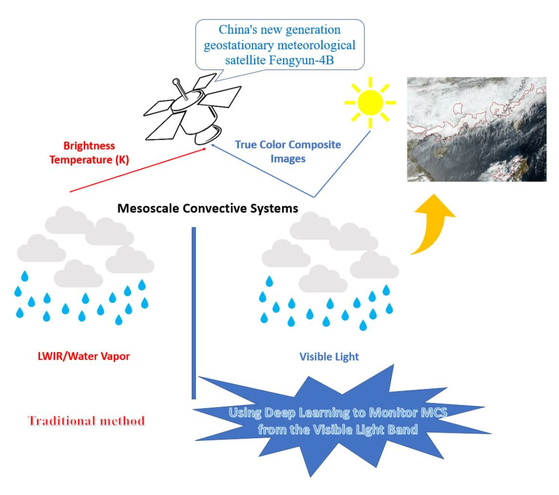
1. Introduction
2. Data and Study Area
2.1. Fengyun-4B Geostationary Meteorological Satellite AGRI and GPM Precipitation Data
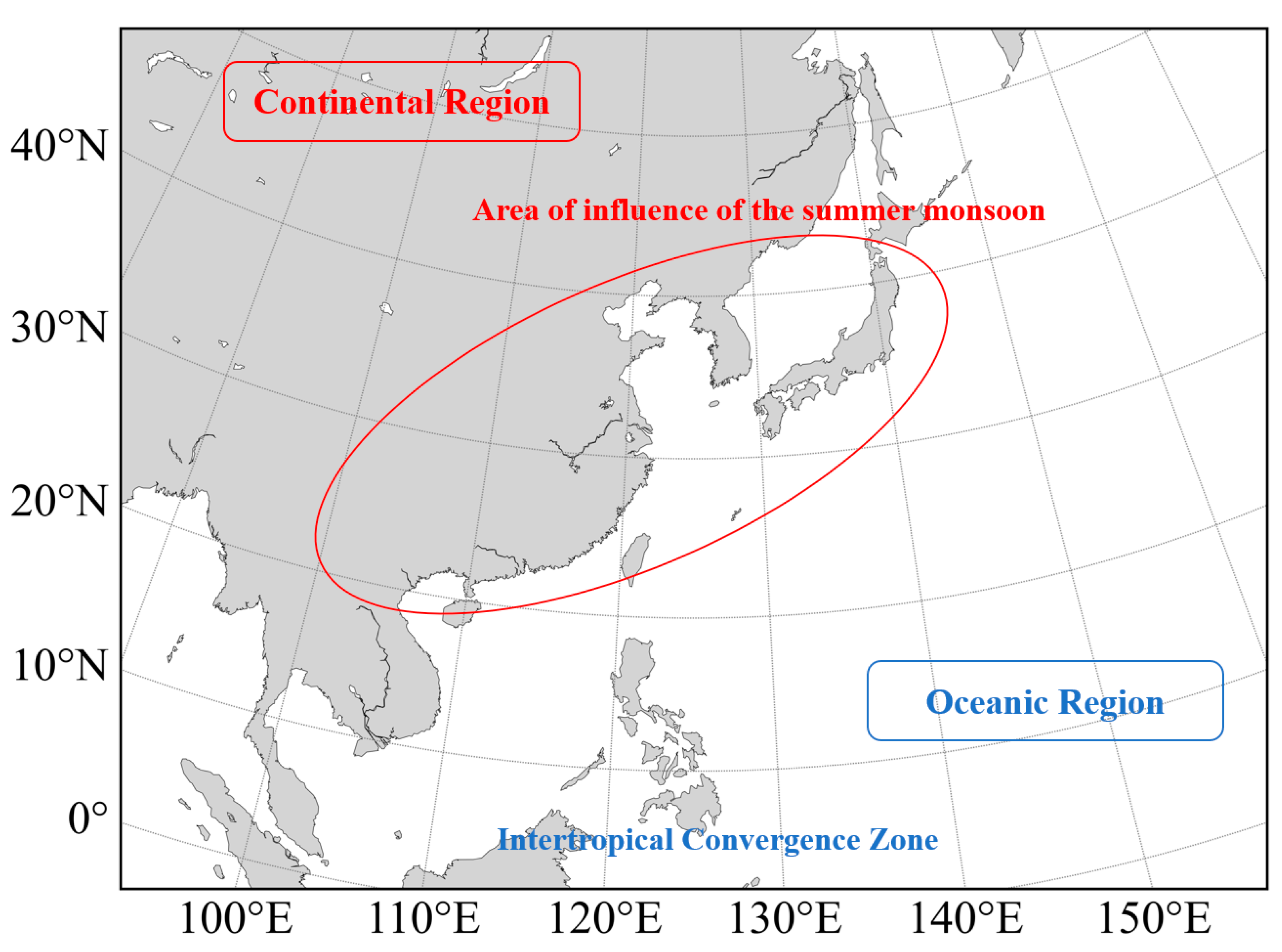
2.2. Study Area
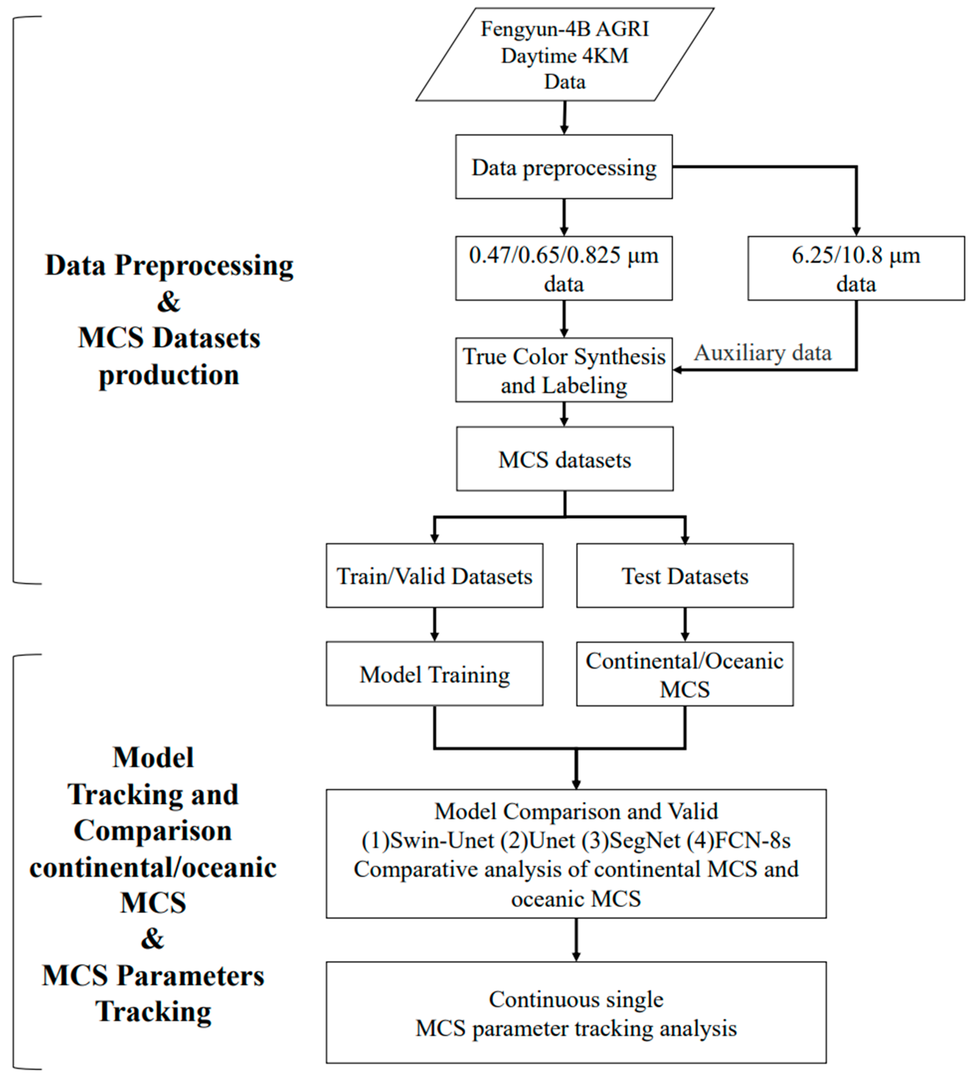
3. Method and Evaluation Metrics
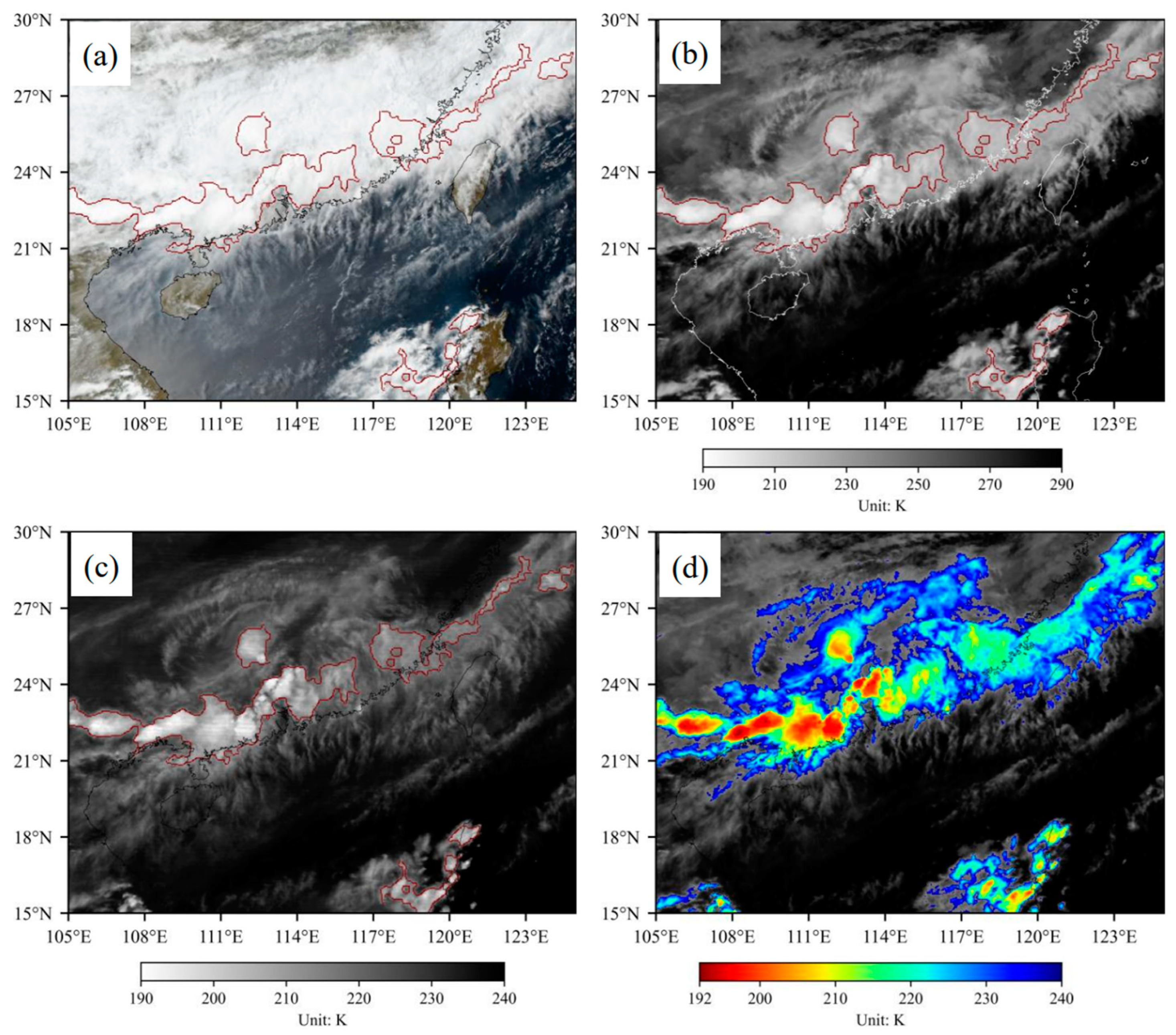
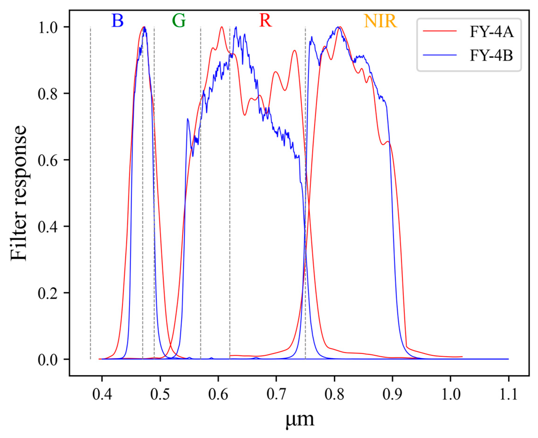
3.1. The Characteristics of MCS (Mesoscale Convective Systems) in Different Spectral Bands
3.2. Mesoscale Convective Systems (MCS) Label Dataset
3.3. Swin-Unet Model and Experimental Environment
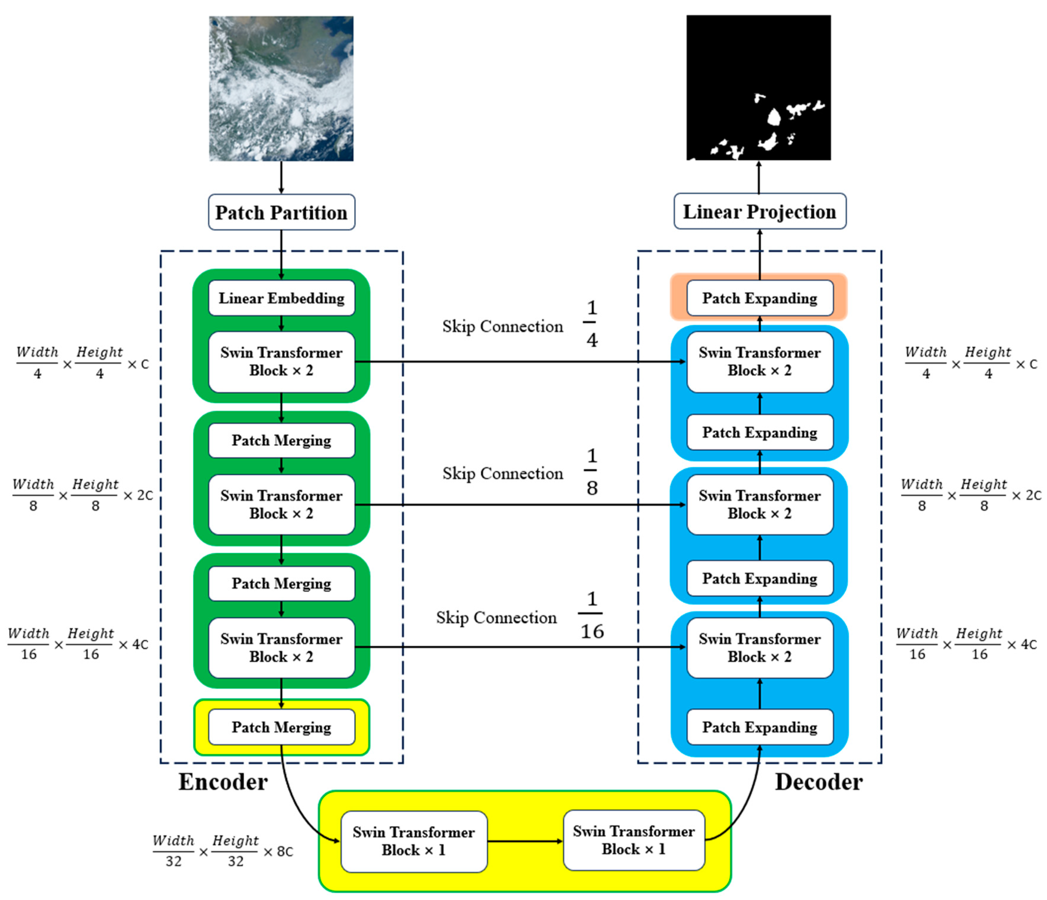
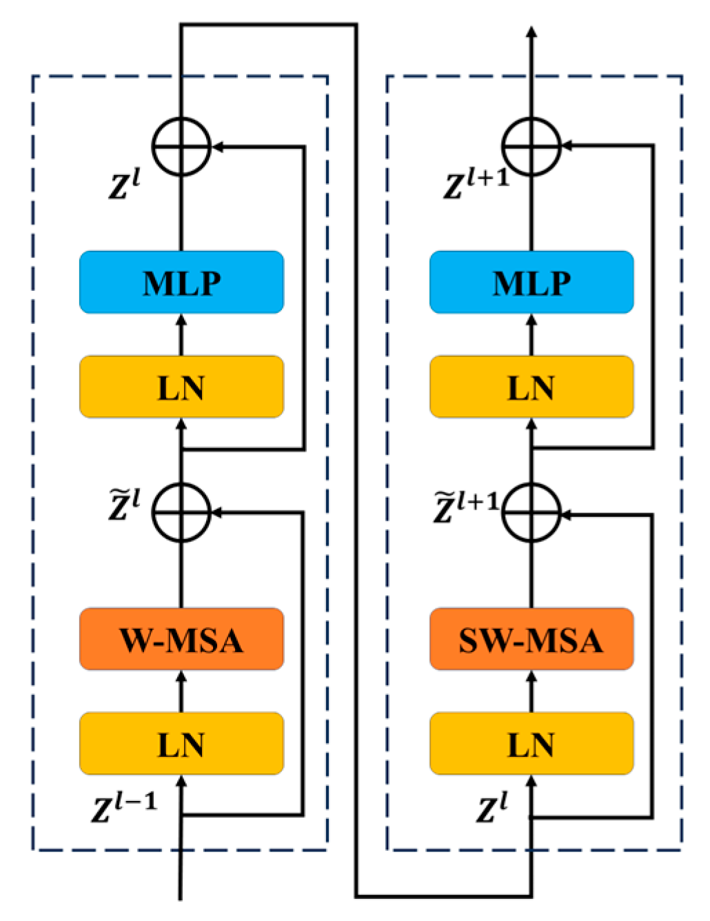
3.3.1. Swin-Unet
3.3.2. Experimental Environment
3.4. Evaluation Metrics
3.4.1. Recall
3.4.2. F1
3.4.3. IoU
3.4.4. FAR
4. Results
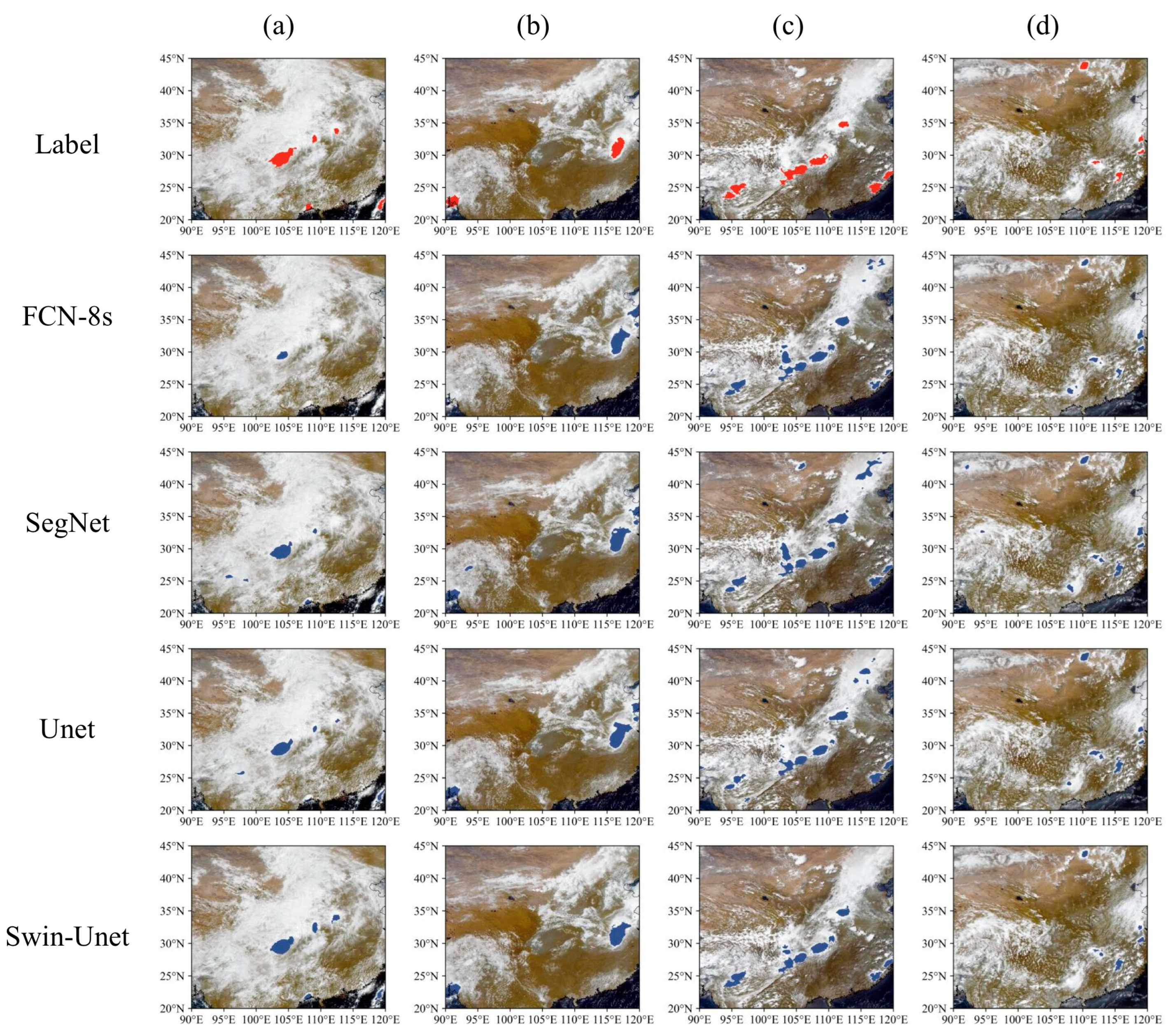
4.1. Swin-Unet Model Prediction Results for Continental MCS
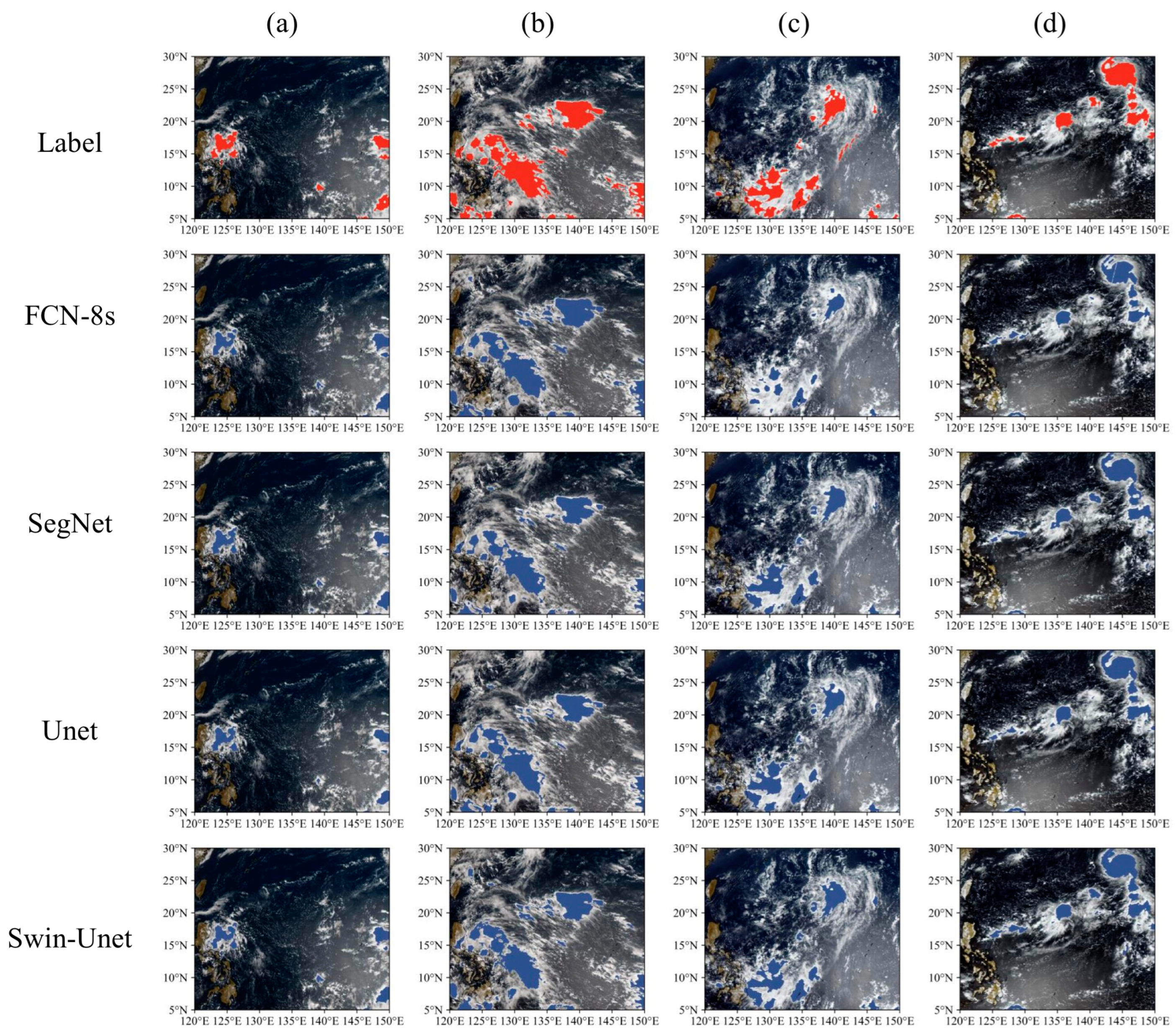
4.2. Swin-Unet Model Prediction Results for Oceanic MCS
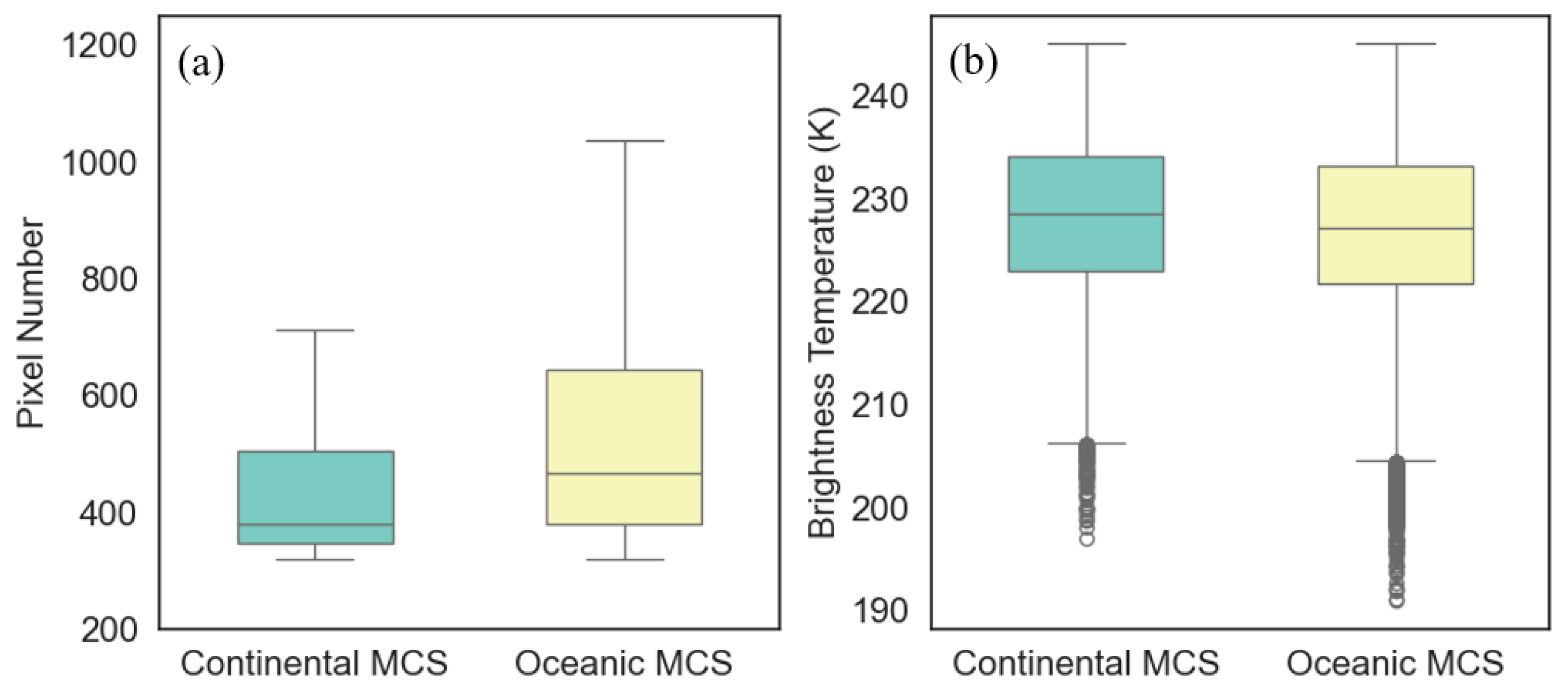
4.3. Comparative Analysis of Continental MCS and Oceanic MCS for the Test Dataset
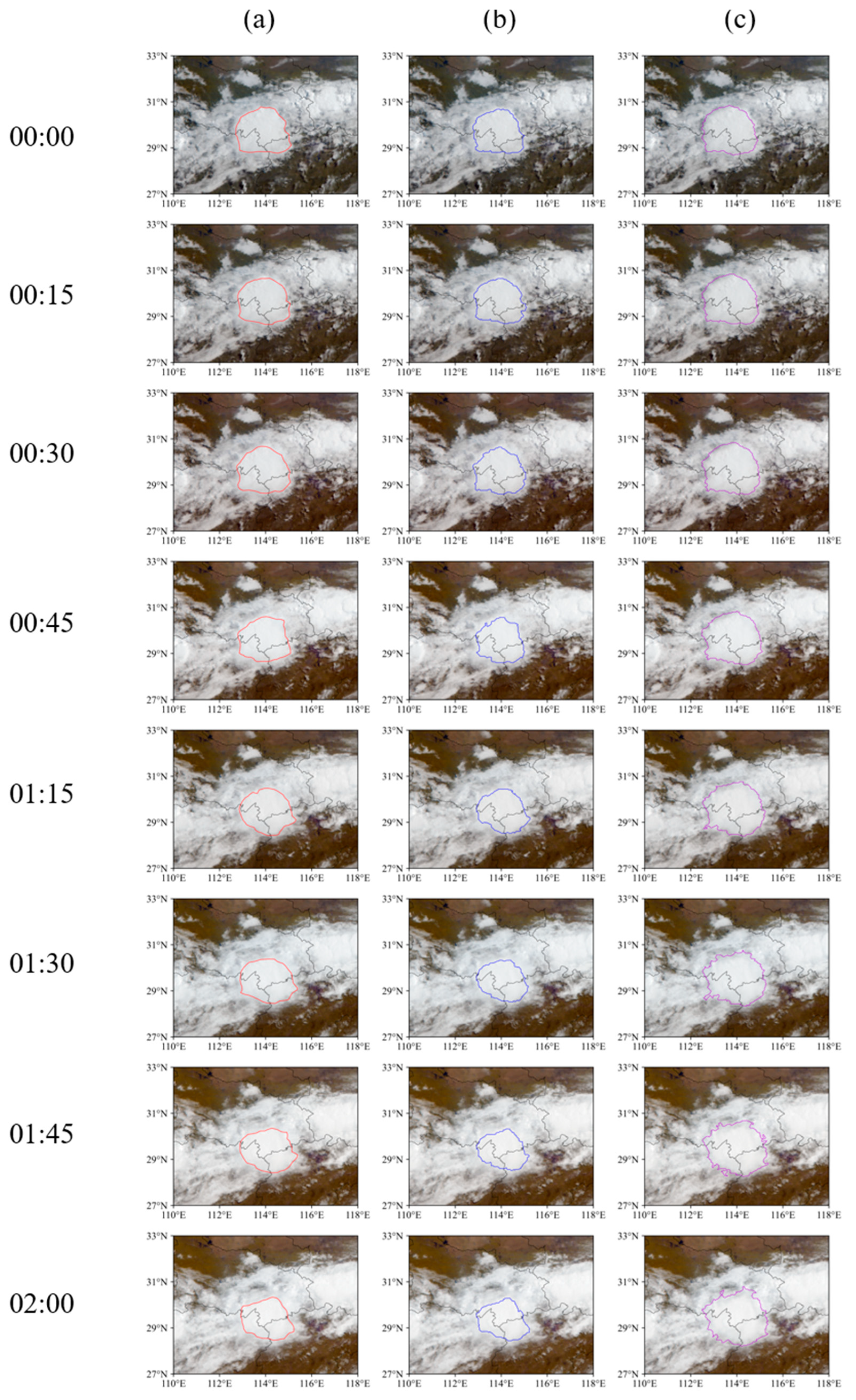
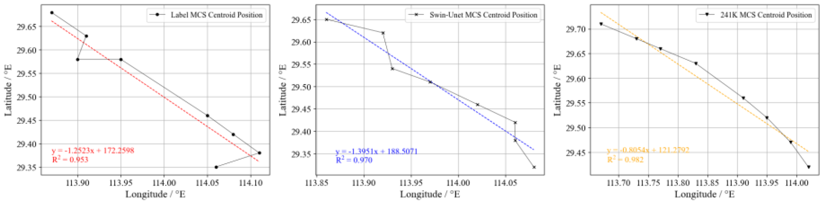
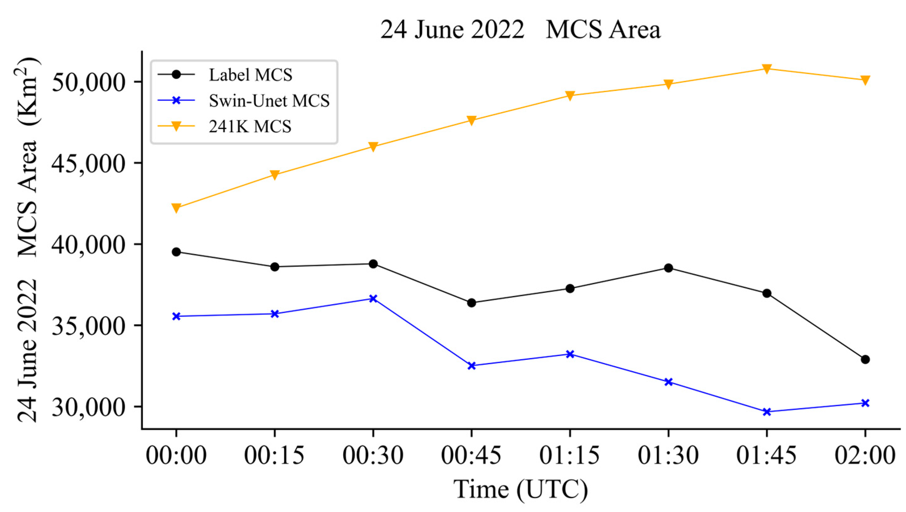
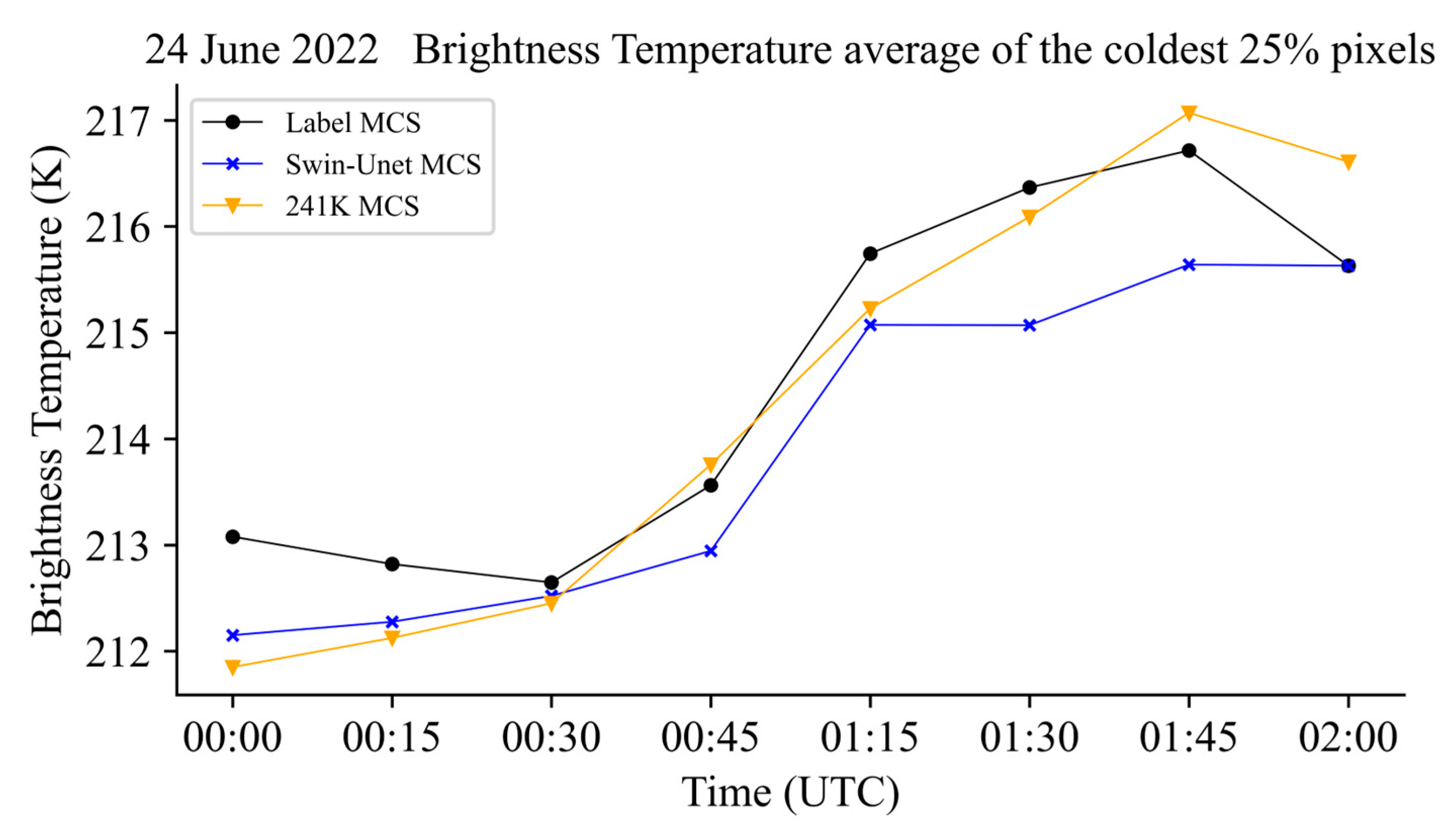
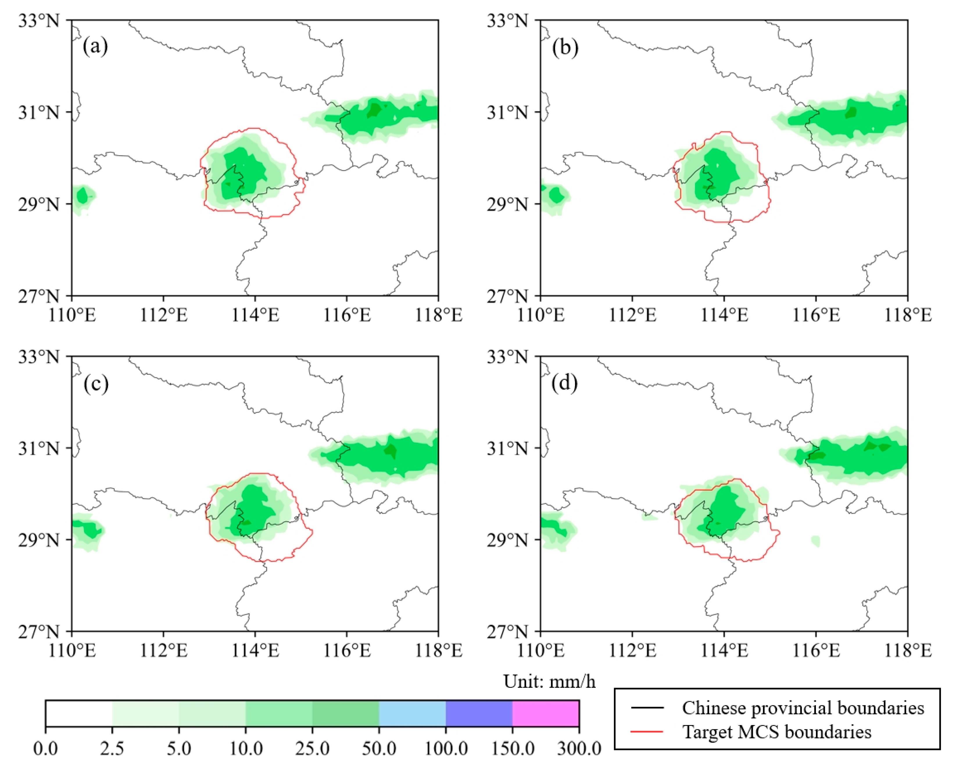
5. Case Study
6. Discussion
7. Conclusions
Author Contributions
Funding
Data Availability Statement
Acknowledgments
Conflicts of Interest
References
- Maddox, R.A. Mesoscale convective complexes. Bull. Am. Meteorol. Soc. 1980, 61, 1374–1387. [Google Scholar] [CrossRef]
- Anderson, C.J.; Arritt, R.W. Mesoscale convective complexes and persistent elongated convective systems over the United States during 1992 and 1993. Mon. Weather. Rev. 1998, 126, 578–599. [Google Scholar] [CrossRef]
- Jirak, I.L.; Cotton, W.R.; McAnelly, R.L. Satellite and radar survey of mesoscale convective system development. Mon. Weather. Rev. 2003, 131, 2428–2449. [Google Scholar] [CrossRef]
- Schumacher, R.S.; Rasmussen, K.L. The formation, character and changing nature of mesoscale convective systems. Nat. Rev. Earth Environ. 2020, 1, 300–314. [Google Scholar] [CrossRef]
- Augustine, J.A.; Howard, K.W. Mesoscale convective complexes over the United States during 1986 and 1987. Mon. Weather. Rev. 1991, 119, 1575–1589. [Google Scholar] [CrossRef]
- Feng, Z.; Leung, L.R.; Liu, N.; Wang, J.; Houze Jr, R.A.; Li, J.; Hardin, J.C.; Chen, D.; Guo, J. A global high-resolution mesoscale convective system database using satellite-derived cloud tops, surface precipitation, and tracking. J. Geophys. Res. Atmos. 2021, 126, e2020JD034202. [Google Scholar] [CrossRef]
- Wang, D.; Giangrande, S.E.; Feng, Z.; Hardin, J.C.; Prein, A.F. Updraft and downdraft core size and intensity as revealed by radar wind profilers: MCS observations and idealized model comparisons. J. Geophys. Res. Atmos. 2020, 125, e2019JD031774. [Google Scholar] [CrossRef]
- Yanase, W.; Shimada, U.; Kitabatake, N.; Tochimoto, E. Tropical Transition of Tropical Storm Kirogi (2012) over the Western North Pacific: Synoptic Analysis and Mesoscale Simulation. Mon. Weather. Rev. 2023, 151, 2549–2572. [Google Scholar] [CrossRef]
- Ryzhkov, A.; Zmic, D. Observations of a MCS with a dual-polarization radar. In Proceedings of the Proceedings of IGARSS’94-1994 IEEE International Geoscience and Remote Sensing Symposium, Pasadena, CA, USA, 8–12 August 1994; pp. 375–377. [Google Scholar]
- Hagen, M.; Schiesser, H.-H.; Dorninger, M. Monitoring of mesoscale precipitation systems in the Alps and the northern Alpine foreland by radar and rain gauges. Meteorol. Atmos. Phys. 2000, 72, 87–100. [Google Scholar] [CrossRef]
- Roberts, R.D.; Rutledge, S. Nowcasting storm initiation and growth using GOES-8 and WSR-88D data. Weather. Forecast. 2003, 18, 562–584. [Google Scholar] [CrossRef]
- Roberts, R.D.; Anderson, A.R.; Nelson, E.; Brown, B.G.; Wilson, J.W.; Pocernich, M.; Saxen, T. Impacts of forecaster involvement on convective storm initiation and evolution nowcasting. Weather. Forecast. 2012, 27, 1061–1089. [Google Scholar] [CrossRef]
- Walker, J.R.; MacKenzie, W.M.; Mecikalski, J.R.; Jewett, C.P. An Enhanced Geostationary Satellite–Based Convective Initiation Algorithm for 0–2-h Nowcasting with Object Tracking. J. Appl. Meteorol. Climatol. 2012, 51, 1931–1949. [Google Scholar] [CrossRef]
- Zhuge, X.; Zou, X. Summertime convective initiation nowcasting over southeastern China based on Advanced Himawari Imager observations. J. Meteorol. Soc. Japan Ser. II 2018, 96, 337–353. [Google Scholar] [CrossRef]
- Sun, H.; Wang, H.; Yang, J.; Zeng, Y.; Zhang, Q.; Liu, Y.; Gu, J.; Huang, S. Improving Forecast of Severe Oceanic Mesoscale Convective Systems Using FY-4A Lightning Data Assimilation with WRF-FDDA. Remote Sens. 2022, 14, 1965. [Google Scholar] [CrossRef]
- Zhang, X.; Shen, W.; Zhuge, X.; Yang, S.; Chen, Y.; Wang, Y.; Chen, T.; Zhang, S. Statistical characteristics of mesoscale convective systems initiated over the Tibetan Plateau in summer by Fengyun satellite and precipitation estimates. Remote Sens. 2021, 13, 1652. [Google Scholar] [CrossRef]
- Hui, W.; Guo, Q. Preliminary characteristics of measurements from Fengyun-4A Lightning Mapping Imager. Int. J. Remote Sens. 2021, 42, 4922–4941. [Google Scholar] [CrossRef]
- Hidayat, A.; Efendi, U.; Rahmadini, H.; Nugraheni, I. The Characteristics of squall line over Indonesia and its vicinity based on Himawari-8 satellite imagery and radar data interpretation. Proc. IOP Conf. Ser. Earth Environ. Sci. 2019, 303, 012059. [Google Scholar] [CrossRef]
- Chen, D.; Guo, J.; Yao, D.; Lin, Y.; Zhao, C.; Min, M.; Xu, H.; Liu, L.; Huang, X.; Chen, T. Mesoscale convective systems in the Asian monsoon region from Advanced Himawari Imager: Algorithms and preliminary results. J. Geophys. Res. Atmos. 2019, 124, 2210–2234. [Google Scholar] [CrossRef]
- Vila, D.A.; Machado, L.A.T.; Laurent, H.; Velasco, I. Forecast and Tracking the Evolution of Cloud Clusters (ForTraCC) using satellite infrared imagery: Methodology and validation. Weather. Forecast. 2008, 23, 233–245. [Google Scholar] [CrossRef]
- Song, F.; Feng, Z.; Leung, L.R.; Pokharel, B.; Wang, S.Y.S.; Chen, X.; Sakaguchi, K.; Wang, C.c. Crucial roles of eastward propagating environments in the summer MCS initiation over the US Great Plains. J. Geophys. Res. Atmos. 2021, 126, e2021JD034991. [Google Scholar] [CrossRef]
- Chen, S.-J.; Lee, D.-K.; Tao, Z.-Y.; Kuo, Y.-H. Mesoscale convective system over the yellow sea–a numerical case study. Meteorol. Atmos. Phys. 1999, 70, 185–199. [Google Scholar] [CrossRef]
- Zengping, F.; Yongguang, Z.; Yan, Z.; Hongqing, W. MCS census and modification of MCS definition based on geostationary satellite infrared imagery. J. Appl. Meteorol. Sci. 2008, 19, 82–90. [Google Scholar]
- Murakami, M. Analysis of the deep convective activity over the western Pacific and southeast Asia Part I: Diurnal variation. J. Meteorol. Soc. Japan. Ser. II 1983, 61, 60–76. [Google Scholar] [CrossRef]
- Fu, R.; Del Genio, A.D.; Rossow, W.B. Behavior of deep convective clouds in the tropical Pacific deduced from ISCCP radiances. J. Clim. 1990, 3, 1129–1152. [Google Scholar] [CrossRef]
- Hall, T.J.; Haar, T.H.V. The diurnal cycle of west Pacific deep convection and its relation to the spatial and temporal variation of tropical MCSs. J. Atmos. Sci. 1999, 56, 3401–3415. [Google Scholar] [CrossRef]
- Schmetz, J.; Tjemkes, S.; Gube, M.; Van de Berg, L. Monitoring deep convection and convective overshooting with METEOSAT. Adv. Space Res. 1997, 19, 433–441. [Google Scholar] [CrossRef]
- Setvák, M.; Rabin, R.M.; Wang, P.K. Contribution of the MODIS instrument to observations of deep convective storms and stratospheric moisture detection in GOES and MSG imagery. Atmos. Res. 2007, 83, 505–518. [Google Scholar] [CrossRef]
- Zheng, Y.; Yang, X.; Li, Z. Detection of severe convective cloud over sea surface from geostationary meteorological satellite images based on deep learning. J. Remote Sens. (Chin.) 2020, 24, 97–106. [Google Scholar] [CrossRef]
- Yang, Y.; Wu, X.; Wang, X. The sea-land characteristics of deep convections and convective overshootings over China sea and surrounding areas based on the CloudSat and FY-2E datasets. Acta Meteorol. Sin. 2019, 77, 256–267. [Google Scholar]
- Vaswani, A.; Shazeer, N.; Parmar, N.; Uszkoreit, J.; Jones, L.; Gomez, A.N.; Kaiser, Ł.; Polosukhin, I. Attention is all you need. arXiv 2017, arXiv:1706.03762. [Google Scholar]
- Dosovitskiy, A.; Beyer, L.; Kolesnikov, A.; Weissenborn, D.; Zhai, X.; Unterthiner, T.; Dehghani, M.; Minderer, M.; Heigold, G.; Gelly, S. An image is worth 16x16 words: Transformers for image recognition at scale. arXiv 2020, arXiv:2010.11929. [Google Scholar]
- Liu, Z.; Lin, Y.; Cao, Y.; Hu, H.; Wei, Y.; Zhang, Z.; Lin, S.; Guo, B. Swin transformer: Hierarchical vision transformer using shifted windows. In Proceedings of the IEEE/CVF International Conference on Computer Vision, Montreal, QC, Canada, 10–17 October 2021; pp. 10012–10022. [Google Scholar]
- Chen, J.; Lu, Y.; Yu, Q.; Luo, X.; Adeli, E.; Wang, Y.; Lu, L.; Yuille, A.L.; Zhou, Y. Transunet: Transformers make strong encoders for medical image segmentation. arXiv 2021, arXiv:2102.04306. [Google Scholar]
- Cao, H.; Wang, Y.; Chen, J.; Jiang, D.; Zhang, X.; Tian, Q.; Wang, M. Swin-unet: Unet-like pure transformer for medical image segmentation. In Proceedings of the European Conference on Computer Vision, Tel Aviv, Israel, 23–27 October 2022; pp. 205–218. [Google Scholar]
- Min, M.; Wu, C.; Li, C.; Liu, H.; Xu, N.; Wu, X.; Chen, L.; Wang, F.; Sun, F.; Qin, D. Developing the science product algorithm testbed for Chinese next-generation geostationary meteorological satellites: Fengyun-4 series. J. Meteorol. Res. 2017, 31, 708–719. [Google Scholar] [CrossRef]
- Sun, F.; Li, B.; Min, M.; Qin, D. Deep Learning-Based Radar Composite Reflectivity Factor Estimations from Fengyun-4A Geostationary Satellite Observations. Remote Sens. 2021, 13, 2229. [Google Scholar] [CrossRef]
- Zhang, X.; Xu, D.; Liu, R.; Shen, F. Impacts of FY-4A AGRI Radiance Data Assimilation on the Forecast of the Super Typhoon “In-Fa” (2021). Remote Sens. 2022, 14, 4718. [Google Scholar]
- Kong, X.; Jiang, Z.; Ma, M.; Chen, N.; Chen, J.; Shen, X.; Bai, C. The temporal and spatial distribution of sea fog in offshore of China based on FY-4A satellite data. Proc. J. Phys. Conf. Ser. 2023, 2486, 012015. [Google Scholar] [CrossRef]
- Wang, W.; Qu, P.; Liu, Z. Mesoscale Characteristics Analysis of a Fog Case with Complete Weather Information Derived from FengYun-4A Data. Meteorol. Environ. Res. 2022, 13, 10–27. [Google Scholar]
- Yi, L.; Li, M.; Liu, S.; Shi, X.; Li, K.-F.; Bendix, J. Detection of dawn sea fog/low stratus using geostationary satellite imagery. Remote Sens. Environ. 2023, 294, 113622. [Google Scholar] [CrossRef]
- Sun, J.; Zhao, S.; Xu, G.; Meng, Q. Study on a mesoscale convective vortex causing heavy rainfall during the Mei-yu season in 2003. Adv. Atmos. Sci. 2010, 27, 1193–1209. [Google Scholar] [CrossRef]
- Zhang, T.; Lin, W.; Lin, Y.; Zhang, M.; Yu, H.; Cao, K.; Xue, W. Prediction of tropical cyclone genesis from mesoscale convective systems using machine learning. Weather. Forecast. 2019, 34, 1035–1049. [Google Scholar] [CrossRef]
- Yihui, D.; Chan, J.C. The East Asian summer monsoon: An overview. Meteorol. Atmos. Phys. 2005, 89, 117–142. [Google Scholar] [CrossRef]
- Xu, X.; Xue, M.; Wang, Y.; Huang, H. Mechanisms of secondary convection within a Mei-Yu frontal mesoscale convective system in eastern China. J. Geophys. Res. Atmos. 2017, 122, 47–64. [Google Scholar] [CrossRef]
- May, P.T.; Mather, J.H.; Vaughan, G.; Jakob, C. Characterizing oceanic convective cloud systems: The tropical warm pool international cloud experiment. Bull. Am. Meteorol. Soc. 2008, 89, 153–155. [Google Scholar] [CrossRef]
- Wang, K.; Chen, G.; Bi, X.; Shi, D.; Chen, K. Comparison of convective and stratiform precipitation properties in developing and nondeveloping tropical disturbances observed by the Global Precipitation Measurement over the western North Pacific. J. Meteorol. Soc. Japan. Ser. II 2020, 98, 1051–1067. [Google Scholar] [CrossRef]
- Jun, L.; Bin, W.; Dong-Hai, W. The characteristics of mesoscale convective systems (MCSs) over East Asia in warm seasons. Atmos. Ocean. Sci. Lett. 2012, 5, 102–107. [Google Scholar] [CrossRef]
- Gumley, L.; Descloitres, J.; Schmaltz, J. Creating Reprojected True Color MODIS Images: A Tutorial; University of Wisconsin–Madison: Madison, WI, USA, 2003; p. 19. [Google Scholar]
- Zhuge, X.-Y.; Zou, X.; Wang, Y. A fast cloud detection algorithm applicable to monitoring and nowcasting of daytime cloud systems. IEEE Trans. Geosci. Remote Sens. 2017, 55, 6111–6119. [Google Scholar] [CrossRef]
- Yan, J.; Qu, J.; Zhang, F.; Guo, X.; Wang, Y. Study on multi-dimensional dynamic hybrid imaging technology based on FY-4A/AGRI. J. Meteorol. Environ. 2022, 38, 98–105. [Google Scholar] [CrossRef]
- Huang, Y.; Zhang, M. Contrasting Mesoscale Convective System Features of Two Successive Warm-Sector Rainfall Episodes in Southeastern China: A Satellite Perspective. Remote Sens. 2022, 14, 5434. [Google Scholar] [CrossRef]


| Spectrum | Fengyun-4A | Fengyun-4B | Main Application | ||
|---|---|---|---|---|---|
| Channel | Central Wavelength (μm) | Channel | Central Wavelength (μm) | ||
| VIS/NIR | 1 | 0.47 μm | 1 | 0.47 μm | Aerosols, true color synthesis |
| 2 | 0.65 μm | 2 | 0.65 μm | True color synthesis | |
| 3 | 0.825 μm | 3 | 0.825 μm | True color synthesis | |
| SWIR | 4 | 1.375 μm | 4 | 1.379 μm | Cirrus |
| 5 | 1.61 μm | 5 | 1.61 μm | Distinguish low clouds and snow Cloud phase separation | |
| 6 | 2.25 μm | 6 | 2.25 μm | Cirrus, aerosols | |
| MIR | 7 | 3.75 μm (High) | 7 | 3.75 μm | High-albedo targets, fire points |
| 8 | 3.75 μm (Low) | 8 | 3.75 μm | Low-albedo targets, surface | |
| Water Vapor | 9 | 6.25 μm | 9 | 6.25 μm | High-level water vapor |
| 10 | 7.1 μm | 10 | 6.95 μm | Middle-level water vapor | |
| —— | 11 | 7.42 μm | Low-level water vapor | ||
| LWIR | 11 | 8.5 μm | 12 | 8.55 μm | Clouds |
| 12 | 10.7 μm | 13 | 10.8 μm | Clouds, LST | |
| 13 | 12.0 μm | 14 | 12 μm | Clouds, water vapor content, LST | |
| 14 | 13.5 μm | 15 | 13.3 μm | Clouds, water vapor | |
| Train/Valid Dataset | Train Clip Number | Test Dataset |
|---|---|---|
| 1–22 June 2022 | 18,076 (512 × 512 pixels) (Continental/Oceanic MCS) | 23–30 June 2022 |
| 1–23 July 2022 | 24–31 July 2022 | |
| 1–22 August 2022 | 23–31 August 2022 |
| Prediction MCS | Prediction Non-MCS | |
|---|---|---|
| Label MCS | TP (True positive) | FN (False negative) |
| Label non-MCS | FP (False positive) | TN (True negative) |
| Recall | F1 | IoU | FAR | |
|---|---|---|---|---|
| Swin-Unet | 83.37% | 72.9% | 57.46% | 33.96% |
| Unet | 83.19% | 68.43% | 52.09% | 37.11% |
| SegNet | 81.94% | 62.39% | 45.48% | 45.24% |
| FCN-8s | 59.93% | 51.68% | 36.37% | 36.81% |
| Recall | F1 | IoU | FAR | |
|---|---|---|---|---|
| Swin-Unet | 86.1% | 83.47% | 71.65% | 17.14% |
| Unet | 81.74% | 82.14% | 69.69% | 17.31% |
| SegNet | 80.46% | 82.76% | 70.63% | 14.73% |
| FCN-8s | 73.29% | 77.48% | 64.18% | 12.87% |
Disclaimer/Publisher’s Note: The statements, opinions and data contained in all publications are solely those of the individual author(s) and contributor(s) and not of MDPI and/or the editor(s). MDPI and/or the editor(s) disclaim responsibility for any injury to people or property resulting from any ideas, methods, instructions or products referred to in the content. |
© 2023 by the authors. Licensee MDPI, Basel, Switzerland. This article is an open access article distributed under the terms and conditions of the Creative Commons Attribution (CC BY) license (https://creativecommons.org/licenses/by/4.0/).
Share and Cite
Xiang, R.; Xie, T.; Bai, S.; Zhang, X.; Li, J.; Wang, M.; Wang, C. Monitoring Mesoscale Convective System Using Swin-Unet Network Based on Daytime True Color Composite Images of Fengyun-4B. Remote Sens. 2023, 15, 5572. https://doi.org/10.3390/rs15235572
Xiang R, Xie T, Bai S, Zhang X, Li J, Wang M, Wang C. Monitoring Mesoscale Convective System Using Swin-Unet Network Based on Daytime True Color Composite Images of Fengyun-4B. Remote Sensing. 2023; 15(23):5572. https://doi.org/10.3390/rs15235572
Chicago/Turabian StyleXiang, Ruxuanyi, Tao Xie, Shuying Bai, Xuehong Zhang, Jian Li, Minghua Wang, and Chao Wang. 2023. "Monitoring Mesoscale Convective System Using Swin-Unet Network Based on Daytime True Color Composite Images of Fengyun-4B" Remote Sensing 15, no. 23: 5572. https://doi.org/10.3390/rs15235572