Article

Detection of Atmospheric Hydrofluorocarbon-22 with Ground-Based Remote High-Resolution Fourier Transform Spectroscopy over Hefei and an Estimation of Emissions in the Yangtze River Delta

1
Key Laboratory of Environmental Optics and Technology, Anhui Institute of Optics and Fine Mechanics, Hefei Institutes of Physical Science, Chinese Academy of Sciences, Hefei 230031, China
2
University of Science and Technology of China, Hefei 230026, China
3
State Environmental Protection Key Laboratory of Sources and Control of Air Pollution Complex, Beijing 100084, China
4
Department of Automation, Hefei University, Hefei 230601, China
5
Department of Precision Machinery and Precision Instrumentation, University of Science and Technology of China, Hefei 230026, China
6
Anhui Province Key Laboratory of Polar Environment and Global Change, University of Science and Technology of China, Hefei 230026, China
7
Center for Excellence in Regional Atmospheric Environment, Institute of Urban Environment, Chinese Academy of Sciences, Xiamen 361021, China
8
Key Laboratory of Precision Scientific Instrumentation of Anhui Higher Education Institutes, University of Science and Technology of China, Hefei 230026, China
*
Author to whom correspondence should be addressed.
Remote Sens. 2023, 15(23), 5590; https://doi.org/10.3390/rs15235590
Submission received: 7 November 2023 / Revised: 28 November 2023 / Accepted: 29 November 2023 / Published: 30 November 2023
(This article belongs to the Special Issue Advances in Remote Sensing and Atmospheric Optics)

Abstract

:
Under the control of the Montreal Protocol and its amendments, hydrofluorocarbons (HCFCs) are used as temporary substitutes for ozone-depleting substances, such as chlorofluorocarbons, and are regulated for consumption and production. China plans to phase out HCFCs by 2030, and HCFC-22 (CHClF2) is currently the most abundant HCFC in the atmosphere. This study measures the vertical profiles and total columns of atmospheric HCFC-22 from January 2017 to December 2022, based on the mid-infrared solar spectra recorded by the ground-based high-resolution Fourier transform infrared (FTIR) spectrometer at the Hefei remote sensing station. The HCFC-22 total columns over Hefei increased from 2017–2018 and gradually decreased in 2018–2022, with an annual variation rate of 5.98% and −1.02% ± 0.02%, respectively. Compared with the ACE-FTS satellite independent dataset, the FTIR data indicate good consistency with the ACE-FTS data at a 5–25 km altitude, with an average relative difference of −4.38 ± 0.83% between the vertical profiles. HCFC-22 emissions in the Yangtze River Delta from 2017 to 2022 are estimated, derived from measured total columns combined with the Lagrangian transport model and the Bayesian inversion technique. In the Yangtze River Delta, HCFC-22 emissions were high in 2017, with a value of 33.3 ± 16.8 kt, and decreased from 2018 to 2022, with a minimum of 27.3 ± 13.6 kt in 2022 during the observations.

1. Introduction

Chlorodifluoromethane (CHClF2, HCFC-22) is a hydrofluorocarbon gas, commonly used in industrial and domestic refrigeration systems. Ever since Molina and Rowland (1974) confirmed that chlorofluorocarbons (CFCs) can severely destroy the ozone layer, scientists have been searching for more alternatives of chlorofluorocarbons [1]. According to the regulations of the Montreal Protocol on Substances that Deplete the Ozone Layer, HCFCs, as temporary substitutes for CFCs, have been widely used in industrial production since the early 21st century. The atmospheric lifetime of HCFC-22 is approximately 9.8–18 years. Compared to common CFCs, HCFC-22 has a shorter lifetime, but due to the presence of chlorine atoms, hydrofluorocarbons still have the potential to destroy the stratospheric ozone [2]. Meanwhile, HCFCs also have high greenhouse warming potentials (GWPs, the ratio of the emission radiative forcing of a substance to the same mass emission of CO2 summed within a given time period, with the GWP of CO2 equal to 1), which reported to be 1780 for 100 years (WMO, 2018) [3].
As one of the world’s largest HCFC-consuming countries, China accumulated approximately 1576.8 (1348.2–1819.0) kt of HCFC-22 emissions from 1990 to 2019 [4]. China promised to phase out the production of HCFC-22 completely before 2030, in order to adhere to the Montreal Protocol. A study of the HCFC-22 concentration trends and distributions in the atmosphere will help to understand HCFCs’ emissions in China. At present, the concentration measurement and regional emission estimate of HCFC-22 have attracted more attention in China [5,6,7,8,9]. Fang et al. (2019) estimated the emission and variations of major HCFCs in China from 2011–2017 based on HCFC-22 concentration data from seven in-situ stations and the Bayesian inversion technique [5]. Yu et al. (2022) used flask sampling to measure the HCFC-22 ambient mixing ratio at the Lin’an background station and estimated the regional emissions of HCFC-22 during 2011–2018, using the interspecies correlation method [6].
Compared with in-situ measurements, the Fourier transform infrared spectroscopy (FTIR) technology is employed for the remote sensing of the HCFC’s column concentration. For satellite remote sensing, the limb-viewing infrared Fourier transform spectrometer MIPAS (Michelson Interferometer for Passive Atmospheric Sounding) observed the global HCFC-22 on the Environmental Satellite (ENVISAT) from 2002–2012 [10,11,12]. The Atmospheric Chemistry Experiment-Fourier Transform Spectrometer (ACE-FTS) has been monitoring the global HCFC-22 atmospheric concentration since 2003 [13,14,15,16,17]. Steffen et al. (2019) analyzed the HCFC-22 annual trend changes in the tropical region between 7.5–17.5 km in 2004–2018 for ACE-FTS satellite data [17].
Réunion Island, Jungfraujoch, and the St. Petersburg site are applying ground-based high-resolution FTIR technology to measure HCFC-22’s spatial distribution and long-term trends, and the total columns of HCFC-22 show good consistency in comparison with satellite data [18,19,20]. Zhou et al. (2016) operated ground-based FTIR instruments to detect HCFC-22 above two NDACC stations at Réunion Island and compared the results with MIPAS/ENVISAT data [18]. Prignon et al. (2019) retrieved HCFC-22 above Jungfraujoch using the improved retrieval strategy and analyzed the results with model simulations, in-situ measurements, and satellite data [19]. Polyakov et al. (2021) observed HCFC-22 total columns at the St. Petersburg site and compared WACCM data and ACE-FTS data with high-resolution FTIR data [20].
The Hefei FTIR station is one of the candidate NDACC (Network for the Detection of Atmospheric Composition Change) stations. Hefei, located in the Yangtze River Delta, is one of the most developed regions in China. The Yangtze River Delta includes the Shanghai municipality and the provinces of Jiangsu, Zhejiang, and Anhui, accounting for 3.7% of China’s total area with a population of 227 million, and constituted about a quarter of the country’s GDP in 2019 [21]. The Yangtze River Delta has a manufacturing industry with a strong production capacity and a high industrialization level. According to statistics, 60% of HCFC-22-production enterprises in China are located in the region (National Development and Reform Commission, 2018) [22]. A high production of HCFC-22 that is caused by a large population and high industrialization may lead to high HCFC-22 emissions in the region. Therefore, an understanding of the HCFC-22 emissions in the Yangtze River Delta is of great significance for studying HCFC emissions in China.
The purpose of this study is to retrieve HCFC-22’s spatio-temporal distribution from solar spectra using ground-based Fourier transform infrared spectroscopy, to compare the total columns with the ACE-FTS satellite database, and then to obtain HCFC-22 emissions in the Yangtze River Delta based on measured data. Section 2 introduced the Hefei FTIR observation station, as well as the retrieval parameters and strategies of HCFC-22. Provided the single spectral retrieval of HCFC-22, understood the basic knowledge of ACE-FTS satellite, Lagrangian particle diffusion model FLEXPART and Bayesian algorithm. Section 3 studied the interannual variation and seasonal results of HCFC-22, compared the data with ACE-FTS satellite data, and estimated the HCFC-22 emissions in the Yangtze River Delta. Section 4 discussed the above results. Section 5 provided the conclusions from this study.

2. Materials and Methods

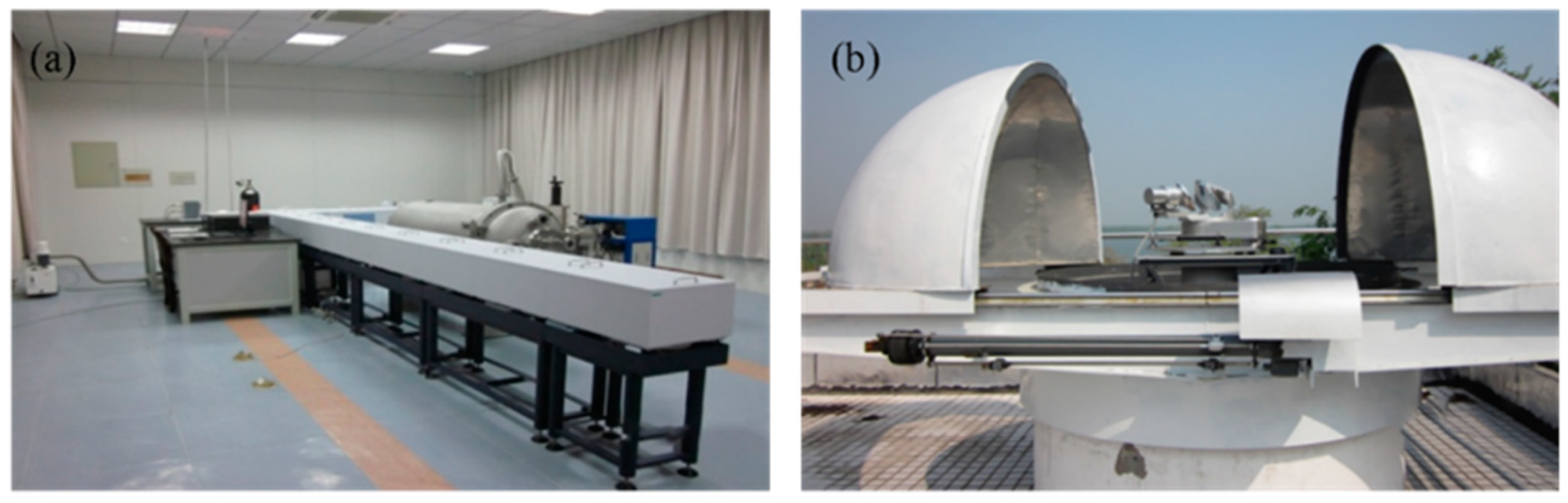
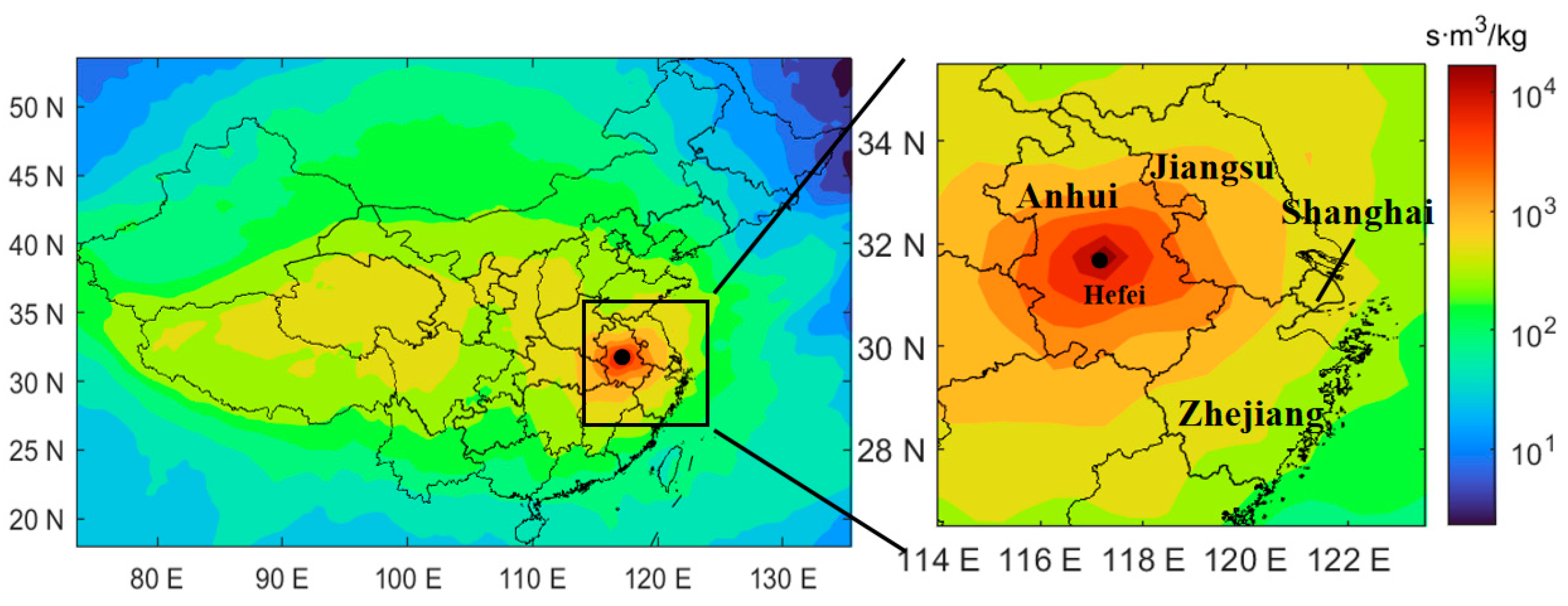
2.1. Site Description

The Hefei site is located in the north-west suburbs of Hefei, Anhui in eastern China (31.91°N and 117.17°E). Our site installed a high-resolution FTIR spectrometer (Bruker IFS 125HR), matched with a solar tracker (A547), to sample solar absorption infrared spectra since 2014, as shown in Figure 1 [23]. We installed the Zeno meteorological station (coastal environmental systems, Seattle, WA, USA) to record meteorological information [24].
The Hefei high-resolution FTIR observation station is an NDACC-IRWG candidate station and has been widely used for studying atmospheric trace gases and for verifying satellite data and model simulations [25,26,27,28]. The main spectrum in this study is the mid-infrared spectrum, which has a spectral resolution of 0.005 cm−1. The high-resolution FTIR spectrometer in this study was equipped with a mercury cadmium telluride (MCT) detector and a KBr beamsplitter. We replaced the CaF2 incoming light window of the FTIR spectrometer with the KCl window in December 2016, so we could measure the mid-infrared spectrum in the 700–4000 cm−1 range since then.

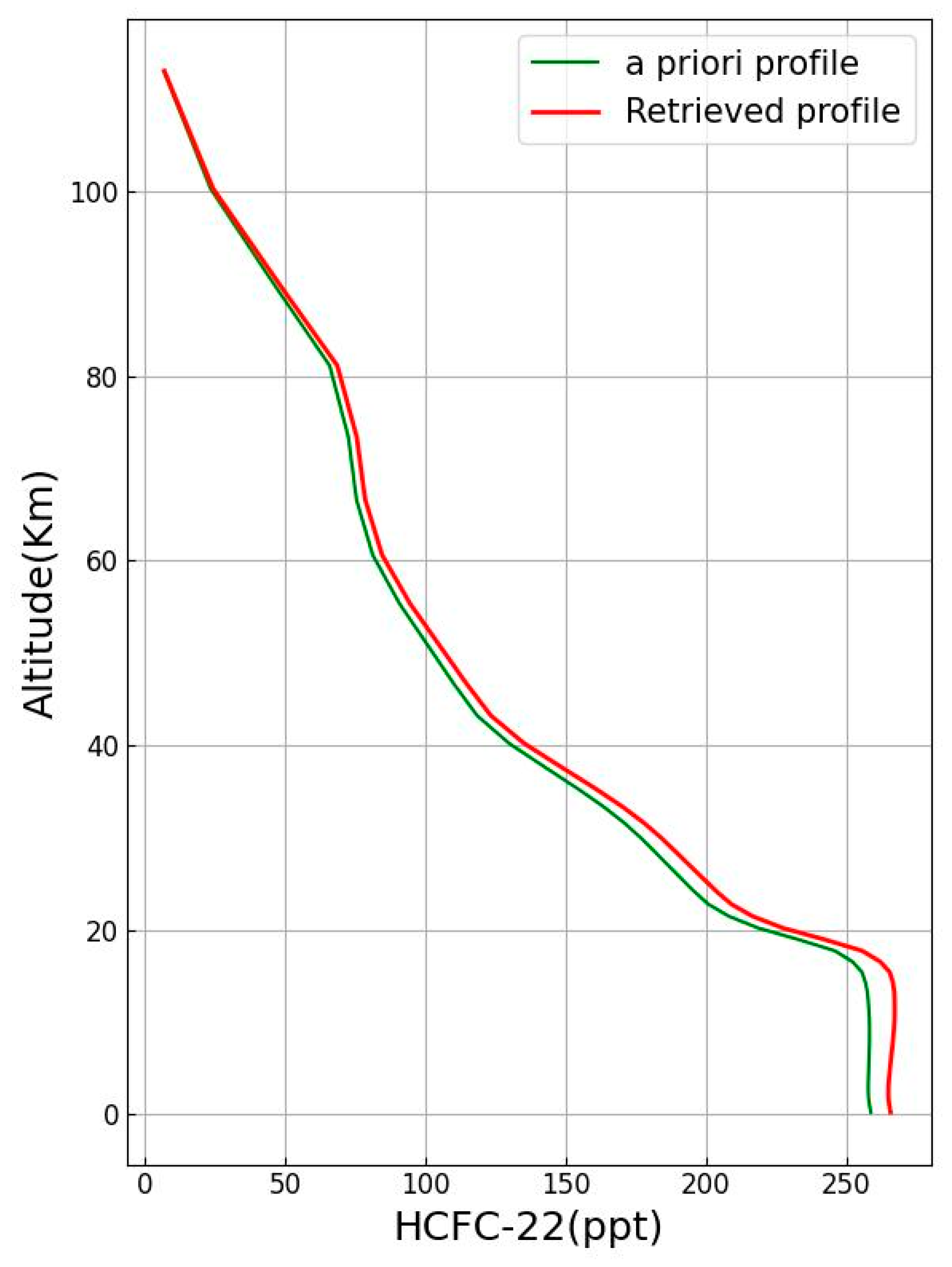
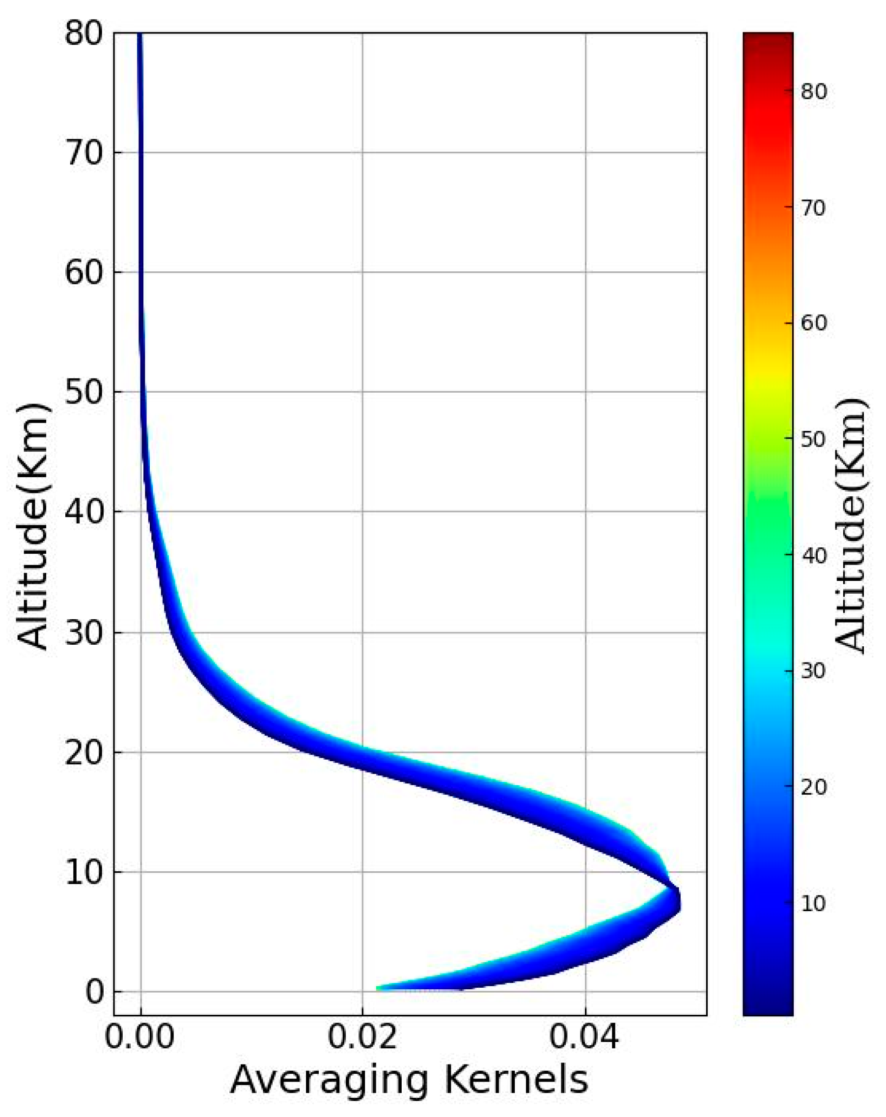
2.2. HCFC-22 Retrieval Strategy

The retrieval microwindow of HCFC-22 is 2ν6 Q-branch (828.75–829.4 cm−1), and HCFC-22 has relatively strong absorption features in this infrared spectral region. The pseudo-line list (PLL) from the NASA laboratory is used to calculate the spectroscopic line parameter of HCFC-22 [29]. The interfering gases include H2O, CO2, and O3, and the line parameters were calculated using HITRAN 2012. The reanalysis data of the National Centers for Environment Protection (NCEP) provides the main atmospheric parameters used in retrieval [30]. All prior gas profiles, except for H2O, are from WACCM version 6 data [31]. Table 1 lists the retrieval parameters.
The SFIT4 (version 0.9.4.4) algorithm is used to retrieve the total columns and vertical profile of HCFC-22 [32]. This algorithm is based on the optimal estimation method (OEM). The relationship between the measurement vector y and the state vector x is described as follows:
y = F x , b + ε
F x , b   is the forward model, which describes the entire physical process of the measurement; state vector x represents the vertical profile of the gas needed to be retrieved; b contains information that may affect the measurement vector; and ε represents the measurement noise and uncertainty. The F x , b in the FTIR measurement is nonlinear, so the algorithm uses Newton’s iteration method to ultimately find the state vector x ^ that is close to the real state vector x :
x ^ = x a + A ( x x a ) + ε
x a is an a priori profile from WACCM version 6. The averaging kernel matrix A denotes, as the sensitivity, the retrieved states and is described as follows:
A = S a 1 + K T S ε 1 K ) 1 K T S ε 1 K
After using the i + 1 iterations by the Newton’s iteration method, the optimal solution of the state vector is obtained:
x i + 1 = x i + K i T S ε 1 K i + S a 1 1 × K i T S ε 1 y F ( x i ) S a 1 ( x i x a )
K is the weight function matrix; S a is the priori covariance matrix, and its inverse matrix is the regularization matrix R ; and S ε represents the measurement covariance matrix. The regularization matrix required for the algorithm is calculated through the Tikhonov L 1 regularization method in our study, and L 1 is the first derivative operator. As described by Tikhonov and Sussmann, the regularization matrix R is defined as follows [33,34]:
R = α L 1 T L 1
when the height is a non-height constant search grid:
R = α L 1 T T L 1
where α is the regularization strength, and T is calculated by the thickness of the different layers ( z ):
T = 1 z 1 2 0 0 1 z 2 2 0 0 0 0 1 z n 1 2 R ( n 1 ) × ( n 1 )
In order to minimize measurement errors and smoothing errors, we chose the regularization strength α as 100 for HCFC-22’s retrieval.

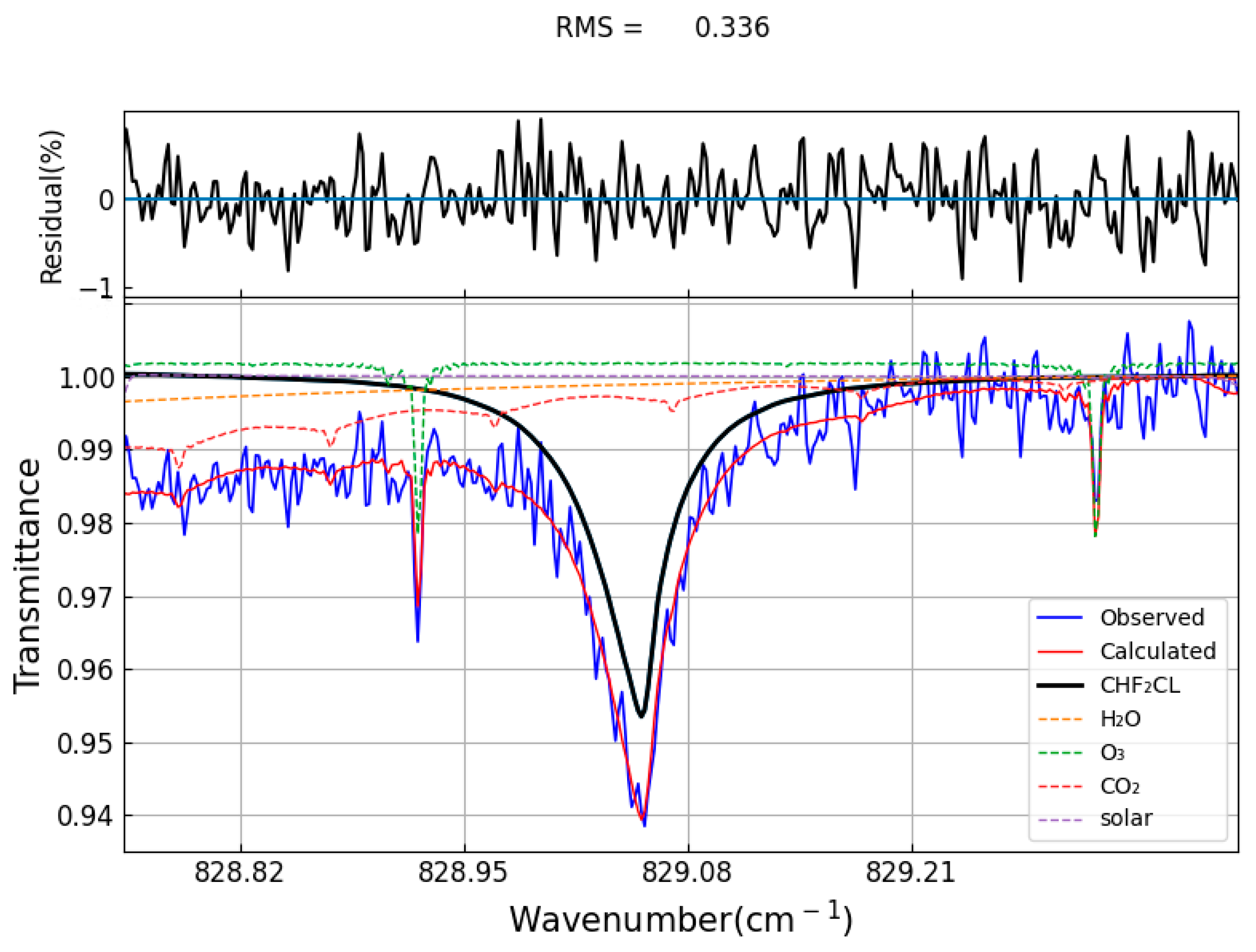
2.3. Typical Spectral Retrieval of HCFC-22

Figure 2 shows the typical spectral fitting obtained from the mid-infrared spectrum collected on 2 January 2022 at 02:45:14 UTC (solar zenith angle, SZA is 58.69°). The variation-of-fitting residual is within ±1%, and the RMS (root-mean-square) is 0.336%. As shown in Figure 3, HCFC-22 is mainly collected below 20 km and has a relatively low variation, and the concentration gradually decreases from the altitude of 20 km to the higher altitudes. The average kernel of HCFC-22 represents the impact of concentration changes at each layer height on the concentration retrieval at other layers, i.e., the sensitivity of retrieval at that height. It can be seen that the average kernel is high below the 20 km altitude, reaching the highest value at around an 8 km altitude in Figure 4.
In the error analysis of HCFC-22’s retrieval, the posteriori error estimation method from Rodgers (2003) [35] mainly includes the smoothing error ( S s ),
S s = ( A I ) S e ( A I ) T
the forward model parameter error ( S f ),
S f = G y K b S b K b T G y T
and the measurement error ( S m ),
S m = G y S ε G y T
where G y is the contribution matrix, K b is the weight function of the forward model on the model parameters, S e is the retrieval’s state vector covariance matrix, S b represents the forward model parameter matrix, and S ε is the measurement covariance matrix [35].
Table 2 shows the calculated error terms of HCFC-22’s retrieval, including systematic errors and random errors. For the uncertainty setting of the error term, the vertical profile’s systematic uncertainty of atmospheric temperature is calculated from NCEP. The random error of the entire atmospheric temperature is 5 K. The systematic error uncertainty parameter of SZA is selected as 0.1°, while the random uncertainty is 0.2°. The maximum absorption coefficient error of HCFC-22 in the PLL is 5%. Therefore, the priori error-of-line-intensity error, the Line T-broadening error, and the Line P-broadening error are also set to 5%. The uncertainty of the H2O spectroscopy, the instrument line shape (ILS), and the zero-level offset (zshift) are set to 10%, 2%, and 1%, respectively.
The systematic error for the HCFC-22 typical retrieval at Hefei is 3.8%, and the random error is 2.6%. H2O spectroscopy is the main systematic error, and then measurement error is the main source of random error. The total error of typical HCFC-22 retrieval is 4.6%, which means that our retrieval results are reasonable. The total systematic/random uncertainties for the HCFC-22 retrievals are 4.7/4.4% at the St. Denis site, 4.4/3.6% at the Maïdo site, and 5.75/3.70% at the St. Petersburg site [18,20]. The typical systematic and random errors for the Hefei HCFC-22 retrievals are similar to the other sites.

2.4. ACE (Atmospheric Chemistry Experience) Satellite Data

The primary objective of the ACE (Atmospheric Chemistry Experience) satellite is to understand the impact of ozone-depleting substances on the ozone and to study the chemical and dynamical processes of the ozone in the stratosphere and upper troposphere. The mission of ACE is to observe the atmospheric ozone-depletion components, such as CFCs and HCFCs. ACE-FTS covers the 750–4400 cm−1 range and operates the solar occultation to collect atmospheric transmission spectra at sunrise or sunset. The vertical resolution of the ACE-FTS data is approximately 4 km [36,37].
The ACE focus regions are mainly in the Arctic and high latitude regions, and the observation data in the tropical and subtropical regions are little [38]. To obtain more comparable satellite data, we chose the satellite data of ±5° latitudes and ±10° longitudes (27–37°N and 107–127°E) centered on the Hefei station, and the FTIR data with a satellite transit time of ±2 days to compare the HCFC-22 vertical profiles from 2017–2022. The ACE data (v4.1/v4.2) were used, and the outliers were filtered by eliminating the points deviating from 2.5 times the median absolute deviations [15]. Considering the difference in a prior profile and the vertical sensitivity between two measurements, it is necessary to interpolate the satellite profile into the FTIR vertical grid before comparing the two datasets and then to smooth the satellite data to obtain the smoothed satellite profile x sat [35]:
x sat = x a + A ( x sat x a )
x a represents a prior profile of FTIR, x sat is the raw satellite profile, and A is the FTIR-averaging kernels matrix.

2.5. Atmospheric Transport Simulation

The Lagrangian particle dispersion model FLEXPART, developed in the 1990s, has been widely applied in multi-scale atmospheric transport simulations and analyses for atmospheric gases and aerosols. FLEXPART simulates the transport and diffusion of tracer releases, and inverse modeling, derived from source receptor relationships, is commonly used in atmospheric research [39,40,41]. In FLEXPART’s backward mode, we calculated the sensitivity of receptor elements to the source and obtained the influence of mass emissions at the source location on the atmospheric mixing ratio at the receptor location. In our study, the model is driven by wind field data from the European Centre for Medium-Range Weather Forecasts (ECMWFs) for 3 h and a 0.25° × 0.25° resolution. During the FTIR measurements, FLEXPART v10.4 releases 100,000 particles every 3 h from the ground to 12 km, and the backward simulation period is 7 days. The output of the FLEXPART model simulation is emission sensitivity, also known as the source–receptor-relationship (SRR). Assuming all emissions occur near the ground, we output the SRR values for 0–100 m above the ground in the FLEXPART model. Figure 5 shows the total emission sensitivity of the backward trajectory simulated by FLEXPART from 2017 to 2022, indicating that the emission sensitivity in the Yangtze River Delta (i.e., Shanghai, Jiangsu, Zhejiang, and Anhui) is relatively high.

2.6. Inverse Modeling

A Bayesian algorithm combined with the FLEXPART simulation are used to estimate spatial emissions, and the Bayesian algorithm is detailed in Stohl (2009) and Henne (2016) [42,43]. Here, we describe the method simply.
The source receptor relationship calculated by the FLEXPART dispersion model can be given by the matrix formula between the simulated values and the state vector as follows:
y m = M x m
where y m represents the simulated value of the observation stations at different times and positions, which also includes the baseline. The state vector x m is the unknown value that describes the emission. The matrix M represents source sensitivities, containing the block matrix M E that provides the dependence on the emissions and the block matrix M B that provides the dependence on the baseline. The matrix M B is calculated by temporal linear interpolation between discrete baseline nodes.
The optimal posterior estimation is made by minimizing the cost function J in the Bayesian inversion:
J = 1 2 ( x m x b ) T B 1 ( x m x b )   + ( M x m y o ) T R m 1 ( M x m y o )
x m = x b   + B M T ( MB M T + R ) 1 ( y o M x b )
where x m is the emission intensity state vector in the grid cell, x b represents a prior emission state vector, and y o represents the observed mole fraction. The matrices B and R m describe the uncertainty covariance matrices for a prior emission and observation. For prior emission vectors, this study takes the estimated total emissions of HCFC-22 in China from 2017–2022 by Fang et al. (2018) as a reference and uses approximate calculations of the population spatial distribution (Gridded Population of the World Version 4, CIESIN) to obtain a priori emissions in the Yangtze River Delta [44,45]. The prior emission uncertainty in each grid is set as 200%. The posterior emission uncertainty is obtained from an ensemble of inversions by the scaling of a priori emissions at 150%, 100%, and 50%.

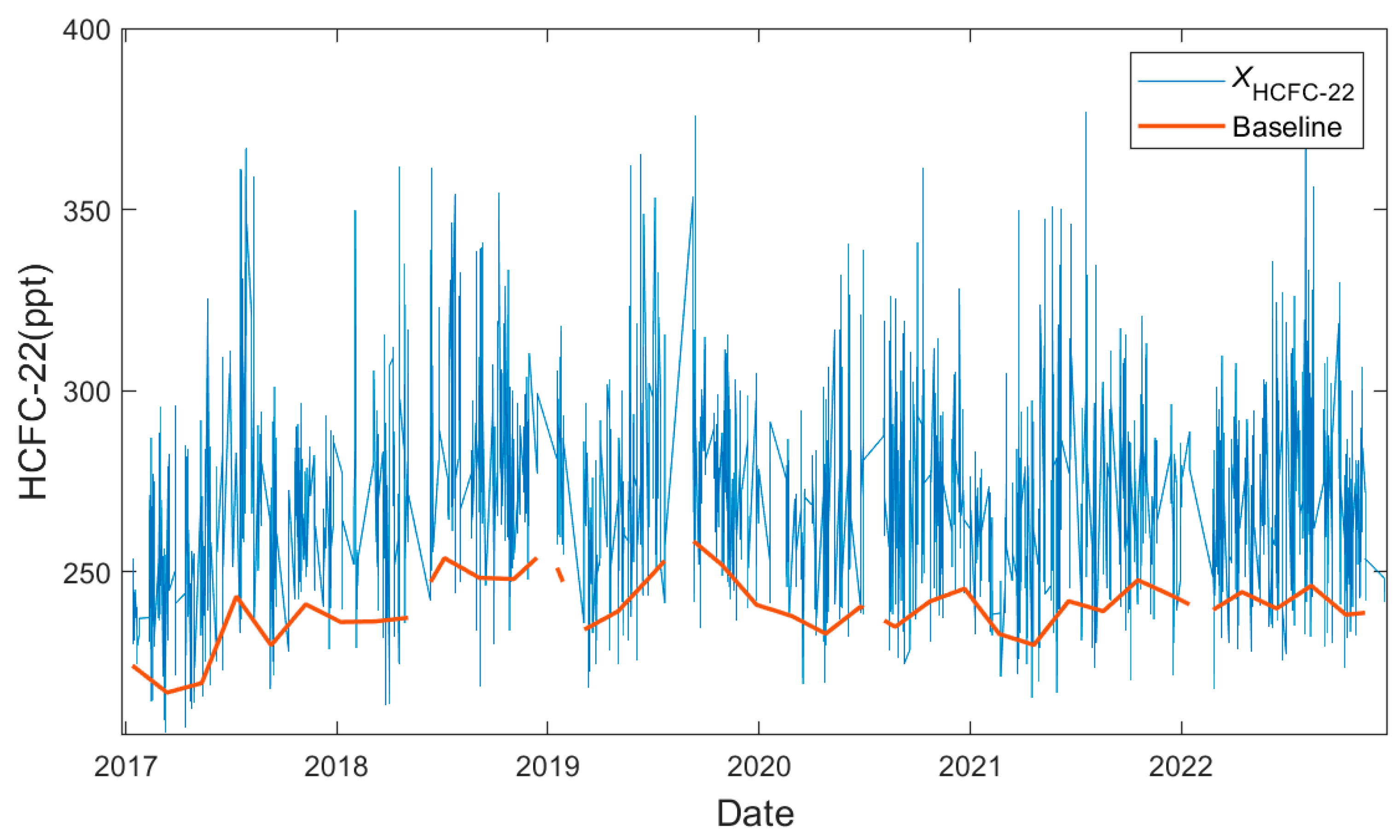
2.7. The Determination of the Baseline of the Dry Air Average Mole Fractions

The dry air average mole fraction ( X gas ) within a certain altitude range is calculated based on the HCFC-22 time series, as the input data for the emission calculation. The calculation formula is as follows [46]:
X gas = partial   column G partial   column dry air =   partial   column G   partial   column wet air partial   column H 2 O
where partial   column G , partial   column H 2 O , partial   column dry air , and partial   column wet air are the partial columns of the target gas, water vapor, dry air, and wet air, respectively. The calculation height range of X gas is set as 0–12 km, which is below the troposphere. Atmospheric pollutants are mainly transported and diffused within the troposphere, and spectral retrieval has a high sensitivity in the troposphere.
The optimal posterior estimation is made by minimizing the cost function J in the Bayesian inversion: the FLEXPART backward simulation only accounts for the concentration change at the observation station caused by emission transports in a period of time, while the baseline, namely, the background mole fraction of the target gas, needs to be additionally calculated in the Bayesian inversion calculation. The baseline value represents the contributions of all emissions in the past. We adopted the method described in Stohl (2009), which uses the measures X gas values and the simulated values, and the simulated values are based on a priori emission calculations [43]. Firstly, the lowest 25% of the observed values were selected during the 60-day moving time window, which are the values of those that are less affected by emissions. Then, the simulated concentration enhancements of the a priori emissions are calculated and subtracted from the selected observation values. Among them, the values above the median of the simulated mole fraction and the corresponding observation data are excluded to avoid overestimating the contribution of emissions. Finally, at each time window, the resulting values are averaged and linearly interpolated to the observation time. Figure 6 depicts the measured XHCFC-22 and the calculated baseline at the Hefei station.

3. Results

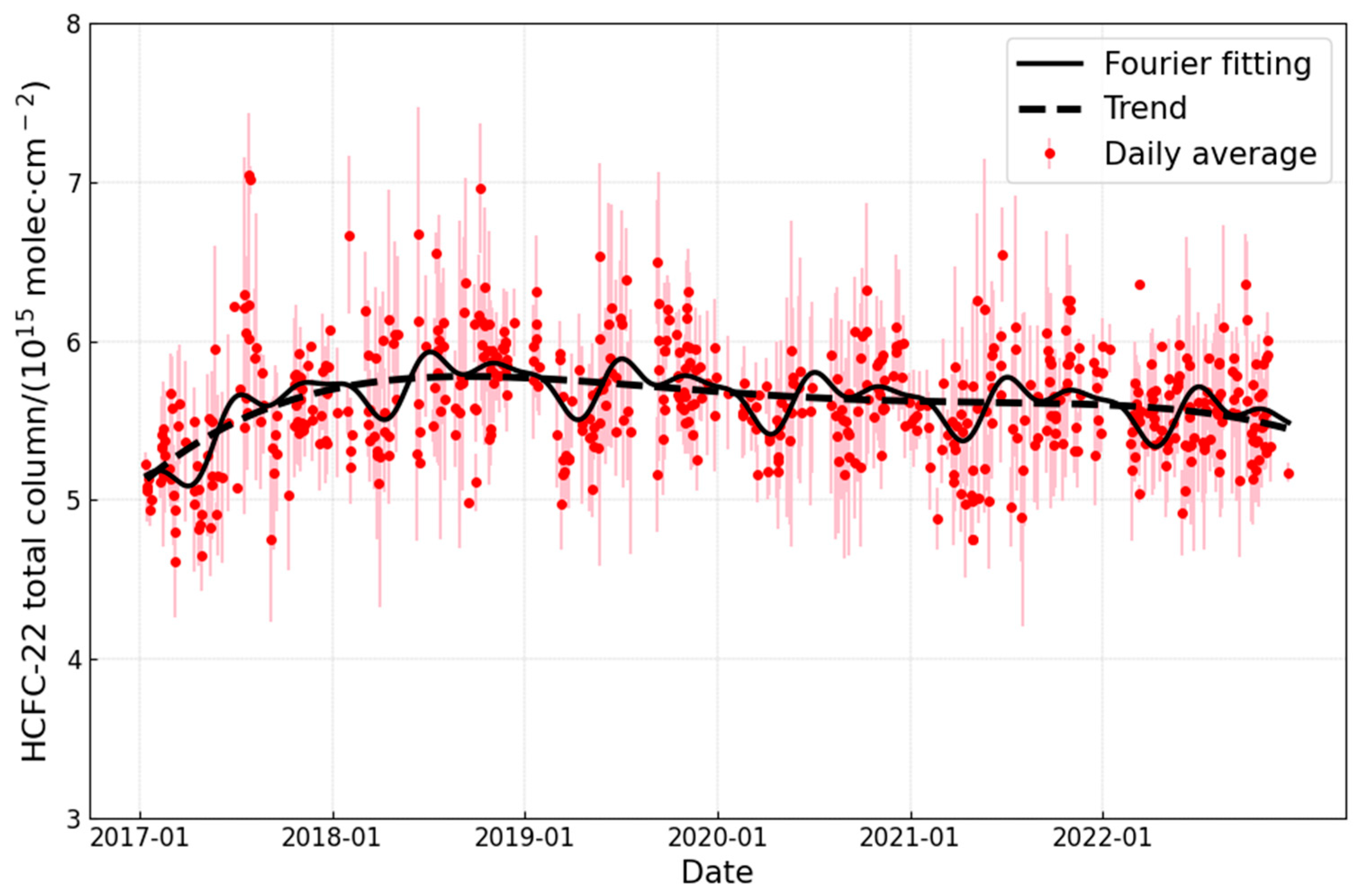
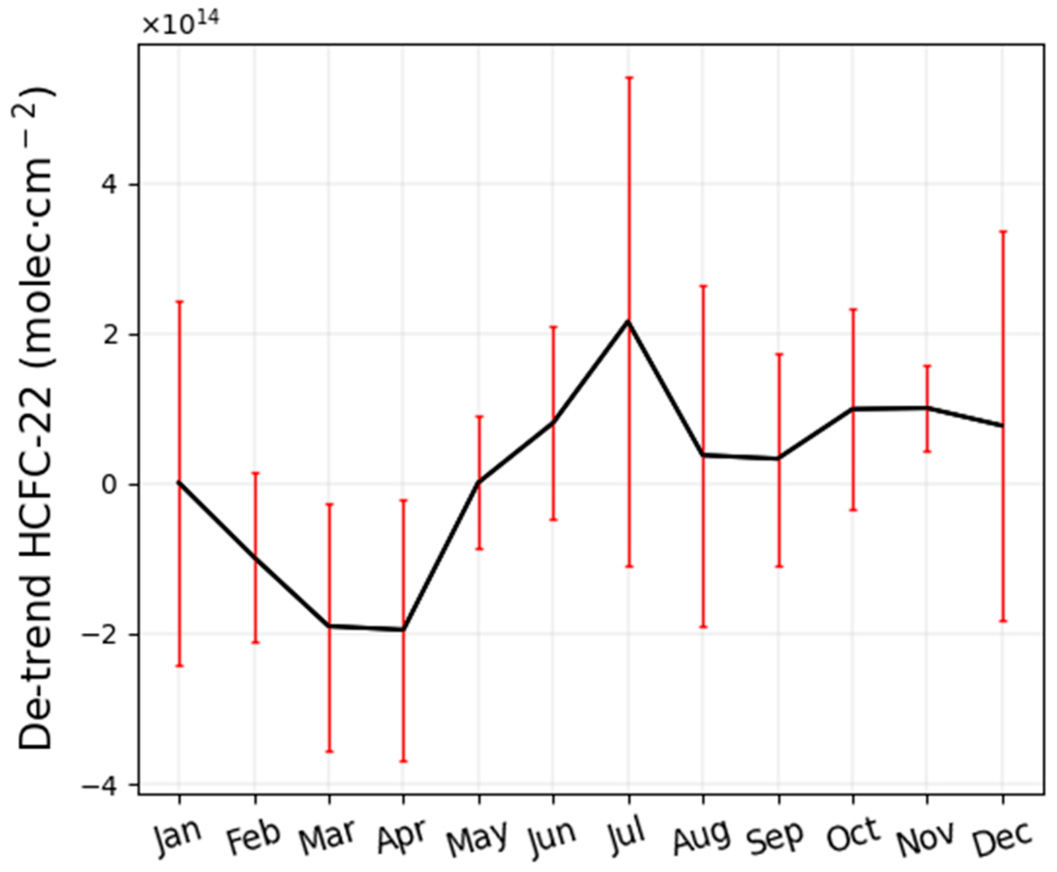
3.1. Annual Trend and Seasonal Cycle

The HCFC-22 data that exceed the mean ± 2σ for the RMS, systemic error, and random error were considered as outliers and discarded, and σ is the standard deviation. The seasonal variation and annual trend of HCFC-22’s total columns are simulated by polynomials and the Fourier series, and t is the year fraction:
F t = a + b · t + c · t 2 + d · t 3 + e · t 4 + k = 1 3 f 2 k 1 cos 2 π k t + f 2 k sin 2 π k t
a represents a constant; b , c , d , and e are polynomial coefficients with a fourth-order polynomial; and f 1 to f 6 represent sin/cosine harmonic term coefficients with third-order harmonic terms. Figure 7 shows the HCFC-22 data with Fourier and linearity fitting. The annual variation trend of HCFC-22’s total columns over Hefei shows an initial increase followed by a decrease from January 2017 to December 2022, as can be seen. The HCFC-22 total columns increased from 2017 to 2018, reached the peak in 2018 with an average annual value of approximately 5.74 × 10¹⁵ molec·cm−2, and gradually decreased from 2018 to 2022. The annual variation of the HCFC-22 total columns over Hefei is 5.98% from 2017 to 2018 and is −1.02 ± 0.01% from 2018 to 2022. According to the Montreal Protocol and the Kigali Amendment, China’s production and consumption of chlorofluorocarbons as refrigerants or foaming agents have started to freeze since 2013, achieving a 10% reduction in 2015 and a 35% reduction in 2020 [47]. The measured HCFC-22 columns above the Hefei atmosphere have decreased in recent years, indicating that the HCFC-22 decomposition rate is greater than the increase rate in emissions, and the policy of restricting production is effective. Yi et al. (2021) conducted in-situ measurements of major halocarbons in five Chinese cities and also demonstrated that the atmospheric concentration of HCFC-22 has shown a slowing down for the increase trend or a decreasing trend in recent years in China [48]. The time series at the St. Petersburg NADCC ground-based remote sensing station also have a similar variation trend compared with the Hefei station. Two stations applied the same remote sensing technology and retrieval algorithms to observe atmospheric HCFC-22. The HCFC-22 total columns over St. Petersburg slowly increased before 2016, then stabilized, and slightly decreased after 2017, with a growth rate of 1.19 ± 0.81% from 2013 to 2016 and −0.66 ± 0.49% from 2016 to 2019 [49]. Meanwhile, we also present the HCFC-22 annual trends obtained from other NDACC ground-based remote sensing stations and the ACE-FTS satellite (30°S–30°N) in Table 3.
We also obtained the average monthly variations of the HCFC-22 total columns at the Hefei station using de-trended data, which are shown in Figure 8, and which subtract the annual average. The HCFC-22 total columns show a clear seasonal variation, reaching the peak in July of the summer and the lowest point in April and March of the spring. The seasonal amplitude of HCFC-22, which is the monthly maximum minus the minimum values, is 4.10 × 10¹⁴ molec·cm−2. Then, the seasonal variability for the maximum and minimum months of HCFC-22 is 7% (seasonal amplitude/annual mean × 100%). Similar HCFC-22 seasonal variations also appear at Jungfraujoch in Switzerland and the Réunion Island station in the western Indian Ocean, with the highest value in the summer and the lowest value in the winter or spring [18,19]. The seasonal cycle measured at the stations is related to the seasonal cycle in emissions and atmospheric transport. As a common refrigerant, HCFC-22 is often used in the summer, and the high vapor pressure in refrigeration systems in the summer makes it easy to leak. Xiang et al. (2019) found that the summer HCFC-22 emissions are about two to three times the winter ones based on the aircraft data over the Pacific Ocean [50]. Chirkov et al. (2016) found that the HCFC-22 minimum value in the northern hemisphere during the spring may be related to the invasion of the stratospheric air lacking HCFC-22 at the end of the polar winter and during the breakdown of the polar vortex based on MIPAS satellite data [51]. Other tropospheric sources, such as CFCs, also reach the minimum in the spring at the Hefei station [52].

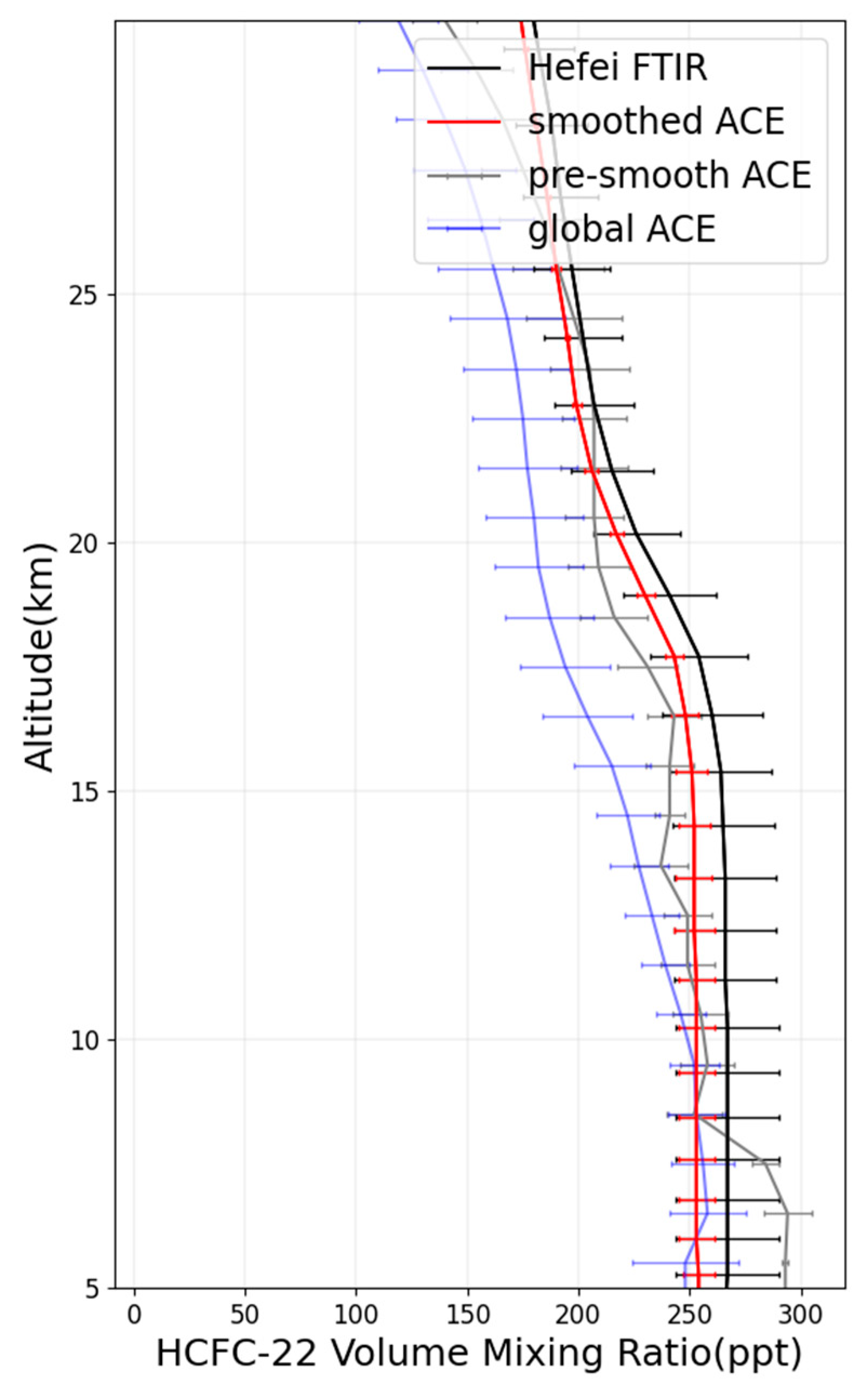
3.2. A Comparison with Satellite Data

Figure 9 plots FTIR profiles at the Hefei site, the 27–37° N and 107–127°E raw satellite profile, the smoothed satellite profile, and the global ACE-FTS satellite profile. We only compare the profiles at a 5–25 km altitude, as the main height range of the microwindow used by ACE-FTS for HCFC-22 is a 5–25 km altitude, and FTIR measurements also have a low sensitivity for HCFC-22’s retrieval above the 25 km altitude. As shown in Figure 9, the raw satellite profile at 27–37°N and 107–127°E is higher than the global ACE-FTS HCFC-22 measurements’ average profile, indicating that the HCFC-22 concentration near Hefei is relatively higher than the global average. The HCFC-22 vertical volume mixing ratio (VMR) profiles derive from the satellite at ±5° latitudes and ±10° longitudes centered on Hefei are relatively close to the profiles measured by the ground-based FTIR. The smoothed satellite VMR profiles are slightly lower than the VMR profiles observed by ground-based FTIR. The relative difference is calculated by subtracting the FTIR data from the smoothed satellite data and dividing them by FTIR data. Within the 5–25 km altitude range, the vertical relative difference between the satellite ACE-FTS database and FTIR data is −4.38 ± 0.83%. The HCFC-22 partial columns for the satellite data at the 5–25 km altitude range is 2.81 × 10¹⁵ molec·cm−2, and the partial columns for the FTIR data are 2.95 × 10¹⁵ molec·cm−2, with the partial column relative difference being −4.75%. The results indicate that the ground-based FTIR data at Hefei show good consistency with the ACE-FTS data for HCFC-22.

3.3. The Emission Estimations of HCFC-22 in the Yangtze River Delta

Table 4 lists the calculated emissions of HCFC-22 in the Yangtze River Delta in 2017–2022. In our study, the Yangtze River Delta’s HCFC-22 emissions peaked in 2017, with approximately 33.3 ± 16.8 kt, respectively. From 2018 to 2022, the HCFC-22 emissions in the Yangtze River Delta showed a downward trend, with a minimum value of 27.3 ± 13.6 kt in 2022. As can be seen, the emission values are close to the values determined by other methods, as in for example, the HCFC-22 emissions in 2017 and 2018 in the Yangtze River Delta, which used the interspecies correlation method by CO and HFC-134a [6]. Li estimated the HCFC-22 historical emissions from 1990 to 2014 and projected that HCFC-22 emissions would peak in 2016 under the legislative amendment in China [53]. Wu et al. obtained HCFC-22 emissions in various regions of China from 1990 to 2019 based on the bottom-up method and found that both the production and consumption of HCFC-22 had a peak in 2012 (364.6 and 165.0 kt, respectively), while the total emissions peaked in 2017 [4]. So, the variation trend of HCFC-22 emissions of the Yangtze River Delta are well consistent with that estimated by other studies. The Yangtze River Delta is an important source of HCFC-22 emissions in China, accounting for approximately 20% in the country’s total emissions [6]. The variation trend in emissions in this region reflects, to some extent, the variation in HCFC-22 in China.

4. Discussion

In our study, the atmospheric HCFC-22 total columns from January 2017 to December 2022 were retrieved based on ground-based high resolution FTIR infrared solar spectra measurements over Hefei, China. The annual trends and seasonal variations of atmospheric HCFC-22 were analyzed and compared with satellite data. Finally, the HCFC-22 emissions in the Yangtze River Delta from 2017–2022 were estimated based on the HCFC-22 total columns.
After using SFIT4 and the Tikhonov L 1 regularization to retrieve the HCFC-22 profile from mid-infrared spectra, it was found that the atmospheric HCFC-22 is distributed over the entire atmosphere, with high concentrations at 0–20 km. Based on the posteriori error estimation, the total retrieval error of HCFC-22 is 4.6%, including the systematic error, which is 3.8%, with the random error, which is 2.6%. Then, the HCFC-22 total columns over Hefei increased in 2017 and 2018, with an annual trend rate of 5.98%, and gradually decreased in 2018 to 2022, with a decrease rate of −1.02 ± 0.01%. The HCFC-22 total columns reached their peak in the summer (July) and had a lower peak in the spring (April). The seasonal amplitude between July and April is 4.10 × 10¹⁴ molec·cm−2. By a comparison of the Hefei retrievals with the satellite ACE-FTS database, the mean relative difference in the profiles is −4.38 ± 0.83% at 5 to 25 km. The HCFC-22 partial columns from the satellite observations are 2.81 × 10¹⁵ molec·cm−2 at 5–25 km, the partial columns from the FTIR measurements are 2.95 × 10¹⁵ molec·cm−2, and the relative difference is −4.75%.
Finally, the HCFC-22 dry air average mole fractions calculated using total columns were used to estimate the HCFC-22 emissions in the Yangtze River Delta region from 2017–2022, based on the atmospheric transport model FLEXPART and the Bayesian algorithm. The results show that the HCFC-22 emissions in the Yangtze River Delta were relatively high in 2017, with approximately 33.3 ± 16.8 kt. From 2018 to 2022, the HCFC-22 emissions decreased, with a minimum value of 27.3 ± 13.6 kt in 2022.

5. Conclusions

The atmospheric remote sensing measurement experiment based on ground-based FTIR at Hefei site showed the HCFC-22 over Hefei continued to decline after 2018. This is due to China’s recent HCFC-22 emission reduction policies, and the estimated HCFC-22 emissions in the Yangtze River Delta region have been declining since 2017. Although this study has regional limitations, it brings positive news for the reduction of atmospheric ozone depleting substances HCFC-22 and the restoration of the ozone layer.

Author Contributions

Resources, Y.X.; data curation, P.W., Q.Z. and B.L.; methodology—X.Z., W.W. and C.S.; writing—original draft preparation, X.Z.; visualization—Y.X.; writing—review and editing, W.W. and C.S.; funding acquisition, W.W. and C.L. All authors have read and agreed to the published version of the manuscript.

Funding

This research was supported by the National Key Technology R&D Program of China (2022YFB3904805), the National Natural Science Foundation of China (42305139), the Natural Science Foundation of Guangdong Province (2016A030310115), the Major Projects of High Resolution Earth Observation Systems of National Science and Technology (05-Y30B01-9001-19/20-3), the State Environmental Protection Key Laboratory of Sources and Control of Air Pollution Complex (No. SCAPC202110), the National Key Project for Causes and Control of Heavy Air Pollution (DQGG0102 and DQGG0205), the Strategic Priority Research Program of the Chinese Academy of Sciences (XDA23020301), and the National Key Technology R&D Program of China (2019YFC0214702).

Data Availability Statement

The FTIR HCFC-22 retrievals at Hefei are available by contacting the corresponding author.

Acknowledgments

We gratefully acknowledge Nicholas Jones, Wollongong University, for guidance on the spectroscopy retrievals. We are grateful to the NDACC networks for providing information and advice on the SFIT (version 0.9.4.4) software.

Conflicts of Interest

The authors declare no conflict of interest.

References

  1. Molina, M.J.; Rowland, F.S. Stratospheric Sink for Chlorofluoromethanes: Chlorine Atom-Catalysed Destruction of Ozone. Nature 1974, 249, 810–812. [Google Scholar] [CrossRef]
  2. Ko, M.; Newman, P.; Reimann, S.; Strahan, S.; Plumb, R.; Stolarski, R.; Burkholder, J.; Mellouki, W.; Engel, A.; Atlas, E. SPARC Report on Lifetimes of Stratospheric Ozone-Depleting Substances, Their Replacements, and Related Species. 2013, p. 256. Available online: www.sparc-climate.org/publications/sparc-reports/ (accessed on 1 March 2023).
  3. WMO (World Meteorological Organization). Scientific Assessment of Ozone Depletion: 2018; Report No. 58; Global Ozone Research and Monitoring Project: Geneva, Switzerland, 2018; p. 588. [Google Scholar]
  4. Wu, J.; Li, T.; Wang, J.; Zhang, D.Y.; Peng, L. Establishment of HCFC-22 National-Provincial-Gridded Emission Inventories in China and the Analysis of Emission Reduction Potential. Environ. Sci. Technol. 2022, 56, 814–822. [Google Scholar] [CrossRef] [PubMed]
  5. Fang, X.; Yao, B.; Vollmer, M.K.; Reimann, S.; Liu, L.; Chen, L.; Prinn, R.G.; Hu, J. Changes in HCFC Emissions in China during 2011–2017. Geophys. Res. Lett. 2019, 46, 10034–10042. [Google Scholar] [CrossRef]
  6. Yu, Y.; Xu, H.H.; Yao, B.; Pu, J.J.; Jiang, Y.J.; Ma, Q.L.; Fang, X.K.; O’Doherty, S.; Chen, L.Q.; He, J. Estimate of hydrochlorofluorocarbon emissions during 2011–2018 in the Yangtze River Delta, China. Environ. Pollut. 2022, 307, 119517. [Google Scholar] [CrossRef] [PubMed]
  7. An, X.; Henne, S.; Yao, B.; Vollmer, M.K.; Zhou, L.; Li, Y. Estimating emissions of HCFC-22 and CFC-11 in China by atmospheric observations and inverse modeling. Sci. China Chem. 2012, 55, 2233–2241. [Google Scholar] [CrossRef]
  8. Zhang, Y.; Wang, X.; Simpson, I.J.; Barletta, B.; Blake, D.R.; Meinardi, S.; Louie, P.K.K.; Zhao, X.; Shao, M.; Zhong, L.; et al. Ambient CFCs and HCFC-22 observed concurrently at 84 sites in the Pearl River Delta region during the 2008–2009 grid studies. J. Geophys. Res. Atmos. 2014, 119, 7699–7717. [Google Scholar] [CrossRef]
  9. Zhang, G.; Yao, B.; Vollmer, M.K.; Montzka, S.A.; Muhle, J.; Weiss, R.F.; O’Doherty, S.; Li, Y.; Fang, S.; Reimann, S. Ambient mixing ratios of atmospheric halogenated compounds at five background stations in China. Atmos. Environ. 2017, 160, 55–69. [Google Scholar] [CrossRef]
  10. Wetzel, G.; Hopfner, M.; Oelhaf, H.; Friedl-Vallon, F.; Kleinert, A.; Maucher, G.; Sinnhuber, M.; Abalichin, J.; Dehn, A.; Raspollini, P. Long-term validation of MIPAS ESA operational products using MIPAS-Bmeasurements. Atmos. Meas. Tech. 2022, 15, 6669–6704. [Google Scholar] [CrossRef]
  11. Moore, D.P.; Remedios, J.J. Growth rates of stratospheric HCFC-22. Atmos. Chem. Phys. 2008, 8, 73–82. [Google Scholar] [CrossRef]
  12. Cai, S.; Dudhia, A. Analysis of new species retrieved from MIPAS. Ann. Geophys. 2013, 56, 6340. [Google Scholar] [CrossRef]
  13. Nassar, R.; Bernath, P.F.; Boone, C.D.; McLeod, S.D.; Skelton, R.; Walker, K.A.; Rinsland, C.P.; Duchatelet, P. A global inventory of stratospheric fluorine in 2004 based on Atmospheric Chemistry Experiment Fourier transform spectrometer (ACE-FTS) measurements. J. Geophys. Res. Atmos. 2006, 111, D22313. [Google Scholar] [CrossRef]
  14. Nassar, R.; Bernath, P.F.; Boone, C.D.; Clerbaux, C.; Coheur, P.F.; Dufour, G.; Froidevaux, L.; Mahieu, E.; McConnell, J.C.; McLeod, S.D.; et al. A global inventory of stratospheric chlorine in 2004. J. Geophys. Res. Atmos. 2006, 111, D22312. [Google Scholar] [CrossRef]
  15. Brown, A.T.; Chipperfield, M.P.; Boone, C.; Wilson, C.; Walker, K.A.; Bernath, P.F. Trends in atmospheric halogen containing gases since 2004. J. Quant. Spectrosc. Radiat. Transf. 2011, 112, 2552–2566. [Google Scholar] [CrossRef]
  16. Chen, A.; Chen, D.; Hu, X.Y.; Harth, C.M.; Young, D.; Muhle, J.; Krummel, P.B.; O’Doherty, S.; Weiss, R.F.; Prinn, R.G.; et al. Historical trend of ozone-depleting substances and hydrofluorocarbon concentrations during 2004–2020 derived from satellite observations and estimates for global emissions. Environ. Pollut. 2023, 316, 120570. [Google Scholar] [CrossRef]
  17. Steffen, J.; Bernath, P.F.; Boone, C.D. Trends in halogen-containing molecules measured by the Atmospheric Chemistry Experiment (ACE) satellite. J. Quant. Spectrosc. Radiat. Transf. 2019, 238, 106619. [Google Scholar] [CrossRef]
  18. Zhou, M.Q.; Vigouroux, C.; Langerock, B.; Wang, P.; Dutton, G.; Hermans, C.; Kumps, N.; Metzger, J.M.; Toon, G.; De Maziere, M. CFC-11, CFC-12 and HCFC-22 ground-based remote sensing FTIR measurements at Reunion Island and comparisons with MIPAS/ENVISAT data. Atmos. Meas. Tech. 2016, 9, 5621–5636. [Google Scholar] [CrossRef]
  19. Prignon, M.; Chabrillat, S.; Minganti, D.; O’Doherty, S.; Seryais, C.; Stiller, G.; Toon, G.C.; Vollmer, M.K.; Mahieu, E. Improved FTIR retrieval strategy for HCFC-22 (CHClF2), comparisons with in situ and satellite datasets with the support of models, and determination of its long-term trend above Jungfraujoch. Atmos. Chem. Phys. 2019, 19, 12309–12324. [Google Scholar] [CrossRef]
  20. Polyakov, A.; Poberovsky, A.; Makarova, M.; Virolainen, Y.; Timofeyev, Y.; Nikulina, A. Measurements of CFC-11, CFC-12, and HCFC-22 total columns in the atmosphere at the St. Petersburg site in 2009–2019. Atmos. Meas. Tech. 2021, 14, 5349–5368. [Google Scholar] [CrossRef]
  21. National Development and Reform Commission. Available online: https://www.ndrc.gov.cn/xxgk/jd/wsdwhfz/202008/t20200803_1235430.html (accessed on 20 September 2023).
  22. National Development and Reform Commission. List of Relevant Third-Party Verification Agencies and HCFC-22 Manufacturers. 2018. Available online: https://www.ndrc.gov.cn/xxgk/zcfb/tz/201803/W020190905503776929718.pdf (accessed on 1 March 2023).
  23. Bruker FT-IR Spectrometer IFS 125HR. Available online: https://www.bruker.com/en/products-and-solutions/infrared-and-raman/ft-ir-research-spectrometers/ifs-125hr-high-resolution-ft-ir-spectrometer.html (accessed on 24 November 2023).
  24. Coastal Environmental System ZENO-3200. Available online: https://s.campbellsci.com/documents/us/manuals/zeno-3200-manual.pdf (accessed on 24 November 2023).
  25. Wang, W.; Tian, Y.; Liu, C.; Sun, Y.; Liu, W.; Xie, P.; Liu, J.; Xu, J.; Morino, I.; Velazco, V.A.; et al. Investigating the performance of a greenhouse gas observatory in Hefei, China. Atmos. Meas. Tech. 2017, 10, 2627–2643. [Google Scholar] [CrossRef]
  26. Shan, C.; Zhang, H.; Wang, W.; Liu, C.; Xie, Y.; Hu, Q.; Jones, N. Retrieval of Stratospheric HNO3 and HCl Based on Ground-Based High-Resolution Fourier Transform Spectroscopy. Remote Sens. 2021, 13, 2159. [Google Scholar] [CrossRef]
  27. Wu, P.; Shan, C.; Liu, C.; Xie, Y.; Wang, W.; Zhu, Q.; Zeng, X.; Liang, B. Ground-Based Remote Sensing of Atmospheric Water Vapor Using High-Resolution FTIR Spectrometry. Remote Sens. 2023, 15, 3484. [Google Scholar] [CrossRef]
  28. Yin, H.; Sun, Y.; Song, Z.; Liu, C.; Wang, W.; Shan, C.; Zha, L. Remote Sensing of Atmospheric Hydrogen Fluoride (HF) over Hefei, China with Ground-Based High-Resolution Fourier Transform Infrared (FTIR) Spectrometry. Remote Sens. 2021, 13, 791. [Google Scholar] [CrossRef]
  29. NASA Jet Propulsion Laboratory. Available online: http://mark4sun.jpl.nasa.gov/pseudo.html (accessed on 5 March 2023).
  30. Kalnay, E.; Kanamitsu, M.; Kistler, R.; Collins, W.; Deaven, D.; Gandin, L.; Iredell, M.; Saha, S.; White, G.; Woollen, J.; et al. The NCEP/NCAR 40-year reanalysis project. Bull. Am. Meteorol. Soc. 1996, 77, 437–471. [Google Scholar] [CrossRef]
  31. IRWG-NDACC: WACCM V.6 Profiles Dataset for IRWG Sites, NDACC Infrared Working Group [Data Set]. Available online: ftp://nitrogen.acom.ucar.edu/user/jamesw/IRWG/2013/WACCM/V6 (accessed on 10 June 2023).
  32. Rodgers, C.D. Inverse Methods for Atmospheric Sounding: Theory and Practice, Oceanic and Planetary Physics; World Scientific: Singapore, 2000; Volume 2. [Google Scholar]
  33. Tikhonov, A.N. On the Solution of Incorrectly Stated Problems and a Method of Regularization. In Doklady Akademii Nauk; SSSR: Moscow, Russia, 1963. [Google Scholar]
  34. Sussmann, R.; Forster, F.; Rettinger, M.; Jones, N. Strategy for high-accuracy-and-precision retrieval of atmospheric methane from the mid-infrared FTIR network. Atmos. Meas. Tech. 2011, 4, 1943–1964. [Google Scholar] [CrossRef]
  35. Rodgers, C.D.; Connor, B.J. Intercomparison of remote sounding instruments. J. Geophys. Res. Atmos. 2003, 108. [Google Scholar] [CrossRef]
  36. Bernath, P. Atmospheric Chemistry Experiment (ACE): An overview. In Proceedings of the Conference on Earth Observing Systems VII, Seattle, WA, USA, 7–10 July 2002; pp. 39–49. [Google Scholar]
  37. De Maziere, M.; Vigouroux, C.; Bernath, P.F.; Baron, P.; Blumenstock, T.; Boone, C.; Brogniez, C.; Catoire, V.; Coffey, M.; Duchatelet, P.; et al. Validation of ACE-FTS v2.2 methane profiles from the upper troposphere to the lower mesosphere. Atmos. Chem. Phys. 2008, 8, 2421–2435. [Google Scholar] [CrossRef]
  38. Zhou, M.; Langerock, B.; Vigouroux, C.; Wang, P.; Hermans, C.; Stiller, G.; Walker, K.A.; Dutton, G.; Mahieu, E.; De Maziere, M. Ground-based FTIR retrievals of SF6 on Reunion Island. Atmos. Meas. Tech. 2018, 11, 651–662. [Google Scholar] [CrossRef]
  39. Seibert, P.; Frank, A. Source-receptor matrix calculation with a Lagrangian particle dispersion model in backward mode. Atmos. Chem. Phys. 2004, 4, 51–63. [Google Scholar] [CrossRef]
  40. Pisso, I.; Sollum, E.; Grythe, H.; Kristiansen, N.I.; Cassiani, M.; Eckhardt, S.; Arnold, D.; Morton, D.; Thompson, R.L.; Zwaaftink, C.D.G.; et al. The Lagrangian particle dispersion model FLEXPART version 10.4. Geosci. Model Dev. 2019, 12, 4955–4997. [Google Scholar] [CrossRef]
  41. Stohl, A.; Hittenberger, M.; Wotawa, G. Validation of the Lagrangian particle dispersion model FLEXPART against large-scale tracer experiment data. Atmos. Environ. 1998, 32, 4245–4264. [Google Scholar] [CrossRef]
  42. Henne, S.; Brunner, D.; Oney, B.; Leuenberger, M.; Eugster, W.; Bamberger, I.; Meinhardt, F.; Steinbacher, M.; Emmenegger, L. Validation of the Swiss methane emission inventory by atmospheric observations and inverse modelling. Atmos. Chem. Phys. 2016, 16, 3683–3710. [Google Scholar] [CrossRef]
  43. Stohl, A.; Seibert, P.; Arduini, J.; Eckhardt, S.; Fraser, P.; Greally, B.R.; Lunder, C.; Maione, M.; Muehle, J.; O’Doherty, S.; et al. An analytical inversion method for determining regional and global emissions of greenhouse gases: Sensitivity studies and application to halocarbons. Atmos. Chem. Phys. 2009, 9, 1597–1620. [Google Scholar] [CrossRef]
  44. Fang, X.K.; Ravishankara, A.R.; Velders, G.J.M.; Molina, M.J.; Su, S.S.; Zhang, J.B.; Hu, J.X.; Prinn, R.G. Changes in Emissions of Ozone-Depleting Substances from China Due to Implementation of the Montreal Protocol. Environ. Sci. Technol. 2018, 52, 11359–11366. [Google Scholar] [CrossRef]
  45. Gridded Population of the World (GPW) Version 4. Available online: https://sedac.ciesin.columbia.edu/data/collection/gpw-v4 (accessed on 1 June 2023).
  46. Zhou, M.Q.; Langerock, B.; Vigouroux, C.; Sha, M.K.; Ramonet, M.; Delmotte, M.; Mahieu, E.; Bader, W.; Hermans, C.; Kumps, N.; et al. Atmospheric CO and CH4 time series and seasonal variations on Reunion Island from ground-based in situ and FTIR (NDACC and TCCON) measurements. Atmos. Chem. Phys. 2018, 18, 13881–13901. [Google Scholar] [CrossRef]
  47. Ministry of Ecology and Environment of the People’s Republic of China. Available online: https://www.mee.gov.cn/ywdt/zbft/202306/t20230615_1033878.shtml (accessed on 20 June 2023).
  48. Yi, L.; Wu, J.; An, M.; Xu, W.; Fang, X.; Yao, B.; Li, Y.; Gao, D.; Zhao, X.; Hu, J. The atmospheric concentrations and emissions of major halocarbons in China during 2009–2019 *. Environ. Pollut. 2021, 284. [Google Scholar] [CrossRef] [PubMed]
  49. Polyakov, A.; Virolainen, Y.; Poberovskiy, A.; Makarova, M.; Timofeyev, Y. Atmospheric HCFC-22 total columns near St. Petersburg: Stabilization with start of a decrease. Int. J. Remote Sens. 2020, 41, 4365–4371. [Google Scholar] [CrossRef]
  50. Xiang, B.; Patra, P.K.; Montzka, S.A.; Miller, S.M.; Elkins, J.W.; Moore, F.L.; Atlas, E.L.; Miller, B.R.; Weiss, R.F.; Prinn, R.G.; et al. Global emissions of refrigerants HCFC-22 and HFC-134a: Unforeseen seasonal contributions. Proc. Natl. Acad. Sci. USA 2014, 111, 17379–17384. [Google Scholar] [CrossRef] [PubMed]
  51. Chirkov, M.; Stiller, G.P.; Laeng, A.; Kellmann, S.; von Clarmann, T.; Boone, C.D.; Elkins, J.W.; Engel, A.; Glatthor, N.; Grabowski, U.; et al. Global HCFC-22 measurements with MIPAS: Retrieval, validation, global distribution and its evolution over 2005–2012. Atmos. Chem. Phys. 2016, 16, 3345–3368. [Google Scholar] [CrossRef]
  52. Zeng, X.; Wang, W.; Liu, C.; Shan, C.; Xie, Y.; Wu, P.; Zhu, Q.; Zhou, M.; De Maziere, M.; Mahieu, E.; et al. Retrieval of atmospheric CFC-11 and CFC-12 from high-resolution FTIRobservations at Hefei and comparisons with other independent datasets. Atmos. Meas. Tech. 2022, 15, 6739–6754. [Google Scholar] [CrossRef]
  53. Li, Z.F.; Bie, P.J.; Wang, Z.Y.; Zhang, Z.Y.; Jiang, H.Y.; Xu, W.G.; Zhang, J.B.; Hu, J.X. Estimated HCFC-22 emissions for 1990–2050 in China and the increasing contribution to global emissions. Atmos. Environ. 2016, 132, 77–84. [Google Scholar] [CrossRef]
Figure 1. (a) Ground-based high-resolution FTIR spectrometer; (b) Solar tracker (A547).
Remotesensing 15 05590 g001
Figure 2. The typical spectrum of measured (blue) and fitted (red) HCFC-22 (CHF2Cl) (02:45:14 UTC 2 January 2022, solar zenith angle of 58.69°).
Remotesensing 15 05590 g002
Figure 3. The HCFC-22 profiles, including an a priori profile and a retrieved profile.
Remotesensing 15 05590 g003
Figure 4. The HCFC-22 typical averaging kernels.
Remotesensing 15 05590 g004
Figure 5. The emission sensitivity of the backward trajectory simulated by FLEXPART from 2017 to 2022. The Hefei station is the black dot, and the black box indicates the Yangtze River Delta.
Remotesensing 15 05590 g005
Figure 6. The atmospheric XHCFC-22 time series (blue) and the baseline (orange) measured at Hefei.
Remotesensing 15 05590 g006
Figure 7. Time series of HCFC-22 total columns measured at Hefei site. The red dots are HCFC-22 daily averages. The light red error bar is the daily standard deviation. The black solid and dashed lines are the Fourier series and the fourth-order polynomial linearity fitting curves, respectively.
Remotesensing 15 05590 g007
Figure 8. The monthly average of the de-trended total columns for HCFC-22. The black line represents the monthly variation, and the red line represents the error bar.
Remotesensing 15 05590 g008
Figure 9. The HCFC-22 vertical profiles. The ground-based FTIR profile is black, the ACE-FTS satellite, before smoothing (27–37°N and 107–127°E), is grey, the global ACE-FTS satellite profile is blue, and the smoothed ACE-FTS satellite profile (27–37°N and 107–127°E) is red.
Remotesensing 15 05590 g009
Table 1. Retrieval parameters used for HCFC-22.
SpeciesHCFC-22
microwindow828.75–829.4
Interfering speciesH2O, CO2, O3
SpectroscopyPLL, HITRAN 2012
T, P and H2O profilesNCEP
A priori profileWACCAM v6
Table 2. Error budgets for the HCFC-22 retrievals at Hefei.
ParameterUncertainty/%Systematic Error/%Random Error/%
Smoothing -0.84-
Measurement--2.49
Retrieval -0.04-
Interfering species-0.55-
Temperature-0.110.68
SZA0.1/0.20.070.14
Line intensity51.26-
Line T broadening52.00-
Line P broadening50.86-
H2O spectroscopy102.57-
ILS20.050.05
zshift10.390.39
Total-3.82.6
Table 3. The atmospheric HCFC-22 annual trends at Hefei and other ground-based remote sensing sites, namely, St. Petersburg, Réunion Island, Jungfraujoch, and the satellite ACE-FTS (30°S–30°N).
DataPeriodTrend (% Year−1)
Hefei2017–20185.98
2018–2022−1.02 ± 0.01
St. Petersburg [49]2013–20161.19 ± 0.81
2016–2019−0.66 ± 0.49
Réunion Island [18]2004–20162.84 ± 0.06
Jungfraujoch [19]2012–20171.72 ± 0.31
ACE-FTS (30°S–30°N) [17]2012–20181.74 ± 0.08
Table 4. A priori emissions and estimations of HCFC-22 emissions in the Yangtze River Delta, 1 sigma uncertainty.
PeriodA Priori Emissions (China)
(kt/Year) [44]
This Study
(kt/Year)
Emissions by CO Interspecies
Correlation (kt/Year) [6]
Emissions by
HFC-134a Interspecies Correlation (kt/Year) [6]
2017167.533.3 ± 16.829.8 ± 15.630.8 ± 10.5
2018165.232.6 ± 16.331.6 ± 17.9
2019161.031.9 ± 16.0
2020155.630.7 ± 15.4
2021148.429.2 ± 14.6
2022138.927.3 ± 13.6
Disclaimer/Publisher’s Note: The statements, opinions and data contained in all publications are solely those of the individual author(s) and contributor(s) and not of MDPI and/or the editor(s). MDPI and/or the editor(s) disclaim responsibility for any injury to people or property resulting from any ideas, methods, instructions or products referred to in the content.

