1. Introduction
Tropical cyclones (TCs) continue to rank among the most destructive of natural hazards, representing a threat to life and property stemming from associated phenomena of high winds, storm surge flooding, and heavy rainfall [
1]. For example, the National Oceanic and Atmospheric Administration (NOAA) estimates that of the total damage costs due to billion-dollar-magnitude weather-related disasters in the U.S. during the 1980–2023 period, more than 50 percent—or
$1.368 trillion—were due to TC events. Additionally, TCs accounted for nearly half, or 6895, of all such weather-related fatalities [
2]. In 2022, the US experienced its third most costly year, with damage totaling nearly
$178 billion. Of this, a record
$119 billion in damage was due to TC events [
2]. Effective mitigation of the financial and societal costs of such storms depends on timely warnings to the public across a range of timescales, from hours to days. Various factors influence the intensity of a TC, including ocean water temperatures, atmospheric pressure, temperature, and water vapor [
3]. Previous research has highlighted the importance of the eyewall, an area identified as a key focus for research due to its association with the hurricane’s most powerful winds [
4]. The surface pressure decreases and water temperatures rise through the eyewall and into the eye center, the latter acting as a rotation axis for the rest of the storm [
5]. Therefore, accurate and timely estimations of TC intensity are crucial for monitoring and predicting TC characterization, helping to prevent damage to life and property.
The characterization and prediction of TCs are based mainly on accurate observations of the storm’s 3-dimensional structure (e.g., temperature, water vapor, horizontal winds, surface pressure, and hydrometeors) and subsequent forecasts using numerical prediction models. While satellite observations offer the advantages of near-global coverage and remote measurement, the estimation of TC structure and intensity remains a difficult problem, and direct in situ measurements of atmospheric temperature, water vapor, and wind via instrumented aircraft and deployed dropsondes are still considered the most accurate of the available data. However, given the occurrence of TCs in multiple ocean basins worldwide and the costs associated with dedicated aircraft missions, not all TCs can be directly sampled, and remote satellite-based methods may be the only source of information on TC structure in many parts of the world. Remote observations from a range of satellite-borne instruments, including visible, infrared, and microwave sensors, have found widespread application to TC characterization, including intensity. Satellite passive microwave observations can often provide unique critical information on TC structure as microwave observations can penetrate in and through non-precipitating cloud systems, but the TC environment is also challenging for a number of reasons: Extreme values of wind speed and surface pressure occurring at small spatial scales, along with the presence of hydrometeors, could potentially limit the information on storm intensity in the microwave observations and further affect the prediction accuracy of TC intensity surrounding the eyewall using traditional methods. A standard measure of hurricane intensity is its maximum sustained wind speed. A typical inverse relationship to the maximum sustained wind speed is the minimum surface pressure at the hurricane center. These two variables are the focal point of tropical cyclone intensity estimation in this study.
Among the most well-established methods of TC intensity estimation is the Dvorak technique. Variations of the Dvorak technique [
6] have been widely used at operational forecast centers worldwide to estimate TC intensity. Since its original development in the 1970s as a subjective technique that used cyclone and cloud pattern classification approaches, the method has seen numerous updates with the goal of eliminating the subjectivity of its estimates, which can lead to inconsistencies in intensity estimates between ocean basins. Originally limited to infrared satellite measurements, recent updates have included passive microwave observations, mainly to address known limitations during TC intensification in cases where the hurricane eyewall may be obscured by high-level clouds. In terms of passive microwave measurements, there is a large body of work on characterizing TCs from space-borne microwave radiometers such as the Advanced Microwave Sounding Unit (AMSU-A), the Microwave Humidity Sounder (MHS), and the Advanced Technology Microwave Sounder (ATMS) [
7,
8,
9]. Much of this work has focused on the warm core feature and linking it to TC intensity [
10,
11,
12,
13,
14]. A direct estimation of surface wind speed using microwave observations was demonstrated in Hong et al. [
15]. That study utilized conically-scanning AMSR-2 measurements at 6.9 GHz combined with regression-based estimates of ocean surface reflectivity and small-scale roughness to determine wind speed. Results under rainy and non-rainy conditions showed a root mean squared error (RMSE) of 1.6 m/s when matched with in-situ buoy measurements. As previously indicated, the accuracy of traditional methods was limited by the information on storm intensity available from microwave observations. Additionally, these methods overlooked the effects of the surrounding areas of TCs.
Artificial intelligence (AI) and machine learning (ML)-based approaches have been applied to a wide range of geophysical problems and have shown great potential. Given the time constraints for intensity estimation associated with operational forecast environments, AI/ML applications offer an efficient and potentially powerful set of tools to produce timely and valuable information for both forecasters and researchers.
For example, Chen et al. [
16] developed a convolutional neural network (CNN) applied to satellite infrared imagery to estimate TC intensity (wind speed). When compared to the best track analysis data, a RMSE of 4.3 m/s was reported. Tian et al. [
17] used deep learning models combined with infrared, water vapor, visible, and passive microwave measurements and obtained RMSE differences with independent measurements of 4.2 m/s. Wimmers et al. [
18] implemented a CNN approach applied to conically-scanning passive microwave observations to estimate wind speed and reported RMSE differences with operational best track data of 7.3 m/s.
In comparison to traditional methods, AI applications in TC intensity have demonstrated a clear advantage in efficiency. Furthermore, the CNN was capable of predicting conditions in areas surrounding the TCs rather than a single point, effectively accounting for the interactions among adjoint points. Therefore, in this study, we apply a deep learning approach to passive microwave measurements from the cross-track scanning ATMS instrument. A U-Net machine learning algorithm was developed to predict surface wind speed and surface pressure surrounding TCs and to further extract those parameters from the eyewall of TCs. An explanation of the U-Net model is presented in
Section 2, followed by an overview of the data in
Section 3. In
Section 4, the results of the wind speed and surface pressure predictions will be discussed.
Section 5—the discussion section—highlights the specifics of this research and the advantages of using the U-Net algorithm in this study, followed by conclusions and avenues for future work in
Section 6.
2. Methodology
U-Net, the evolution of the traditional convolutional neural network (CNN) algorithm, was designed to train using fewer images to produce more precise image segmentations [
19]. U-Nets have many similarities with a conventional encoder-decoder CNN: a contracting path (i.e., encoder), spatial filtering layers, pooling layers, a corresponding expansive path (i.e., decoder), and, optionally, one or more fully connected layers. For image-like data, CNNs have some advantages compared with traditional, fully connected neural networks. For example, the use of 2-dimensional convolutional filters allows for local feature extraction and an accounting of spatial relationships in the data. Also, only a single set of weights and biases is determined for the entire processing domain for each convolutional filter, which can significantly reduce the number of parameters that need to be determined during the training phase. The U-Net differs from a typical CNN encoder-decoder in the expansive path, where each expansive layer is supplemented (concatenated) with higher-resolution information (feature maps) obtained from the corresponding layer in the contracting path. This allows the U-Net to preserve more high-resolution information in the final output prediction than would be obtained from a conventional encoder-decoder CNN.
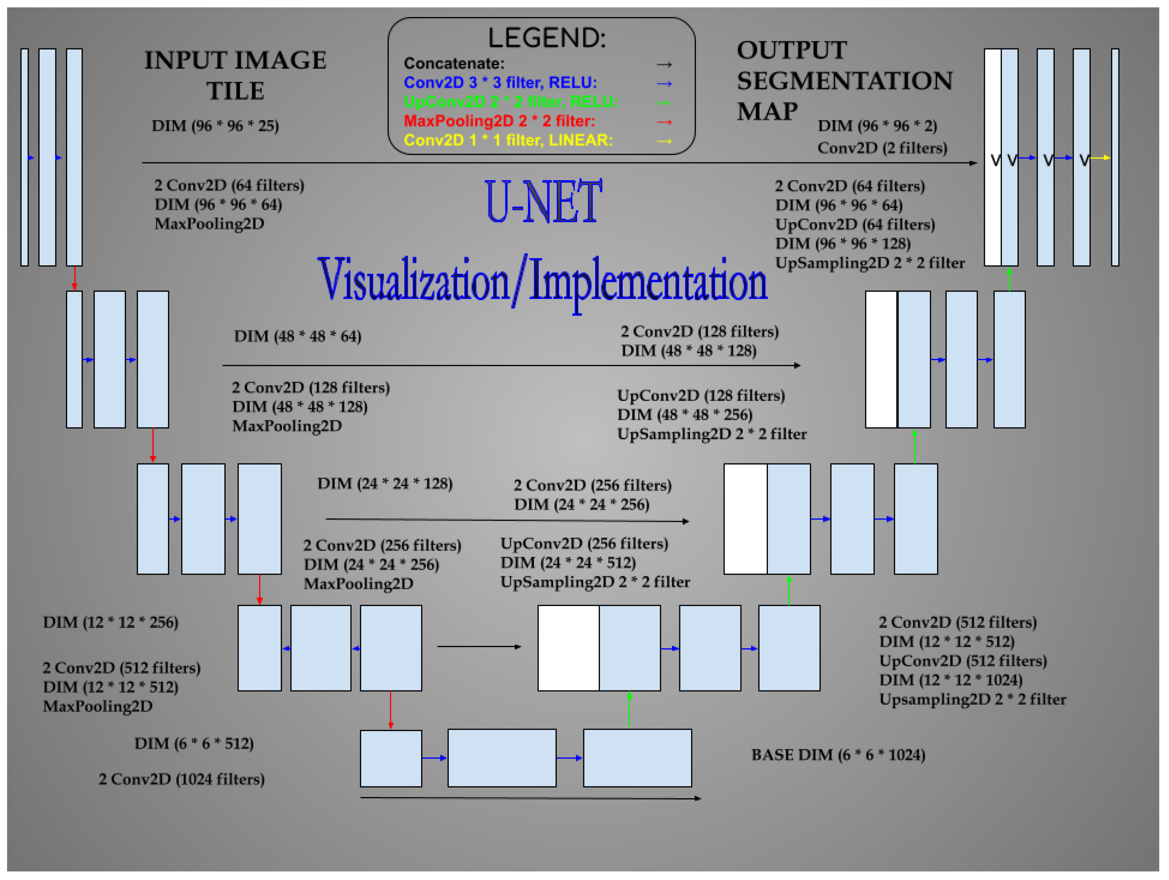
The architecture of the U-Net in this study is illustrated in
Figure 1. The U-Net follows a symmetric U shape divided into two paths leading down and up the network, called the contracting path and the expansive path. A total of 23 convolutional layers were employed. In the contracting path, the network undergoes a series of convolutional processes across five levels. Each level comprises two Conv2D layers with 3 × 3 filters, followed by a Max Pooling layer with 2 × 2 filters, constituting a total of 10 convolutional layers. This path effectively reduces the spatial dimensions of the image while increasing the number of channels. The fifth level serves as the bridge between the contracting and expansive paths. As the network transitions to the expansive path, it undergoes expansion through upsampling, which doubles the dimensions of the image while halving the number of feature channels at each of the four levels. This process, known as up-convolution [
19], is followed by the concatenation of the upscaled feature map with its corresponding feature map from the contracting path, reintegrating spatial information lost during downsampling. After concatenation, two Conv2D layers with 3 × 3 filters and rectified linear unit (ReLU) activation are applied at each level of expansion, contributing to a total of 12 convolutional layers in the expansive path. A final convolutional layer with 1 × 1 filters is used to map each 64-component feature vector to the desired number of classes, resulting in 23 convolutional layers for the entire network. This design is consistent with the original U-Net architecture [
19]. However, in the original U-Net design, the SoftMax activation function was commonly used in the final layer. SoftMax is a mathematical function that converts a vector of numerical values into a vector of probabilities, with each value representing the probability that the input belongs to one of the classes. This function is particularly useful in multi-class classification problems where each class is mutually exclusive [
20]. On the other hand, in the case of TC intensity, the objective is to forecast a continuous numerical value representing the intensity rather than categorizing it into distinct classes, hence a regression problem. Therefore, the employment of a linear activation function in the last layer of the U-Net model was more suitable for this study.
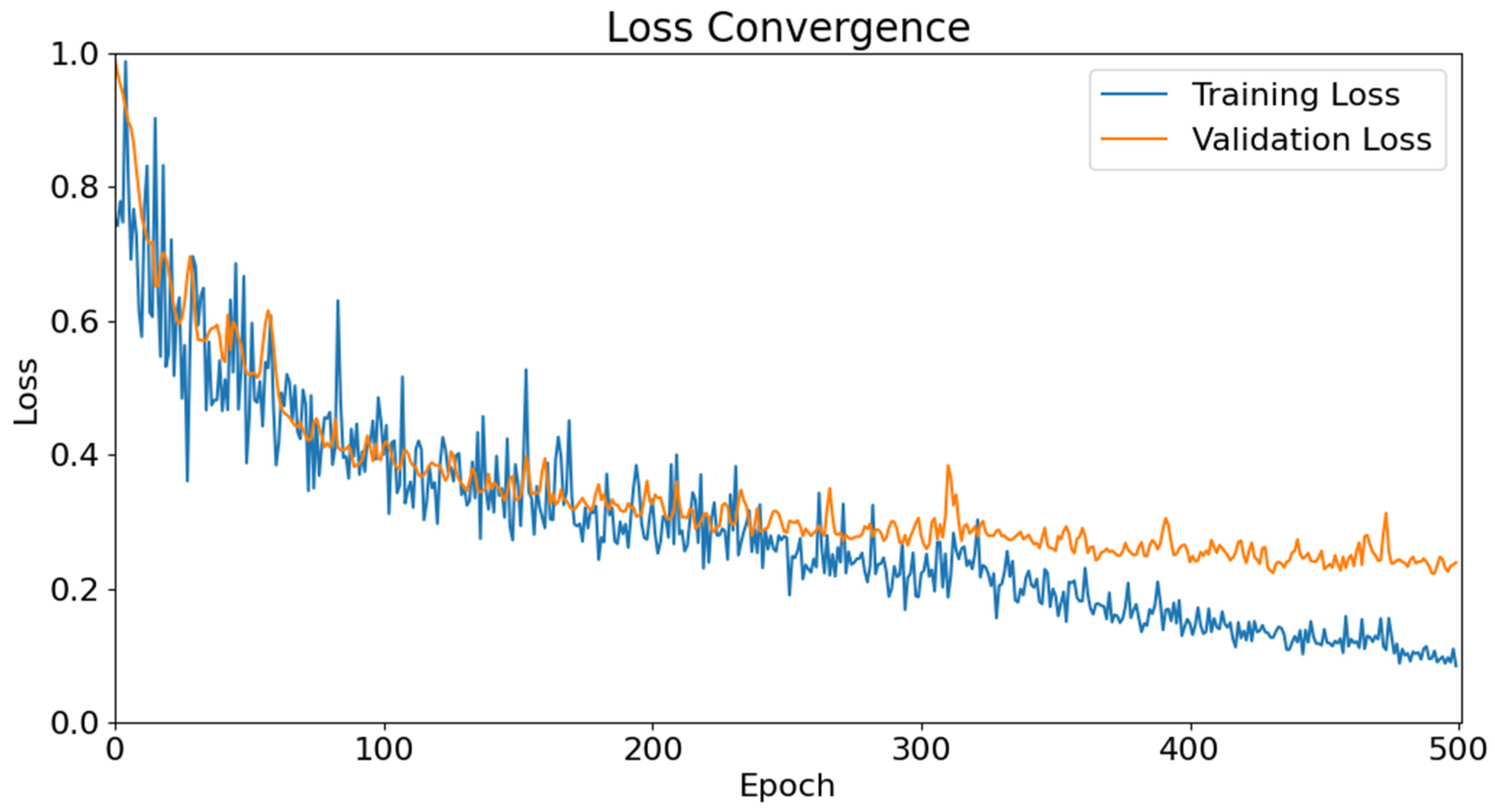
Training the model requires tuning standard deep learning hyperparameters. The learning rate controls the step size at which the model converges. A higher learning rate contributes to a quicker model learning process. However, it is possible that a learning rate too large could overshoot the global minimum and diverge. Thus, a lower learning rate gives a better chance of converging to the global minimum, but some drawbacks of a low learning rate are an increase in the number of epochs and a larger time and memory usage. The decision about the number of epochs depends on how fast the model converges. The batch size, which is the size of a sample of data for each iteration during model training, is mainly based on memory usage. The division between the number of epochs and the batch size results in the number of batches scanned per epoch. In the model, a 0.0001 learning rate, 500 epochs, and 16 batch sizes were used.
A helpful technique to decrease the learning rate to compensate for a higher learning rate at the beginning of training is to utilize an adaptive learning rate schedule based on an exponential decay, as demonstrated in Equation (1).
Here, k represents the decay rate, LR
0 represents the initial learning rate, and LR represents the learning rate after applying the decay factor over time t. A benefit of this method is that it speeds up the training process by quickly learning good weights and fine-tuning them later. For an exponential decay, the decay steps and initial learning rate are specified, decreasing the learning rate by every set of epochs given by the decay step, which in this case is the floor (number of training samples/batch size) of roughly 239/16. The model also employs checkpoints and early stopping, which stop the training process 100 epochs after an arbitrary local minimum loss. U-Nets are often used to evaluate classification problems, so it is expected to use binary cross entropy or multi-cross entropy as the loss function. However, with a regression problem in this study, using mean squared error as the loss function and mean absolute error as the accuracy metric would suffice, as shown in Equations (2) and (3).
In both equations, n represents the number of samples. For an output image with a dimension of 96 by 96, n is the total pixel number, which is 96 × 96, i represents the sample number, represents the predicted value, and Y represents the label value for that sample, which will be discussed in the next section.
3. Data Used in the Model
Supervised deep learning algorithms require known input features and labels to perform training and prediction. The necessary location data for hurricanes were filtered from the ATMS reprocessed NOAA-20 sensor data record (SDR) observations between 2018 and 2021, the European Centre for Medium-Range Weather Forecasts (ECMWF) Reanalysis v5 (ERA5) dataset, and an International Best Track Archive for Climate Stewardship (IBTrACS) dataset. Information related to preprocessing, including data collocation, is described in detail below.
Hodges et al. (2017) [
21] showed that tropical cyclone (TC) maximum wind speed is underestimated in ERA-Interim data in comparison to the collocated International Best Track Archive for Climate Stewardship (IBTrACS). We use ERA5 data. Dulac et al. (2023) [
22] showed that the majority of IBTrACS TCs are detected in ERA5 and that the number of false alarms is kept reasonably low in most regions. Dulac et al. (2023) also showed that TC maximum wind speed is underestimated in ERA5. ERA5 represents gridded data with a resolution of 0.25 degrees. The gridded TC surface wind speed is lower than the point data maximum wind speed in IBTrACS data. In our studies, we used ERA5 surface data in two-dimensional imagery as labels in U-Net training. The resolution of the ERA5 data is close to the foot-print size of the ATMS data. The U-Net model can capture the horizontal features of wind fields and surface pressure fields. In the validation, we compare our predictions against the surface wind speed and pressure from IBTrACS.
The ATMS instrument [
23] onboard the Joint Polar Satellite System (JPSS) satellites is the successor of the previous two microwave sounders—AMSU-A and MHS. Advantages relative to its predecessor include a broader scope of channels and swath, improved spatial resolutions, spatial co-registration of all channels, and a better depiction of thermal structures, which can lead to a more accurate derivation of the thermal structures in TCs that are related to their intensities [
24]. It contains 96 fields of view (FOVs) per scan, covering a frequency range from 23.8 GHz to 183.3 GHz. A total of 22 ATMS channels are separated by 1.11 degrees, regardless of footprint sizes [
20]. Channels 1 and 2 are window channels that provide water vapor, cloud water, and emissivity information needed for near-surface retrieval. These channels, along with two other window channels (16 and 17), are also sensitive to surface wind speed over oceans, as they are generally sensitive to wind-induced changes in ocean surface emissivity. Channels 3 to 15 are sensitive to the atmospheric temperature profile, which is hydrostatically related to the atmospheric surface pressure. These temperature-sounding channels are used to retrieve the cyclone’s warm core anomalies. Channels 18 to 22 are the humidity-sounding group, also known as the water vapor channels, which are sensitive to upper and lower tropospheric humidity and are also correlated with surface pressure and surface wind speed over oceans [
25].
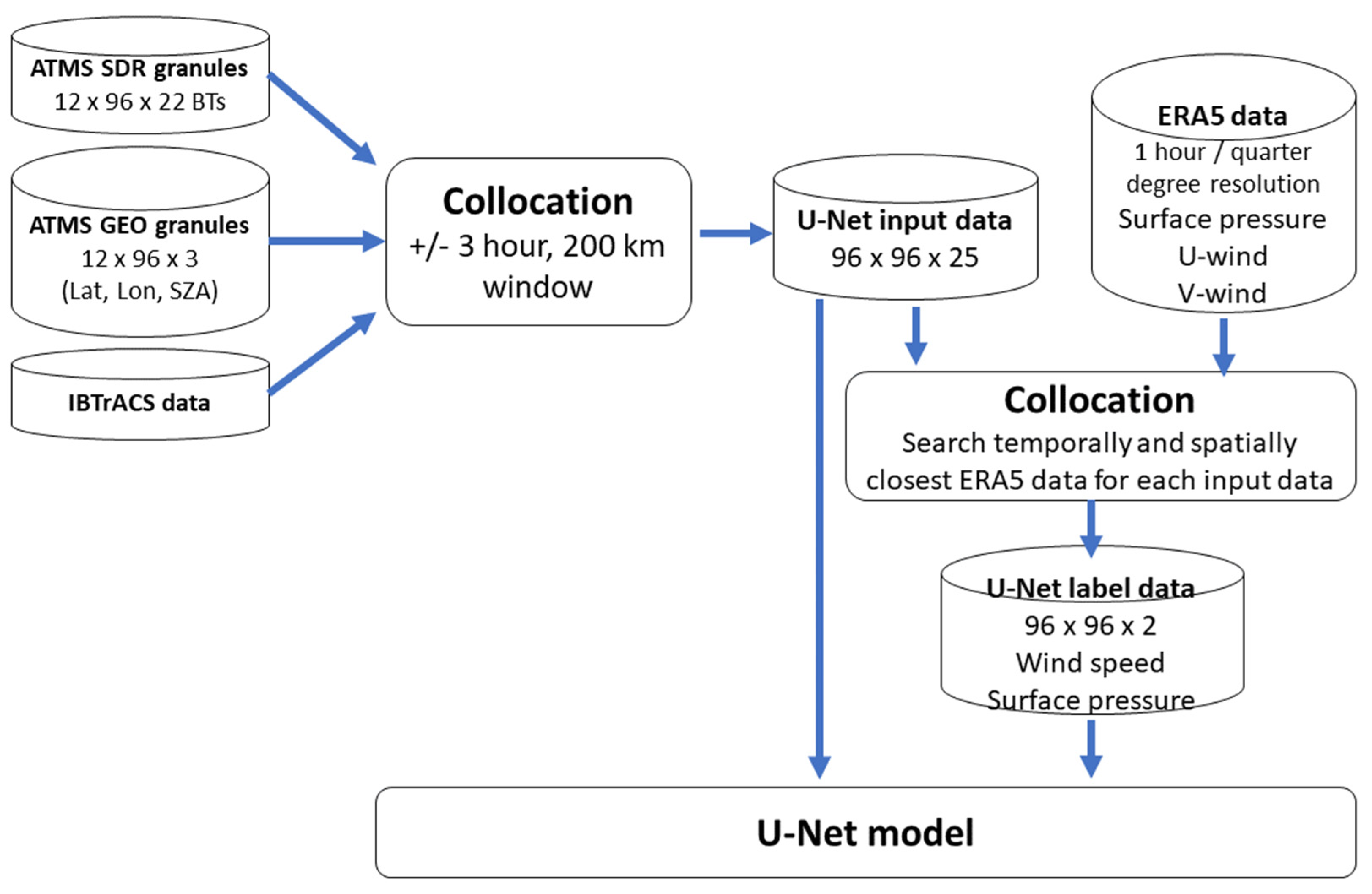
The collocation procedure to generate the U-Net model input is described as follows: First, relevant NOAA-20 ATMS input data granules were identified using the IBTrACS TC location data. NOAA-20 ATMS measurements, extracted from the ATMS SDR granules with 12 × 96 × 22 TBs and geolocation granules with 12 × 96 × 3 latitude, longitude, and satellite zenith angle, were searched for by using a reference +/− 3-h time window for each IBTrACS TC time and location, such that within each granule, at least one ATMS FOV would be found to have a distance less than 200 km from the IBTrACS TC latitude and longitude. Once the closest ATMS location is selected for each IBTrACS TC center, 47 scan lines observed after the location and 48 scan lines observed before the location are combined to generate 96 scan lines. As a result, a dimension size of 96 (FOVs) × 96 (scan lines) × 25 for each IBTrACS TC center, including 22 ATMS TBs and latitude, longitude, and SZA, was obtained.
Then, ERA5 data was collocated to the NOAA-20 ATMS observation locations. ERA5 data contains one-hour intervals and quarter-degree resolutions in latitude and longitude. For each NOAA-20 ATMS granule, the temporally and spatially closest ERA5 data (surface pressure, u-wind component (east-west), and v-wind component (north-south)) were identified. Once the closest ERA5 grid was identified for each ATMS FOV, the relevant variables were selected to match the associated ATMS field of view. Surface wind speed is the square root of the sum of the squares of the u-wind component and the v-wind component. As a result, the U-Net label data, 96 × 96 × 2 of surface pressure and wind speed, corresponding to input data, were generated. A detailed flowchart of this preprocessing is shown in
Figure 2.
Using the collocated ERA5 data and the ATMS reprocessed SDR data, 2230 samples were generated with each feature’s image dimensions of 96 × 96. To focus on pure ocean cases, each 96 × 96 sample whose pixels have only ocean surface type is selected, which leads to 266 samples. Within these samples, 191 samples originated from the North Atlantic Ocean, while the rest of the 75 samples came from the Western Pacific Ocean. The training data contains TC areas as well as non-TC areas. The sea surface wind speed in the training data varied between 0.01 m/s and 35 m/s, while the surface pressure varied between 958 hPa and 1036 hPa. As a result, about 30% of the samples were located in the Pacific basin, and 70% were in the Atlantic basin. ATMS input features included latitude, longitude, 22-channel brightness temperatures, and satellite zenith angle (SZA), with the usual labels’ references to surface pressure and surface wind speed at the hurricane center and the neighboring area from the collocated ERA5 dataset. With the 266 ocean surface-type samples, the train and test split function from the versatile Python scikit-learn open-source module (Version 1.3.2,
https://scikit-learn.org, accessed on 23 December 2023) was used to partition the dataset into two parts: 90% for training and 10% for testing, resulting in 239 training samples used for model training and 27 testing samples for model evaluation. Sci-kit Learn offers a broad array of tools for various machine learning tasks, including classification, regression, clustering, and dimensionality reduction. Additionally, 10% of the training data was used as validation data to validate and tune the model during the model training. The validation set offers essential insights into the model’s ability to generalize from the training data to “unseen” data, which facilitates the detection of overfitting caused by high variance and influences the fine-tuning of the model’s hyperparameters. Standardization was applied to all the input features. This normalization technique requires subtracting the data from the population mean and dividing the difference by the standard deviation, as described in Equation (4).
Here, X represents all pixel values across all sample images for a specific feature. μ and σ denote the mean and standard deviation calculated across all these pixel values in all samples, respectively. Consequently, this process yields z, the standardized vector, for a particular feature across all samples.
Robust normalization was performed on the label data. This has a similar expression to standardization but subtracts the data by the median and divides the difference by the interquartile range, as described in Equation (5).
Here, Y represents all pixel values across all sample images, corresponding to either the wind speed or surface pressure label. Ymedian is the median of these pixel values for each label. Q1 and Q3 denote the first and third quartiles of each label, respectively. Following the computation below, a normalized vector Ynew for a specific label across all samples is obtained.
To avoid possible outliers, robust normalization effectively minimizes the bias that the outliers create on the distribution of the data by not scaling the lower 25th percentile ( and the upper 75th percentile (. It is important to take note that the normalization procedure was performed differently between the features and labels. This prevents the use of improper normalization on certain features and improves the ability to single out a feature that may be detrimental to the training. For example, it would not be necessary to use robust normalization on the latitude and longitude because those are fixed constant values that will always fall within 90 degrees north to 90 degrees south and 180 degrees west to 180 degrees east.
The normalized and unnormalized training data are returned with 239 × 96 × 96 × 25 (inputs) and 239 × 96 × 96 × 2 (references) dimensions, respectively, along with the normalized and unnormalized testing data with the same dimensions except with 27 samples instead of 239. The normalized training dataset was fed into and trained with the U-Net model. The testing data was employed for the purpose of evaluating model performance. It is important to emphasize that the model’s prediction results were also normalized, mirroring the normalization applied to the input labels used for training, as outlined in Equation (3). Therefore, these normalized predicted results from the model required inverse normalization before proceeding with model evaluation.
Certainly, this research can also utilize other deep learning models, such as a traditional CNN or a deep neural network (DNN), which typically require thousands of data samples to train. It should be noted that training on both types of networks with the full dataset was also tested; however, the results were less accurate with more time-intensive training required, and so they are not reported here.
5. Discussion
There are limitations to using microwave sounder data to estimate surface wind speeds and surface pressures, in particular for tropical cyclones, which are associated with very high surface wind speeds and low surface pressures over oceans. Conical scan sensors such as AMSR-2 [
30] are better for estimating sea surface wind speeds because the sensor has low-frequency channels at 6, 7, and 10 GHz, as well as constant polarization. However, microwave sounders like ATMS have a wider (ATMS 2550 km vs. AMSR2 1450 km) swath and therefore have better global coverage. ATMS can measure vertical profiles of atmospheric temperature and water vapor so that we can estimate total atmospheric mass over the surface for estimating surface pressure. Thanks to AI technology applicable to three-dimensional atmospheres, U-Net can utilize horizontal features to mitigate the limitations of ATMS surface signals affected by precipitation. Liu et al. (2023) [
31] apply U-Net to improve retrieved precipitation rates. Using multiple ATMS channels, the limb effect can be taken into account. Zhang et al. (2017) [
25] demonstrated how the ATMS limb effect can be corrected by using all ATMS channels. Another limitation is that passive microwave signals are often saturated for very high surface wind speeds. Active sensors such as Radarsat-2 and Sentinel C-band missions have a very weak incidence and azimuth angle dependency with no indication of saturation for the strongest sea surface wind speeds [
32,
33].
Intuitively, surface pressure and surface wind speed of the TC eyewall region can be retrieved with a single latitude and longitudinal point for every ATMS measurement sample, which has been demonstrated by previous studies [
10,
11,
12,
13,
14,
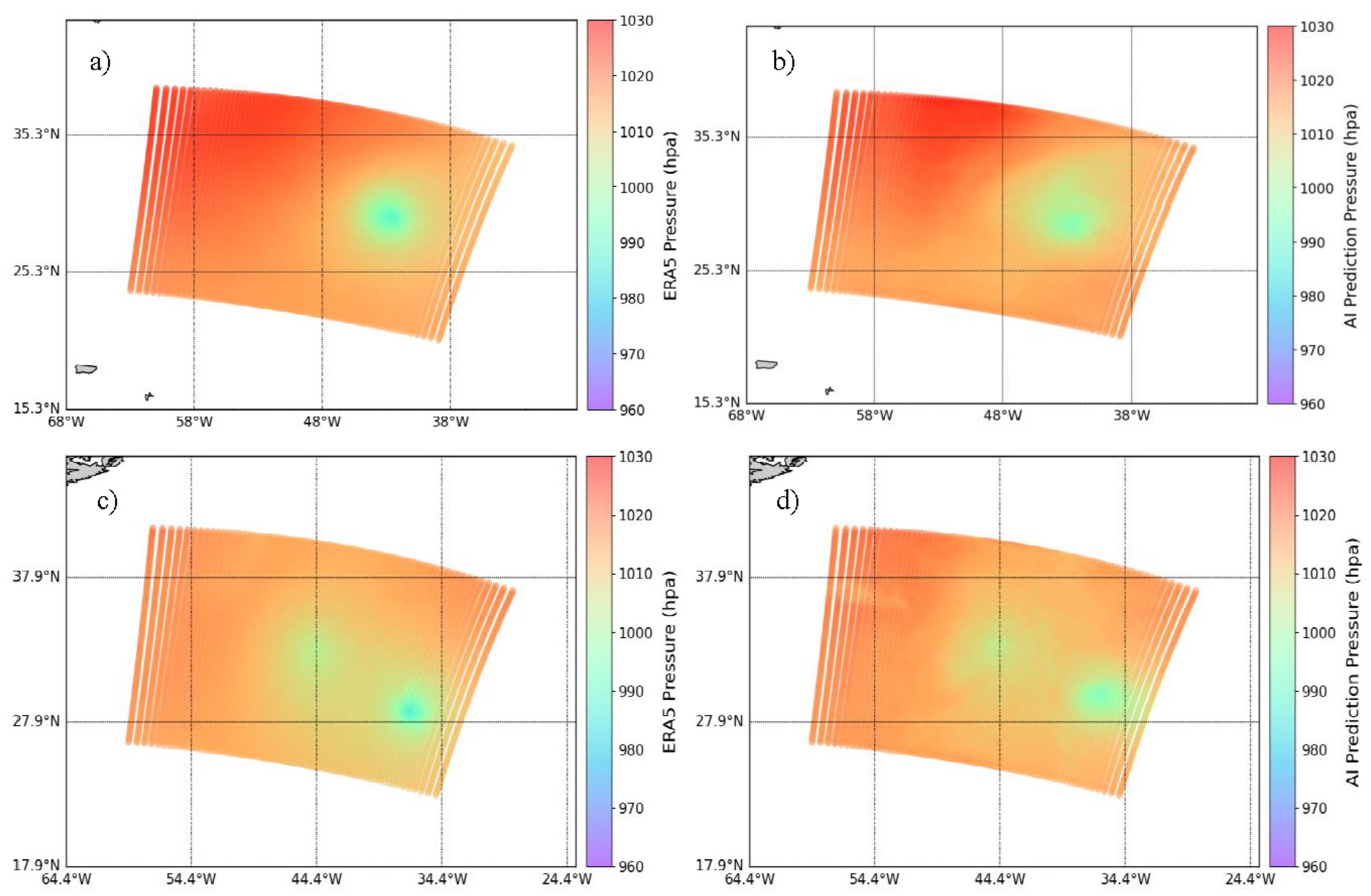
15]. However, this is not an ideal situation because the atmosphere and surface states surrounding TCs are also crucial factors affecting rapid changes near TC areas. Hence, using a multi-dimensional image space would be more suitable for predicting the surface wind speed and surface pressure images surrounding each TC and extracting the maximum wind speed and minimum surface pressure from those images as the estimate of TC intensities as seen in the results.
The U-Net algorithm employed in this study showed multiple advantages for the retrieval of surface wind speed and surface pressure images surrounding the TC eyewall region using multi-dimensional input images. Firstly, the U-Net algorithm only requires a few images to train and can reach a relatively accurate result [
19], which exactly meets this study—only 266 pure ocean images are available. Secondly, the model is quite efficient. The train time was no more than two hours on a server with three CPUs (Intel Xeon CPU E5-2680 2.5 GHz each) and 64 G memory requests, and without GPU support. Also, the main feature of the U-Net algorithm—learning image segmentation in an end-to-end setting—is well extended in this study, which is used to learn the images of ATMS measurements and geolocation information to predict relative surface wind speed and surface pressure images.
Certainly, the results shown in
Section 4 indicate that the accuracy of surface wind speed for the TC eyewall region could still be improved. One considerable improvement is to refine the input features. Some ATMS channel measurements may not provide information on TC intensity, such as channels with weighting functions peaking in the upper atmosphere, which are not sensitive to near-surface variations like TC. Removing these channels from the input data may avoid additional interference and improve the prediction accuracy. Although the microwave channels are not sensitive to the cloud, for the TC eyewall area with heavy cloud surrounding, the cloud information may also be a considerable factor in affecting the estimation accuracy of TC intensity. In terms of training sample size, the 239 TC data samples could be inadequate to reach the highest prediction accuracy for the U-Net used in this study. It is a good idea to further collect input data to retrain the model. Finally, outliers may still exist in the ERA5 and IBTrACS data, particularly for cases of high wind speed, which affects the model’s accuracy and evaluation when outliers are passed to the model and employed as references. Quality control for ERA5 and IBTrACS data before data collocation would be worthwhile for this work. In addition, the model architecture and related hyperparameters may also be fine-tuned and optimized. However, the preliminary model and data used in this study have demonstrated similar prediction accuracy when compared with traditional methods, indicating that the U-Net model is likely to achieve higher accuracy for TC intensity estimation after the above factors are considered and improved.
6. Summary and Conclusions
A modified U-Net algorithm was employed to estimate tropical cyclone intensity, as represented by surface wind speed and surface pressure surrounding the TC areas. ATMS data and collocated ERA5 were chosen based on the time and location of TCs in the IBTrACS database. A total of 266 pure-ocean image sets were selected from the period 2018 to 2021, located in the Northwest Pacific and North Atlantic basins, to train and test the U-Net model. Each set includes 25 input image features (22 ATMS TBs, longitude, latitude, and SZA) and 2 label images (surface wind speed and surface pressure).
The U-Net, which originally used a binary-entropy loss function, was updated to instead utilize a mean square error (MSE) metric to match a regression problem in this study, and the activation function was changed from SoftMax to linear in the last layer. The input image size was designed to be 96 by 96 for efficient processing, which aggregated eight contiguous ATMS granules surrounding the TC areas to further incorporate possible spatial relationships in the areas surrounding the TC during model training and testing.
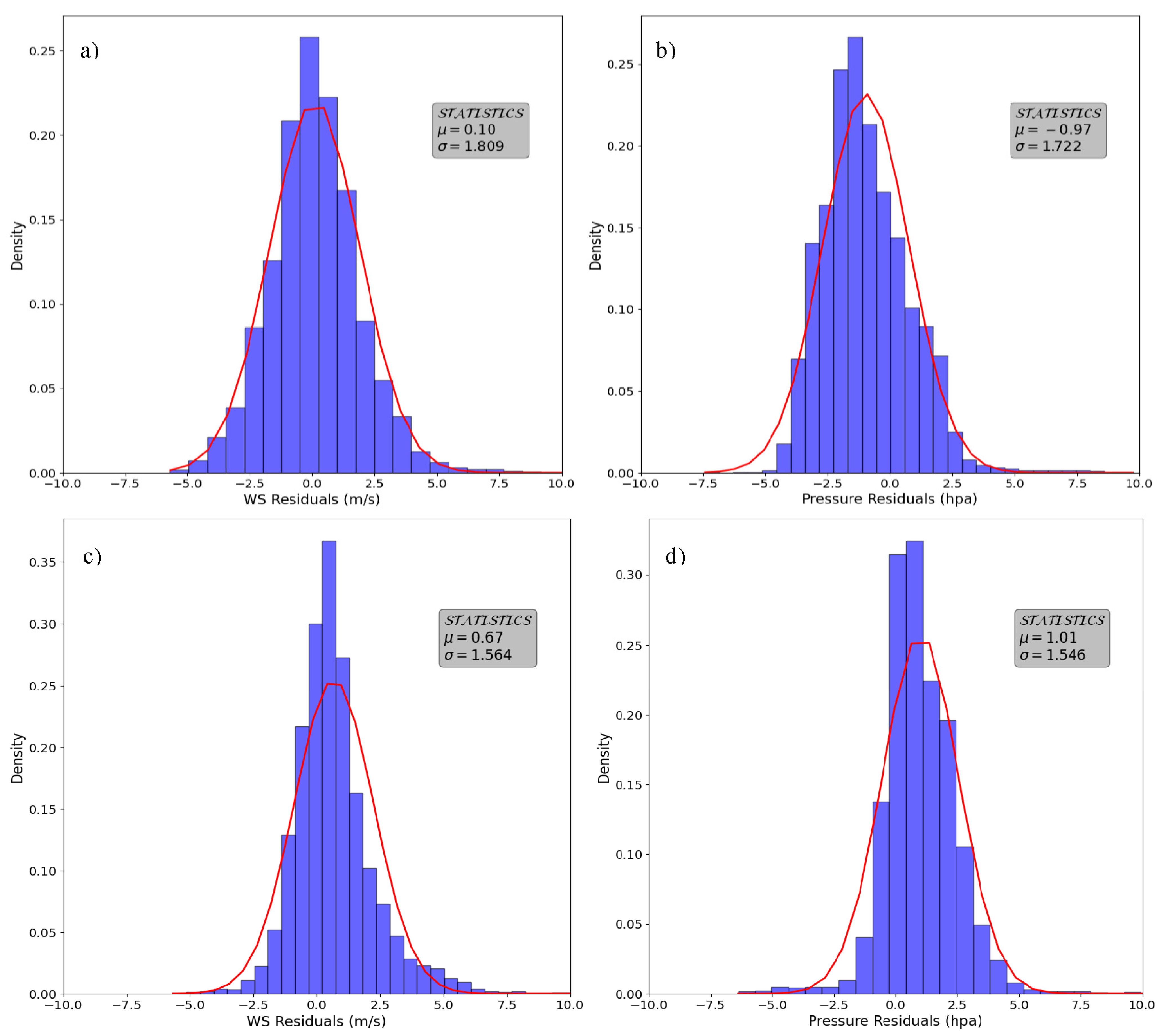
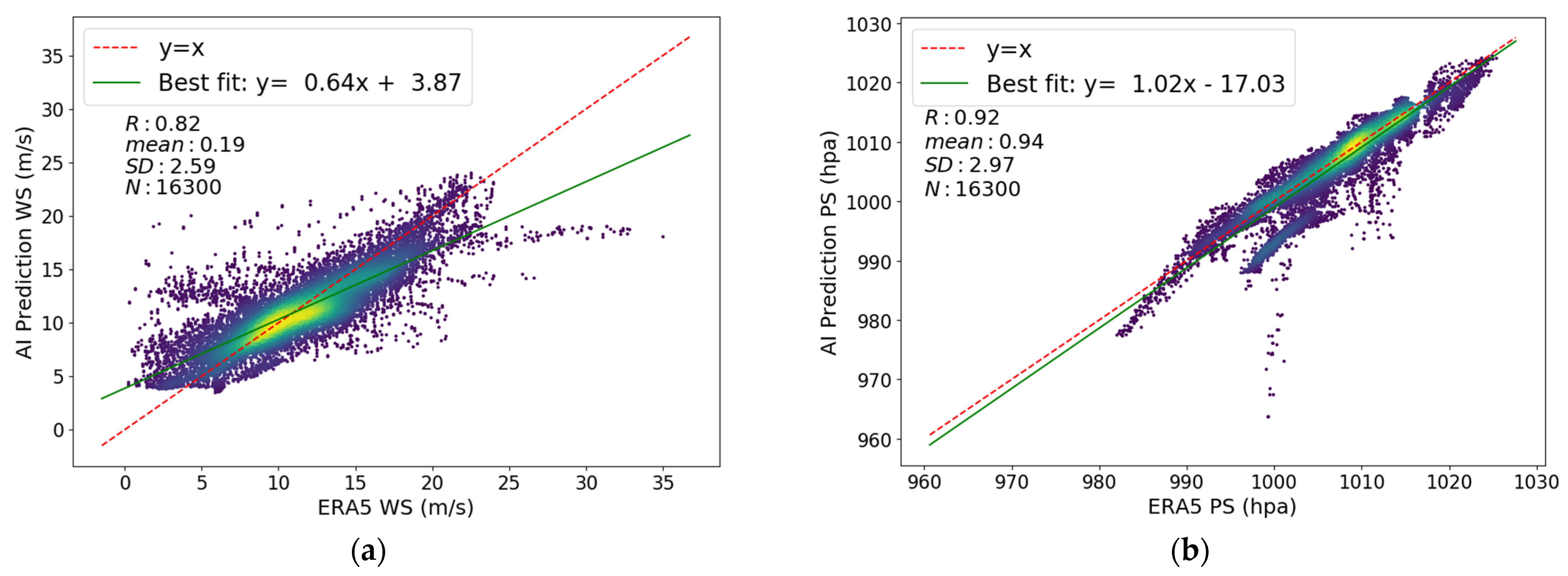
The U-Net prediction showed promising results. The residual biases and standard deviations between the U-Net predicted and ERA5 reference labels were about 0.15 m/s and 1.95 m/s for wind speed and 0.48 hPa and 2.67 hPa for surface pressure, respectively, after cloud screening for each ATMS pixel. This indicates that the U-Net model is effective for near-TC wind speed and pressure estimates for more general over-ocean conditions. The strength estimation (surface wind speed and surface pressure) of tropical cyclones using ATMS measurements in this study revealed promising results compared to the previous study [
15], which used the conical microwave instrument, AMSR-2. There may still exist opportunities to improve accuracy, particularly for high surface wind speeds in the TC eyewall region, as discussed in
Section 5. Refining the input features, adding more data samples, and considering quality control for ERA5 and IBTrACS data are expected to improve the model’s accuracy.
Future work, in addition to those aspects mentioned above, would involve fine-tuning the model, particularly exploring the possibility of more epochs, carefully selecting the learning rate base and decay, adding regularization, and other overfitting methods that could have affected the prediction results. More rigorous sensitivity tests to determine the optimum selection of input channels could also be conducted. This could lead to visualizations where the eye region and its associated eyewall structure are better predicted.


