1. Introduction
Monitoring the isotopic content of water vapor provides valuable information about the water cycle, including cloud feedback and radiation budgets, etc. [
1,
2]. Heavier water isotopologue HDO condenses more actively and evaporates less actively than the main isotopologue H
216O, due to differences in the saturation vapor pressure of these two molecules. There are two stable isotopes of hydrogen, H with a relative abundance of 99.984%, and D with a relative abundance of 0.015%, and three stable isotopes of oxygen,
16O,
17O, and
18O, with relative abundances of 99.759%, 0.037%, and 0.204%, respectively [
3]. Since the numerical values of isotope abundance ratios in nature are very small, it is more convenient to describe the isotopic composition of a given water sample as the deviation of the abundance ratio from a standard value, expressed in per mil (‰). We have thus defined the delta notation defined as:
Here, HDO/H
2O is the ratio of HDO and H
2O abundance for a given water sample, and HDO/H
2O
VSMOW (=311.53 × 10
−6) is the HDO/H
2O of Vienna standard mean ocean water (VSMOW) [
4].
The stable isotopes of HDO in the atmosphere are affected by various factors, such as latitude, altitude and distance from the coast, etc. [
1,
2]. For example, the international standards used for the determination of
18O and D isotope abundance ratios of VSMOW and Standard Light Antarctic Precipitation (SLAP) are 155.76 ×10
−6 and 89.1 × 10
−6, respectively. However, the δD of SLAP is −428‰ when referring to VSMOW [
5]. The difference results in the depletion of HDO and indicates global and regional climate change [
6,
7]. Therefore, studying the isotopic composition of water vapor in the atmosphere is very helpful in identifying the sources and sinks of water cycling and climate change. Moreover, the variation in abundance is also related to ocean pollution, which helps in identifying the sources of pollution.
Due to its importance, in situ, ground-based and satellite remote sensing methods based on absorption spectroscopy methods have been developed for the measurement of water vapor isotopes. The in situ methods include Cavity Ring-Down Spectroscopy (CRDS), which is a kind of high sensitivity (precision is 5.65 ppm for H
2O) technology for greenhouse gases detection [
8,
9]; this technology for HDO detection has recently been discussed by Michel et al. [
10] and Chang et al. [
11]. Michel used a quantum cascade laser to measure H
216O and H
218O spectra in 7.2 μm, and the detection limit for δ
18O was 0.42‰. Chang used a 2.65 μm tunable diode laser to measure H
216O, H
218O and HDO spectra in different samples. The traditional instrument of ground-based methods is the Fourier Transform Infrared Radiometer (FTIR), such as the Total Carbon Column Observing Network (TCCON) and the Network for the Detection of Atmospheric Composition Change (NDACC). The data are usually used for the calibration of satellite observations [
7,
12]. The SCIAMACHY instrument on board the satellite ENVISAT was the first instrument to provide global retrievals of water isotopes with high sensitivity near the ground. However, due to degradation, the data record of SCIAMACHY HDO only covers the years 2003 through 2005, and unfortunately, the connection to the entire ENVISAT was lost in April 2012. Other studies on the global HDO distribution research based on GOSAT, AIRS and TROPOMI satellites were investigated, respectively, by Christian Frankenberg, Robert Herman and Andreas Schneider et al., and the results of these studies were compared and analyzed with data from TCCON [
13,
14,
15,
16,
17,
18,
19]. Furthermore, the researchers have also paid much attention to the observation of Martian HDO abundance in recent years, because it provides unique insights into the evolution and climatology of its atmosphere [
20,
21]. The above studies show that the multiple methods of observation can provide more reliable results for determining the abundance of water vapor isotopes.
The analysis of monthly mean precipitation in Northwest China (NW) (35–50°N, 74–105°E) indicates that the arid and semiarid regions of NW experienced a significant wetting trend in summer during 1961–2010. Undoubtedly, this trend had substantial effects on the ecological environment and social development, as well as the lives of people. In addition to the increased evaporation, the change in atmospheric circulation is another important factor [
22]. The TP is known as ‘the third polar’ in geography, and its atmospheric exchange will influence East Asia and even the world’s climate. For this purpose, we are attempting to develop a new method for the water vapor isotopic abundance measurement and provide the fundamental data for the climatic research of NW and the TP. Therefore, it is significant to develop a portable device and carry out water vapor isotopic abundance measurements in order to enhance our understanding of climate change and atmospheric circulation.
In recent years, the laser heterodyne radiometer (LHR) has been greatly improved with high-quality performance in monitoring atmospheric trace gases at a small size and low cost, attracting lots of attention from related researchers. LHRs have been successfully used to measure atmospheric O
3, CO
2 and CH
4, etc., from the ground using either a quantum cascade laser (QCL) or distributed feedback (DFB) laser as a local oscillator (LO) [
23,
24,
25,
26]. Several laser heterodyne radiometers in the 3~5 μm band were realized in our laboratory, and solar spectra through the entire atmosphere were obtained [
27,
28,
29]. Accounting for the aforementioned reasons and fundamentals, we have developed an LHR operating at 3.66 μm for monitoring atmospheric water vapor and its isotopic abundance.
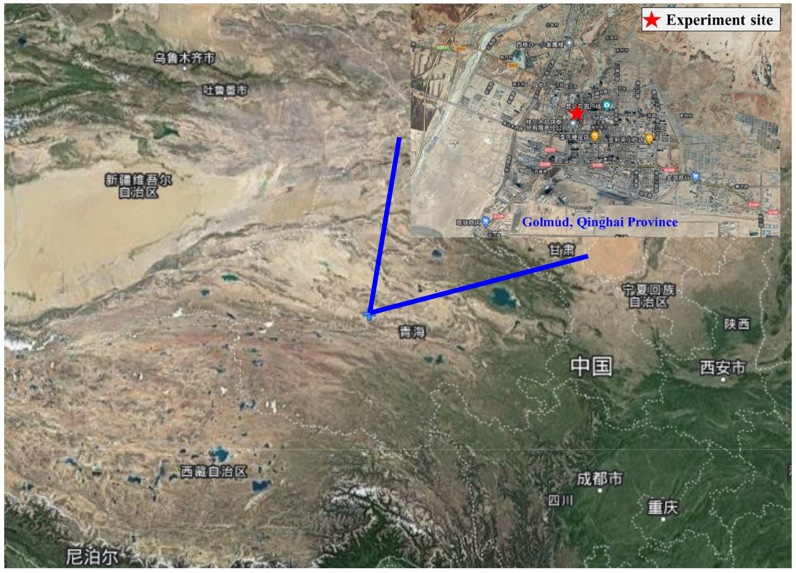
In order to improve the data quality of the H2O and its isotopic absorption spectrum, the combined ratio of laser to solar beam is optimized from 50%: 50% to 10%: 90%. The scanning time, the integral time and the filter band are optimized in this work for obtaining a high resolution and high signal-to-noise ratio. The spectral resolution is 0.0098 cm−1, theoretically. Additionally, the inversion method of water vapor isotope abundance was studied to realize the simultaneous inversion of H2O and HDO column densities. The experimental campaign operated in Golmud (94.9° E, 36.4° N, Qinghai Province; the altitude is 2810 m) in August 2019. The synthetic spectra of HDO and H2O were obtained simultaneously, and the HDO abundance was retrieved and analyzed.
2. Materials and Methods
2.1. Instrument Design and Operation
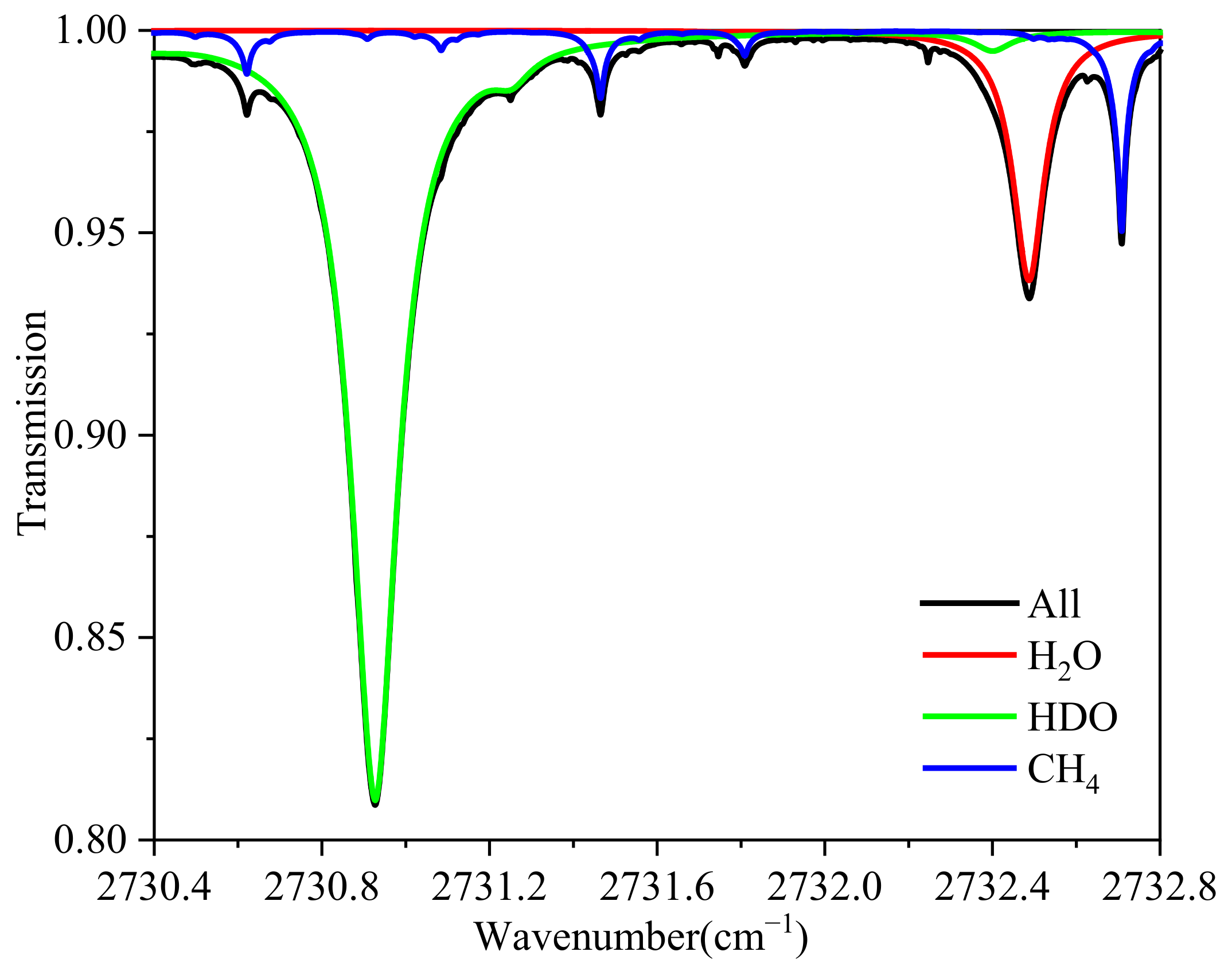
The simulation of the total atmospheric HDO and H
2O absorption spectrum by the Line-By-Line Radiative Transfer Model (LBLRM) at 3.66 μm based on the standard atmospheric model (1976) is shown in
Figure 1. The absorption intensity of HDO (υ = 2730.9274 cm
−1, S = 2.777 × 10
−24 cm
−1/(molec·cm
−2)) and H
2O (υ = 2732.4932 cm
−1, S = 1.206 × 10
−24 cm
−1/(molec·cm
−2)) is an optimal wavelength region in the mid-infrared. The absorption spectra of HDO and H
2O are within 3 cm
−1, and the wavelength range can be covered in a single scanning by a diode laser. There is almost no interference absorption of other molecules in addition to CH
4. The laser heterodyne radiometer is an ideal instrument for this purpose, and the method can obtain an accurate of the HDO/H
2O ratio measurements.
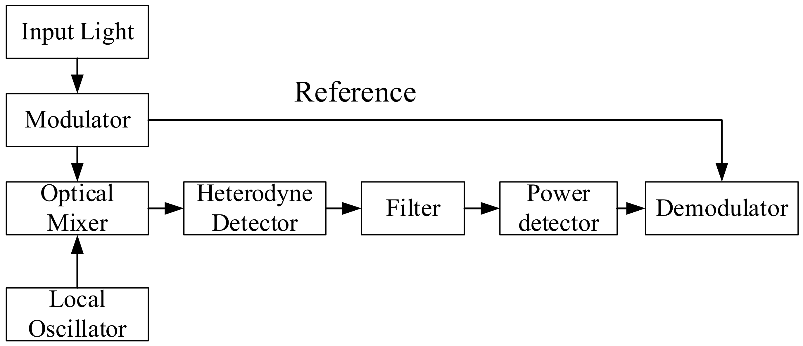
Laser heterodyne spectroscopy technology adopts a narrow linewidth laser to mix with the input signal light. The theoretical value of the total photocurrent generated by the detector is:
where
ALO and
AS are the amplitude of
LO and signal light,
υLO and
υS are the frequency of
LO and signal light,
η is the efficiency of the detector. The second item is the heterodyne signal and its power is:
where
PLO and
PS are the power of
LO and signal light. The power of the heterodyne signal is proportional to the
LO power and the signal light power. When the signal light power is weak, the light intensity information it carries can be amplified by the local oscillator light, the method can reduce the difficulties of spectral detection compared with direct detection. Then, the generated heterodyne signal is filtered, detected and demodulated to obtain the absorption spectrum signal of the atmospheric gases. The signal processing flow is shown in
Figure 2.
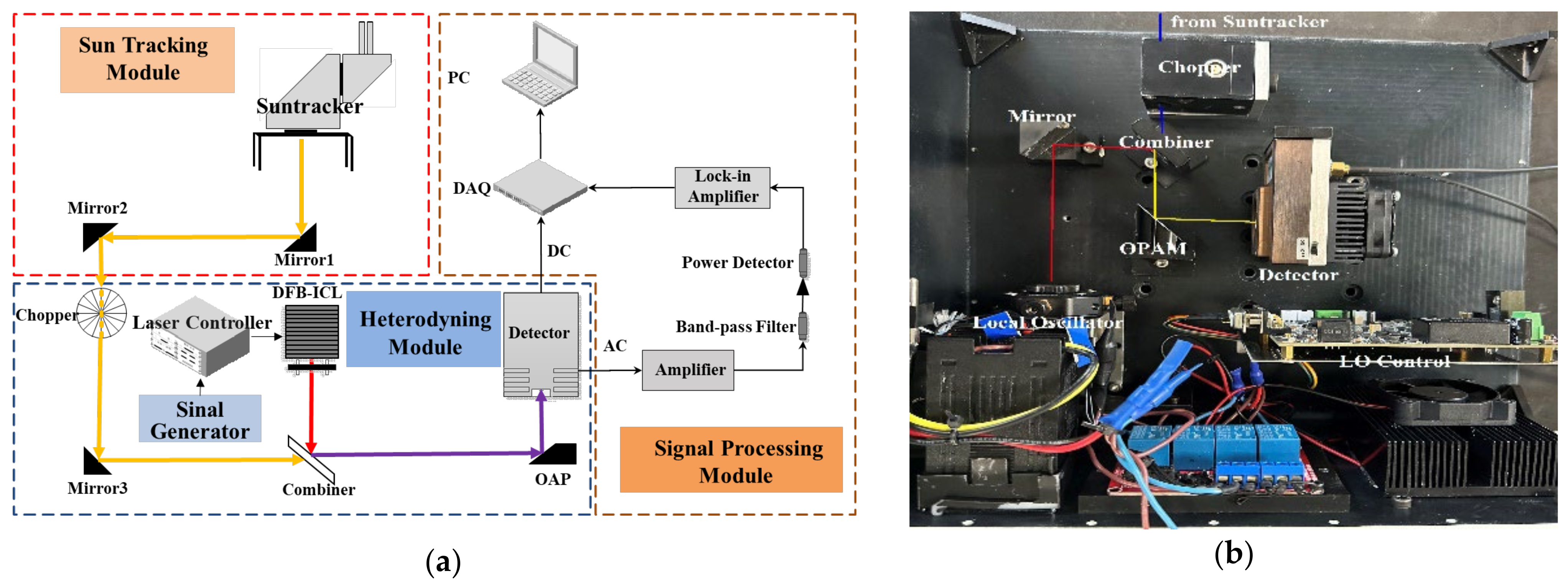
As shown in
Figure 3a, the self-designed LHR consists of three modules: namely, the sun-tracking module, the heterodyning, and the signal-processing module [
27,
28,
29]. The self-designed LHR utilizes a DFB interband cascade laser (ICL) as an LO, operating at 3.66 μm with a power output of several milliwatts (Nanosystems and Technologies, Meiningen, Germany). The DFB-ICL exhibits excellent performance in terms of narrow line width and continuous wavelength change in scanning mode, ensuring a high spectral resolution signal. The incoming sunlight is captured by a solar tracker and mixed with the LO. To promote the heterodyne signal, the combined ratio of the LO and sunlight is about 10%: 90%. The mixed light is focused by the off-axis parabolic (OAP) mirror and input into the detector. The focal length of the parabolic mirror is 2 inches, and the focus is located on the photosensitive surface of the detector. The PV-4TE-4 (VIGO Photonics, Warsaw, Poland) detector’s sensitivity is up to 1.0 × 10
11 cm∙
/W, and its small active area (0.1 mm × 0.1 mm) and its temperature are controlled at 195 K, which can reduce the noise of the medium signal. The compact heterodyning module is shown in
Figure 3b. Then the medium signal is processed by a radio frequency (RF) device and demodulated by a lock-in amplifier (LIA, OE1201, Sine Scientific Instruments, Guangzhou, China). A voltage noise as low as 9 nV/
meets the demands of spectral measurements. In summary, the spectrum of the input signal can be obtained with high sensitivity by the LHR.
The HDO abundance based on the LHR is reported for the first time; the parameters of the LHR were comprehensively considered to obtain accurate absorption spectra of H
2O and HDO, such as scanning period, integral time and filter band. According to the signal-to-noise ratio (SNR) and instrumental line shape (ILS) of the LHR, the SNR is proportional to the integral time(
τ) and filter band(
B), while the spectral resolution is inversely proportional to them [
30].
In addition, fc is the frequency of the low-pass filter, which is related to the integration time; fLO(ω) is the line shape function of the LO; HB(ω) is the function of the bandpass filter in the frequency domain; hfc(ω) is the function of the low-pass filter.
The passband of the radio filter is 10~50 MHz (single bandwidth is 40 MHz, dual bandwidth is 80 MHz). The detailed parameters of the LHR are shown in
Table 1.
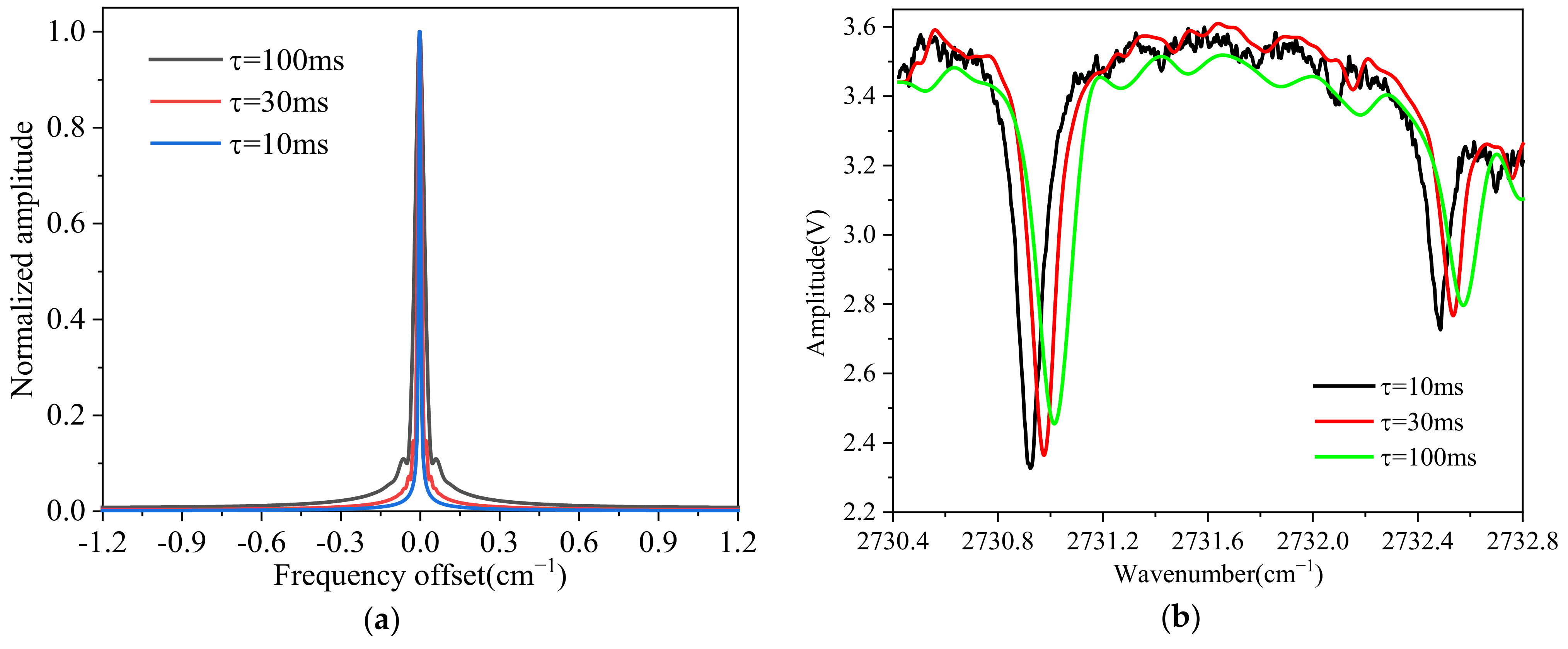
The simulated ILS of the LHR and the measured spectra with different integration times are shown in
Figure 4. There are three suitable choices for the integral time of LIA, namely, 10 ms, 30 ms and 100 ms, and the corresponding spectral resolutions are 0.0098 cm
−1, 0.0194 cm
−1 and 0.043 cm
−1, respectively. The spectral bandwidth of H
2O and its isotope at 10 km is about 0.018 cm
−1. The integral time changed from 10 ms to 100 ms and the SNR increased, while the spectral resolution decreased. Additionally, the larger the integral time, the more obvious the delay effect. Therefore, the integral time was set to 10 ms in this study to achieve a more precise measurement of tropospheric water vapor and its isotopic spectrum.
Taking the change rates of water vapor density and solar angle into consideration, the acquisition period should be completed in several minutes. We chose a scanning period of 15 s with a 20% duty ratio, and the signal was averaged 12 times to improve the SNR. The total acquisition cycle costs 3 min in this case.
2.2. Experiment Site
Golmud is located at the outskirts of the Qaidam Basin and in the interior of the Tibetan Plateau (TP) (
Figure 5). Because the annual average rainfall is only about 41.5 mm, while evaporation exceeds 3000 mm, Golmud is classified as having a continental plateau climate. Golmud is a typical city in NW and the TP; the research on atmospheric composition and exchange in this area helps to enhance our understanding of the climate of the TP and NW.
2.3. Retrieval Method
The measured heterodyne spectra were retrieved by the Optimal Estimation Method (OEM), the method was developed by C. Rodgers [
31] and is widely used in atmospheric retrieval and obtains credible results with self-setting parameters, such as atmospheric layers, iterations and iteration type.
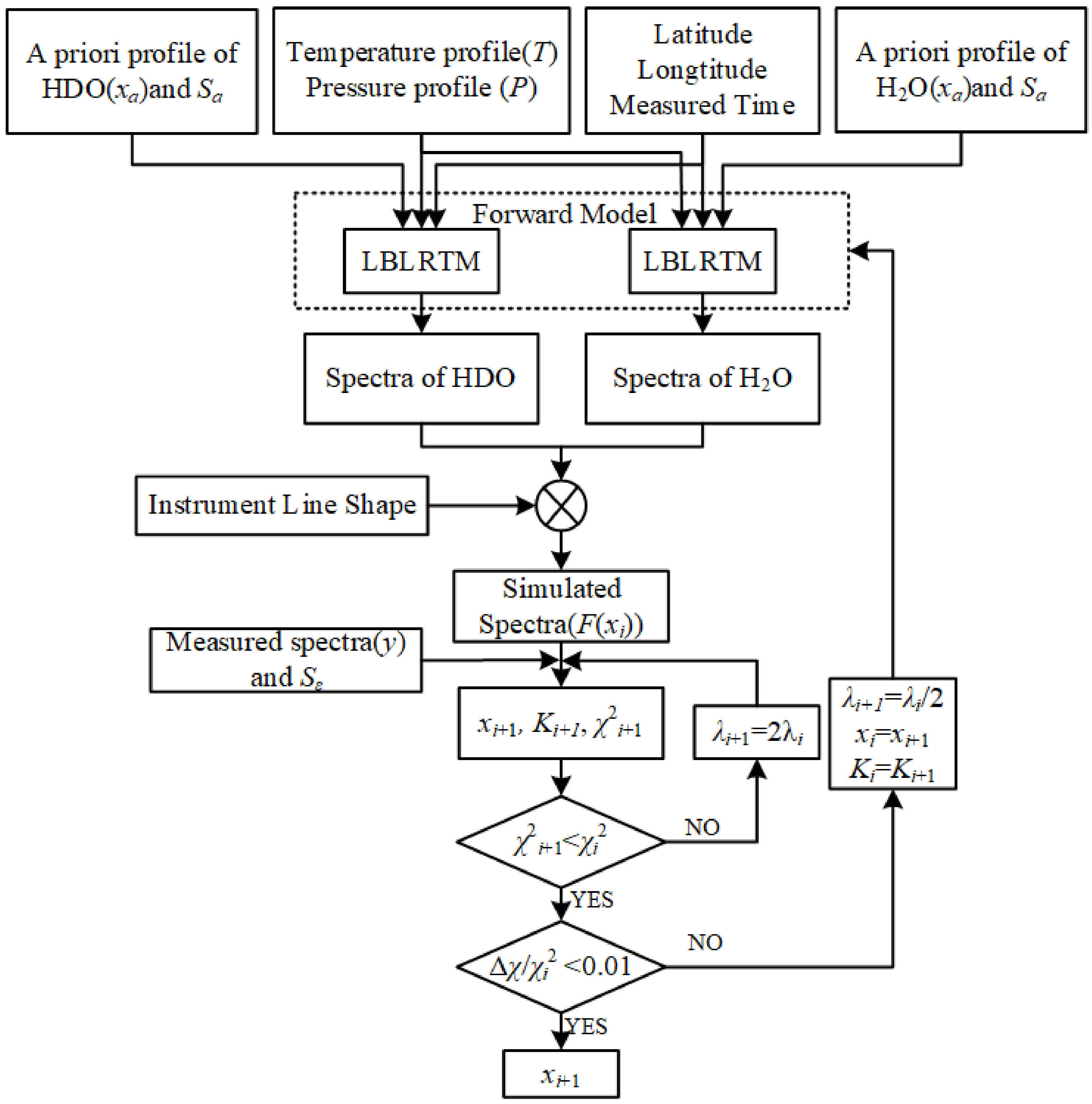
The progress of HDO/H
2O inversion is shown in
Figure 6. In this research, the LBLRTM (version 12.9), which is an accurate software for the research on atmospheric transmittance, radiative transfer and cooling rate [
32], was used in the forward model for HDO and H
2O density retrieval.
During the inversion in this research, HDO and H2O were treated as independent species without any side constraints (besides the similarity in the prior profile) imposed on the HDO–H2O functional relationship on the a priori covariance matrix. The density of HDO and H2O output individually. Another parameter, such as the continuum baseline fitted with a second-order polynomial, could reduce the influence of the LO scanning during the inversion.
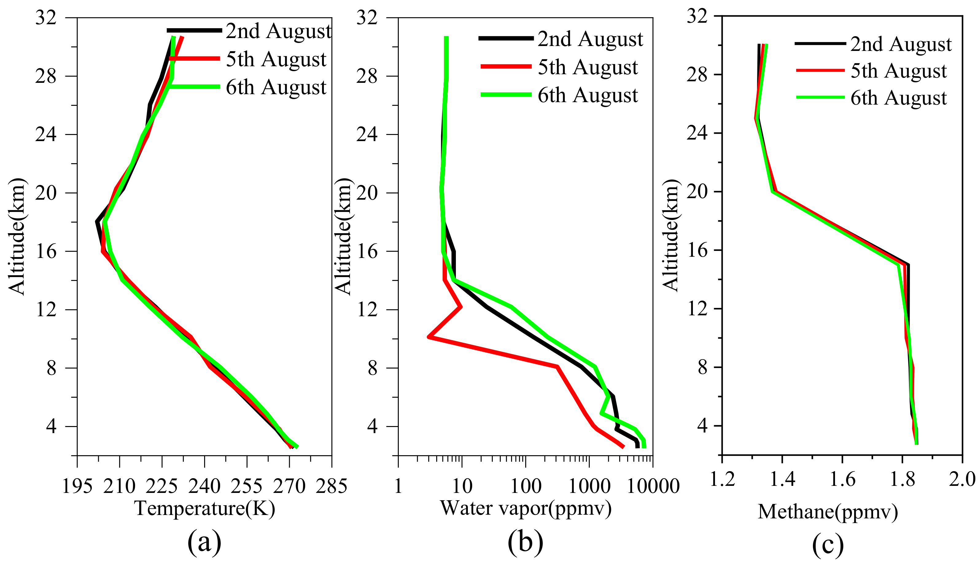
Additionally, the atmospheric model profiles of interfering species with weak absorption (mainly CH
4) were adopted to reduce the difference. The temperature, a priori water vapor and methane profiles were obtained from the European Center for Medium-Range Weather Forecasts (ECMWF), as shown in
Figure 7. The concentration of CH
4 was about 1.84 ppmv and almost unchanged below 15 km, while the concentration of water vapor changed greatly in three days and decreased exponentially with height; almost 90% of HDO and H
2O was concentrated below 6 km altitude.
In the retrieval algorithm, the forward model
F is defined by:
The vector
y is the measured spectra with error
ε,
x is the state vector of atmospheric profiles. The OEM is a Levenberg–Marquardt (LM) iterative algorithm based on the nonlinear-least-square method and minimizes the cost function to:
where
Sε and
Sa are the measurement covariance matrix and a priori covariance matrix.
xa is the a priori vector. For the faster speed of iteration of the state vector, the Gauss–Newton iteration is used in the inversion:
where
K is the Jacobian matrix, and it is the important parameter that affects the retrieval results;
λ is the Lagrange factor, and
λ is chosen at each step to minimize the cost function; and the subscript represents the number of iterations [
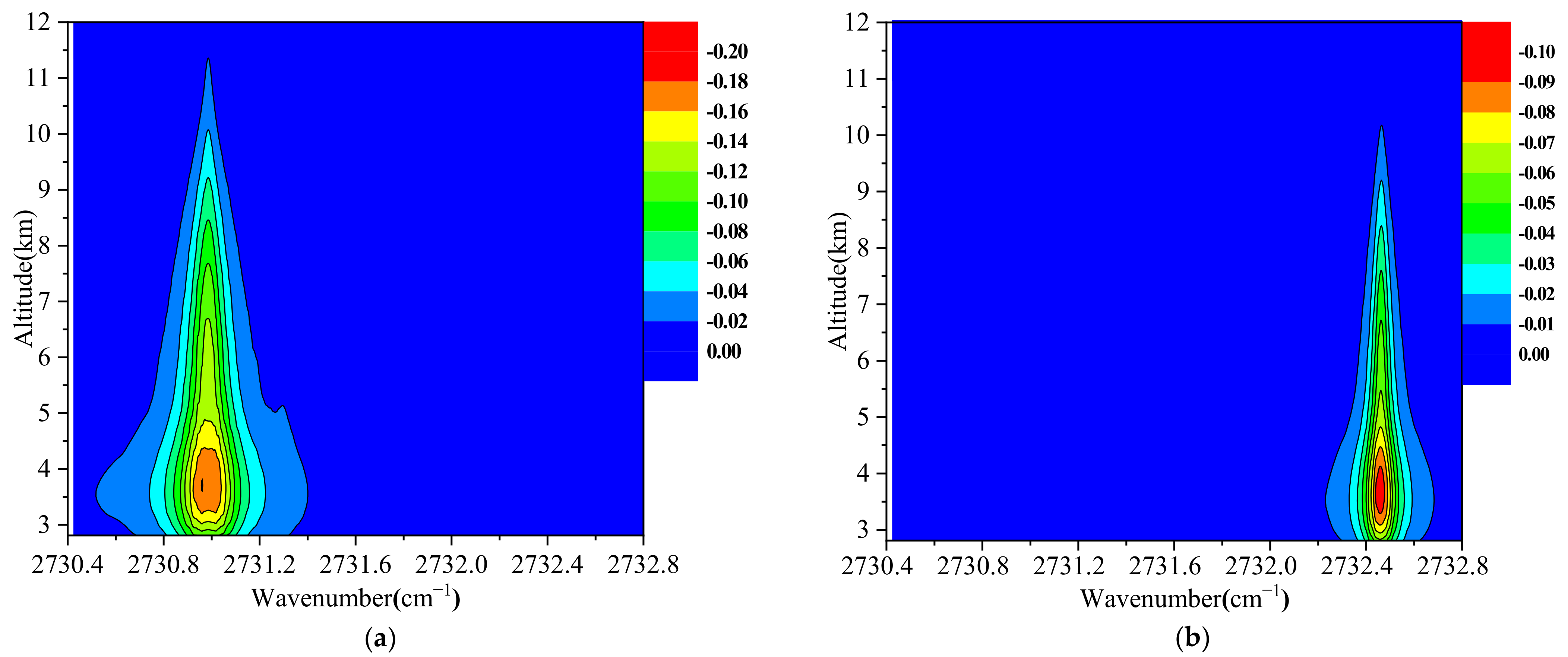
31]. The Jacobian matrix is calculated by:
Each element is the partial derivative of a forward model element with respect to a state vector element, i.e.,
Kij =
∂Fi(
x)/
∂xj. The Jacobian value is the kernel parameter in the retrieval process, and it should be changed in each iteration, with an absolute value proportional to the intensity of absorption [
31]. The Jacobian values of HDO and H
2O are shown in
Figure 8.
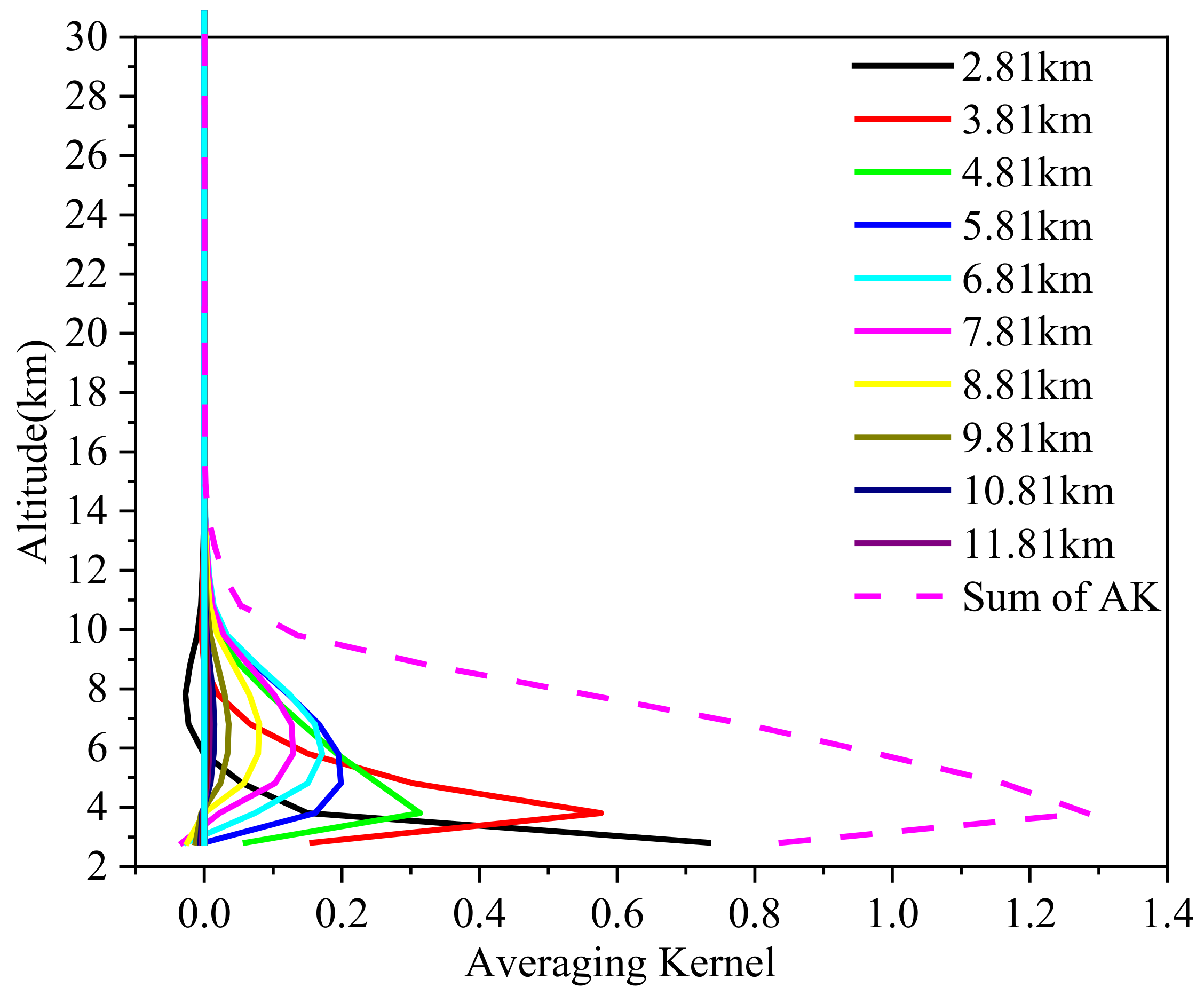
Because of the big variation in water vapor density, the appropriate altitude grid is helpful for more precise retrieval results. The averaging kernel (AK) provides a simple characterization of the relationship between the retrieval and the actual state. The width of the AK gives the vertical resolution of the instrument at the corresponding altitude, and the sum of the AK values is proportional to the information retrieved from the measurement rather than a priori [
25]. The formula of the AK is described by:
The averaging kernels of H
2O with 1 km spacing were calculated to optimize the altitude grid, and the results from the ground (2.81 km) to 30 km are shown in
Figure 9.
Analysis of the averaging kernels shows that the half-width near the surface was 1~2 km, while the width the above 4.81 km was much broader than the simulated 1 km resolution of the input altitude grid, indicating that much of the retrieved information was redundant.
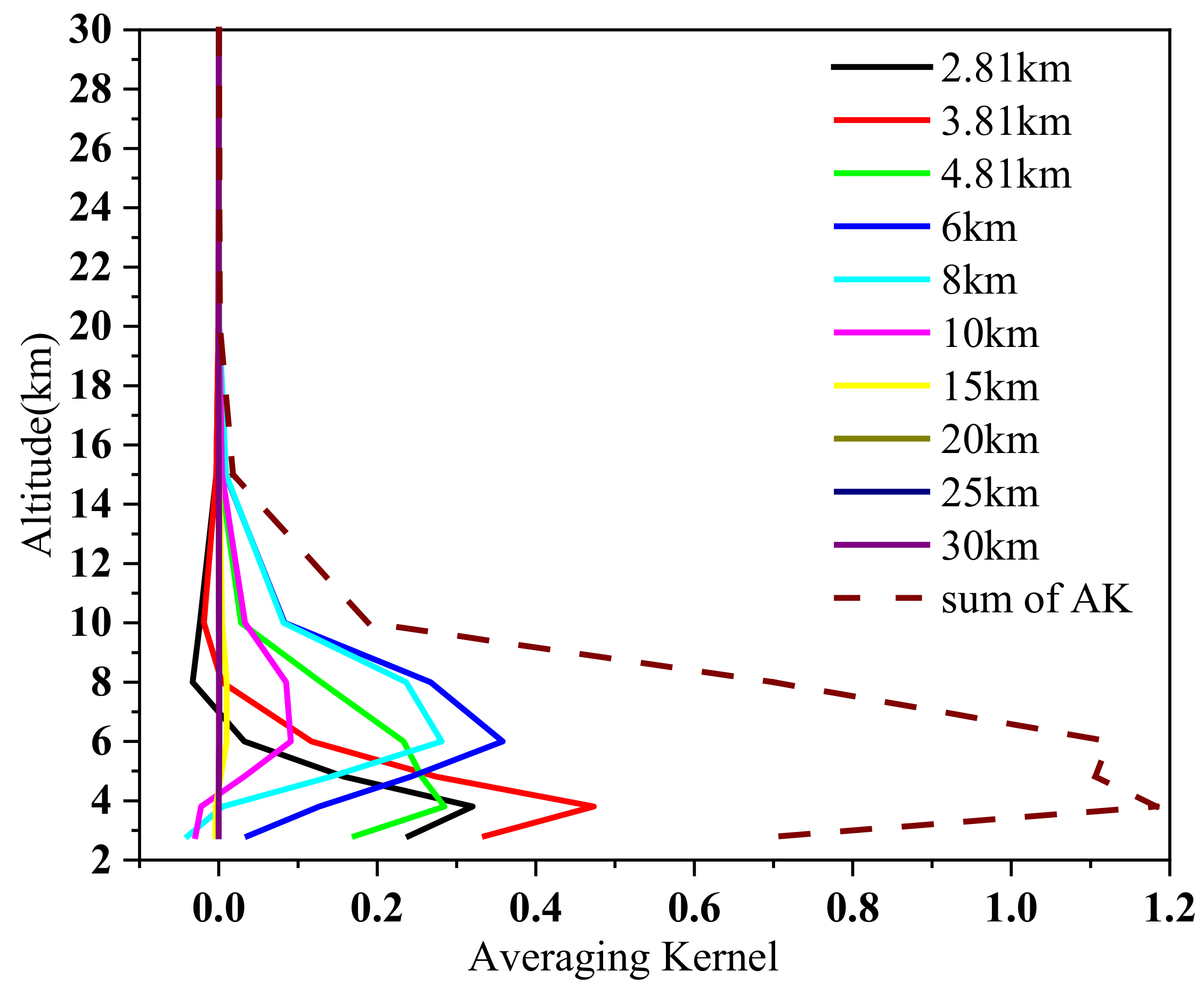
Therefore, the retrieval layers were divided into 10 layers from the surface to 30 km. The height resolutions were 1 km (surface to 6 km), 2 km (6 km to 10 km) and 5 km (10 km to 30 km) respectively, accounting for the characteristics of atmospheric water vertical distribution. The averaging kernels were recalculated (
Figure 10) after the refined altitude grid, the results indicate the altitude was almost associated with each AK peak, and the widths of AK below 8 km were more consistent with the altitude grid. The proper height spacing not only reduces the redundant information but also speeds up the calculation during the inversion.
Similar to the retrievals of other greenhouse gases in the mid-infrared, the sensitivity of inversion is much lower above 10 km; thus, the retrieval of profiles is not easily feasible, because the Jacobian and averaging kernel values of HDO and H2O are higher under 10 km than above 10 km. The densities of HDO and H2O can be retrieved from measured spectra, but it is extremely difficult for the retrieval process above 10 km. Hence, we focused on the retrieved total column amounts, which are more robust estimates in the mid-infrared.
3. Results
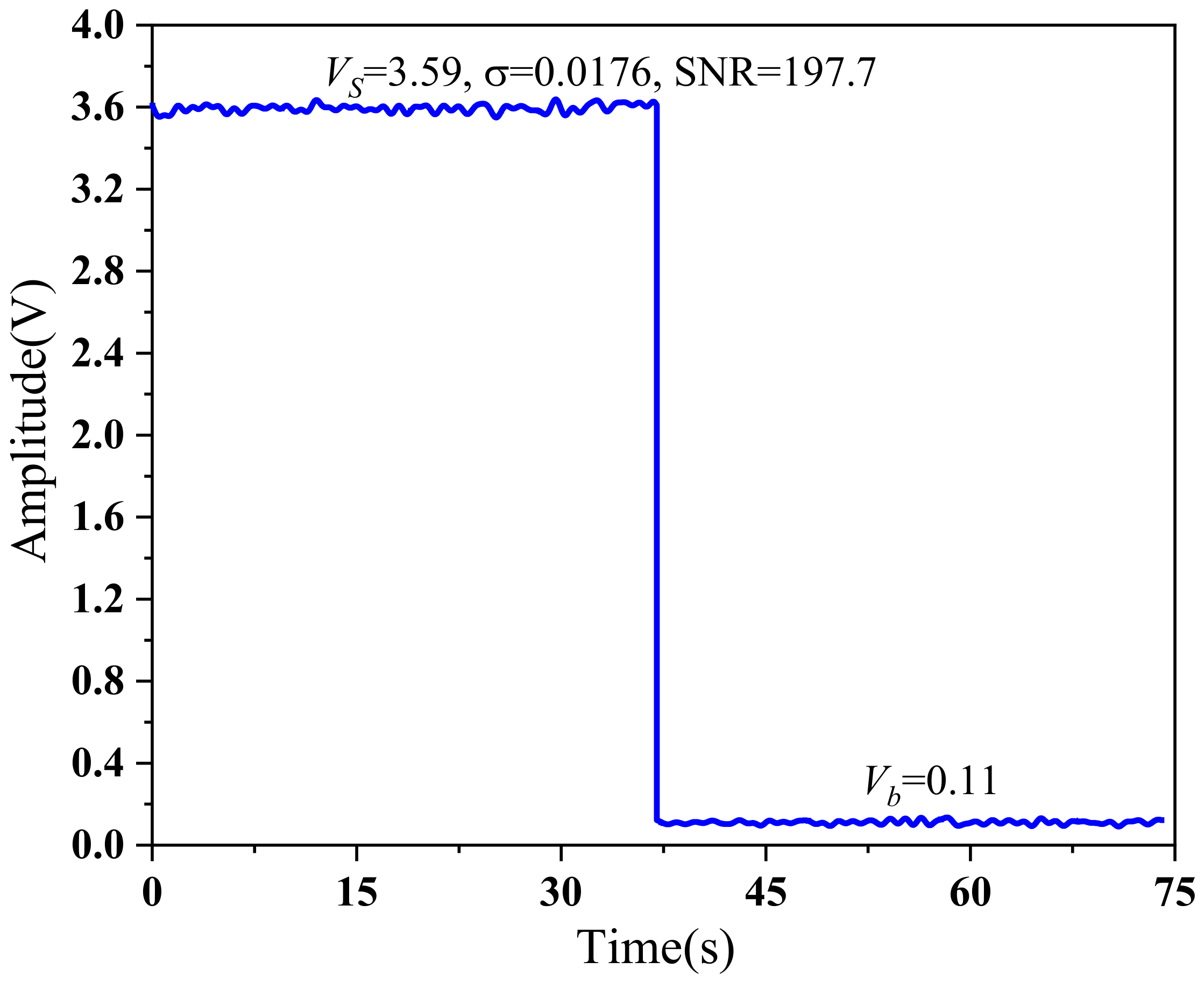
The SNR is the direct parameter that shows the performance of the LHR. The heterodyne signal and background signal (without sunlight input) were gathered before spectra measurement, and the SNR was 197.7 after being averaged 12 times (the SNR was about 57 without being averaged), as is shown in
Figure 11. The capability ensured the high-quality data of spectra.
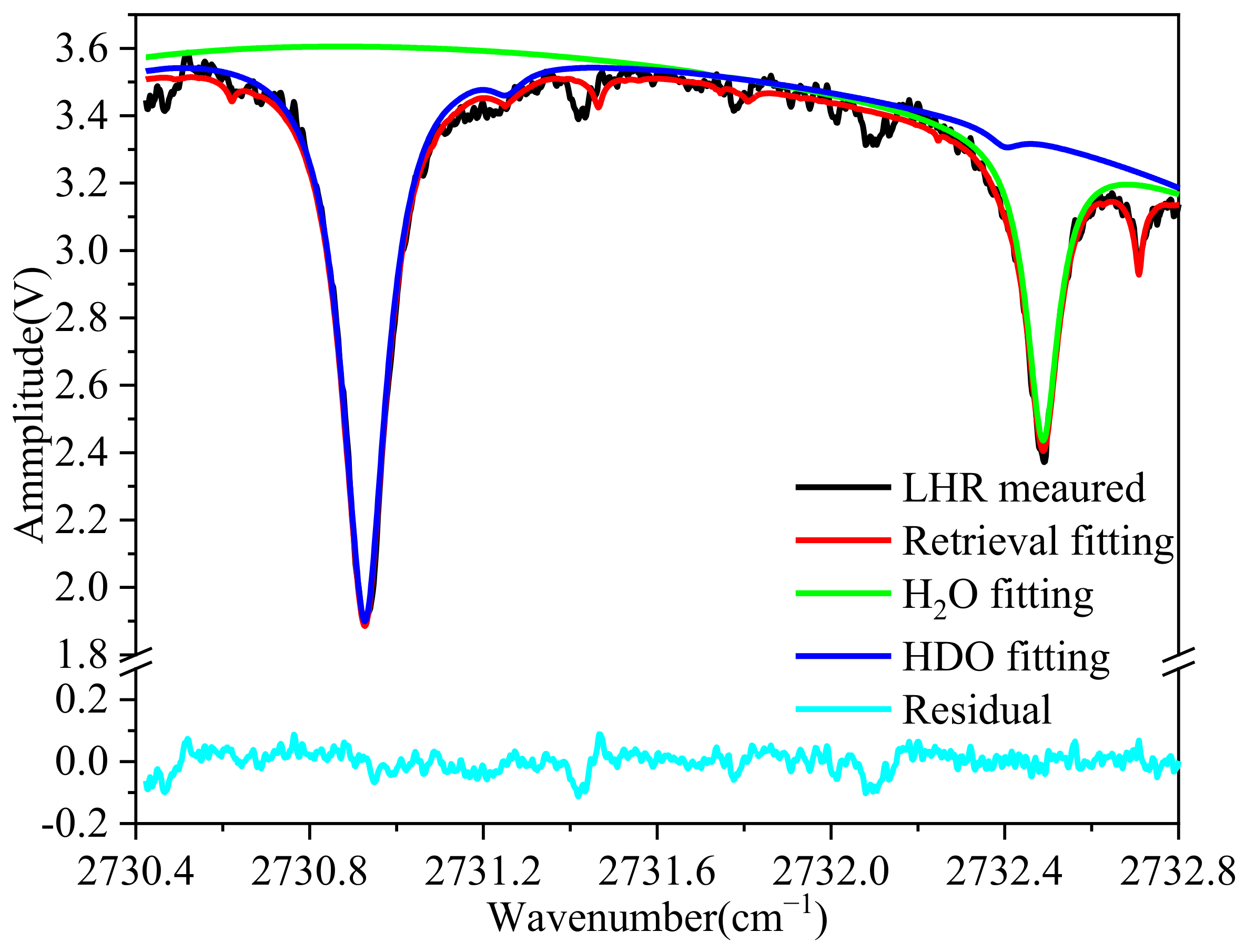
The OEM approach resulted in a more accurate fit to the measured spectrum. The absorption spectra of HDO and H
2O were obtained respectively during the retrieval. One of the measured and retrieved fitting spectra is shown in
Figure 12: the blue line is the fitted spectrum of HDO and the green line is the fitted spectrum of H
2O, and the red line is the synthetic spectra of retrieval fitting. The residual was less than ±0.1 V.
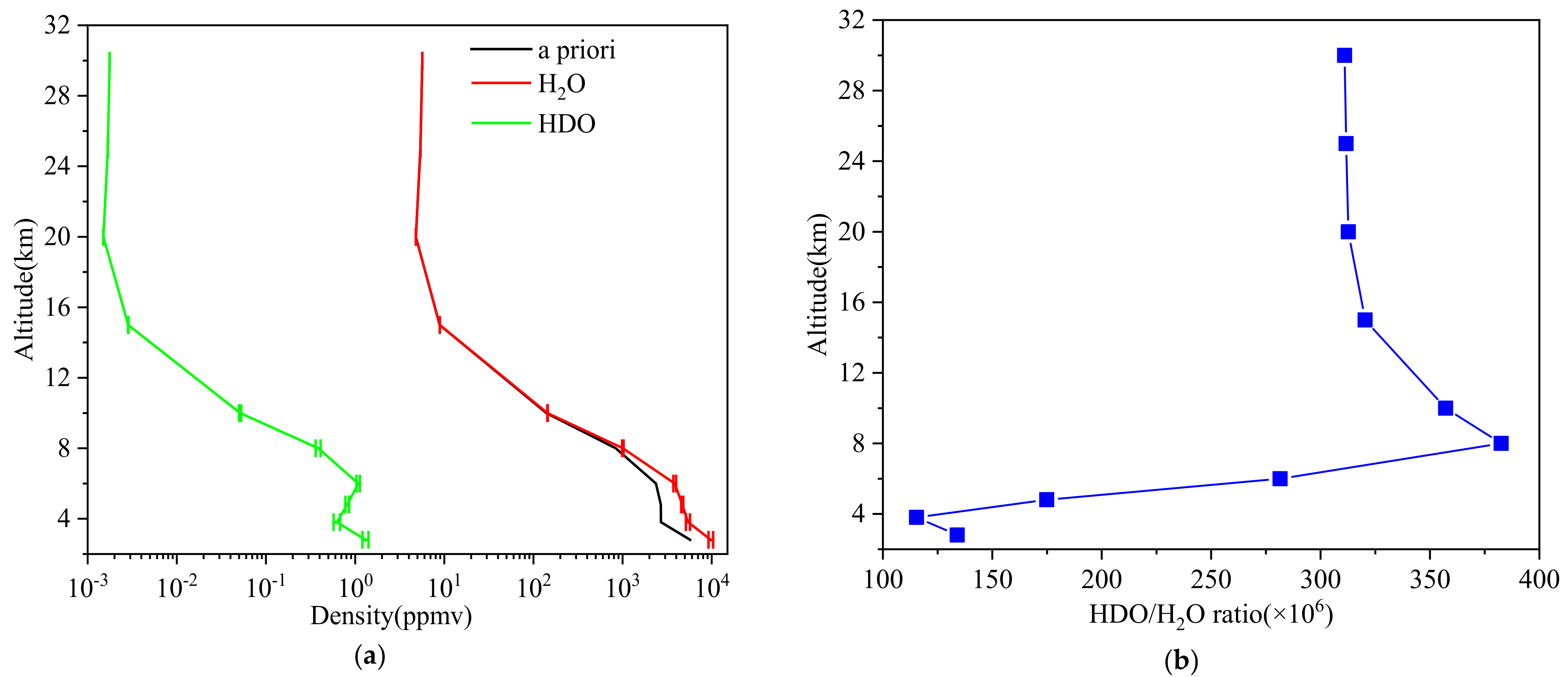
The retrieved profiles and their variations of H
2O and HDO, as well as the a priori profile from 2 August, are shown in
Figure 13. Although the retrieved profiles and their variances were not accurate enough, they still provided meaningful information about the measurements and the progress of the retrieval.
The retrieved profiles indicate that the measurements provide information on HDO and H2O distributions in the atmosphere below 10 km. However, in the upper atmosphere, the densities of HDO and H2O were significantly lower, and the LHR was not sensitive enough to detect them, as a result, the retrieved values in this range were almost identical to the prior profiles. The results suggest that the profiles of H2O and HDO could be retrieved in the lower troposphere based on LHR with higher sensitivity and a more comprehensive retrieval algorithm. The results suggest that it may be possible to retrieve the profiles of H2O and HDO in the lower troposphere using an LHR with increased sensitivity and a more comprehensive retrieval algorithm.
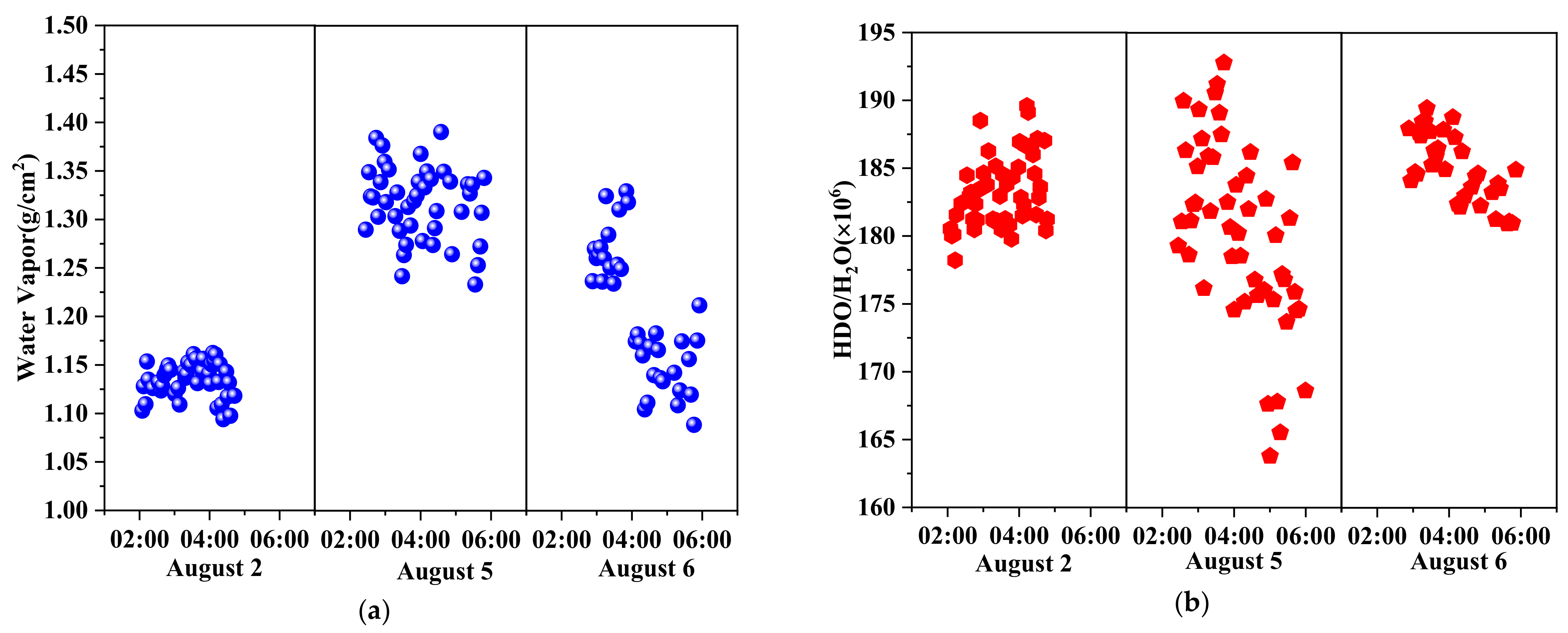
H
2O column density and HDO/H
2O ratio on 2, 5 and 6 August are shown in
Figure 14. Measurements were suspended due to cloudy and rainy conditions on 3 and 4 August. During the experimental campaign, the column density of H
2O was 1.07~1.4 g/cm
2 and the HDO/H
2O ratio in Golmud was 163 × 10
−6~193 × 10
−6. More specifically, the daily average H
2O column density for three consecutive days was 1.14 g/cm
2, 1.32 g/cm
2 and 1.20 g/cm
2, and the HDO/H
2O ratio was 185.05 × 10
−6, 180.20 × 10
−6, and 183.27 × 10
−6 respectively. The measured HDO/H
2O ratio was much lower than VSMOW, with a δD value of −476‰~−380.5‰, and the average δD over three days was approximately −413‰. As a reference, the average δD retrieved based on GOSAT data in June, July and August from 2009~2011 around Golmud were approximately −350‰ [
16], with a relative difference of ~18% to our results. Not only do the sensitivity of the LHR and the precision of parameters in the retrieval algorithm contribute to the differences, but the long-term and wide-range data averaging of satellite data could also be another significant factor. For a better understanding of the variations in atmospheric water vapor and its isotopes, the detailed analysis of water vapor density and the fluctuation of the HDO/H
2O ratio in Golmud will be presented in the next subsection.
5. Conclusions
The laser heterodyne radiometer is a powerful instrument used to obtain high-resolution solar spectra transmitted through the atmosphere. Despite its small size, it provides convenience for a wide range of atmospheric measurements. The self-built 3.66 μm LHR was successfully operated in Golmud in August 2019. The atmospheric H2O and HDO spectra were obtained using a new retrieval approach based on the optimal estimation method with LBLRTM as the forward model. Then, the column density of H2O and the ratio of HDO/H2O were investigated. The column density of H2O was 1.07~1.4 g/cm2 and the HDO/H2O ratio in Golmud was 163 × 10−6~193 × 10−6 during the experiment.
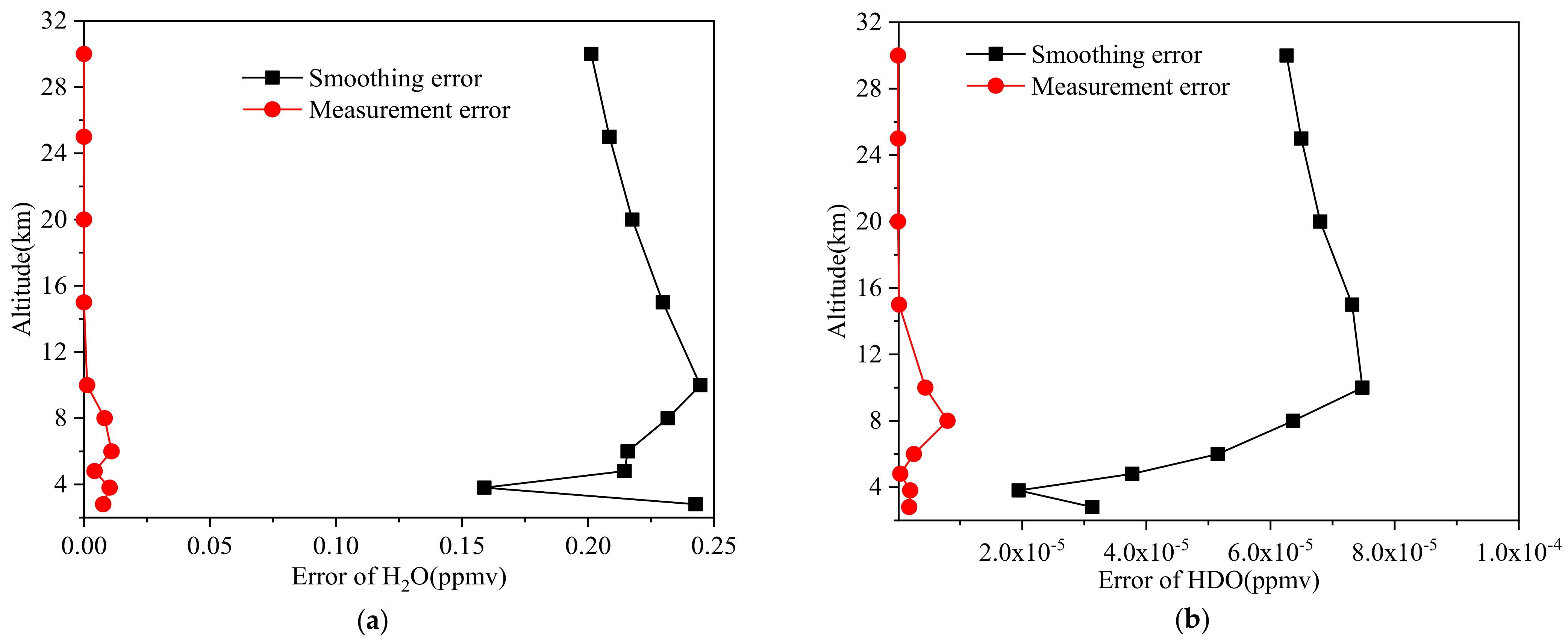
The analysis of the altitude grid optimized the better height spacing during the retrieval, the refined height layers reduced the redundant information. The retrieval errors were also analyzed in this work; the results indicate that the error in this work is mainly composed of smoothing error and measurement error, and the smoothing error is significantly higher than the measurement error. The retrieval error is related to the sensitivity of the laser heterodyne radiometer and the height distribution of water vapor and its isotope.
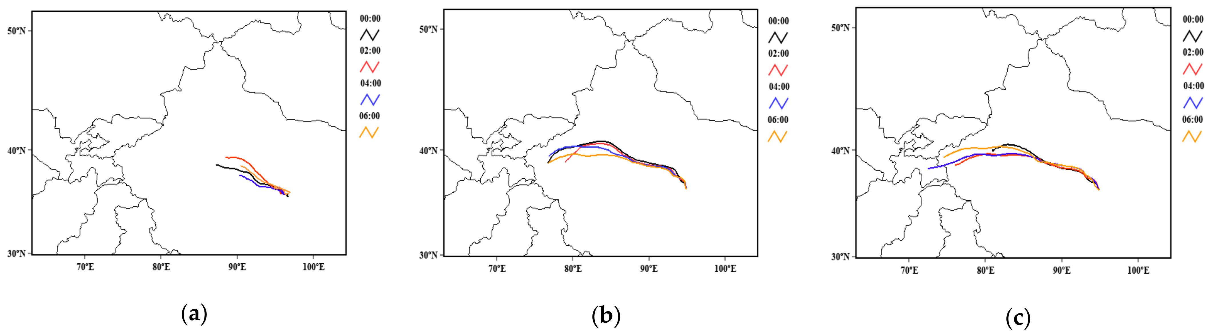
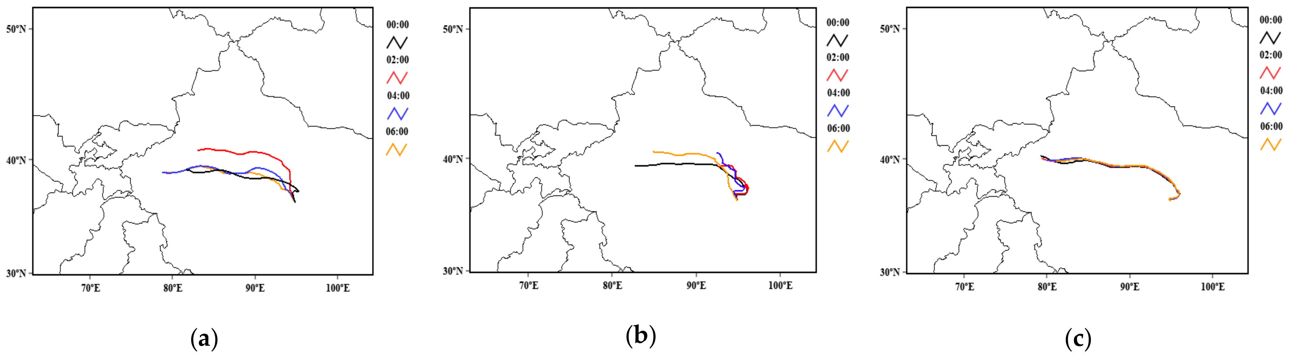
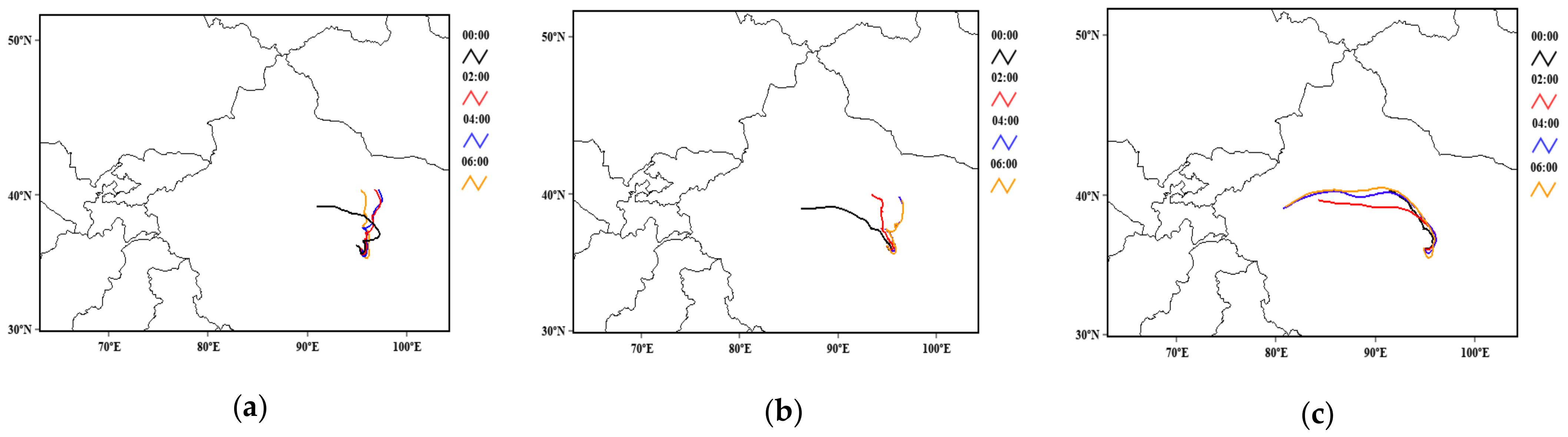
For a better understanding of the relationship between H2O (HDO) density and atmospheric motion, the research adopted backward trajectory analysis. Although the observations were not sufficient, the results indicate that the original location of airflow and the pathways influence the density of H2O and its isotopic abundance.
Therefore, the LHR can realize the measurements of column water vapor and isotopic ratio, and has the potential to retrieve H2O and HDO profiles in the lower troposphere. If long-term observation is carried out on the concerned sites, the variation regularity, sources and sinks of water vapor isotopes, and their relationship with atmospheric circulation can be further investigated. Recently, we have been working on improving the performance of the device. If possible, we plan to conduct long-term measurements in the TP or NW to gather more information on the abundance of HDO and environmental changes in this area. The study can help to gather data on atmospheric water vapor isotopes and improve the understanding of atmospheric circulation.


 ,
, 


