Article

Coupling the Calibrated GlobalLand30 Data and Modified PLUS Model for Multi-Scenario Land Use Simulation and Landscape Ecological Risk Assessment

1
School of Water Conservancy and Transportation, Zhengzhou University, Zhengzhou 450001, China
2
School of Architecture, Zhengzhou University, Zhengzhou 450001, China
3
Department of City and Regional Planning, University of Pennsylvania, Philadelphia, PA 19104, USA
*
Author to whom correspondence should be addressed.
Remote Sens. 2023, 15(21), 5186; https://doi.org/10.3390/rs15215186
Submission received: 20 September 2023 / Revised: 21 October 2023 / Accepted: 24 October 2023 / Published: 31 October 2023

Abstract

:
Rapid economic growth and urbanization have significantly changed the land use distribution and landscape ecological structure, which has a profound impact on the natural environment. A scientific grasp of the characteristics of land use distribution and its impact on landscape ecological risk is a prerequisite for sustainable urban development. This study aimed to calibrate GlobalLand30 data using the normalized difference impervious surface index (NDISI) obtained from Landsat images, thereby providing a more precise foundation for land simulation. Additionally, it sought to improve the accuracy of the patch-generating land use simulation (PLUS) through parameter sensitivity analysis. Building upon this, the research also simulates future land use in Beijing. Lastly, this study introduced an LER index to assess ecological risk in the current and future urban landscapes. The results showed that the GlobalLand30 data were calibrated and PLUS model accuracy was improved to more than 86%. The accuracy of the modified PLUS model based on a Morris sensitivity analysis was increased, and the kappa coefficients were increased by approximately 3%. The results of the multi-scenario simulation showed that under the SSP126-EP scenario, future land use in Beijing could balance urban development and ecological protection, and thus would be more suitable for sustainable development. In the other two scenarios, ecological land will be encroached by urban development. From 2000 to 2020, the degree of LER was generally lower, moderate, or higher, and the overall level of LER showed a downward trend continuing until 2100 in the SSP126-EG scenario. Future land use simulations and LER assessment under multi-scenarios could help decision makers develop multi-scale landscape protection strategies.

Graphical Abstract

1. Introduction

In the process of urbanization, the uncontrolled growth of cities has affected natural areas, creating a situation of conflict between “the people and the land”. The rapid expansion of urban space poses a real and potential threat to rainwater runoff, as it not only fundamentally alters regional substrate changes [1,2] but also exacerbates urban problems such as farmland loss, habitat destruction, water resource scarcity, floods and global warming [3,4]. Understanding the complex interactions between urban expansion and land use changes can clarify the connections between urbanization and land use [5,6]. Many studies have shown that the natural and economic aspects of cities have significant impacts on urban land use and land cover change (LUCC) processes [7,8], while LUCC is related to the overall environment, water resources, and regional sustainable development [9]. There are also many studies dedicated to investigating the subsequent impacts of LUCC changes in the context of urbanization, including environmental degradation [10], climate change [11], urban heat islands [12,13], and food safety [14].
With the development of urbanization, LUCC simulation prediction has gradually become a research focus. The Conversion of Land Use and its Effects at Small Regional Extent (CLUE-S) model has been combined with the Analytic Hierarchy Process to optimize land use and generate an acceptable and accurate land use classification tool [15]. Liu et al. [16] proposed the Future Land Use Simulation (FLUS) model based on traditional cellular automata (CA); the model has demonstrated higher simulation accuracy than CLUE-S and Artificial Neural Network-Cellular Automata (ANN-CA) and has been widely employed in land use pattern simulation research. Gong and Liu [17] studied the effects of six land use policies on the environmental sustainability of the oasis landscape in the Ganzhou region of Zhangye Oasis based on the FLUS model. Recently, the PLUS model was proposed by Liang et al. [18] as a raster-based patch generation land use simulation model. The PLUS model was proposed to address the limitations in both transformation rule mining and landscape dynamic change simulation strategies of the existing CA model.
Ecological risk refers to the potential for adverse impacts on the sustainability and stability of ecosystems caused by natural changes or human activities [19,20]. Landscape ecological risk (LER) assessment, as one of the most important research topics in ecological risk assessment, can reflect environmental issues caused by the interaction between nature and human activities and effectively guide the management and optimization of regional land use [21]. Ecological risk assessment of urban landscapes is currently carried out using a variety of methods, including mathematical models [22], statistical analysis based on indicators [23], and the use of tools such as remote sensing and GIS to obtain spatial data on urban landscapes, including LUCC and vegetation condition, to achieve landscape ecological risk assessment [24,25]. These approaches offer a comprehensive evaluation of the potential adverse effects of human activities on land use composition, structure, and function. Spatial visualization through fishing net construction on this basis can provide a more accurate spatial representation [26,27,28]. LER assessment based on land cover can reflect the negative impact of human activities on the interaction between the ecological environment and landscape pattern, and it is an important branch of LER assessment [29]. With the rapid development of dynamic modeling of land use change, LER analysis based on LUCC is gradually being applied [24]. The Markov-FLUS composite model was used to predict land use change under different scenarios in the study area, on the basis of which landscape ecological risk was assessed to help achieve regional ecological sustainability [30]. Ghosh et al. [31] applied Decision-Making Experimentation and Evaluation Laboratory (DEMATEL) and Analytical Network Processes (ANP) and CA-Markov models to assess urban ecological risks. The PLUS model combined with multiple linear regression and Markov chain models is also frequently used to predict future urban landscape patterns and assess LER [32,33,34].
Although there have been many researches on land use simulation based on the PLUS model, there is a lack of research on model accuracy. By using the traditional land use prediction model, the simulation results are not accurate. Therefore, this paper introduces the GLC30 data correction and parameter sensitivity analysis method based on the NDISI to improve the simulation accuracy of the PLUS model. The main purposes of the present study encompass the following: (1) to calibrate GlobeLand30 data by using the NDISI to refine the underlying data, thereby improving the PLUS simulations, (2) to determine the optimal range of neighborhood weight parameters based on a Morris sensitivity analysis and further determine the relevant parameters in order to modify the PLUS model, (3) to design the three future development scenarios (SSP245-ND, SSP585-EG, and SSP126-EP) based on the CMIP6 model and the experience of previous researchers and employ the PLUS model to simulate the land use distribution pattern in Beijing under multiple future scenarios, and (4) to construct the LER index and analyze the spatiotemporal characteristics of LERs in the past 20 years and evaluate future trends. Quantitative simulations of urban landscape ecology based on LUCC can provide suggestions for sustainable urban development.

2. Study Area and Data
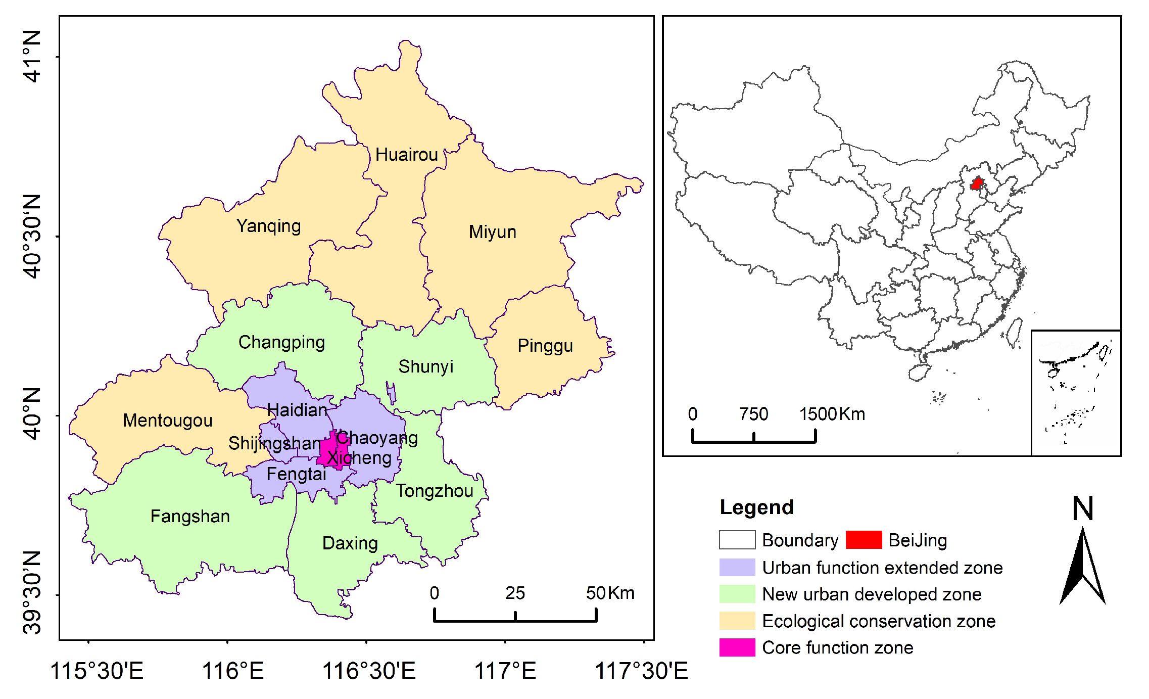
2.1. The Study Area

The study area was Beijing, the capital city of China (Figure 1). The past 20 years have seen rapid urban development, and the area of developed land in Beijing has increased from 1589.9 km2 in 2000 to 3475.5 km2 in 2020, gradually encroaching on the surrounding ecologically valuable land. Beijing has a continental climate with four distinct seasons: hot summers and cold winters. Located on the North China Plain, it is known for its gusty winds, especially in winter, which can cause sandstorms. Beijing is relatively dry, with limited rainfall and occasional droughts that affect the climate. The study area included all 16 districts and counties in Beijing distinguished according to the administrative divisions in the statistical yearbook of the National Bureau of Statistics as the core function zone (CFZ), the urban function extended zone (UFEZ), the new urban developed zone (NUDZ), and the ecological conservation zone (ECZ) [35].

2.2. Data

The ground cover data comprised a global 30 m ground cover dataset developed by China and donated to the United Nations in 2020 (GlobeLand30 Datasets, including three years, 2000, 2010, and 2020 (http://www.globallandcover.com/home.html?type=data, accessed on 1 September 2022)). Population data were taken from UN-calibrated data for 100 m countries. The data for the three years used in this study were resampled to obtain 30 m population size data in units of people. GDP data were sourced from the Natural Resources and Environment Center, Chinese Academy of Sciences (http://www.resdc.cn/Default.aspx, accessed on 1 September 2022). The road network data were from OpenStreetMap. Meteorological data were obtained from the China Meteorological Network. DEM data were sourced from NASA SRTM 30 m elevation data.
The data of each index used for Beijing are shown in Table 1.

3. Methodology

Figure 2 shows the workflow of this study. Firstly, the GLC30 land use data were calibrated based on the NDISI. Secondly, the optimal neighborhood weight parameters are determined by Morris sensitivity analysis and the accuracy is verified based on the actual land use. On this basis, the PLUS model and scenario design are used to predict future land use distribution under multiple scenarios. Finally, the LER index was constructed to analyze the landscape ecological risk in the recent 20 years and future multi-scenarios.

3.1. The Modified PLUS Model

3.1.1. The PLUS Model

The PLUS model is a raster-based patch generation land use simulation model that uses a CA with random seeds to simulate the generation of new land use patches by obtaining the relationship between land use type change and driving factors and mining land use type change rules [18]. In this study, remote sensing data of land use in China are used as the main data, and climate and environmental data, socio-economic data and constraints are input into the PLUS model as driver data. The model consists of two modules: the land expansion analysis strategy (LEAS) and the CA model based on multi-type random patch seeds (CARS). The LEAS works by extracting the fraction of each type of site expansion between the two land use changes and sampling from the increased fraction. The random forest classification (RFC) algorithm is used to mine the driving factors of various land uses individually to obtain the development probability of each type of land use and the contributions of such drivers to land expansion in this period [18]. The RFC algorithm extracts random samples from the original dataset and finally determines the P i , k d that appears in the i th cell of the kth land use type. The probability is expressed as follows:
P i , k d x = n = 1 M I = [ h n x = d ] M ,
where d takes the value of 0 or 1. If d = 1, this means that there are other land use types transformed into k land use types; if d = 0, this means that the land use type can be transformed into other land use types, except k . The term x is a vector consisting of several driving factors. Function I is the indicator function of the set of decision trees; h n x is the prediction type of the nth decision tree of vector x , and M is the total number of decision trees.
The CARS module is a scenario-driven land use simulation model that combines “top-down” (land use demand) and “bottom-up” (land use competition) effects. In the simulation process, land use demand influences local land use competition through an adaptive coefficient that drives the amount of land use to reach future demand. To predict the patch evolution under different land use scenarios, the PLUS model employs a random seed generation mechanism based on a decreasing threshold for multiple classes of patches. Using the Monte Carlo method, when the neighborhood effect of land use k is zero, the probability surface O P i , k 1 , t for each land use type is as follows:
O P i , k 1 , t = P i , k i × r × μ k × D k t i f   Ω i , k t = 0   a n d   r < P i , k i P i , k i × Ω i , k t × D k t a l l   o t h e r s ,
where r is a random value in the range of 0–1, μ k is the threshold value for generating new land use patches, D k t is an adaptive inertia coefficient indicating the effect of future land use demand on site type k , and Ω i , k t indicates the proportion of site type k in the neighborhood image element. If the new land type wins in a round of competition, a threshold decreasing operation is required for its result. The number of regression trees for the specific variable setting of the PLUS model was 50, and the sampling rate was taken as 0.01.

3.1.2. The Modified PLUS Model by Parameter Sensitivity Analysis

The neighborhood factor weight in the PLUS model is an important parameter affecting the PLUS simulation, and its value ranges from 0 to 1. Compared with using land expansion capacity to represent neighborhood weights [38], the introduction of a parametric sensitivity analysis [39] to determine the range of weight parameters and then further debug can effectively improve the simulation accuracy. Parameter sensitivity analysis is a standard method for uncertainty analysis in remote sensing and in ecological and hydrological modeling [40]. Morris’ calculation formula is as follows:
S = i = 1 n Y i + 1 Y i Y 0 P i + 1 P i / n ,
where S is the sensitivity discriminant; Y 0 is the accuracy verification result when the parameter is at the initial value; Y i is the accuracy check result of the ith simulation; Y i + 1 is the accuracy check result of the i + 1 t h simulation; P i is the relative percentage change in the parameter values involved in the calculation at the ith simulation compared with the initial value; P i + 1 is the relative percentage change in the parameter values involved in the calculation at the i + 1th simulation compared with the initial value. Based on the Morris screening method to rank the sensitivity of each land type according to S values, the disturbance range in this study was ±100% by perturbing the parameters of cultivated land, woodland, grassland, water bodies, built-up land, and unused land with a step size of 20%. Since the range of neighborhood weights for each land use type is [0,1], their initial values were all taken as the same value of 0.5. Referring to previous studies [18,38,41], we determined the range of neighborhood weights for each type of land use: [0.7–0.8] for cultivated land, [0.2–0.3] for woodland, [0.5–0.6] for grassland, [0.2–0.3] for water bodies, [0.9–1.0] for built-up land, and [0.1–0.2] for unused land. Parameter debugging tests were conducted, and the parameter with the highest simulation accuracy was finally determined as the model neighborhood weight value.

3.1.3. Model Validation

In order to effectively simulate future land use, we used the kappa coefficient [34] and FoM values [42] to verify the applicability of the PLUS model. The kappa coefficient is the most commonly used way to test the accuracy of the image classification, and the consistency test is performed by calculating the confusion matrix. Assuming that the image element is and the total observation value of the image element in the confusion matrix is p , the kappa coefficient formula is as follows:
k a p p a = P a P b P c P b ,
where P a is the proportion of correct simulations and P b is the expected proportion of predicted simulations. P c is the ideal simulation value, generally defined as 1. A result value of 1 indicates complete consistency in land use between the two periods; a value greater than 0.75 indicates a high degree of consistency between the resultant maps and the ground reference information; a value of 0.4 < K < 0.75 indicates moderate consistency, and a value of less than 0.4 indicates very poor consistency.
F o M quantitatively tests the accuracy of simulation at the cellular scale, and assesses the accuracy of the simulation results by judging the results of the ratio between the intersection of the actual land use change and the predicted change and the concatenation of the two, with a range of values, with larger F o M values indicating higher accuracy, but practical tests have found that most of the results are within 0.3 [43]. The expression is given below:
F o M = B A + B + C + D ,
where A is the error region where the actual change is unchanged but the simulation is unchanged; B is the region where the actual change is changed and the simulation is also changed; C is the region where the direction of the actual change and the simulation change do not coincide; and D is the error region where the actual change is unchanged but the simulation is changed.

3.2. GlobalLand30 Data Calibration

At the global scale, GlobalLand30 data have an overall accuracy of over 80% [44]. However, at the urban scale, a decline in accuracy occurs due to individual extraction with different reclassification schemes [45]. To improve the classification accuracy, especially for impervious surfaces, this study calculated an impervious surface index for Beijing and determined the appropriate threshold value by combining these indices with remote sensing images to obtain the N D I S I index of impervious surface with high accuracy at the urban scale [46,47]. Using Landsat images of 2010 and 2020 as data sources, the spectral index method was employed for N D I S I index calculation and threshold determination to extract impervious surface information in the study area using the following equations:
N D I S I = T I R M N D W I   +   N I R   +   M I R 1 3 T I R   +   M N D W I   +   N I R   +   M I R 1 3 ,
where N D I S I is the normalized differential impervious surface index; N I R , M I R 1 , and T I R are the reflectance values in the near-infrared, mid-infrared, and thermal infrared bands of the remotely sensed images, respectively. M N D W I is the modified normalized water body index. We first determined if there were values for N D I S I and GlobalLand30 land use. If there was a value, the calibrated result was a water body when the GlobalLand30 image was a water body; otherwise, the result was the N D I S I value. If there was no value, the calibrated result image was the GlobalLand30 value.

3.3. Land Use Prediction and Multi-Scenario Design

The Markov prediction model uses a Markov chain to analyze the occurrence and the probability of a transfer [48] and to predict future trends based on the probability values. Simulation of the process predicts the probability of geographical events with the characteristic of no posteriority. Assuming that there are n possible outcomes for a certain event corresponding to states E 1 , E 2 ,… E n , and the probability of state transfer from state E i to state E j is P i j , the simulated prediction formula for land use change is as follows:
S t + 1 = P i j · S t       0 P i j 1 i , j   i s   a n y   n u m b e r   o f   1,2 , , n j = 1 n P i j = 1 i , j   i s   a n y   n u m b e r   o f   1,2 , , n ,
where S t denotes a certain land use type in the image element at epoch t; S t + 1 denotes the land use type of the image element at epoch t + 1 ; and P i j is the state transfer probability matrix of different land use types.
The Coupled Model Intercomparison Project (CMIP6) has proposed a series of scenarios for climate model simulations to study the impacts under different climate change conditions. SSP1 to SSP5 represent five pathways for sustainable development, moderate development, regional development, uneven development, and conventional development, respectively [49]. In the land use projections, three land development simulation scenarios were designed by combining future development patterns with typical SSP scenarios under CMIP6 [38,50,51]: SSP5-8.5 with an economic growth scenario (SSP585EG), SSP1-2.6 with an ecological protection scenario (SSP126EP), and SSP2-4.5 with a natural development scenario (SSP245ND).
The SSP245ND scenario embraces a track where historical development patterns serve as a basis for projecting future socio-economic development, while simultaneously maintaining the existing trend in land use. On the other hand, the SSP585EG presents a high-speed development model taking into account the economic cost associated with extensive use of fossil fuels. This study augmented the transfer probability of cultivated land, woodland, and grassland to built-up land by 20% to maximize economic gains. In sharp contrast, SSP126EP embodies a vision of green and sustainable development, with a sharp focus on ecological preservation. It deliberately curtails the expansion of built-up land by significantly reducing the transfer probability of cultivated land and woodland to impervious surfaces by 50%, along with a 30% reduction in the conversion probability of grassland and water bodies to built-up land, all encapsulated within the transfer probability matrix.

3.4. The Landscape Ecological Risk Index

Based on the area proportion of land use types and the landscape loss index R i , this study constructed a LER index [52]. The formula is as follows:
L E R i = i = 1 N A k i A k R i ,
where L E R i is the LER index of LER assessment unit i ; A k i is the area of landscape type i within the k i sample unit; A k is the area of the kth sample unit; R i is the landscape loss index of landscape type i , which is determined by the landscape disturbance index E i and the vulnerability index F i of each landscape type. The calculation formula is as follows:
R i = E i × F i ,
E i = a C i + b N i + c D i ,
where E i is the landscape disturbance index calculated by the landscape fragmentation degree C i , the landscape separation degree N i , and the landscape advantage D i construction, where a , b , and c are the weights of the corresponding landscape indices, and a + b + c = 1 . Based on existing research results and actual situations [27,53], the values were assigned as 0.5, 0.3, and 0.2, respectively. F i is the landscape vulnerability index; based on existing research results [26], this study assigned values to six types of landscapes using an expert scoring method, i.e., assigning values 6, 5, 4, 3, 2, and 1 to unused land, water bodies, cultivated land, grassland, woodland, and built-up land, respectively. Finally, the indices were obtained through normalization as 0.29, 0.24, 0.19, 0.14, 0.10, and 0.05. The natural breakpoint method was used to divide the LER index values of risk areas. To better identify the ecological risk changes in the landscape and to uniformly evaluate the ecological risks for different periods, the data for other periods were classified into five levels using the 2020 classification interval: lowest level ( E R I 0.018 ), lower level ( 0.018 < E R I 0.024 ) , moderate level ( 0.024 < E R I 0.029 ) , higher level ( 0.029 < E R I 0.035 ) , and highest level ( E R I > 0.035 ) . To explore the spatiotemporal distribution characteristics of LERs in Beijing, we employed the ArcGIS10.2 fishing net tool to construct a land use data grid of 2   k m × 2   k m divided into 4367 evaluation units. We calculated the LER index values for each evaluation unit using Fragstats4.2 and then performed a visual analysis.

4. Results

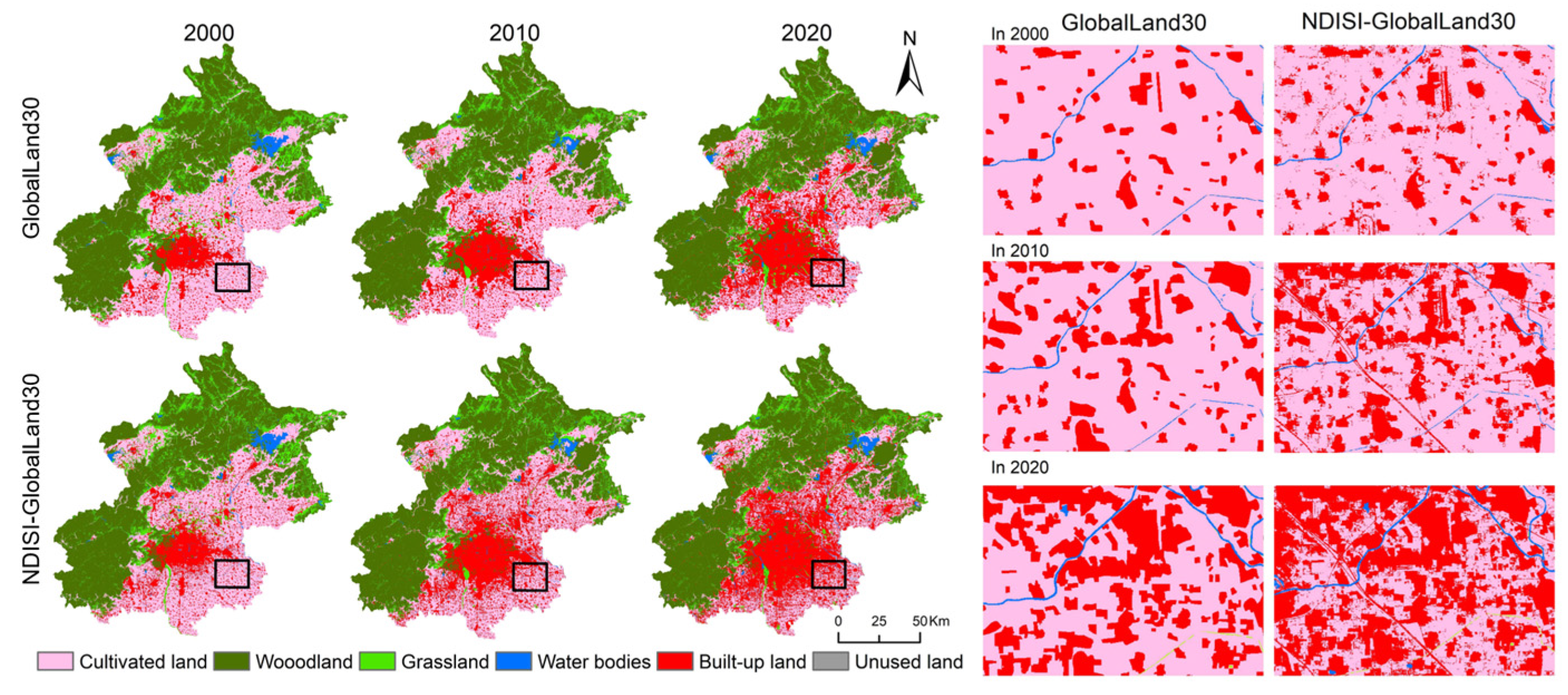
4.1. Calibrated GLC30 Data for PLUS Simulation

Figure 3 shows the land use of Beijing before and after calibration for 2000, 2010, and 2020. The trend of built-up land expansion in Beijing over the past 20 years is extremely clear, with growth expanding from the suburban areas of Chaoyang and Haidian into Tongzhou, Changping, and other distant suburban districts and counties. The junction area between Chaoyang District and Tongzhou District were largely scattered and independent. The calibrated results showed that independent township residential areas had higher connectivity, and some small and previously unrecognized impervious surfaces were identified. In the time series, the key areas were still dominated by scattered settlements in 2000, and the urbanization process had not yet advanced to these locations. By 2020, 15.82% of the cultivated land was transformed into built-up land, and southeast Beijing was highly urbanized.
Table 2 presents the results of PLUS simulation accuracy validation before and after calibration of GLC30 data in 2010 and 2020. The overall accuracy of simulations without calibration were 0.814 and 0.825 in two terms, respectively. After calibration based on the NDISI, the overall accuracy of the simulations increased to more than 0.86 in 2010, with an improvement of approximately 4%. The increase in accuracy indicated that the calibration of GLC30 data by the NDISI improved the PLUS simulation.
Figure 4 shows the land use changes in the four functional zones in Beijing during the past 20 years. Cultivated land was mostly in the NUDZ and ECZ areas that have experienced a significant decrease in the last 20 years, totaling 2022.09 km2. Notably, only 0.001% of the cultivated land in CFZ would remain by 2020. In 2020, woodland accounted for 62.9% of the total area in the ECZ, presenting an increase of 2.2% from 2000 to 2020 due to the successful implementation of afforestation policies in this ecological conservation zone. Grassland was concentrated in the ECZ region as well as woodland, and the grassland in the region decreased by 3.72% between 2000 and 2020, becoming transformed into woodland and built-up land. The built-up land showed a significant growth trend and was distributed in all functional zones, with the most dramatic increase in the NUDZ with a growth rate of 152%. By 2020, the proportion of built-up land in the CFZ reached 94% with rapid urbanization and construction. Most water bodies were distributed in the ECZ, representing 3.03% of the regional area in 2000, and this declined to 1.97% in 2020. Unused land was largely distributed in the ECZ and NUDZ regions, comprising 0.02% of Beijing’s total area in 2020.

4.2. Simulation after Modifying the PLUS Model

Figure 5 shows the simulation of 12 parameter combinations in 2020, the ranges of which were determined by the Morris screening method. By tuning the simulation with different parameter combinations in the above ranges, it was found that the best simulation results were achieved at 0.7, 0.3, 0.5, 0.2, 1.0, and 0.2 for cultivated land, woodland, grassland, water bodies, built-up land, and unused land, respectively, at which the overall accuracy reached 87.6% with a kappa coefficient of 0.812. The rest of the parameter combinations were simulated with the overall accuracies floating in the range of 0.86–0.87, and the kappa coefficients were fluctuating between 0.195 and 0.21. kappa coefficient fluctuates between 0.195 and 0.21.
Table 3 shows the comparison of the accuracy between the two simulation approaches. In this study, the parameters were first set according to the historical scenario; the kappa coefficients were calculated to be 0.797 and 0.8 for 2010 and 2020, and the F o M values were 0.155 and 0.18. Subsequently, the modified model was validated and the overall accuracy was found to be the lowest at 0.867; the kappa coefficients were 0.826 and 0.814 for 2010 and 2020, and the lowest F o M value was 0.21. The comparison in the table shows that the kappa coefficient was improved by 2.9% and 1.4% after correction and the F o M value was improved by more than 3%. This demonstrated that determining the weights based on Morris sensitivity analysis parameters can effectively improve the accuracy of PLUS simulation. The high-accuracy simulation results were visualized to obtain the validation comparison graph shown in Figure 6. Comparing the results of real and simulated sites in the two phases, the simulated results did not show substantial fluctuations with the actual status, and the land use structure was relatively stable. Specifically, the simulation accuracy of built-up land and water bodies was low, while the simulation results of woodland and grassland were better.

4.3. Land Use Simulation and Prediction under Multiple Scenarios

Figure 7 shows the contributions of 12 driving factors to the development of each type of land use were obtained from the analysis of LEAS. As shown in the figure, rainfall, DEM, and population have a significant influence on the distribution of water bodies, with the factor for rainfall reaching 23.79%. DEM, rainfall, and temperature are the strongest factors for cultivated land, at 11.28%, 9.92%, and 19.28%, respectively. The development of built-up land is primarily influenced by population, GDP, and DEM, with an influencing factor of approximately 14%. In addition, other driving factors such as rainfall, temperature, and distance have a more balanced effect on various land use types.
Future land use demand in Beijing for 2040–2100 under the SSP245-ND, SSP585-EG, and SSP126-EP scenarios was predicted using CMIP6 and the Markov chain method in the PLUS model (Figure 8). There were significant differences in the quantity of each land type under the three scenarios. In the SSP245-ND scenario, the area of built-up land increases rapidly and the cultivated land decreases accordingly. The area of built-up land increases from 3475.47 km2 to 5679.69 km2 during 2020–2100, and the new area accounts for 92.44% of the loss of cultivated land, indicating that the vast majority of the loss of cultivated land is due to occupation by built-up land. In the SSP585-EG scenario, the percentage of built-up land changes most dramatically, reaching 86.8%. In contrast, the cultivated land area decreases by 66.42%, woodland by 7.1%, and grassland by 5.8%. Due to the limitations of undevelopable water bodies and ecological replenishment, the area of water bodies has also been greatly improved, increasing by 70.59% and enhancing the landscape pattern of the city. Under the SSP126-EP scenario, the amount of cultivated land would have the lowest reduction rate compared to other scenarios due to the weakening of the conversion efficiency of cultivated land and woodland to built-up land. Compared with the SSP585-EG in the same period, 776.76 km2 more cultivated land can be retained, and the rate of loss is slowed by 38.7%. Only SSP126-EP among the three scenarios can ensure that the proportion of basic farmland is sufficient and would not be encroached upon, while woodland and grassland increase slowly, by 2% and 6.9%, respectively.
Figure 9 shows the spatial distribution of land use under multiple scenarios. Under the SSP245-ND scenario, the built-up land increases rapidly, concentrating in the central and southeastern parts of Beijing, and extending from the CFZ and UFWZ to the NUDZ. Woodlands, grasslands, and water bodies increase slightly, with woodlands and grasslands concentrated in the northwest, southwest, and northeast of the ECZ. Cultivated land shows a significant decrease and is constantly being encroached upon by built-up land. The SSP585-EG scenario shows a greater increase in built-up land and a significant increase in the distribution density of NUDZ, which basically coincides with the overall development direction of Beijing spreading from urban areas to the surrounding areas. In the SSP126-EP scenario, the rate of invasion by built-up land decreases. Ecological lands such as woodlands and grasslands show an increasing trend since woodlands are located in the mountainous areas in the west and northeast and thus are not susceptible to human activities. In addition, the development of areas with slopes greater than 25° is restricted, and there is the potential for afforestation. Water bodies also increase rapidly and thus have a significant effect on the enhancement of Beijing’s landscape.

4.4. Spatiotemporal Distribution Characteristics of Landscape Ecological Risks

From 2000 to 2020, the overall LER in Beijing was generally at a lower, moderate, or higher level, accounting for over 70% of the total area (Figure 10). The average LER indices for 2000, 2010 and 2020 were 0.0263, 0.0260, and 0.0258, respectively, indicating a downward trend. The areas of moderate level and below were largely distributed in the central plain and western mountain areas. The central plain is a concentrated area of built-up land, and urban development in this region is stable and not easily affected. The main types of land use in the western mountainous areas are woodland and grassland, types that are less affected by human activities and that are relatively stable, and thus, the degree of landscape fragmentation is lower. In the past 20 years, there has been an upward trend in the area of lowest level, with the proportion increasing from 6.8% in 2000 to 11.47% in 2020. The increase in area is primarily in urban functional extended zones and in some newly developed urban areas. The areas of higher and highest levels were concentrated in the north and southwest, with a wide area of cultivated land and water bodies within the region and weak stability. Most are located at the edges of urban development and are highly vulnerable to human activities. Between 2000 and 2020, the area of highest LER decreased by 53.08%. This is because with the continuous development of the economy, built-up land has significantly increased, constantly encroaching on cultivated land and developing from a disordered state to an ordered state, resulting in a significant improvement in the stability of the system in the central plain area.
The spatial distribution pattern of LER under the SSP126-EP was consistent with that from 2000 to 2020, and the LER was still dominated by lower, moderate, and higher levels (Figure 11 and Table 4). Compared with 2020, the area of lower and moderate levels increases by 23.35% and 10.45%, respectively, by 2100. The increased area is concentrated in the urban function extended zone that is dominated by built-up land. The land use development is more planned, and because the ecological protection scenario restrains the expansion of built-up land, this slows the increase in landscape fragmentation and separation in the urban fringe areas and thus enhances landscape stability. The areas of the highest level decrease most significantly, by 32.79% by 2100. The distribution pattern of ecological risk areas is changed under the SSP245-ND and the SSP585-EG scenarios, with the lowest, lower, and moderate levels dominating overall. Under these scenarios, land use changes are dominated by the expansion of built-up land, resulting in a significant reduction in the areas of the highest level. Compared with 2020, the area of the highest level under the SSP245-ND and the SSP585-EG scenarios decreases by 60.83% and 67.03% by 2100, respectively, with the reduction concentrated in the new urban developed zone on the central plain, the main construction land for future urban expansion in Beijing. In addition, under the SSP585-EG scenario, the area of the lowest level is the largest, increasing by 165% compared to 2020. Under this scenario, economic development is vigorously pursued, with the resulting loss of ecological land. The area of urban construction land increases and evolves from a disorderly state to an orderly state after several decades, so that the stability of the system gradually improves; the land in the central and southeastern regions develops regional stability, and ecological risk is greatly reduced.

5. Discussion

5.1. Comparison of Driver Contributions

Our study identified population, DEM, GDP, slope, rainfall, temperature and distance to roads at all levels as drivers to be analyzed. A large number of studies have highlighted that the human activities had the dominant driving role in land use changes, while built-up land was influenced by population, terrain (DEM), and climate (precipitation) [54,55,56], which is consistent with our study. However, a study showed that population and GDP have little effect on land use change in arid Africa [57].
To verify the impact of the driving factors on the study area, six factors (population, GDP, DEM, rainfall, temperature, and Euclidean distance to the highway) with the greatest impact on land development were selected for simulation and comparison based on the contribution values from 2000 to 2020. The simulation results showed that the overall accuracy was reduced by 0.9% and 0.7% when the six typical factors are used compared with the twelve factors; the kappa coefficient was reduced by only 0.1%, and the FoM value was also reduced by approximately 0.7%. Compared with the simulation using 12 driving factors, the overall accuracy has only slightly decreased. This indicates that when coupling the PLUS model simulation based on the GLC30 calibrated data and the sensitivity analysis method, selecting some of the drivers with larger contributions can achieve better land use simulation. When simulating land use in a large study area such as when He [58] studied the loss of natural habitats and endangered species caused by global urban expansion, efficiency can be improved by conducting land use simulations after the screening of driving factors. When the study area is large, the factors must meet the requirements of accessibility, spatial difference, consistency, correlation, and quantification. Selecting typical factors can rapidly achieve data preparation. In the PLUS model, the LEAS uses an RFC algorithm to explore the relationship between the growth of various land use types and multiple factors [18]. When using typical factor calculations, the algorithm traversal time is reduced, and the simulation efficiency is improved.

5.2. Strengths and Limitations

The PLUS model has been demonstrated to be an efficient model that provides more accurate simulation results [18]. In general, land use dynamics are complex and variable. Therefore, it is difficult for any simulation model to fully describe land use change [59,60,61]. The PLUS model’s mining framework of land use extension and conversion rules has temporal properties that can simulate the evolution of land use types and portray land change over specific time intervals. Compared to other models, it can also identify the driving factors of land expansion and predict landscape dynamics at the local level and can be coupled with multi-objective optimization algorithms [62]. The simulation results can better support planning policies to achieve sustainable development [63]. Under the SSP245-ND scenario, future land use maintains the current trend, resulting in continued urban expansion, increased competition with other land use types, and increased threat to woodland and water bodies. Under the SSP585-EG scenario, the growth rate of built-up land is as high as 83.92% due to socio-economic factors. This is the same trend as observed in the study by Wu et al. [38]. However, large-scale resource extraction and unrestricted built-up land expansion both accelerate the encroachment upon ecological land, thus increasing LERs. The SSP126-EP scenario improves socio-economic development and reduces the level of social inequality. In the current era of rapid growth of built-up land and prominent conflict between protecting cultivated land and securing development, it is necessary to balance the relationship between cultivated land protection and urban construction. The development of urbanization is carried out under the premise of ecological protection to reduce the LERs and achieve green sustainability.
The choice of the model driving factors and parameter settings is the main aspect that determines the simulation accuracy. In this study, the driving factors of PLUS simulations covered as many demographic, socio-economic, and climatic factors as possible, but there are still some factors that have not been fully considered. For example, in the future, the choice could be made toward more relevant changes in housing prices or distance to hospitals and schools. In addition, a parametric sensitivity analysis can effectively improve model simulation accuracy. Urban expansion is a very complex process that is not a simple linear relationship between population, economy, and urban land area [64]. The parameter values of any land use simulation model often require estimation for different application scenarios, and parameter variation can cause uncertainty in simulation results [65]. Parameter sensitivity analysis is an important step to improve model understanding and use [66], and its use in PLUS model simulations along with GLC30 calibrated data effectively improves simulation accuracy. Although the coupled model has not yet matured, it can still play a role in the development of land use simulation.
Land use change has been shown to be closely related to ecological risk [67], thus facilitating the analysis of the spatiotemporal distribution characteristics of LERs based on the relationship between LUCC and LER. The LER index is determined by the composition of landscape types and their vulnerability [26,68], and thus, different risk area changes with land use change. From a temporal perspective, the ecological risk of the landscape was generally lower, moderate, or higher during the period 2000–2020. With rapid economic development, urban construction encroaches on a large amount of cultivated land; development changes from disordered to ordered, and the system becomes more stable, making the overall LER show a decreasing trend. There is a continuous decreasing trend from 2040 to 2100, especially under SSP245-ND, where the lowest LER area reaches the maximum. From the spatial perspective, urban expansion and increased land fragmentation have become the main driving factors of higher LER values [69]. The LER in this study is lower in the central plain and the mountainous areas in the west and north, while the value is higher at the junction of the plain and mountainous areas. This is due to the fact that the junction comprises the edges of towns and cultivated land, and the continuous encroachment on cultivated land with the expansion of built-up land has resulted in a highly unstable system in the area.
The PLUS model coupled with LER index methods used in this study is not only applicable to the current study, but can also provide useful references for research in other fields, like GIS, remote sensing data processing, model improvement, land use change and ecological risk assessment to provide scientific support for decision making and have a wide range of potential applications.

6. Conclusions

This study considered Beijing as the research object, calibrated the GLC30 data based on the NDISI, modified the PLUS model by the Morris sensitivity analysis, and simulated the urban land use distribution of Beijing for 2040, 2060, 2080, and 2100. The LER index was established to assess the spatiotemporal characteristics of LERs in the past 20 years and to evaluate future trends. The results indicated the following.
(1)
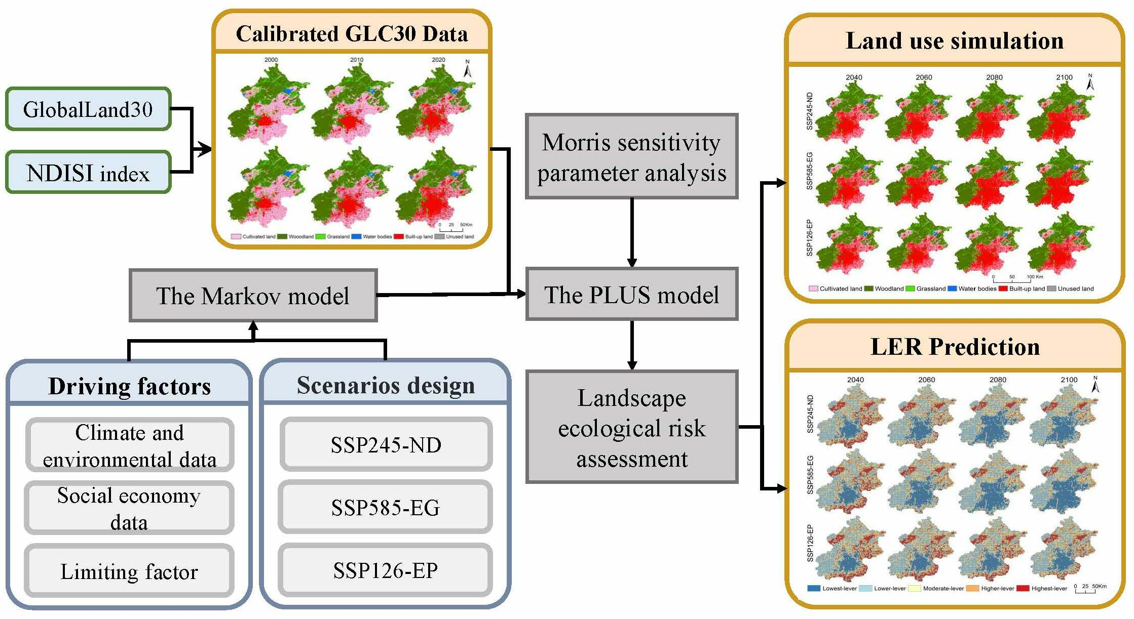
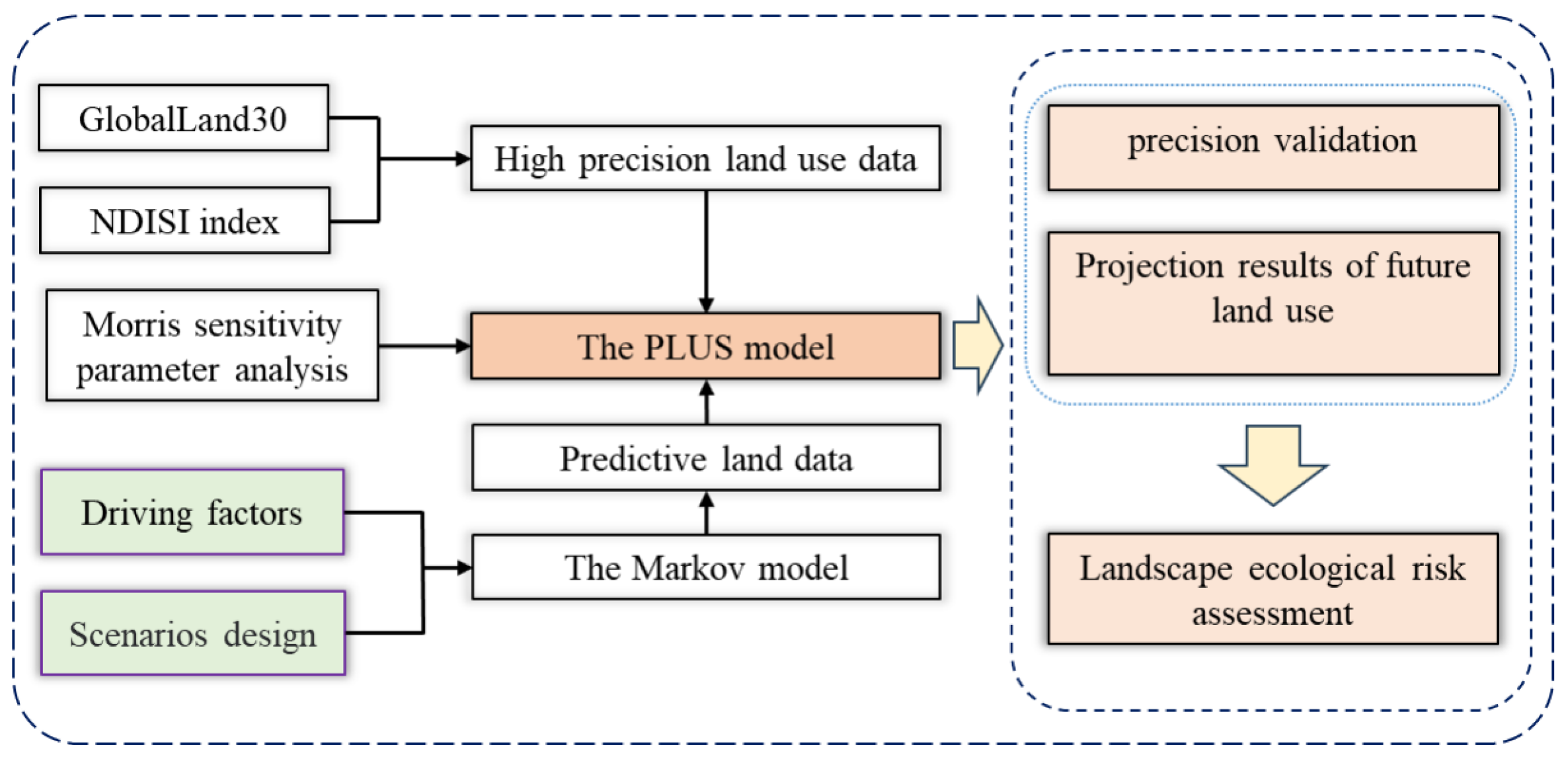
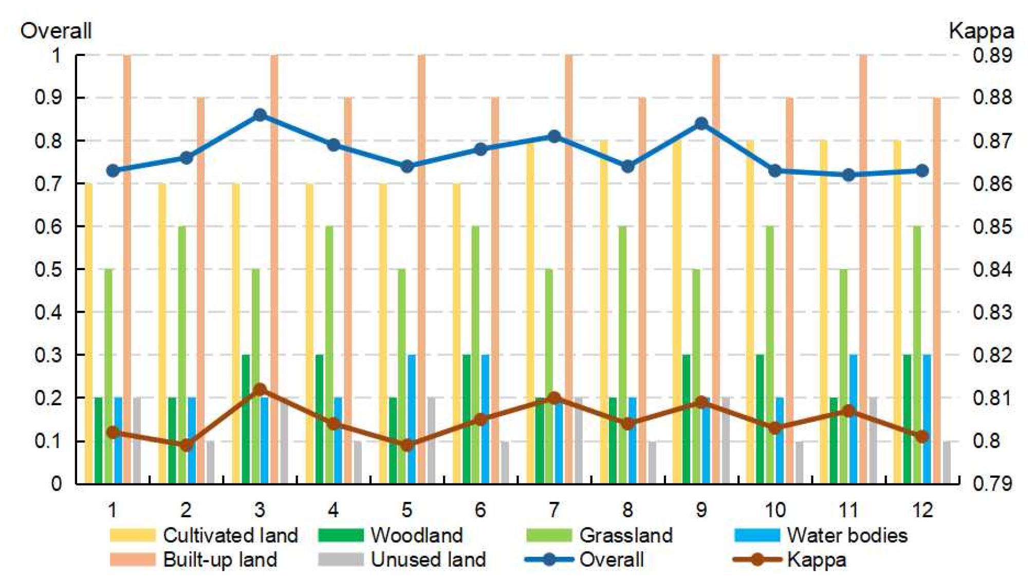
The impervious surface correction of GLC30 based on the NDISI significantly improved the connectivity of independent township settlements. The calibrated simulation accuracy was enhanced to greater than 0.86 based on PLUS simulation.
(2)
The modified PLUS model by the sensitivity analysis increased the kappa coefficient and the FoM value by more than 1.4% and 3%, respectively, and the overall accuracy reached 87.6%, effectively improving the accuracy of the PLUS simulation.
(3)
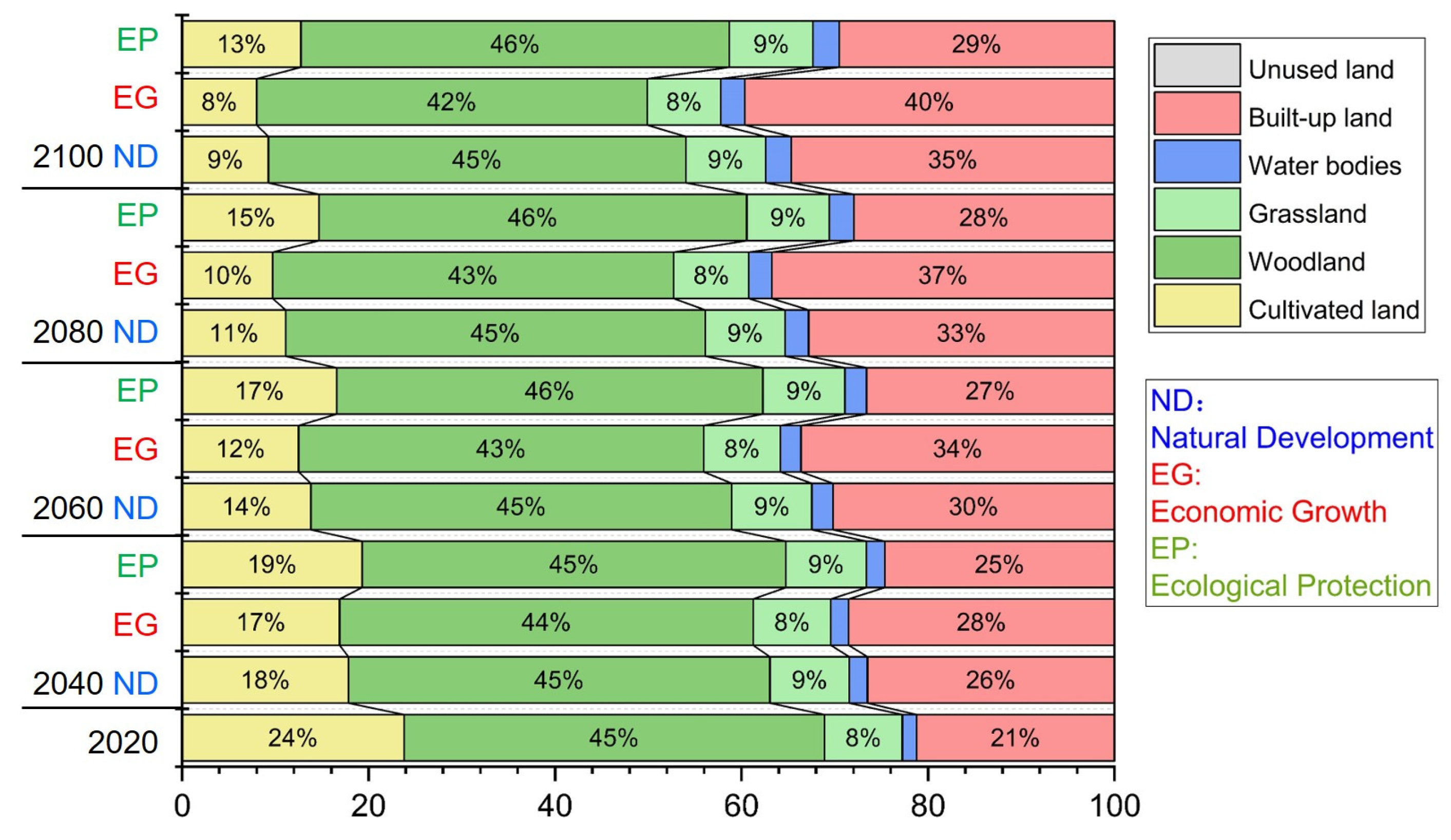
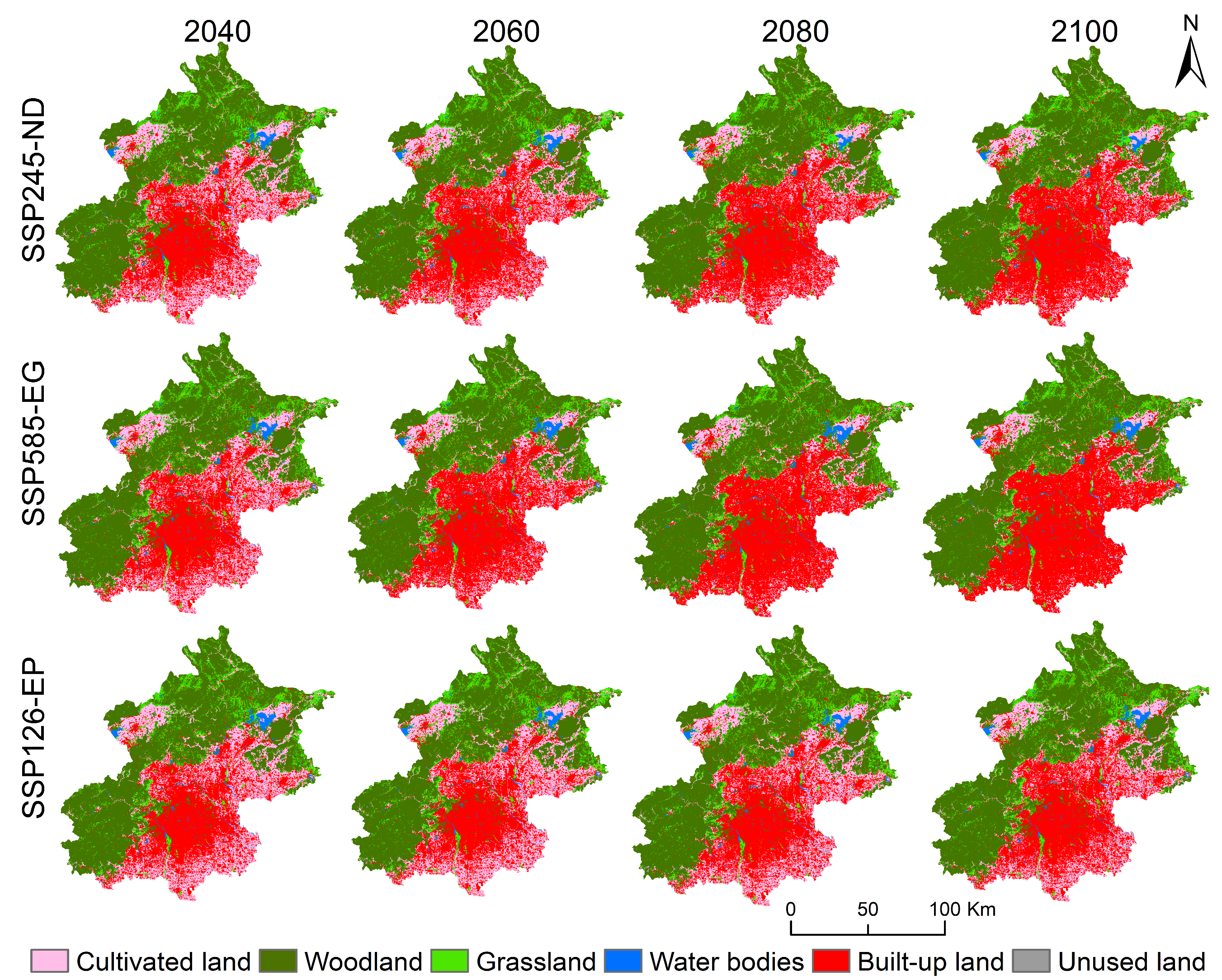
Based on the modified PLUS model simulation, the cultivated land in three scenarios showed a significant reduction trend, decreasing by 61%, 66.42%, and 45.5%, while the built-up land increased by 63.42%, 86.79%, and 38.9%. Only under the SSP126-EP scenario can both urban construction and the protection of cultivated land be possible.
(4)
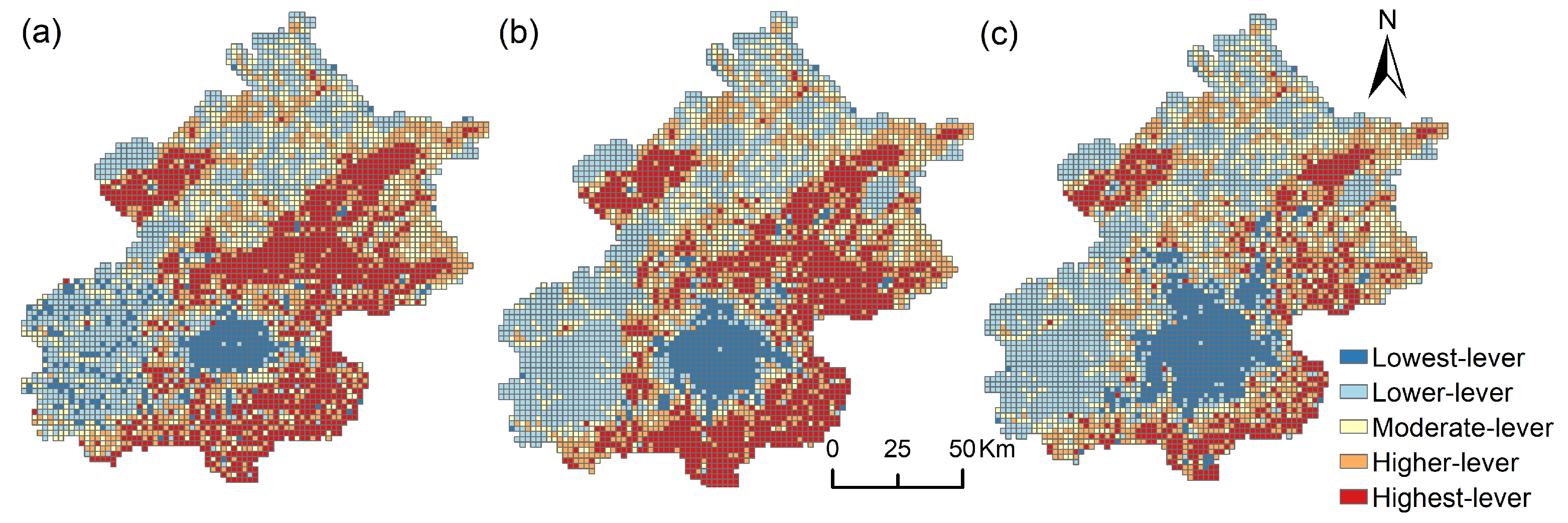
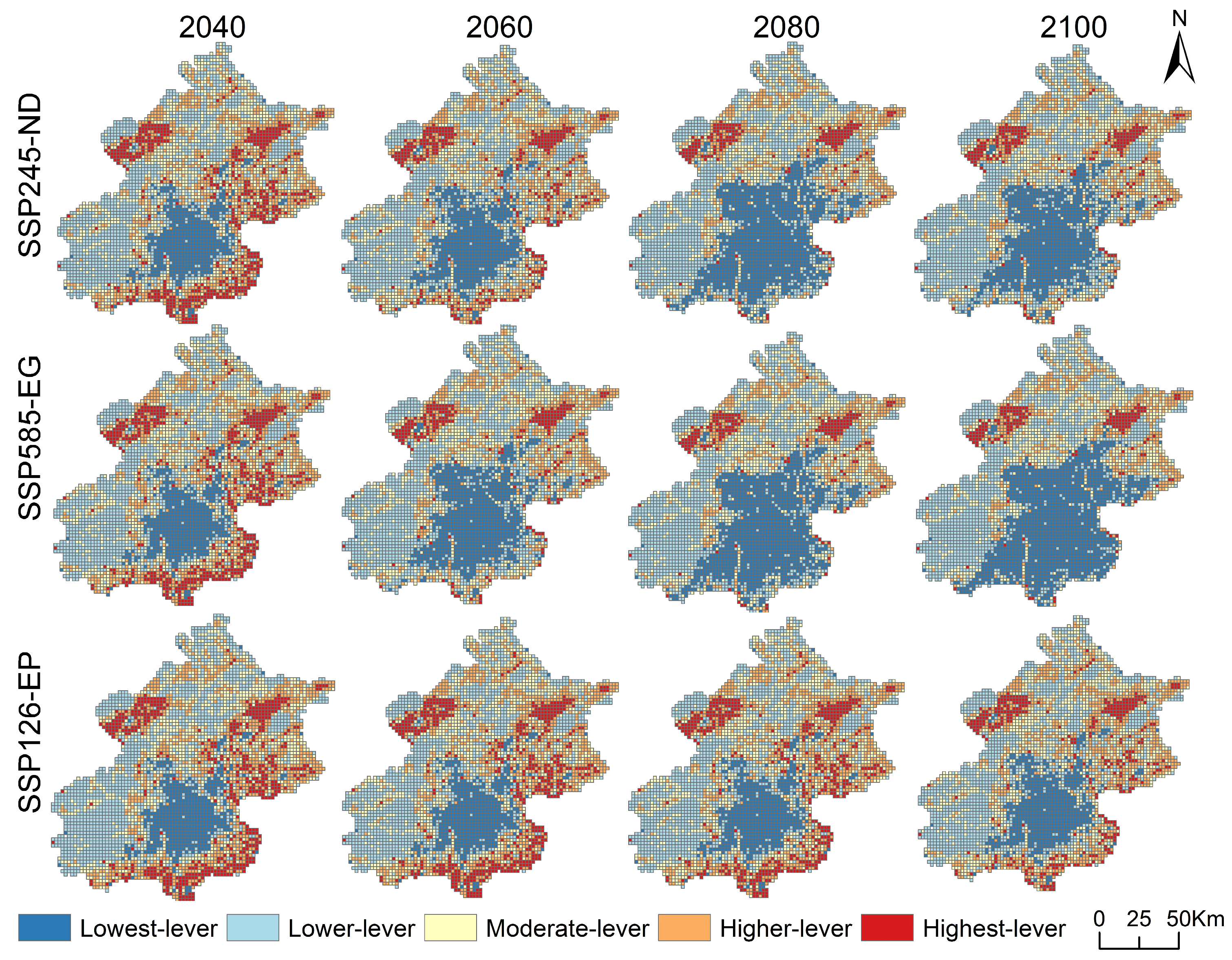
According to the LER index analysis, the LER in the past 20 years has been mainly lower, moderate, or higher, and the overall level of LER has shown a downward trend. However, under SSP245-ND and SSP585-EG, the overall ecological risk shows the lowest, lower, and moderate levels.
Future ecological risk assessments of urban landscapes will need to focus more on sustainable development and ecological conservation. Governments and policy makers can take measures to plan urban land use to minimize impacts on the natural environment, such as establishing ecological reserves, improving land use efficiency and improving urban planning to mitigate ecological risks.

Author Contributions

Conceptualization, Z.W. and D.Z.; methodology, Z.W., M.G. and H.Y.; software, M.G.; validation, D.Z., R.C. and H.Y.; writing—original draft preparation, M.G.; writing—review and editing, R.C., C.X. and H.Y.; visualization, M.G. and C.X.; supervision, D.Z.; project administration, Z.W.; funding acquisition, Z.W. and H.Y. All authors have read and agreed to the published version of the manuscript.

Funding

This research was funded by National Key R&D Program of China (grant number 2021YFC3200205), the Henan provincial key research and development program (grant number 221111321100) and the National Natural Science Foundation of China (grant number 41101561).

Data Availability Statement

Not applicable.

Acknowledgments

We thank LetPub (www.letpub.com, accessed on 13 July 2023) for its linguistic assistance during the preparation of this manuscript.

Conflicts of Interest

The authors declare no conflict of interest.

References

  1. Grimm, N.B.; Faeth, S.H.; Golubiewski, N.E.; Redman, C.L.; Wu, J.G.; Bai, X.M.; Briggs, J.M. Global change and the ecology of cities. Science 2008, 319, 756–760. [Google Scholar] [CrossRef] [PubMed]
  2. Tratalos, J.; Fuller, R.A.; Warren, P.H.; Davies, R.G.; Gaston, K.J. Urban form, biodiversity potential and ecosystem services. Landsc. Urban Plan. 2007, 83, 308–317. [Google Scholar] [CrossRef]
  3. Tsakiris, G.P.; Loucks, D.P. Adaptive Water Resources Management Under Climate Change: An Introduction. Water Resour. Manag. 2023, 37, 2221–2233. [Google Scholar] [CrossRef]
  4. Smeraldo, S.; Bosso, L.; Fraissinet, M.; Bordignon, L.; Brunelli, M.; Ancillotto, L.; Russo, D. Modelling risks posed by wind turbines and power lines to soaring birds: The black stork (Ciconia nigra) in Italy as a case study. Biodivers. Conserv. 2020, 29, 1959–1976. [Google Scholar] [CrossRef]
  5. Fraissinet, M.; Ancillotto, L.; Migliozzi, A.; Capasso, S.; Bosso, L.; Chamberlain, D.E.; Russo, D. Responses of avian assemblages to spatiotemporal landscape dynamics in urban ecosystems. Landsc. Ecol. 2023, 38, 293–305. [Google Scholar] [CrossRef]
  6. Vergel-Tovar, C.E. Understanding barriers and opportunities for promoting transit-oriented development with bus rapid transit in Bogot’a and Quito. Land. Use Policy 2023, 132, 106791. [Google Scholar] [CrossRef]
  7. Valbuena, D.; Verburg, P.H.; Bregt, A.K.; Ligtenberg, A. An agent-based approach to model land-use change at a regional scale. Landsc. Ecol. 2010, 25, 185–199. [Google Scholar] [CrossRef]
  8. Bai, T.; Fan, L.; Song, G.; Song, H.; Ru, X.; Wang, Y.; Zhang, H.; Min, R.; Wang, W. Effects of Land Use/Cover and Meteorological Changes on Regional Climate under Different SSP-RCP Scenarios: A Case Study in Zhengzhou, China. Remote Sens. 2023, 15, 2601. [Google Scholar] [CrossRef]
  9. Liang, X.; Liu, X.P.; Li, X.; Chen, Y.M.; Tian, H.; Yao, Y. Delineating multi-scenario urban growth boundaries with a CA-based FLUS model and morphological method. Landsc. Urban Plan. 2018, 177, 47–63. [Google Scholar] [CrossRef]
  10. He, C.Y.; Gao, B.; Huang, Q.X.; Ma, Q.; Dou, Y.Y. Environmental degradation in the urban areas of China: Evidence from multi-source remote sensing data. Remote Sens. Env. 2017, 193, 65–75. [Google Scholar] [CrossRef]
  11. Li, B.F.; Shi, X.; Lian, L.S.; Chen, Y.N.; Chen, Z.S.; Sun, X.Y. Quantifying the effects of climate variability, direct and indirect land use change, and human activities on runoff. J. Hydrol. 2020, 584, 124684. [Google Scholar] [CrossRef]
  12. Avashia, V.; Garg, A.; Dholakia, H. Understanding temperature related health risk in context of urban land use changes. Landsc. Urban Plan. 2021, 212, 104107. [Google Scholar] [CrossRef]
  13. Zhou, W.Q.; Qian, Y.G.; Li, X.M.; Li, W.F.; Han, L.J. Relationships between land cover and the surface urban heat island: Seasonal variability and effects of spatial and thematic resolution of land cover data on predicting land surface temperatures. Landsc. Ecol. 2014, 29, 153–167. [Google Scholar] [CrossRef]
  14. Mwambo, F.M.; Furst, C.; Nyarko, B.K.; Borgemeister, C.; Martius, C. Maize production and environmental costs: Resource evaluation and strategic land use planning for food security in northern Ghana by means of coupled emergy and data envelopment analysis. Land. Use Policy 2020, 95, 104490. [Google Scholar] [CrossRef]
  15. Mohammady, M. Land use change optimization using a new ensemble model in Ramian County, Iran. Env. Earth Sci. 2021, 80, 780. [Google Scholar] [CrossRef]
  16. Liu, X.P.; Liang, X.; Li, X.; Xu, X.C.; Ou, J.P.; Chen, Y.M.; Li, S.Y.; Wang, S.J.; Pei, F.S. A future land use simulation model (FLUS) for simulating multiple land use scenarios by coupling human and natural effects. Landsc. Urban Plan. 2017, 168, 94–116. [Google Scholar] [CrossRef]
  17. Gong, B.H.; Liu, Z.F. Assessing impacts of land use policies on environmental sustainability of oasis landscapes with scenario analysis: The case of northern China. Landsc. Ecol. 2021, 36, 1913–1932. [Google Scholar] [CrossRef]
  18. Liang, X.; Guan, Q.; Clarke, K.C.; Liu, S.; Wang, B.; Yao, Y. Understanding the drivers of sustainable land expansion using a patch-generating land use simulation (PLUS) model: A case study in Wuhan, China. Comput. Environ. Urban Syst. 2021, 85, 101569. [Google Scholar] [CrossRef]
  19. Buonincontri, M.P.; Bosso, L.; Smeraldo, S.; Chiusano, M.L.; Pasta, S.; Di Pasquale, G. Shedding light on the effects of climate and anthropogenic pressures on the disappearance of in the Italian lowlands: Evidence from archaeo-anthracology and spatial analyses. Sci. Total Environ. 2023, 877, 162893. [Google Scholar] [CrossRef]
  20. Wang, Y.S.; Yang, Z.H.; Yu, M.H.; Lin, R.Y.; Zhu, L.; Bai, F.P. Integrating Ecosystem Health and Services for Assessing Ecological Risk and its Response to Typical Land-Use Patterns in the Eco-fragile Region, North China. Env. Manag. 2023, 71, 867–884. [Google Scholar] [CrossRef]
  21. Li, J.L.; Pu, R.L.; Gong, H.B.; Luo, X.; Ye, M.Y.; Feng, B.X. Evolution Characteristics of Landscape Ecological Risk Patterns in Coastal Zones in Zhejiang Province, China. Sustainability 2017, 9, 584. [Google Scholar] [CrossRef]
  22. Liu, H.; Wang, H.; Liu, K. A review of ecological security assessment and relevant methods in China. Nat. Ecol. Conserv. 2005, 8, 34–37. [Google Scholar]
  23. Li, Z.-T.; Yuan, M.-J.; Hu, M.-M.; Wang, Y.-F.; Xia, B.-C. Evaluation of ecological security and influencing factors analysis based on robustness analysis and the BP-DEMALTE model: A case study of the Pearl River Delta urban agglomeration. Ecol. Indic. 2019, 101, 595–602. [Google Scholar] [CrossRef]
  24. Jin, X.; Jin, Y.X.; Mao, X.F. Ecological risk assessment of cities on the Tibetan Plateau based on land use/land cover changes—Case study of Delingha City. Ecol. Indic. 2019, 101, 185–191. [Google Scholar] [CrossRef]
  25. Feng, Y.; Liu, Y.; Liu, Y. Spatially explicit assessment of land ecological security with spatial variables and logistic regression modeling in Shanghai, China. Stoch. Environ. Res. Risk Assess. 2017, 31, 2235–2249. [Google Scholar] [CrossRef]
  26. Lin, Y.; Hu, X.; Zheng, X.; Hou, X.; Zhang, Z.; Zhou, X.; Qiu, R.; Lin, J. Spatial variations in the relationships between road network and landscape ecological risks in the highest forest coverage region of China. Ecol. Indic. 2019, 96, 392–403. [Google Scholar] [CrossRef]
  27. Wang, H.; Liu, X.; Zhao, C.; Chang, Y.; Liu, Y.; Zang, F. Spatial-temporal pattern analysis of landscape ecological risk assessment based on land use/land cover change in Baishuijiang National nature reserve in Gansu Province, China. Ecol. Indic. 2021, 124, 107454. [Google Scholar] [CrossRef]
  28. McEachran, Z.P.; Slesak, R.A.; Karwan, D.L. From skid trails to landscapes: Vegetation is the dominant factor influencing erosion after forest harvest in a low relief glaciated landscape. For. Ecol. Manag. 2018, 430, 299–311. [Google Scholar] [CrossRef]
  29. Mo, W.; Wang, Y.; Zhang, Y.; Zhuang, D. Impacts of road network expansion on landscape ecological risk in a megacity, China: A case study of Beijing. Sci. Total Env. 2017, 574, 1000–1011. [Google Scholar] [CrossRef]
  30. Xu, Q.; Guo, P.; Jin, M.; Qi, J. Multi-scenario landscape ecological risk assessment based on Markov–FLUS composite model. Geomat. Nat. Hazards Risk 2021, 12, 1449–1466. [Google Scholar] [CrossRef]
  31. Ghosh, S.; Chatterjee, N.D.; Dinda, S. Urban ecological security assessment and forecasting using integrated DEMATEL-ANP and CA-Markov models: A case study on Kolkata Metropolitan Area, India. Sustain. Cities Soc. 2021, 68, 102773. [Google Scholar] [CrossRef]
  32. Hou, Y.; Chen, Y.; Li, Z.; Li, Y.; Sun, F.; Zhang, S.; Wang, C.; Feng, M. Land Use Dynamic Changes in an Arid Inland River Basin Based on Multi-Scenario Simulation. Remote Sens. 2022, 14, 2797. [Google Scholar] [CrossRef]
  33. Li, P.; Chen, J.; Li, Y.; Wu, W. Using the InVEST-PLUS Model to Predict and Analyze the Pattern of Ecosystem Carbon storage in Liaoning Province, China. Remote Sens. 2023, 15, 4050. [Google Scholar] [CrossRef]
  34. Zhang, S.; Zhong, Q.; Cheng, D.; Xu, C.; Chang, Y.; Lin, Y.; Li, B. Landscape ecological risk projection based on the PLUS model under the localized shared socioeconomic pathways in the Fujian Delta region. Ecol. Indic. 2022, 136, 108642. [Google Scholar] [CrossRef]
  35. Qiao, K.; Zhu, W.Q.; Hu, D.Y.; Hao, M.; Chen, S.S.; Cao, S.S. Examining the distribution and dynamics of impervious surface in different function zones in Beijing. J. Geogr. Sci. 2018, 28, 669–684. [Google Scholar] [CrossRef]
  36. Xu, X. China Annual Spatial Interpolation Dataset of Meteorological Elements. 2022. Available online: https://www.resdc.cn/DOI/doi.aspx?DOIid=96 (accessed on 1 September 2022). [CrossRef]
  37. Xu, X. China GDP Spatial Distribution Kilometer Grid Dataset. Data Regist. Publ. Syst. Resour. Environ. Sci. DataCent. Chin. Acad. Sci. 2017, 10, 2017121102. [Google Scholar] [CrossRef]
  38. Wu, J.; Luo, J.; Zhang, H.; Qin, S.; Yu, M. Projections of land use change and habitat quality assessment by coupling climate change and development patterns. Sci. Total Environ. 2022, 847, 157491. [Google Scholar] [CrossRef]
  39. Morris, M.D. Factorial Sampling Plans for Preliminary Computational Experiments. Technometrics 1991, 33, 161–174. [Google Scholar] [CrossRef]
  40. Francos, A.; Elorza, F.J.; Bouraoui, F.; Bidoglio, G.; Galbiati, L. Sensitivity analysis of distributed environmental simulation models: Understanding the model behaviour in hydrological studies at the catchment scale. Reliab. Eng. Syst. Safe 2003, 79, 205–218. [Google Scholar] [CrossRef]
  41. Wang, Y.; Li, X.; Zhang, Q.; Li, J.; Zhou, X. Projections of future land use changes: Multiple scenarios-based impacts analysis on ecosystem services for Wuhan city, China. Ecol. Indic. 2018, 94, 430–445. [Google Scholar] [CrossRef]
  42. Pontius, R.G.; Peethambaram, S.; Castella, J.C. Comparison of Three Maps at Multiple Resolutions: A Case Study of Land Change Simulation in Cho Don District, Vietnam. Ann. Assoc. Am. Geogr. 2011, 101, 45–62. [Google Scholar] [CrossRef]
  43. Pontius, R.G.; Boersma, W.; Castella, J.C.; Clarke, K.; de Nijs, T.; Dietzel, C.; Duan, Z.; Fotsing, E.; Goldstein, N.; Kok, K.; et al. Comparing the input, output, and validation maps for several models of land change. Ann. Reg. Sci. 2008, 42, 11–37. [Google Scholar] [CrossRef]
  44. Chen, J.; Chen, J.; Liao, A.; Cao, X.; Chen, L.; Chen, X.; He, C.; Han, G.; Peng, S.; Lu, M.; et al. Global land cover mapping at 30 m resolution: A POK-based operational approach. Isprs J. Photogramm. 2015, 103, 7–27. [Google Scholar] [CrossRef]
  45. Brovelli, M.; Molinari, M.; Hussein, E.; Chen, J.; Li, R. The First Comprehensive Accuracy Assessment of GlobeLand30 at a National Level: Methodology and Results. Remote Sens. 2015, 7, 4191–4212. [Google Scholar] [CrossRef]
  46. Xu, H. Modification of normalised difference water index (NDWI) to enhance open water features in remotely sensed imagery. Int. J. Remote Sens. 2007, 27, 3025–3033. [Google Scholar] [CrossRef]
  47. Balcik, F.B. Determining the impact of urban components on land surface temperature of Istanbul by using remote sensing indices. Env. Monit. Assess. 2014, 186, 859–872. [Google Scholar] [CrossRef]
  48. Rahnama, M.R. Forecasting land-use changes in Mashhad Metropolitan area using Cellular Automata and Markov chain model for 2016–2030. Sustain. Cities Soc. 2021, 64, 102548. [Google Scholar] [CrossRef]
  49. O’Neill, B.C.; Tebaldi, C.; van Vuuren, D.P.; Eyring, V.; Friedlingstein, P.; Hurtt, G.; Knutti, R.; Kriegler, E.; Lamarque, J.F.; Lowe, J.; et al. The Scenario Model Intercomparison Project (ScenarioMIP) for CMIP6. Geosci. Model. Dev. 2016, 9, 3461–3482. [Google Scholar] [CrossRef]
  50. Liao, W.; Liu, X.; Xu, X.; Chen, G.; Liang, X.; Zhang, H.; Li, X. Projections of land use changes under the plant functional type classification in different SSP-RCP scenarios in China. Sci. Bull. 2020, 65, 1935–1947. [Google Scholar] [CrossRef]
  51. Tian, L.; Tao, Y.; Fu, W.; Li, T.; Ren, F.; Li, M. Dynamic Simulation of Land Use/Cover Change and Assessment of Forest Ecosystem Carbon Storage under Climate Change Scenarios in Guangdong Province, China. Remote Sens. 2022, 14, 2330. [Google Scholar] [CrossRef]
  52. Tian, P.; Cao, L.; Li, J.; Pu, R.; Gong, H.; Li, C. Landscape Characteristics and Ecological Risk Assessment Based on Multi-Scenario Simulations: A Case Study of Yancheng Coastal Wetland, China. Sustainability 2020, 13, 149. [Google Scholar] [CrossRef]
  53. Tian, P.; Li, J.; Gong, H.; Pu, R.; Cao, L.; Shao, S.; Shi, Z.; Feng, X.; Wang, L.; Liu, R. Research on Land Use Changes and Ecological Risk Assessment in Yongjiang River Basin in Zhejiang Province, China. Sustainability 2019, 11, 2817. [Google Scholar] [CrossRef]
  54. Yang, Y.; Yang, X.; Li, E.; Huang, W. Transitions in land use and cover and their dynamic mechanisms in the Haihe River Basin, China. Env. Earth Sci. 2021, 80, 50. [Google Scholar] [CrossRef]
  55. Zhang, W.; Chang, W.J.; Zhu, Z.C.; Hui, Z. Landscape ecological risk assessment of Chinese coastal cities based on land use change. Appl. Geogr. 2020, 117, 102174. [Google Scholar] [CrossRef]
  56. Zhou, Y.; Li, X.; Liu, Y. Land use change and driving factors in rural China during the period 1995–2015. Land Use Policy 2020, 99, 105048. [Google Scholar] [CrossRef]
  57. Homewood, K.; Lambin, E.F.; Coast, E.; Kariuki, A.; Kikula, I.; Kivelia, J.; Said, M.; Serneels, S.; Thompson, M. Long-term changes in Serengeti-Mara wildebeest and land cover: Pastoralism, population, or policies? Proc. Natl. Acad. Sci. USA 2001, 98, 12544–12549. [Google Scholar] [CrossRef]
  58. He, C. Modelling scenarios of land use change in northern China in the next 50 years. J. Geogr. Sci. 2005, 15, 177. [Google Scholar] [CrossRef]
  59. Zheng, Q.M.; Weng, Q.H.; Wang, K. Characterizing urban land changes of 30 global megacities using nighttime light time series stacks. Isprs J. Photogramm. 2021, 173, 10–23. [Google Scholar] [CrossRef]
  60. Verburg, P.H.; Eickhout, B.; van Meijl, H. A multi-scale, multi-model approach for analyzing the future dynamics of European land use. Ann. Reg. Sci. 2007, 42, 57–77. [Google Scholar] [CrossRef]
  61. Jia, S.; Yang, Y. Spatiotemporal and Driving Factors of Land-Cover Change in the Heilongjiang (Amur) River Basin. Remote Sens. 2023, 15, 3730. [Google Scholar] [CrossRef]
  62. Gao, L.; Tao, F.; Liu, R.; Wang, Z.; Leng, H.; Zhou, T. Multi-scenario simulation and ecological risk analysis of land use based on the PLUS model: A case study of Nanjing. Sustain. Cities Soc. 2022, 85, 104055. [Google Scholar] [CrossRef]
  63. Turner, B.L.; Lambin, E.F.; Reenberg, A. The emergence of land change science for global environmental change and sustainability. Proc. Natl. Acad. Sci. USA 2007, 104, 20666–20671. [Google Scholar] [CrossRef] [PubMed]
  64. Chen, Z.Z.; Huang, M.; Zhu, D.Y.; Altan, O. Integrating Remote Sensing and a Markov-FLUS Model to Simulate Future Land Use Changes in Hokkaido, Japan. Remote Sens. 2021, 13, 2621. [Google Scholar] [CrossRef]
  65. Saltelli, A.; Annoni, P.; Azzini, I.; Campolongo, F.; Ratto, M.; Tarantola, S. Variance based sensitivity analysis of model output. Design and estimator for the total sensitivity index. Comput. Phys. Commun. 2010, 181, 259–270. [Google Scholar] [CrossRef]
  66. Ratto, M.; Tarantola, S.; Saltelli, A. Sensitivity analysis in model calibration: GSA-GLUE approach. Comput. Phys. Commun. 2001, 136, 212–224. [Google Scholar] [CrossRef]
  67. Ju, H.; Niu, C.; Zhang, S.; Jiang, W.; Zhang, Z.; Zhang, X.; Yang, Z.; Cui, Y. Spatiotemporal patterns and modifiable areal unit problems of the landscape ecological risk in coastal areas: A case study of the Shandong Peninsula, China. J. Clean. Prod. 2021, 310, 127522. [Google Scholar] [CrossRef]
  68. Xu, J.; Kang, J. Comparison of Ecological Risk among Different Urban Patterns Based on System Dynamics Modeling of Urban Development. J. Urban Plan. Dev. 2017, 143, 04016034. [Google Scholar] [CrossRef]
  69. Tang, L.; Wang, L.; Li, Q.; Zhao, J. A framework designation for the assessment of urban ecological risks. Int. J. Sustain. Dev. World Ecol. 2018, 25, 387–395. [Google Scholar] [CrossRef]
Figure 1. Study area. Geographic location of Beijing, the division of the city and its four functional districts.
Remotesensing 15 05186 g001
Figure 2. Flowchart of land use simulation based on the PLUS Model and landscape ecological risk assessment in Beijing.
Remotesensing 15 05186 g002
Figure 3. Land use data before and after NDISI calibration in 2000, 2010, and 2020.
Remotesensing 15 05186 g003
Figure 4. Presentation of land use data by functional areas, 2000–2020: analyses based on the calibrated NDISI.
Remotesensing 15 05186 g004
Figure 5. Selection of the indicators with the best accuracy by combining the parameter ranges determined by the sensitivity analyses.
Remotesensing 15 05186 g005
Figure 6. Comparison of spatial distribution of real data and simulation results of land use pattern in 2010 and 2020 ((a,c) are calibrated GlobalLand30 data; (b,d) are the results of the PLUS simulation).
Remotesensing 15 05186 g006
Figure 7. Analysis of the contribution of various drivers to each land use type (“D-” indicates the closest distance to the road).
Remotesensing 15 05186 g007
Figure 8. Proportion of area of various land use types in Beijing in 2040, 2060, 2080 and 2100 predicted by Markov.
Remotesensing 15 05186 g008
Figure 9. Simulation of land use in Beijing under different scenarios based on the PLUS model.
Remotesensing 15 05186 g009
Figure 10. Spatial distribution of LER in 2000, 2010, and 2020. ((ac) indicate 2000, 2010, and 2020, respectively).
Remotesensing 15 05186 g010
Figure 11. Spatial distribution of LER in future under different scenarios.
Remotesensing 15 05186 g011
Table 1. Details of all data types, including land use, climate environment, socio-economics and constraints.
TypeDataResolutionMeaningData Source
Land useLand use classification data in 2000, 2010 and 202030 m1 Cultivated land; 2 woodland; 3 grassland; 4 water bodies; 5 built-up land; 6 unused land30 m Global land cover data
http://www.GlobalLandcover.com/, accessed on 1 September 2022
Limiting factorFixed rivers, reservoirs, lakes, and slopes greater than 25° in the city30 mThe area is off limits to developmentGlobeLand30 and ASTER GDEM v3
Climate and environmental dataMean annual precipitation (mm)30 mThe average annual precipitation at the location corresponding to the pixelResources and Environmental Science and Data Center, CAS [36]
http://www.resdc.cn/, accessed on 1 September 2022
Mean annual temperature (°C)30 mThe average annual temperature at the location corresponding to the pixel
Elevation (m)30 mTopographic elevation conditionASTER GDEM v3
https://earthdata.nasa.gov/, accessed on 1 September 2022
Slope (°)30 mTopographic slope condition
Social economy dataGDP (10,000 yuan/km2)30 mThe GDP value of each pixel locationResources and Environmental Science and Data Center, CAS [37]
http://www.resdc.cn/, accessed on 1 September 2022
The number of people/persons30 mThe number of people in each pixel’s locationWorldPop
https://www.worldpop.org/, accessed on 1 September 2022
The distance to the main road (m), the primary road (m), the secondary road (m), the tertiary road (m), the motorway road (m) and the rail road (m)30 mThe nearest Euclidean distance from the pixel geometric center to the roadOpenStreetMap
https://www.openstreetmap.org/, accessed on 1 September 2022
Table 2. Comparison of overall accuracy, kappa coefficient and F o M value before and after land use data calibration.
TypeYearOverallKappa F o M
GLC3020100.8140.7820.153
20200.8250.7510.179
GLC30-NDISI20100.860.7970.155
20200.8620.80.18
Table 3. Comparison of overall accuracy, kappa coefficient and F o M value before and after Morris parameter calibration.
TypeYearOverallKappa F o M
Traditional20100.860.7970.155
20200.8620.80.18
After correction20100.8670.8260.224
20200.8760.8140.21
Table 4. Area statistics for the five standard risk levels under multiple scenarios.
Category20202040206020802100
EGEPNDEGEPNDEGEPNDEGEPND
Lowest11.4711.7711.4711.5819.9611.6314.9525.8212.3425.8730.4914.1521.41
Lower31.9830.0631.9430.2234.8229.6233.2634.7829.9734.8033.4231.0936.22
Moderate23.2124.4022.9924.2024.0824.3824.8921.9325.1121.8220.2625.6423.28
Higher20.7621.3620.8121.2215.7321.5019.3712.9121.2912.9611.6820.6714.17
Highest12.5712.4112.8012.775.4012.877.534.5611.294.564.148.454.92
Disclaimer/Publisher’s Note: The statements, opinions and data contained in all publications are solely those of the individual author(s) and contributor(s) and not of MDPI and/or the editor(s). MDPI and/or the editor(s) disclaim responsibility for any injury to people or property resulting from any ideas, methods, instructions or products referred to in the content.

