Article

Impervious Surface Area Patterns and Their Response to Land Surface Temperature Mechanism in Urban–Rural Regions of Qingdao, China

1
Key Laboratory of Terrestrial Ecological Remediation in Jining City, School of Geography and Tourism, Qufu Normal University, Rizhao 276826, China
2
Key Laboratory of Land Surface Pattern and Simulation, Institute of Geographic Sciences and Natural Resources Research, Chinese Academy of Sciences, Beijing 100101, China
*
Author to whom correspondence should be addressed.
Remote Sens. 2023, 15(17), 4265; https://doi.org/10.3390/rs15174265
Submission received: 7 July 2023 / Revised: 13 August 2023 / Accepted: 28 August 2023 / Published: 30 August 2023

Abstract

:
The expansion of impervious surface area (ISA) in megacities of China often leads to land surface temperature (LST) aggregation effects, which affect living environments by impacting thermal comfort levels, thus becoming an issue of public concern. However, from an urban–rural synchronous comparison perspective, the study of LST responses to ISA changes is still lacking in the central coastal megalopolises of China. To solve this issue, a collaborative methodology of artificial digitization—fully constrained least squares mixed pixel decomposition—split-window algorithm—PCACA model was established for Qingdao using land use dataset and remote sensing images. The conclusions are below. Long time series of land use monitoring indicated that the expansion ratios of urban and rural areas were 131.29% and 43.42% in the past 50 years (i.e., from 1970 to 2020). Within urban and rural areas, a synchronous ISA increase was observed, with ratios of +9.14% (140.55 km2) and +7.94% (28.04 km2), respectively. Higher ratios and area changes were found in the urban regions, and a similar ISA change pattern in both urban and rural regions was captured by the ISA horizontal epitaxial expansion and vertical density enhancement. Further, the horizontal gradient effect displayed that the mean LSTs were 28.75 °C, 29.77 °C and 31.91 °C in the urban areas and 28.73 °C, 29.66 °C and 31.65 °C in the rural areas in low-, medium-, and high-density ISAs. The vertical density effect showed that the LST change was 1.02 °C and 2.14 °C in the urban areas but 0.93 °C and 1.99 °C in the rural areas during the ISA-density transition from low- to medium- and from medium- to high-density, respectively. Potential surface thermal indicators were assessed, and the urban regions displayed higher sensible heat flux (280.13 W/m2) compared to the rural regions (i.e., 274.76 W/m2). The mechanism effect of the ISA changes on LST in the urban and rural regions was revealed. These findings form a new comparative perspective of the urban–rural synchronous change in the central coastal megalopolis of China and can provide a practical reference for relevant studies.

Graphical Abstract

1. Introduction

Monitoring the impervious surface area patterns and exploring their response to land surface temperature is always a hot topic in the academic field. Since the 21st century, impervious surface area (ISA) has displayed a large-scale increasing trend throughout China [1] under the driving forces of rapid urban–rural expansion [2,3], industrial development [4], population growth [5] and the continuous improvement of residents’ living standards [6]. ISAs are areas where rainwater cannot penetrate and include roads, city squares, and building roofs, etc. [7,8]. These areas clearly impact the distribution of land surface radiation and the energy balance [9], which directly influence comfortable living environments and receive widespread attention worldwide. Thus, ISA has become an essential indicator for land use transformation from natural land coverage to artificial surfaces at different spatial and temporal scales [10]. In particular, the ISA causes direct or indirect environmental influences on local and regional surface runoff, water quality [11], energy balance, and biodiversity [12,13]. Meanwhile, an obvious effect of the expansion pattern of ISA is the increasing land surface temperature (LST) effect due to the inherent attributes of impervious surface area such as low albedo, large heat capacity, and weak evaporation and transpiration [14,15]. LST plays an important role in the exchange of matter and energy between the low boundary of the atmosphere [16], local ocean current circulation, and climate change [17,18,19] and it especially impacts the near-surface ecological environment pattern, hydropower energy consumption, and residents’ personal health [20,21,22,23]. Therefore, the clarification of the spatiotemporal change in ISA and its LST response characteristics is needed to reasonably lay out regional living space, production space, and ecological space to improve ecological service functions and the quality of human living environments.
With the development of high-resolution images and the increasing maturity of remote sensing processing technology, the mapping of ISAs from remote sensing images has received more attention and has become a mainstream method [24,25]. Generally, high-resolution remote sensing images can achieve high spatial resolution mapping of ISAs, but they are not widely popularized due to the difficulty of obtaining data sources, the discontinuity of time, and the expense of purchasing images and hiring professionals [7]. Automatic classification has typically had difficulty in achieving high-accuracy results from high-resolution remote sensing images because the same land-type object may display different spectral characteristics and the same spectral characteristics may contain different land-type objects [4,6]. Medium-resolution remote sensing images, such as those from the Landsat program, which feature suitable spectral properties, free download, and good accuracy, are widely used for ISA mapping [6]. For the spatial mapping methodology of ISA, scholars have conducted extensive discussions [26,27]. The vegetation-impervious surface-soil (V-I-S) model was proposed first [28,29]; it stated that the land surface was composed of four land-cover components, including vegetation, bare soil, ISA, and water bodies. This linear decomposition approach was predicted to resolve Landsat image resolution issues, and a method was developed to assign image pixels to different land type components (i.e., subpixel classification) [12,28]. Then, a combined method that used the linear spectral mixture analysis model (LSMA) and the V-I-S model was established to obtain the ISA in the Columbus, Ohio region of the United States [12,30]. Subsequent studies also confirmed that the combination of LSMA and V-I-S models easily obtained ISA at local, regional, and even global scales [31]. This method became widely used for spatiotemporal mapping and monitoring the dynamic change in the ISA.
To study the LST and energy mechanisms, domestic and foreign scholars have conducted extensive research on thermal infrared remote sensing data retrieved from Landsat images. The single window algorithm model, as a local and regional surface temperature retrieval technique for Landsat Thematic Mapper (TM) images, has been widely used with high accuracy [32]. Subsequently, to obtain a more accurate LST spatial pattern, the single window model was upgraded to the split algorithm model method in response to the emergence of Landsat 8/9 Operational Land Imager (OLI) satellite imagery, which had two thermal infrared bands [33,34]. Furthermore, the pixel component arranging and component algorithm (PCACA) model can investigate the mechanisms of temperature and energy changes on the land surface [35]. Through the PCACA model, the spatial coefficients of sensible heat flux and latent heat flux were obtained; these were input into the surface radiation energy balance model to generate mechanism indicators such as latent heat flux, sensible heat flux, soil heat flux, and net radiation [35]. This approach provided a basis for the exploration of LST change and its energy mechanisms.
Spatiotemporal changes in ISA alter the land temperature and energy level, affecting the comfort level of the living environment and thus creating an issue of public concern. Although relevant studies have been conducted in some regions, the studies on the comparison of the synchronous ISA change in the urban–rural areas and their response characteristics to LST mechanisms are still lacking in the central coastal megalopolises of China. This situation limits the exploration of the relationship between regional land use changes and the thermal comfort level of living environments. To address this issue, we need to create urban and rural boundaries, retrieve ISA density data, explore the temperature effect of different ISA densities, and reveal mechanisms. Therefore, the aims of this study are to (1) provide long time series of urban–rural land change monitoring from 1970 to 2020 to understand the historical process and heterogeneity of urban–rural regions in the coastal areas of central China; (2) conduct land-cover mapping of the ISA components and compare their changes from urban–rural synchronous change perspective and (3) characterize the spatiotemporal heterogeneity of LST and further investigate temperature responses under different densities in urban and rural ISAs. In addition, the mechanism by which impervious surface areas affect temperature is also revealed. We hope that the analysis of land use, ISA, LST, and energy mechanisms from a comparative perspective of the urban–rural synchronous change in the central coastal areas of China in this study can provide a practical reference for related studies.

2. Materials and Methods
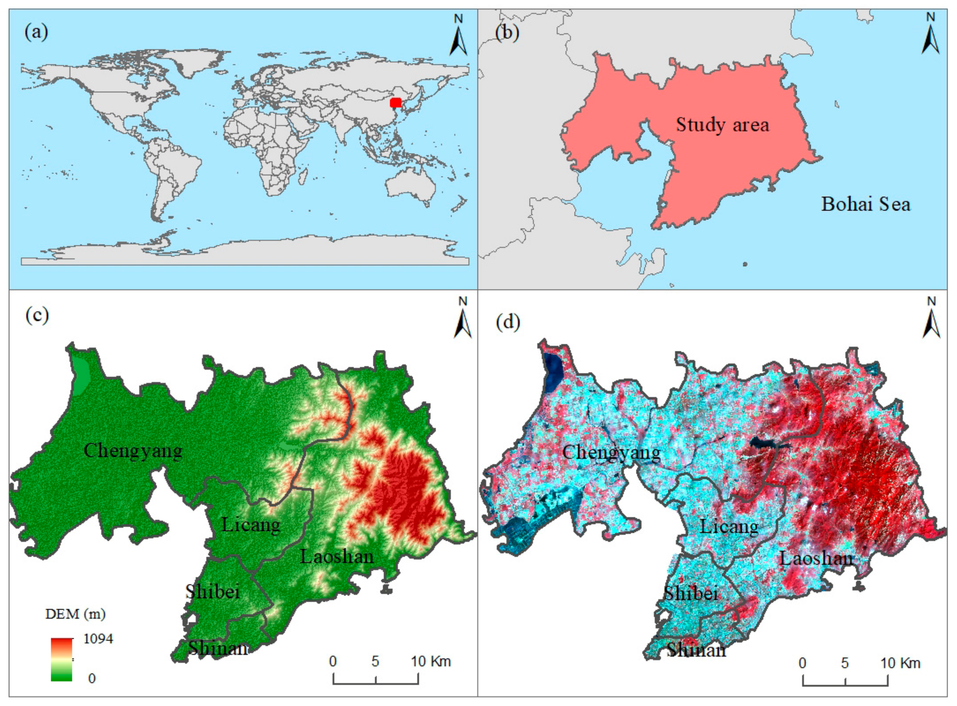
2.1. Study Area

Qingdao is in the coastal area of central China, with a longitude ranging from 119°30′ to 121°00′E and a latitude ranging from 35°35′ to 37°09′N (Figure 1a,b). Qingdao has played an important role nationally in the development of the modern marine industry; it is an international shipping hub in northeast Asia, and a leading region for economic and trade cooperation between China, Japan, and South Korea. At the end of 2022, the resident population of Qingdao was 10.34 million, with an urbanization rate of 77.32%. The gross domestic product was 1492.075 billion yuan, and the structure of the primary, secondary, and tertiary industries was 3.2%, 34.8%, and 62.0%, respectively. This region has a northern temperate monsoon climate. The digital elevation model (DEM) shows that Qingdao is high in the east and low in the west (Figure 1c). The high terrain regions in the east are mainly mountainous, while residential regions are concentrated in the west, which can be recognized in the remote sensing images shown in Figure 1d. There are 33 large rivers with a drainage area of over 100 km2, which are divided into three major water systems, including the Dagu River, Beijiaolai River and coastal areas. The soil mainly consists of five soil types: brown soil, sandy ginger black soil, tidal soil, brown soil, and saline soil. This study focuses on the central city of Qingdao, which includes the Shinan, Shibei, Licang, Laoshan and Chengyang Districts.

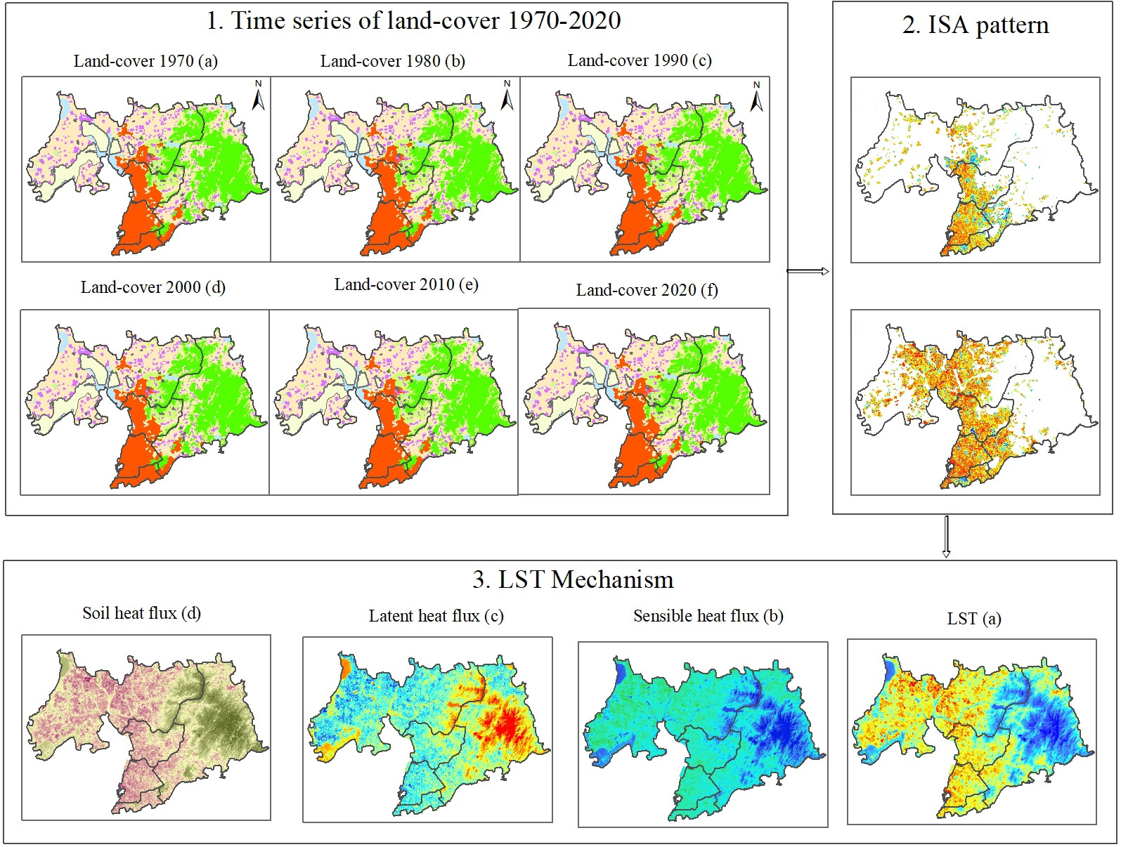
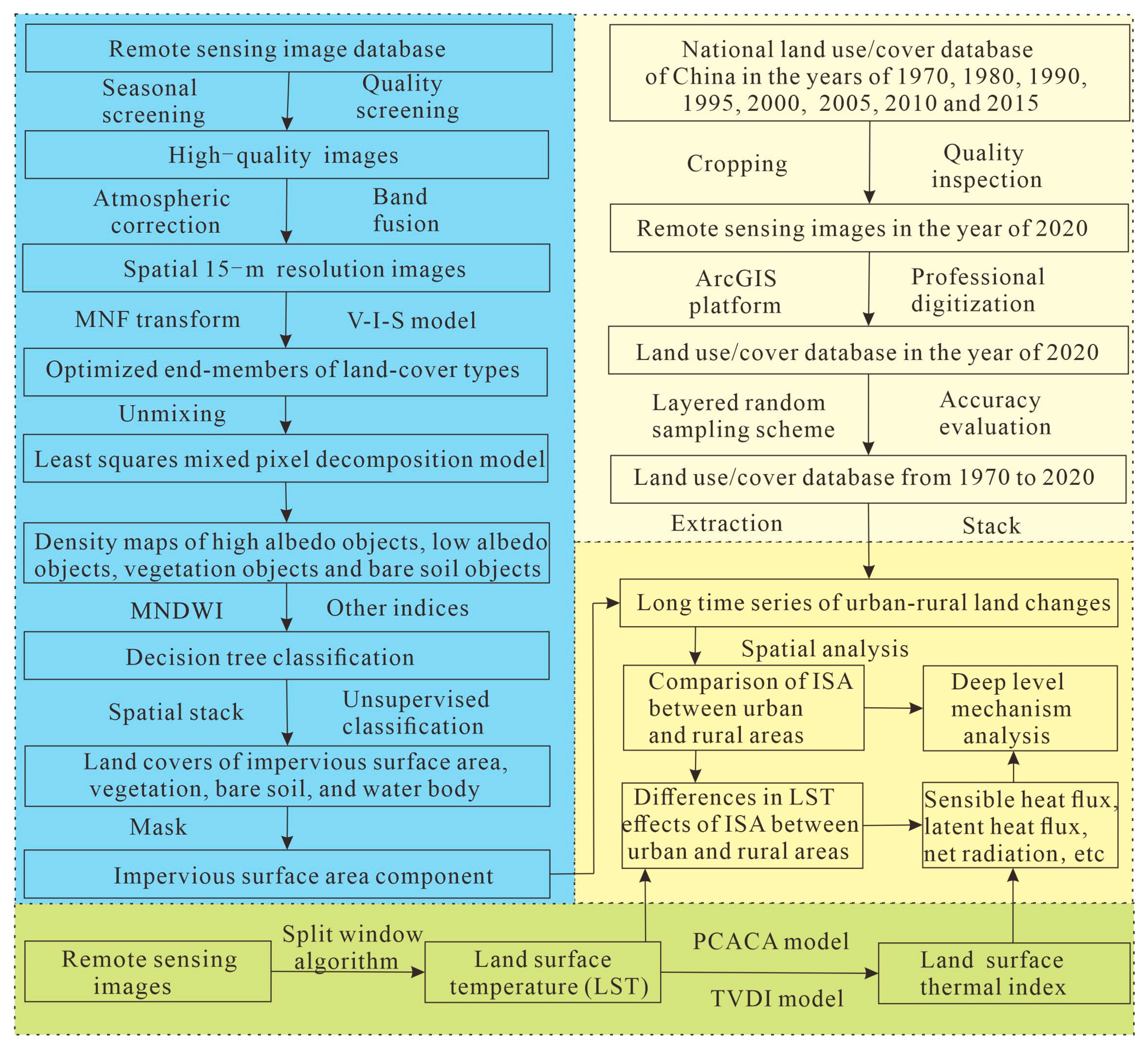
2.2. Flowchart of This Study

The technical process of this study was shown in the following Figure 2. Firstly, this study conducted the long time series of urban–rural change monitoring and its regional differences through 50 years from 1970 to 2020, to understand the historical process and heterogeneity of urban–rural regions in the coastal areas of China; to obtain the latest land use mapping, the human–computer interactive interpretation method of remotely sensed information to interpret the Landsat digital images was applied to establish new land use maps in 2020 using the national land use/cover database of China in 2015 and remote sensing images. After producing the land use data in 2020, the accuracy evaluation was conducted using the method of a layered random sampling scheme. The obtained land use accuracies were both over 92%. The long time series of spatiotemporal features of urban–rural differences were compared. Secondly, we conducted the land-cover mapping of urban–rural ISA components and compared the changes in their differences. For generating the ISA within the urban and rural areas, the Vegetation—Impervious surface—Soil (V-I-S) model was used to obtain the optimal endmembers of the different types of land covers from remote sensing images, which were input with the least squares mixed pixel decomposition model to generate the densities of high albedo objects, low albedo objects, vegetation objects and bare soil objects. These four densities, as well as other indexes, were used to generate the land covers of impervious surface area, vegetation, bare soil, and water bodies using a decision tree classifier. The remaining few unclassified areas were classified through unsupervised classification and manual recognition. The cover of ISA types was then extracted and superimposed to the densities of high albedo objects and low albedo objects to generate the ISA component data. Using the urban–rural boundaries, the ISA in urban–rural areas were clipped and analyzed. Thirdly, a split window algorithm was used to generate a surface temperature pattern. The surface radiation energy balance model, PCACA model and TVDI model were then used to obtain variously spatialized thermal comfort indicators, including the sensible heat flux, latent heat flux, etc. Then, the urban–rural temperature effect of ISA was revealed as well as its surface thermal attribute mechanism.

2.3. Production of Land-Use Data in 2020 and Extraction of Urban–Rural Boundaries from 1970 to 2020

2.3.1. Land Use Data Acquisition

Land-cover data of the study area in 1970, 1980, 1990, 1995, 2000, 2005, 2010 and 2015 were sourced from the land-use/cover change (LUCC) dataset of the national resources and environment remote sensing spatiotemporal information platform of the Chinese Academy of Sciences. These data had a comprehensive evaluation accuracy of over 90.00% for first-class land type. The data format was a vector polygon file. Land data from 2015 were used to produce the land cover of the study area in 2020.

2.3.2. Land Classification System Description of Urban and Rural Areas

The land-use classification system in this study was consistent with the LUCC dataset of the Chinese Academy of Sciences [36], including six first-level land categories of cropland, woodland, grassland, construction land, water land, and unused land, accompanied by land type codes of 10, 20, 30, 40, 50 and 60, respectively [37]. These six first-level categories were further divided into 25 secondary categories. One advantage of this land data classification system was that the construction land (i.e., code 50) was divided into three categories of urban land (i.e., code 51), rural land (i.e., code 52), and independent industrial and mining land (i.e., code 53) [36,37], compared to most other land data classification systems that set construction land as only one land category layer [38,39]. In the land data classification system of the Chinese Academy of Sciences data, urban land refers to built-up areas in large, medium, and small cities, as well as counties, and rural land refers to rural settlements that are independent of urban land [37]. The urban and rural land boundaries of this dataset achieved good results in many studies on land use and land use change monitoring [36,40]. In this study, urban and rural lands were used to analyze spatiotemporal changes and further served as masks for urban and rural ISAs.

2.3.3. Remote Sensing Image Download and Data Preprocessing

To produce the land data for 2020, the Landsat images with good quality were filtered from the USGS official website (http://glovis.usgs.gov/, accessed on 11 March 2022) to avoid interference from bad pixels, stripes, clouds, and rain on the images. The time of the images was set as summer (i.e., from July to September), which was conducive to distinguishing different land-cover types in the Landsat images. The downloaded high-quality images were input into the ENVI platform for spatial registration and band fusion purposes. Gram–Schmidt pan sharpening algorithms fused the Landsat multispectral band and panchromatic band, increasing the image resolution from 30 m to 15 m resolution. The image adopted a false color synthesis method, as false color is commonly used for land change monitoring and interpretation.

2.3.4. Digital Visualization and Acquisition of Urban–Rural Dynamic Land

The human–computer interactive interpretation method of remotely sensed information to interpret the Landsat digital images was applied to establish a new land use map in 2020, using the land use/cover data in 2015 and Landsat images in 2020. The projection and coordinates of land use data and remote sensing images were first set the same to ensure spatial position matching. Then, taking the remote sensing images in the year 2020 as the first layer data on the ArcGIS platform, we superimposed the land-use vector data in the year 2015 onto these images, and thus the land-use data was as the second layer data. An attribute table named land 2020 was created in land use data for storing the required 2020 land cover type code. After that, the human–computer interactive interpretation technology was used to depict the land use in the year 2020, using the professional knowledge of identifying color, brightness, and texture features for cropland, forest land, grassland, water land, urban land, rural land, and other lands in the remote sensing images. When a land cover type was identified on remote sensing images, A numerical code was assigned to this land cover and was filled in the attribute table (i.e., land 2020). If the land cover type was difficult to identify, online historical Google images and high-resolution satellites were used as auxiliary reference data to identify this land type. We repeated this process until all regions were interpreted through human-computer interaction. Then, the attribute table (i.e., land 2020) recorded the codes for all 2020 land use types.
To ensure the quality of the land use data, we conducted data checks through different persons. Dynamic land-use patches from 2015 to 2020 were first extracted through the attribute Table 2015 and the attribute Table 2020. Then, the different professionals rechecked whether the land code was correct or not using the Landsat images on the ArcGIS platform. After that, a data quality accuracy evaluation was performed. The 2-m Google Image in the study area was used as an accuracy evaluation image data source and was downloaded through a paid and professional software platform (i.e., Bitmap). A hierarchical random sampling method was used to obtain the confusion matrix. In this confusion matrix, the producers’ accuracy and users’ accuracy of land use in 2020 were calculated, and further, the comprehensive accuracy of the land use in 2020 was obtained with a value exceeding 90% in this study. This means that the data had good accuracy and could be used for scientific investigation in this study.
Then, the boundaries of the urban and rural land changes during the period of 2015–2020 were extracted from this study using the land use in the years 2015 and 2020. Additionally, the urban–rural dynamic lands were also extracted from 1970 to 2015 from the land-use/cover data of the Chinese Academy of Sciences using the land use in the years 1970, 1980, 1990, 1995, 2000, 2005, 2010 and 2015. Finally, the urban–rural dynamic lands in the past 50 years from 1970 to 2020 were formed to conduct land change monitoring in this study.

2.4. Establishment of the Impervious Surface Area Component in Urban–Rural Regions

2.4.1. Preprocessing of Remote Sensing Images and Obtaining the end Elements of Different Land Types

All remote sensing images were first pre-processed through radiometric calibration and atmospheric correction, which was then used to determine the accurate radiation value at the sensor inlet and eliminate errors caused by atmospheric scattering, absorption, and reflection. Then, a spectral fusion approach was applied to set the image resolution to 15 m. Minimum noise fraction rotation (MNF) concentrated the spectral features of different land surface types in the first three bands of the remote sensing images. Afterward, the V-I-S model was used to select four types of end elements: vegetation, bare soil, low-reflection objects, and high-reflection objects. The selection of spectral end-elements was conducted via a dynamic optimization process. In this process, to obtain accurate and pure end-elements of these four types of objects, high-resolution Google satellite images were used for interpretation and sampling to obtain the surface area of different objects. At each sampling region, we manually drew the land-use area within each 15 m square (i.e., a sampling grid) and used it as a reference area for the linear decomposition result. If the areas of the sampling grids from the high-precision image and from the decomposed result were basically consistent, good end-elements were obtained for one object. Then, we obtained the end-elements of the other three objects. Otherwise, if the areas of sampling grids from the high-precision image and from the decomposed result had obvious differences, the end-elements were rescreened until the areas of the two were basically consistent. By continuously optimizing the end-elements and comparing the results with samplings, the good end-elements of vegetation, bare soil, low-reflection objects, and high-reflection objects were obtained, which were then input into the decomposition model to obtain the component maps of these four objects.

2.4.2. Fully Constrained Least Squares Mixed Pixel Decomposition Model

For the selection of the decomposition models, although the ordinary linear spectral decomposition models can achieve land use decomposition, it was difficult to ensure that their output components were in a numerical range between 0 and 1. A fully constrained least squares mixed pixel decomposition (FCLS) model was applied for the linear decomposition of the remote sensing images to obtain the component maps of vegetation, bare soil, low-reflection objects, and high-reflection objects in this study. The advantage of this approach was that the digital number (DN) values of the abundance maps for each end-element within each pixel can ensure its range from 0 to 1, ensuring a high accuracy. The principle of this model can be found in Equation (1) [41,42].
R i λ = k = 1 n f k i C k λ + ε i λ
where R i λ is the albedo for the i-th pixel in band λ, f k i is the ratio of the area occupied by the k-th basic component in the i-th pixel, C k λ is the albedo for the k-th basic component in band λ, and ε i λ is the residual value.

2.4.3. Obtaining the Impervious Surface Area Component in Urban and Rural Regions

Through the FCLS model, four land-cover components were obtained, including the vegetation component, the bare soil component, the high-albedo component and the low-albedo component. In general, the ISA component was calculated using spatial analysis technology to calculate the sum of the high-albedo component and the low-albedo component. However, the results often contained interference from low-albedo objects (i.e., water bodies) and high-albedo objects (i.e., exposed soil). These interferences had to be eliminated before calculating the sum of the low- and high-albedo objects. The improved modified normalized water index (MNDWI) was applied and was proven to be an effective method for extracting water bodies from remote sensing images, and the threshold of the MNDWI (Equation (2)) was set to zero to exclude water body pixels from low-albedo objects. Similarly, the soil index was used to exclude bare soil pixels from high-albedo objects. Afterward, the spatial summation of the low- and high-albedo objects was performed to obtain the ISA. Finally, the urban and rural land boundaries extracted from the land-use vector data were used to clip the ISA component, thereby obtaining the ISA component within the urban and rural regions for mapping and spatiotemporal feature analysis.
MNDWI = ( ρ g r e e n ρ M I R ) / ( ρ g r e e n + ρ M I R )
where ρ g r e e n is a green band such as ETM band 2 and OLI band 3, and ρ M I R is a middle infrared band such as ETM+ band 5 and OLI band 6.

2.5. Land Surface Temperature Retrieval and Calculation of Corresponding Energy Mechanisms

The remote sensing images used for LST retrieval came from the USGS official website. The screened images were captured in summer, along with sunny, no-cloud and no-wind weather conditions, which helped reduce systematic errors and obtain accurate LST results. The split algorithm model was applied in this study to obtain the LST. The principles of LST retrieval are displayed below.
T s = B 0 + B 1 T 10 B 2 T 11
B 0 = [ D 11 ( 1 C 10 D 10 ) / ( D 11 C 10 D 10 C 11 ) ] α 10 [ D 10 ( 1 C 11 D 11 ) / ( D 11 C 10 D 10 C 11 ) ] α 11
B 1 = 1 + D 11 / ( D 11 C 10 D 10 C 11 ) + [ D 11 ( 1 C 10 D 10 ) / ( D 11 C 10 D 10 C 11 ) ] b 11
B 2 = D 10 / ( D 11 C 10 D 10 C 11 ) + [ D 10 ( 1 C 11 D 11 ) / ( D 11 C 10 D 10 C 11 ) ] b 11
C i = ε i τ i ( θ )
D i = [ 1 τ i ( θ ) ] [ 1 + ( 1 ε i ) τ i ( θ ) ]
where T s is the surface temperature, T 10 and T 11 are the brightness temperatures from Landsat images, and B 0 , B 1 and B 2 are process indicators that can be calculated from Equations (3)–(5). For C and D in Equations (3)–(5), which were obtained from Equations (6)–(8), ε and τ ( θ ) are the surface emissivity and atmospheric transmittance, respectively. For more formulas and parameters of LST retrieval, please refer to the research from Rozenstein’s study [43].
In addition to LST, this study calculated indicators of land surface energy mechanisms, such as sensible heat flux, latent heat flux, soil heat flux, and net radiation, through the radiation balance and energy balance equation. The core equation is as follows.
R n G s o i l = S F + L F
where S F is sensible heat flux, L F is latent heat flux, G s o i l is soil heat flux and R n is net radiation [44].
In this process, to obtain the sensible heat flux ( S F ) and latent heat flux ( L F ), the parameters of net radiation ( R n ) and soil heat flux ( G s o i l ) should be calculated. The R n is first calculated below (i.e., Equations (10–16)).
R n = ( 1 α ) R s d + R l d R l u
where α is albedo (see Equation (11)), R s d is shortwave radiation (see Equation (12)), R l d is downwelling longwave radiation (see Equation (13)), and R l u is upwelling longwave radiation (see Equation (14)).
α = 0.160 b a n d 1 + 0.291 b a n d 2 + 0.243 b a n d 3 + 0.116 b a n d 4 + 0.112 b a n d 5 + 0.081 b a n d 7 0.0015
R s d = G s c cos ( θ ) τ / ( d r ) 2
R l d = ε σ T s 4
R l u = ε a σ T a 4
where in Equations (11)–(14), band1, band2, band3, band4, band5, and band7 are the remote sensing image bands; Gsc is solar constant with a value of 1367 (W/m2). θ is the solar zenith angle and is that obtained from Modis imagery. τ is atmospheric transmittance and dr is the distance between the sun and the earth, and τ and dr are obtained from the Modis image; ε is surface emissivity, σ is the Stefan–Boltzmann constant, which equals 5.6704 × 10⁻⁸ wm−2 k−4, and the Ts is the land surface temperature (K); εa is the atmosphere emissivity (see Equation (15)). σ is the Stefan–Boltzmann constant with a value of 5.6704 × 10⁻⁸ wm−2 k−4, and Ta is the mean atmosphere temperature (see Equation (16)).
ε a = 1.08 ( I n τ ) 0.265
T a = 16.0110 + 0.92621 T a i r
where τ is atmospheric transmittance. Tair is the mean air temperature and is calculated through the combination of meteorological stations, elevation data, and the “inverse distance weight” method.
For the calculation of soil heat flux, it is obtained from the Equation (17).
G s o i l = ( T s 273.15 ) / α ( 0.0038 α + 0.0074 α 2 ) ( 1 0.98 N D V I 4 ) R n
where α is albedo, NDVI is vegetation normalization index, and Rn is net radiation.
After the calculation of R n and G s o i l , the sensible heat flux ( S F ) and latent heat flux ( L F ) are obtained from Equations (18) and (19).
S F = H / ( R n G s o i l )
L F = E / ( R n G s o i l )
where the H map is the ratio of sensible heat flux to available energy and the E map is the ratio of latent heat flux to available energy, both indicators are generated by pixel component arranging and component algorithm (PCACA) model and Temperature Vegetation Dryness Index (TVDI) model.

3. Results

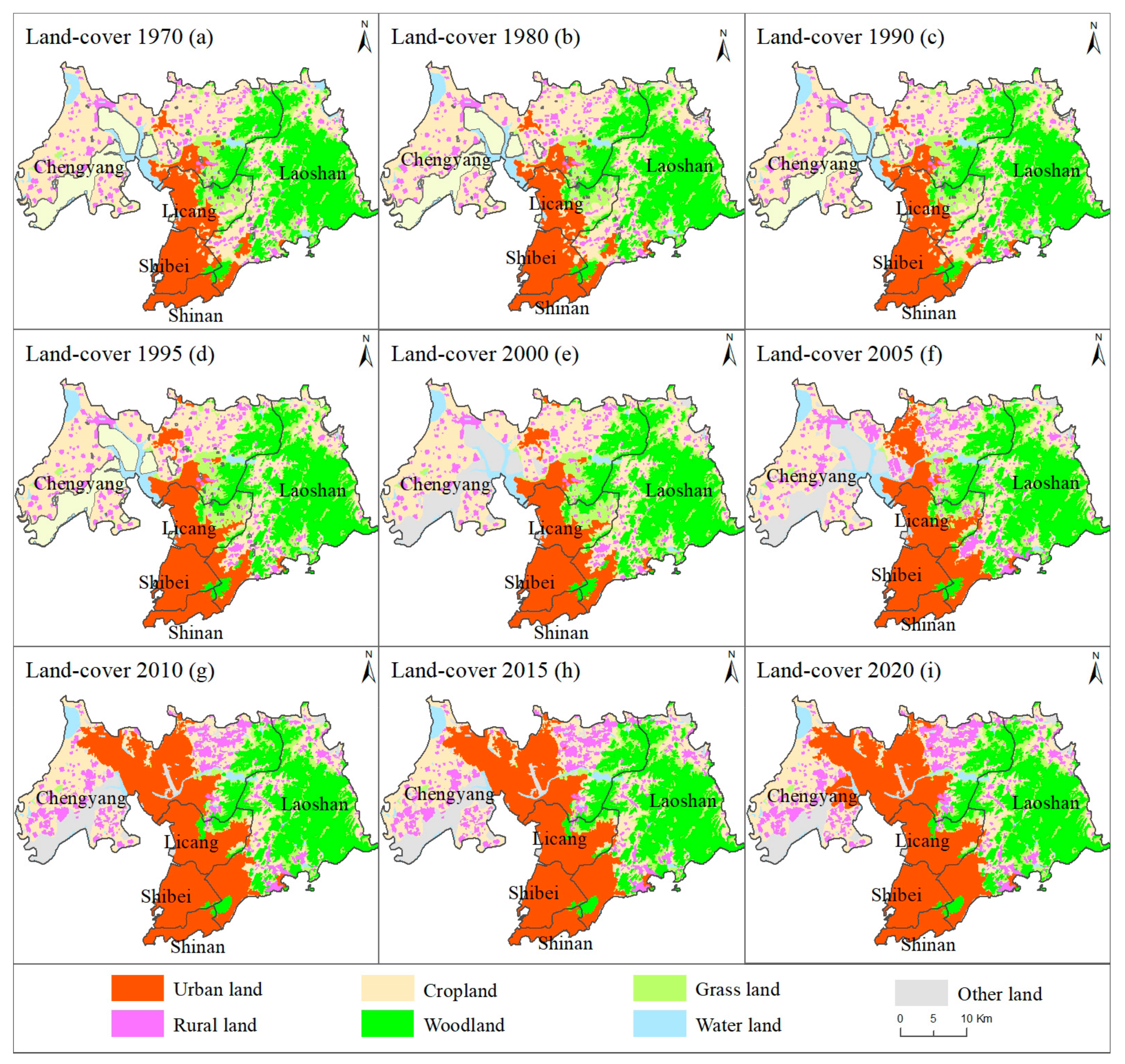
3.1. Analysis of Spatiotemporal Characteristics and Regional Differences in Urban and Rural Land Use from 1970 to 2020

3.1.1. Analysis of the Quantity and Spatial Change Characteristics of Urban and Rural Regions

The quantity of changes in urban and rural land showed a differential process in the past 50 years. In the initial year (i.e., 1970), the total urban–rural land area was 232.91 km2 (Figure 3), of which the urban and rural coverage areas were 158.90 km2 and 74.01 km2, respectively. Correspondingly, the ratios of these two land types were 68.22% and 31.78%, respectively. Then, for urban land, rapid urbanization was monitored in the past 50 years. The urban land area reached a total area of 367.52 km2 in the final year (i.e., 2020), accompanied by an overall growth rate of 131.29%. From 1970 to 2020, the fastest urban expansion occurred between 2000 and 2005. Meanwhile, rural land reached a coverage area of 106.15 km2 during the 50 years, displaying a total growth rate of 43.42%. This suggests that rural expansion accounted for 33.07% of the urban expansion in this region. Furthermore, unlike the continuous expansion of urban land, the quantity of rural land displayed a fluctuating feature of first rapidly increasing, then slightly decreasing, and then steadily increasing.
For the spatial change patterns, in 1970, urban land was mainly distributed in the southeast region of the study area, and the ratio of urban land to the entire region was 14.52%. To the west and south of the urban land was the ocean, which was very beneficial for improving the climate comfort level of the living environment and attracting tourists for sightseeing. After 1970, urban land underwent a continuous expansion process. The direction of expansion was to advance northwards due to the spatial constraints inherent to the geographical location. In addition to the oceans in the western and southern regions, which cannot undergo large-scale urban expansion, the Laoshan Mountains in the eastern region hinder urban expansion. Therefore, large-scale urban expansion can extend only northwards, from the Shinan District to Shibei District and then to the Licang and Chengyang Districts. During 1970–2020, the spatial pattern of the urban land gradually extended from the southwest portion of the research area to the north, forming an expansion concept of the central axis, which divided the research area evenly and symmetrically on the west and east sides.
Meanwhile, for the rural land, in 1970, the rural settlements were mainly distributed in scattered points. Then, the rural land in the research area underwent a transition from thatched houses to brick and tile houses. This has brought about a trend of rural settlements expanding from the original residential areas to the surrounding areas, such as the spread of cakes in rural regions. Rural settlements gradually expanded, and some villages were already interconnected, forming large villages in 2020. However, villages that were closer to urban land were engulfed by urban expansion and disappeared. Therefore, for land use monitoring, the time series of urban–rural changes displayed that the expansion ratios of urban and rural areas were 131.29% and 43.42% in the past 50 years, accompanied by differentiated spatial patterns.

3.1.2. Analysis of the Differences in Urban–Rural Land Use in Different Administrative Districts

The analysis of different administrative regions can further clarify the differences in the original land type background and its change process of urban–rural land. In 1970, the maximum value of the ratio of urban land in the corresponding administrative region occurred in Shibei District and Shinan District (Table 1), namely, 89.63% and 82.52%, respectively. This implied that the entire area was essentially covered by urban land, followed by the Licang District (i.e., 45.12%). Low values appeared in the Chengyang and Laoshan Districts, and both regions were less than 10%.
In the past 50 years, each administrative district underwent a different urban expansion process. Due to the suitable environment and unconstrained terrain conditions, Chengyang District had the largest increase in urban land area. This has led to an increase in the proportion of urban land in administrative divisions from 4.35% in 1970 to 30.73% in 2020, a change of 26.39%. The Licang and Laoshan Districts experienced similar urban land expansion, along with ratio increases of 33.65% and 7.77%, respectively. Meanwhile, the Shibei and Shinan Districts exhibited the changing ratio increments of 8.00% and 13.84%; the ratios of urban land in the corresponding administrative region were up to 97.63% and 96.36% in the Shibei and Shinan Districts, respectively. These two administrative regions were basically covered by urban land in 2020. For the rural land ratio changes in the different administrative regions, the increase in rural areas was generally low. The changing ratio of rural land in its administrative region was 4.82% in Chengyang District, 2.16% in Laoshan District. In contrast, the corresponding value was −1.55% in Licang District due to urban land expansion and the restricted administrative area during 1970–2020.

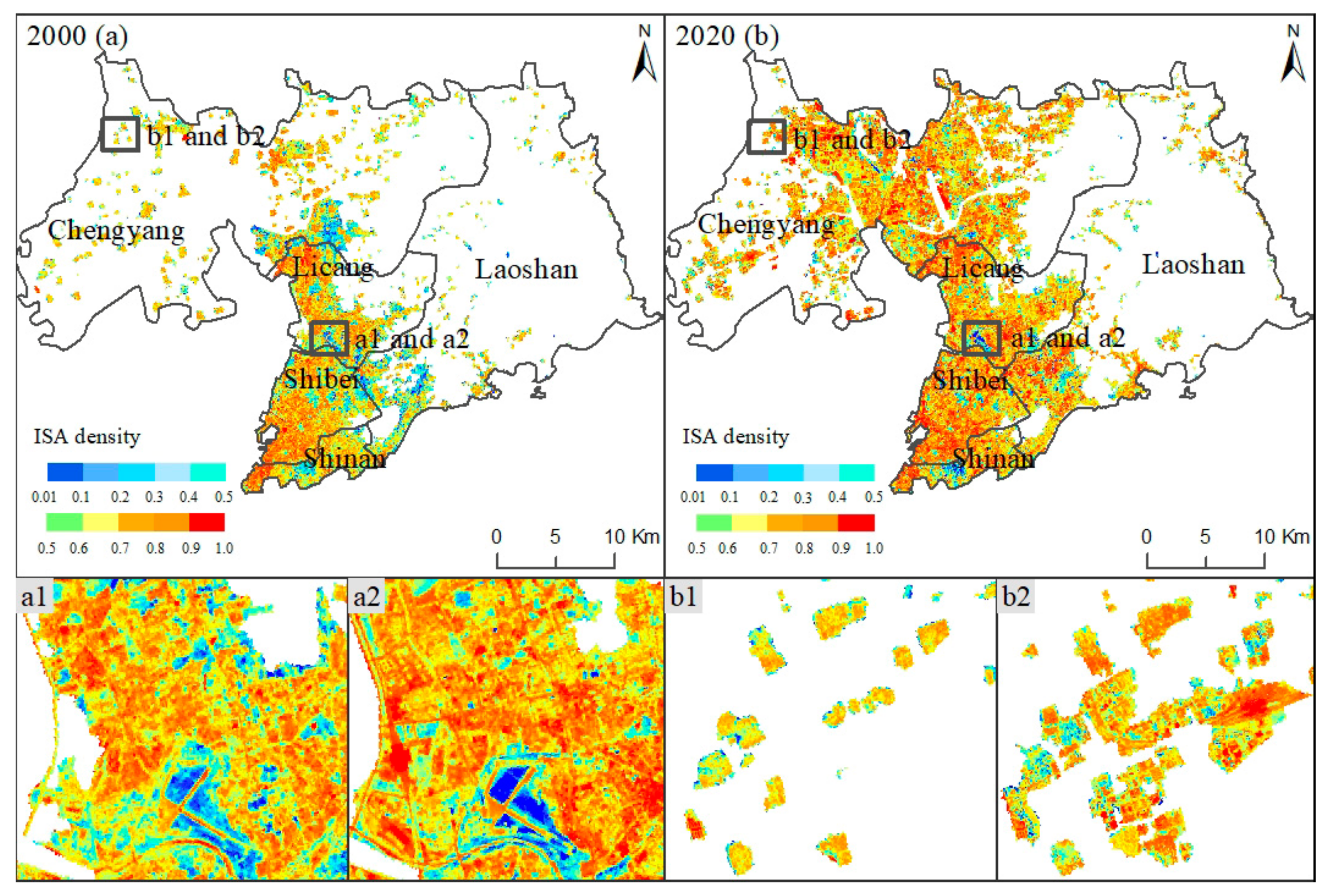
3.2. Analysis of the Spatiotemporal Pattern of Urban–Rural Impervious Surface Area

In the initial year, the total cover of the ISA was 173.16 km2, accounting for 15.85% of the whole study area (Figure 4). The ISA covers in urban and rural regions were 126.18 km2 and 46.98 km2, along with the average ISA densities of 63.43% and 62.63%, respectively. The data displayed that the average ISA density of urban regions was slightly higher than that of rural regions, with a difference between the two of 0.70.
From 2000 to 2020, China’s urban and rural regions underwent a rapid development process, along with periodic policies. As of 2003, real estate has become an important pillar industry of the national economy, effectively promoting the rise of concrete building structures in urban regions. In 2006, the national implementation of the “Village-to-Village Highway” project led to a significant expansion in rural regions of hardened roads with asphalt or cement pavement surfaces. The construction goals of international port cities, China’s megacities, and coastal central cities have improved Qingdao’s infrastructure and vastly improved its level of construction. In the context of the rapid modernization of urban and rural infrastructure, there was large-scale growth of ISA.
By the end of the year, the ISA covers increased by 168.59 km2, reaching 341.74 km2. The ratio of this ISA value to the whole study area was 31.24%, indicating a total ISA increment ratio of 97.36% compared to the ISA ratio in the initial year in the whole study area. Meanwhile, the ISA in urban and rural regions increased by 140.55 km2 and 28.04 km2, along with the average ISA densities of 72.57% and 70.67%, respectively. Therefore, the increments of average ISA density per unit pixel of urban and rural areas were 9.14% and 7.94%. A synchronous increase in both the urban and rural ISA was observed. The increased changes in urban ISA were relatively higher than those of the rural region at the pixel scale, with a different value of 1.20%.

3.3. Analysis of the Response Characteristics of Urban–Rural Impervious Surface Area to Land Surface Temperature

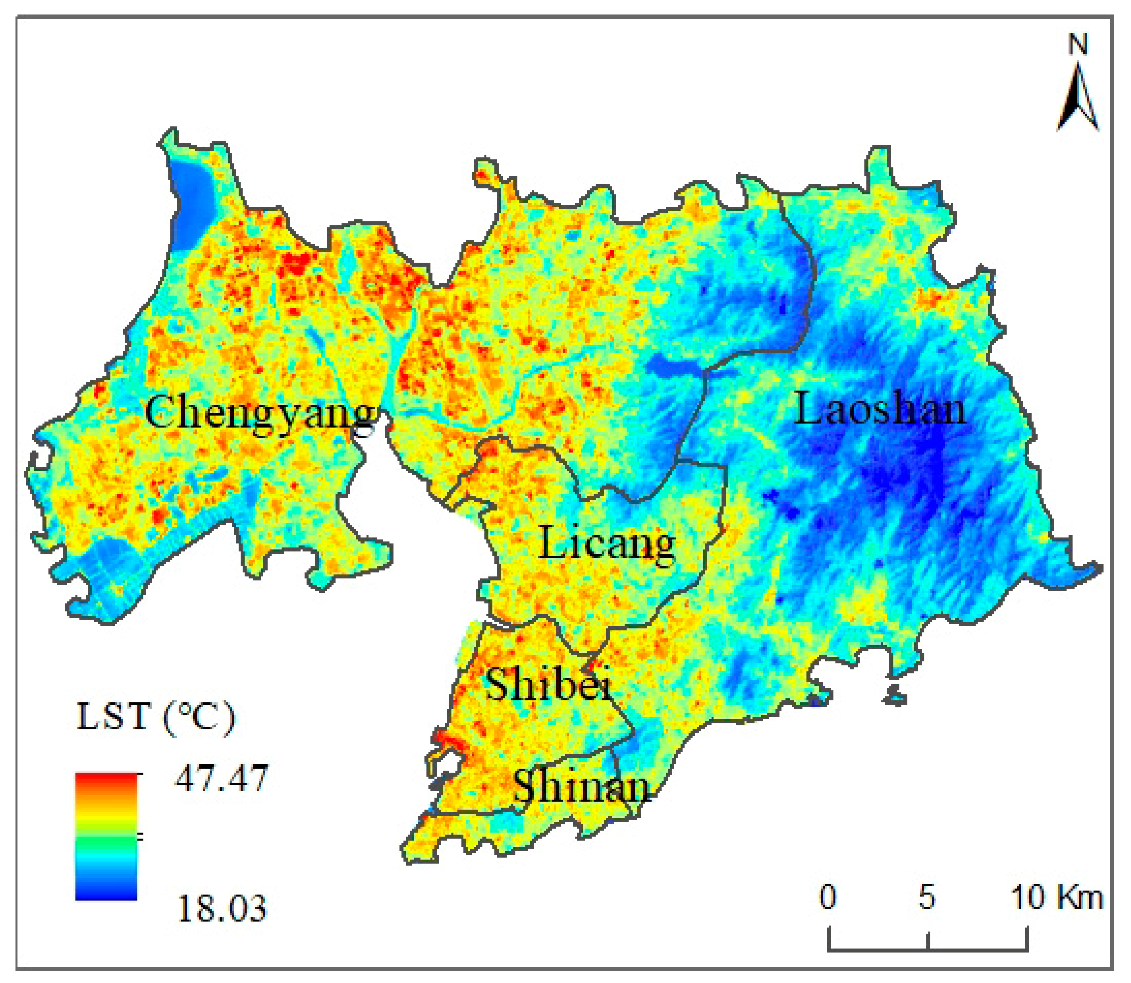
3.3.1. Analysis of Land Surface Temperature in the Whole Region and in Different Administrative Regions

Considering the differences in the meteorological and environmental conditions during different periods and further avoiding systematic temperature errors, we used only remote sensing images from the summer of 2020 as an example to retrieve and compare the LST. The range of the LST change throughout the entire research area was 18.03–47.47 °C. According to the investigation, the lowest LST mainly occurred in the lake areas, while the highest LST occurred in the large, concentrated ISA area. The average LST of the entire study area was 29.47 °C, showing a relative coolness compared to inland regions at the same latitude or the southern regions in China.
The LST also displayed differentiation across various urbanization-level areas. In the old, traditionally urban areas, namely, the Shinan and Shibei Districts, the average surface temperatures of these two regions were generally higher than those of other districts, with values of 29.75 °C in Shinan and 31.20 °C in Shibei (Figure 5), due to the existence of a large amount of urban and rural construction land in 1970 and coupling with the urbanization process from 2000 to 2020. However, the highest temperature occurred in the Chengyang District (i.e., 47.47 °C), although its average surface temperature was 29.10 °C, which was lower than that of the Shinan and Shibei Districts. Through investigation, it can be concluded that the large cover of ISA in the central and northern parts of Chengyang District had a strong LST aggregation effect, resulting in the highest temperature in the whole region, but the lowest temperature also occurred in this region due to the presence of lakes in the eastern part, which made the average LST in the region not high. The lowest average temperature appeared in the Laoshan District because of the presence of the Laoshan Mountains, where dense mountain forests formed a large low-temperature zone. In summary, the average LSTs at the district level, listed from high to low, were Shibei, Shinan, Licang, Chengyang and Laoshan, along with patterns of higher average temperature in the central axis in the north–south direction and lower values on both sides of the study area.

3.3.2. Comparison of the Differences in Land Surface Temperature between Urban and Rural Regions

The same temperature classification standard can effectively depict the difference between urban and rural regions. In this study, the LST was divided into five categories, namely, extremely low-temperature areas (<20 °C), low-temperature areas (20–25 °C), medium-temperature areas (25–35 °C), high-temperature areas (35–40 °C) and extremely high-temperature areas (≥40 °C), to compare the differences between urban and rural regions.
The statistical table shows that the LST in both urban and rural regions was mainly covered by medium-temperature areas, with corresponding coverage areas of 338.42 km2 and 100.93 km2, which accounted for 92.18% and 95.22% of the total area of urban and rural regions (Table 2), respectively. The data showed that the ratio of medium-temperature areas in rural regions was higher than that in urban regions. This can be attributed to the higher density of the ISA in the urban region, resulting in stronger temperature aggregation, and thus, the ratio of the high-temperature area in the urban region was 6.69% (i.e., 24.55 km2), which was obviously higher than that (3.77%, i.e., 4 km2) of the rural region. Similar results were also observed in extremely high-temperature areas of urban and rural regions, with corresponding ratios of 0.21% (i.e., 0.79 km2) and 0.07% (i.e., 0.07 km2), respectively. From another perspective, although extremely high-temperature regions were much lower in the rural regions than in the urban regions, there was also a high degree of ISA aggregation in the rural regions, resulting in the emergence of extremely high-temperature regions. For the low-temperature and extremely low-temperature regions, the summed ratio of the two categories accounted for approximately 0.9% of the area in both the urban regions and the rural regions, respectively, which was relatively close. Therefore, there were significant differences between the urban and rural regions in each LST classification.

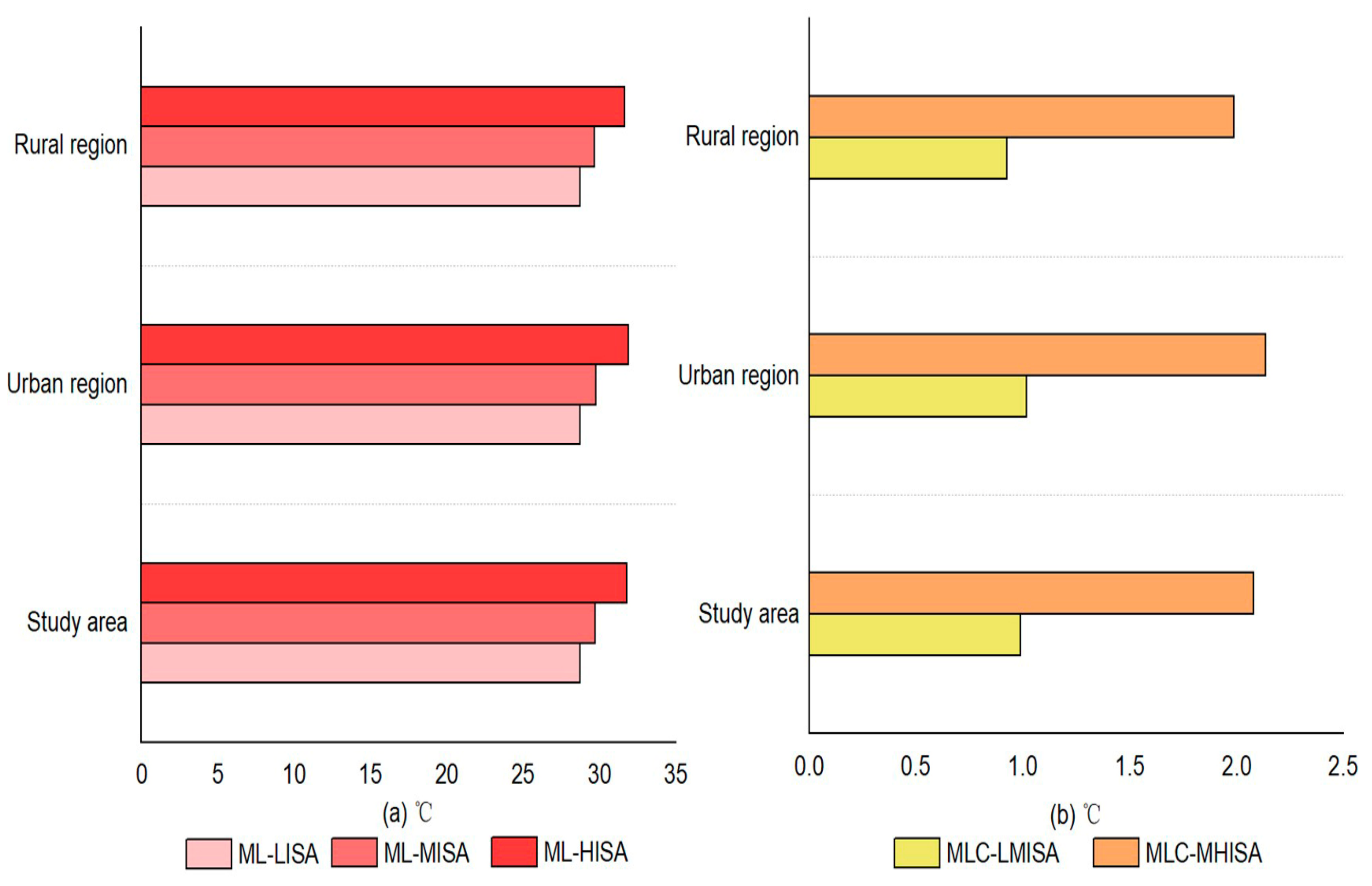
3.3.3. Response Characteristics of Urban and Rural Land Surface Temperature to Impervious Surface Area

To facilitate the exploration of the LST response of different ISA levels, the ISA was merged into three categories, including low-density ISA (i.e., ISA component from [0.001%, 33.33%)), medium-density ISA (i.e., ISA component from [33.33%, 66.66%)) and high-density ISA (i.e., ISA component from [66.66%, 100%]), according to the isodensity approach. Overall, the LST displayed an increasing trend as the ISA coverage increased. Specifically, in the low-density ISA area, the mean LST was 28.74 °C. Then, in the medium- and high-ISA areas, the mean LSTs were 29.73 °C and 31.81 °C, respectively. The data indicated that the difference values of the mean LST were continuously increasing, and the contribution of the ISA to the LST displayed an accelerating upward feature as the ISA changed from low- to medium- and from medium- to high-density areas, which provided the overall and quantitative LST differences under different ISA levels in the central coastal region of China.
In the urban and rural regions, there were differences in the effects of LST on ISA changes. At the same ISA level, for low-, medium-, and high-density ISA areas, the corresponding mean LSTs in the urban regions were 28.75 °C, 29.77 °C and 31.91 °C, respectively; at the same time, these values were 28.73 °C, 29.66 °C and 31.65 °C in the rural regions (Figure 6). The data showed that the LST in rural regions was slightly lower than that in urban regions at the same ISA level. This may be because of the aggregated LST effect of large-scale ISA and the obstruction effect on the airflow from tall buildings in urban regions. In contrast, in rural regions, the size of the ISA was relatively small, and the building height was generally low, making the heat easily spread to the surrounding areas from the villages. This can be called the horizontal gradient effect of the LST from urban to rural regions. Furthermore, at different ISA levels, the change in the ISA was 1.02 °C and 2.14 °C in the urban region, while it was 0.93 °C and 1.99 °C in the rural region during the changing process from low- to medium- and from medium- to high-density ISA, respectively. The data showed that the different LST values between urban and rural regions at different ISA levels gradually increased. Therefore, the LST in the cities was slightly higher than that in the villages, whether at the same or different ISA levels. The horizontal gradient effect of the LST from urban to rural regions was also first reported.

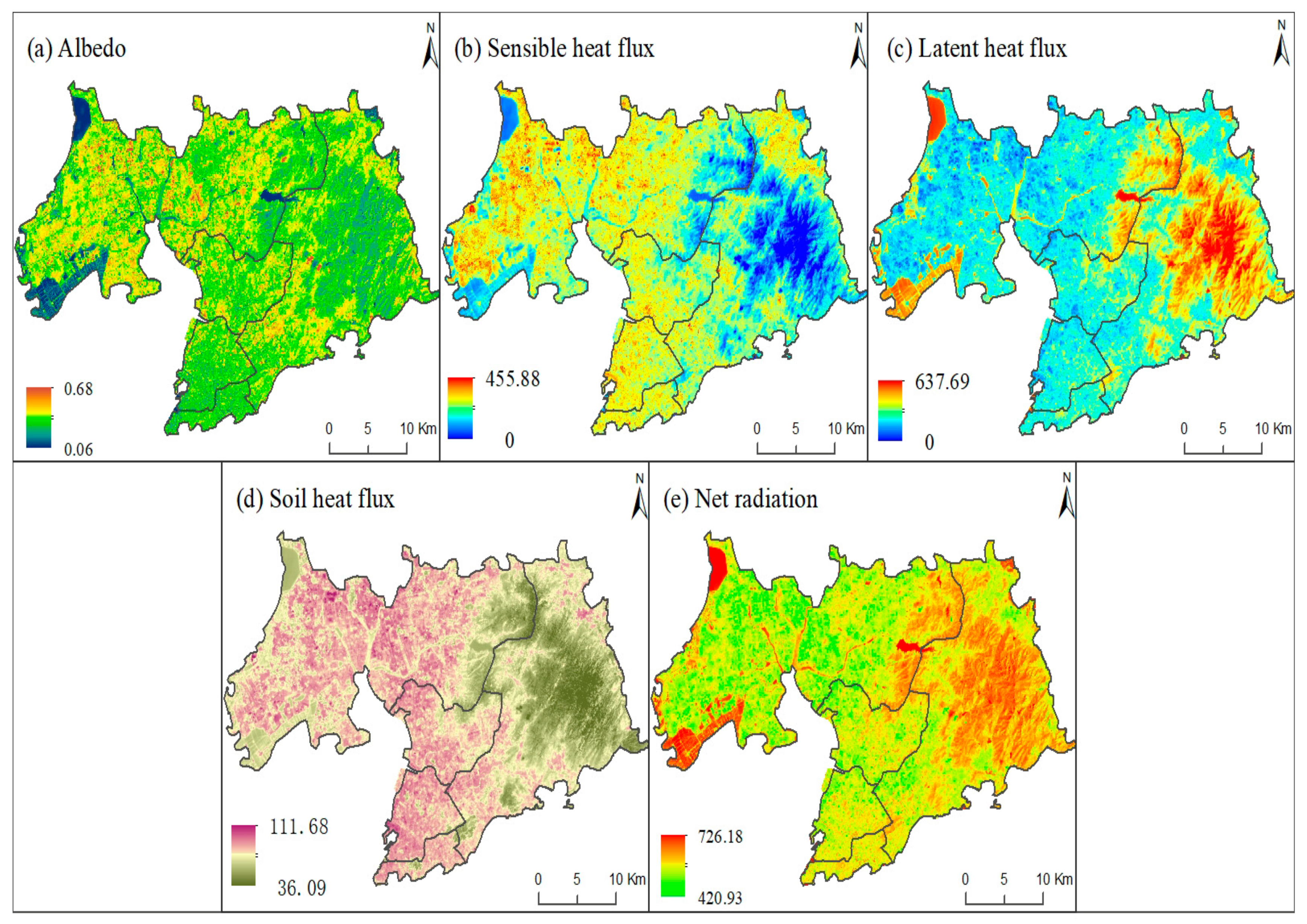
3.4. Mechanism Analysis of LST Response to ISA Changes in Urban and Rural Regions

This section focuses on the response mechanism between the ISA and the LST through the radiation balance and the energy balance equation of the land surface. The land surface received visible and near-infrared radiation from sunlight, triggering land thermal infrared wave radiation. The thermal radiation was absorbed through water vapor and carbon dioxide near the ground, heating the air near the ground. The surface roughness of different land-cover types varied: ISA expansion into surrounding green lands and water bodies in urban and rural regions disrupted the air near the surface, generating air turbulence. The albedo (i.e., the characteristic of the surface roughness, Figure 7a) of the urban region was lower than that of the rural region. The low albedo in urban regions implied that more heat was absorbed by the ground, leading to more air turbulence being transferred from the ground to the near-surface air. These air turbulences transported the near-surface hot air upwards. The upwelling airflow then mixed with local horizontal advection, causing an increase or decrease in the LST. More expansion of the ISA in the urban areas brought more upward air turbulence, which can be described as the sensible heat flux because sensible heat flux is usually considered the amount of heat that we can directly feel from the surrounding environments. Therefore, the sensible heat flux (Figure 7b) was higher in the urban regions than in the rural regions, with corresponding values of 280.13 W/m2 and 274.76 W/m2, respectively. More sensible heat flux release often leads to less latent heat flux stored on the land surface. Based on model simulation and statistical results, less latent heat flux (Figure 7c) was displayed in the urban region (174.71 W/m2) than in the rural region (180.20 W/m2). The data showed that in the changing process of this mechanism, more heat energy developed in the urban regions, indicating a more acute LST response to the ISA changes in the urban than in the rural regions.

4. Discussion

4.1. The Horizontal Gradient Effect and Vertical Density Effect of Land Surface Temperature on Impervious Surface Area in Urban and Rural Regions of Central Coastal Region of China

An analysis of the spatiotemporal expansion pattern of the ISA and its response characteristics to the LST from the perspective of synchronous urban–rural changes was first performed in the central coastal region of China; this research can compensate for the lack of research on urban and rural ISA and LST changes from different dimensions (i.e., the horizontal gradient effect and the vertical density effect). The findings showed that at the same ISA level (i.e., the horizontal gradient effect), the mean LSTs were 28.75 °C, 29.77 °C and 31.91 °C in the urban regions and 28.73 °C, 29.66 °C and 31.65 °C in the rural regions (Figure 4 and Figure 5) from the low-, medium-, and high-density ISA areas, respectively, displaying gradually increasing differences of 0.02 °C, 0.11 °C, and 0.26 °C. At the different ISA levels (i.e., the vertical density effect), the changes in the LST were 1.02 °C and 2.14 °C in the urban region, while they were 0.93 °C and 1.99 °C in the rural region during the changing process from the low- to medium- and from the medium- to high-density ISA. The findings showed that the response values of the LST to the ISA in the urban regions were higher than those in the rural regions, both horizontally and vertically; the quantitative values were provided for this study. In the horizontal direction, the high-density ISA of cities meets the needs of commercial, residential, and public transportation [45,46] for many urban residents, and large areas of ISA often lead to higher temperature aggregation effects compared to rural areas, where the rural boundaries are relatively small and the ISA density is slightly lower [47]. In the vertical direction, the dense high-rise buildings in urban areas have a certain blocking effect on the horizontal air turbulence, causing temperatures to rise more vertically and forming a relatively high heat island effect [9,48]. Compared to this phenomenon, buildings in rural settlements were generally lower and more susceptible to wind and other factors.
The comparative study on the response changes in the LST to the ISA in urban and rural regions had many practical values. First, the comparison of the differences in the ISA structure between urban and rural areas helped in understanding the impacts of hardening urban and rural roads, home construction, and the density of community buildings [49] while also indirectly reflecting the greening situation in urban and rural regions, as demonstrated through community planning maps (i.e., the layout of the ISA and green spaces) [46,49]. Second, the differences in the energy aggregation between the urban and rural regions can be compared to provide a reference for relevant research in other regions, considering that the total amount of solar radiation that each region can receive is different. As in Harbin, located in a cold temperate zone of Northeast China [50,51], the LST polymerization from the LST was weaker than in our research area, the central coastal region of China and the warm temperate zone. Third, the development of tourism for the whole territory should be promoted. The comfort level of the residential thermal environment is often a significant factor that tourism management departments and tourists need to consider because extremely high temperatures and heatwaves often make people feel uncomfortable [52]. Through spatial mappings of the ISA and the LST, as well as their corresponding energy analysis in urban and rural regions, management departments can effectively understand the ISA and energy distribution of urban and rural regions and establish reasonable urban and rural tourism routes to provide tourists with a very good tourism experience while ensuring the comfort level of the thermal environments.

4.2. Differences in Characteristic Patterns of Urban Impervious Surface Areas in Different Regions and Potential Eco-Environmental Effects

Currently, there have been many studies on the ISA in different regions [9,47,53], which have displayed different characteristics. In this study, the evaluated ratio of the ISA to its built-up area was 63.43% in 2000 and 72.57% in 2020, showing an increase of 9.14% in the ratio of the ISA in urban regions (Figure 4). This value was reflected not only in the old urban area but also in the difference across the whole region in the average ISA ratio of the built-up area in 2000 and 2020, displaying a drastic pattern of ISA spatiotemporal change. Similarly, in Harbin, another megacity in the same region (i.e., Northern China), the ratio of the ISA to the built-up area was 43.92% in 2001 [54]. This value was much lower than the corresponding ISA ratio in the initial year of this study. Then, the ratio of the ISA in Harbin increased to 49.14% by 2015, with an average annual growth ratio of 0.348% from 2000 to 2015 [54], which was also lower compared to our research area (which had an average annual growth ratio of 0.457%). The data showed that the growth rate of ISA in our research area was higher than that in this megacity in northern China.
Furthermore, the ISA comparison of our study city with a higher-level city (i.e., Beijing, one of the six highest-level cities, the capital city and political, economic, and external centre of China) was conducted in Northern China. The ISA ratio was 65.9% in 1981 and 73.9% in 2021 [46], showing an annual average increment rate of 0.2% from 1981 to 2021, which accounted for only half of the ISA growth rate in our research area. This may be due to the high ratio of ISA in Beijing in 1981 [46], which was higher than that of our study area (i.e., 65.9% in 1981 in Beijing vs. 63.3% in 2000 in Qingdao), and the further increment of ISA space was limited in Beijing, considering the impact of retaining a portion of residential green environment land within the built-up area [46,47].
In addition to comparing the spatiotemporal heterogeneity of ISA in northern China, the differences in ISA change under different climate backgrounds should also be compared in all of China. Our research area was located along the central coast of China in the humid climate zone. Therefore, the ISA of cities in the arid climate zone, Urumqi, the largest city in China’s arid climate zone [55], was considered in this study. The ratio of ISA in built-up areas was 63.20% in 2000 and 73.56% in 2015 [56], and the ratio of ISA in Urumqi was higher than that in our study area. According to our investigation, the urban buildings in Urumqi were mainly compact, and the vegetation greening was relatively low in this arid climate [55,56]. However, our research area was located in a coastal area, and there was a large amount of vegetation in the city for ecological systems. The city’s ISA and green spaces were more like a mosaic pattern to enhance the comfort level of the living environments.
For the eco-environmental effects of ISA, the changes in ISA can first bring about water environmental effects [57,58]. The rapid expansion of ISA changed the surface hydrological process. The speed and peak value of surface runoff formed by rainfall were much higher in regions with high ISA than in those with low ISA. Large runoff in the rainstorm season was prone to overflow pollution, and nonpoint source pollution led to changes in the indicators of dissolved oxygen, ammonia nitrogen, total phosphorus, chemical oxygen demand, etc. [59,60,61]. Therefore, it is necessary to regulate and manage the threshold effect of watershed ecosystems and nonpoint source pollution in areas with high ISA expansion or concentrated ISA regions. Another environmental effect of ISA was energy [62]. As is well known, the accumulation of ISA often brings about urban heat island effects in hot summers in humid regions [63]. In contrast, in arid regions, the larger thermal capacity of sand allows it to display higher temperatures compared to ISA, forming a cold island effect in ISA regions [64,65,66].

4.3. Rural Settlements in China Experienced Drastic Structural Evolution

Although this study found that increases in the ISA area in urban regions were greater than those in rural regions, the expansion of the ISA in rural regions in our study area was still very intense. This was different from the rural settlements in Europe [53], where the spatial structure of the rural settlements was basically stable and there were few large/acute changes [53,67]. Furthermore, in this study, a new finding was found with the dual effects of the ISA in rural areas, namely, the horizontal expansion effect of the acute ISA expansion outside the original village boundaries and the vertical rise effect of the increased ISA density within the original village boundaries, implying dramatic horizontal and vertical ISA evolutionary processes in the rural settlement structure of the study area. In fact, the evolution of the rural settlements in the research area was a microcosm/sample of the rural changes in China [68,69].
Since 1970, China strived to solve the basic problem of food and clothing for its people. After China joined the World Trade Organization in 2001 [70], its economy grew rapidly. In this process, the income of farmers also clearly increased. Through these individual incomes, many original earthen houses were demolished, and large tiled houses have sprung up one by one [71,72]. This indicates that the living standards of rural residents have been upgraded. In addition to improving the village environment by the farmers themselves, the Chinese government implemented a series of rural policies, such as the “Village-to-Village Connection Project” [73], which includes roads, electricity, living and drinking water, telephone networks, cable television networks, and the internet. Among these, the village-to-village road project (i.e., the roads inside and outside the villages) aimed to construct asphalt or cement roads in all villages, to break the transportation bottleneck of rural economic development and to solve the travel challenges faced by farmers [73]. Under this background, the spatial ISA of rural areas rapidly increased.
Furthermore, the Chinese government further implemented the ‘rural revitalization strategy’, which further promoted spatial ISA structure changes, such as the construction of squares, elderly activity centers, hospitals and service stations within the village boundaries [74,75], to enhance rural life. At the same time, the central government of China is also testing policies for the construction of rural ecological civilization [76,77], such as greening in rural areas to enhance the comfort level of the rural living environment and to reasonably optimize the spatial layout of the ISA and greenery. Additionally, some rural issues, including the low population in Northeast China [78] and population aging throughout China [79], are also emerging and urgently need to be addressed to enhance rural development. Measures to remove small villages and merge them into large villages are also gradually being implemented [80,81]. These new issues and policies drive the need for obvious changes in the ISA structural patterns and the greening layout of rural areas in China, which will become the focus of our continuous attention to future rural issues in China.

4.4. Shortcomings and Prospects of Research

Although there were currently many studies on the impact of ISA on LST, there was still a lack of analysis from an urban–rural comparison perspective. This study investigated the ISA patterns and their response to the LST mechanism from an urban–rural synchronous comparison perspective in the Megacity, Qingdao, the coastal areas of China. For exploring the temperature mechanism, the indicators of surface energy radiation balance, including the latent heat flux, sensible heat flux, soil heat flux, and net radiation were calculated, using the PCACA model and TVDI model. But the city in the study area was single and there were insufficient manual observation experiments. For a more in-depth exploration in the future, more cities in different regions of China, such as Guangzhou in southern China, Beijing in northern China, Harbin in northeastern China, Urumqi in northwestern China, and Lanzhou in southwestern China, will be screened as the study area, to provide the synchronous comparison of the response characteristics of LST to ISA in urban and rural areas. For the method, more accurate micrometeorological modeling should be excavated, and more flux observation experiments should also be included, to provide more accurate results.

5. Conclusions

To solve the lack of the response of LST to ISA changes from an urban–rural synchronous comparison perspective in a central coastal megalopolis of China, this study took Qingdao as an example using the methodology of artificial digitization—fully constrained least squares mixed pixel decomposition—split-window algorithm—PCACA model. The main conclusions were below. Long time series of land use monitoring indicated that the expansion ratios of urban and rural areas were 131.29% and 43.42% in the past 50 years, accompanied by differentiated spatial patterns. Then, a synchronous ISA increase in both the urban and the rural regions was monitored, with the increment by 140.55 km2 and by 28.04 km2, separately. By 2020, the ISA increases in the urban regions were higher than those in the rural regions, but the patterns of the ISA in both regions exhibited similar features of horizontal epitaxial expansion and vertical density enhancement. For the response of LST to ISA, the aggregated LST effect was revealed, namely, the horizontal gradient effect displayed that the mean LSTs were 28.75 °C, 29.77 °C and 31.91 °C in the urban regions and 28.73 °C, 29.66 °C and 31.65 °C in rural regions from low-, medium-, and high-density ISA areas, respectively. The vertical density effect displayed that the changes in LST were 1.02 °C and 2.14 °C in the urban region, while they were 0.93 °C and 1.99 °C in the rural region during the changing process from low- to medium- and from medium- to high-density ISA, respectively. Meanwhile, the potential surface energy indicators were evaluated to explain the mechanism effect of the ISA changes on the LST in the urban and rural regions.
The main contribution of this study to the fields of land use, impervious surface area, land surface temperature, and surface energy radiation balance can be summarized below: (1) The long time series of spatiotemporal land change patterns were monitored in urban and rural areas in the past 50 years (i.e., 1970–2020). (2) The horizontal and vertical effects of the different ISA densities in urban and rural areas were revealed. And (3) the differences in surface thermal properties mechanism between urban and rural areas were calculated and compared.
This study was related to the contents of the current situation and challenges of urban development, one aspect of the Sustainable Development Goals (SDGs). The history of urban development over the past 50 years in this study was evaluated, which provided the basic reference for population urbanization for the year 2030 SDGs. Meanwhile, the thermal environmental effects of the different ISA densities were beneficial for urban planning departments and managers to provide important practical data for the layout of urban parks, block green spaces, and ecological corridor planning, serving the well-being of urban living and the harmonious of urban development and nature environments.

Author Contributions

Methodology, T.P.; Investigation, B.L.; Writing—original draft, T.P.; Writing—review & editing, T.P., B.L. and L.N. All authors have read and agreed to the published version of the manuscript.

Funding

This study is supported by Natural Science Foundation Youth Program of Shandong Province (grant no. ZR2021QD134 and ZR2021YQ28) and Taishan Scholars Project of Shandong Province (tsqn202306182).

Data Availability Statement

Not applicable.

Conflicts of Interest

The authors declare no conflict of interest.

References

  1. Li, Y.; Kong, X.; Zhu, Z. Multiscale analysis of the correlation patterns between the urban population and construction land in China. Sustain. Cities Soc. 2020, 61, 102326. [Google Scholar] [CrossRef]
  2. Li, Y. Urban–rural interaction patterns and dynamic land use: Implications for urban–rural integration in China. Reg. Environ. Chang. 2012, 12, 803–812. [Google Scholar] [CrossRef]
  3. Guan, X.; Wei, H.; Lu, S.; Dai, Q.; Su, H. Assessment on the urbanization strategy in China: Achievements, challenges and reflections. Habitat Int. 2018, 71, 97–109. [Google Scholar] [CrossRef]
  4. Kuang, W.; Liu, J.; Dong, J.; Chi, W.; Zhang, C. The rapid and massive urban and industrial land expansions in China between 1990 and 2010: A CLUD-based analysis of their trajectories, patterns, and drivers. Landsc. Urban Plan. 2016, 145, 21–33. [Google Scholar] [CrossRef]
  5. Gaughan, A.E.; Stevens, F.R.; Huang, Z.; Nieves, J.J.; Sorichetta, A.; Lai, S.; Ye, X.; Linard, C.; Hornby, G.M.; Hay, S.I. Spatiotemporal patterns of population in mainland China, 1990 to 2010. Sci. Data 2016, 3, 160005. [Google Scholar] [CrossRef] [PubMed]
  6. Wang, X.; Shi, R.; Zhou, Y. Dynamics of urban sprawl and sustainable development in China. Socio-Econ. Plan. Sci. 2020, 70, 100736. [Google Scholar] [CrossRef]
  7. Kuang, W.; Zhang, S.; Li, X.; Lu, D. A 30 m resolution dataset of China’s urban impervious surface area and green space, 2000–2018. Earth Syst. Sci. Data 2021, 13, 63–82. [Google Scholar] [CrossRef]
  8. Wu, W.; Li, C.; Liu, M.; Hu, Y.; Xiu, C. Change of impervious surface area and its impacts on urban landscape: An example of Shenyang between 2010 and 2017. Ecosyst. Health Sustain. 2020, 6, 1767511. [Google Scholar] [CrossRef]
  9. Sekertekin, A.; Zadbagher, E. Simulation of future land surface temperature distribution and evaluating surface urban heat island based on impervious surface area. Ecol. Indic. 2021, 122, 107230. [Google Scholar] [CrossRef]
  10. Morabito, M.; Crisci, A.; Guerri, G.; Messeri, A.; Congedo, L.; Munafò, M. Surface urban heat islands in Italian metropolitan cities: Tree cover and impervious surface influences. Sci. Total Environ. 2021, 751, 142334. [Google Scholar] [CrossRef]
  11. Luo, Y.; Zhao, Y.; Yang, K.; Chen, K.; Pan, M.; Zhou, X. Dianchi Lake watershed impervious surface area dynamics and their impact on lake water quality from 1988 to 2017. Environ. Sci. Pollut. Res. 2018, 25, 29643–29653. [Google Scholar] [CrossRef] [PubMed]
  12. Yang, K.; Pan, M.; Luo, Y.; Chen, K.; Zhao, Y.; Zhou, X. A time-series analysis of urbanization-induced impervious surface area extent in the Dianchi Lake watershed from 1988–2017. Int. J. Remote Sens. 2019, 40, 573–592. [Google Scholar] [CrossRef]
  13. McGlynn, T.P.; Meineke, E.K.; Bahlai, C.A.; Li, E.; Hartop, E.A.; Adams, B.J.; Brown, B.V. Temperature accounts for the biodiversity of a hyperdiverse group of insects in urban Los Angeles. Proc. R. Soc. B 2019, 286, 20191818. [Google Scholar] [CrossRef] [PubMed]
  14. Yang, Q.; Huang, X.; Yang, J.; Liu, Y. The relationship between land surface temperature and artificial impervious surface fraction in 682 global cities: Spatiotemporal variations and drivers. Environ. Res. Lett. 2021, 16, 024032. [Google Scholar] [CrossRef]
  15. Zhang, Y.; Sun, L. Spatial-temporal impacts of urban land use land cover on land surface temperature: Case studies of two Canadian urban areas. Int. J. Appl. Earth Obs. Geoinf. 2019, 75, 171–181. [Google Scholar] [CrossRef]
  16. Yang, J.; Jin, S.; Xiao, X.; Jin, C.; Xia, J.C.; Li, X.; Wang, S. Local climate zone ventilation and urban land surface temperatures: Towards a performance-based and wind-sensitive planning proposal in megacities. Sustain. Cities Soc. 2019, 47, 101487. [Google Scholar] [CrossRef]
  17. Vancutsem, C.; Ceccato, P.; Dinku, T.; Connor, S.J. Evaluation of MODIS land surface temperature data to estimate air temperature in different ecosystems over Africa. Remote Sens. Environ. 2010, 114, 449–465. [Google Scholar] [CrossRef]
  18. Guo, A.; Yang, J.; Sun, W.; Xiao, X.; Cecilia, J.X.; Jin, C.; Li, X. Impact of urban morphology and landscape characteristics on spatiotemporal heterogeneity of land surface temperature. Sustain. Cities Soc. 2020, 63, 102443. [Google Scholar] [CrossRef]
  19. Yang, J.; Zhan, Y.; Xiao, X.; Xia, J.C.; Sun, W.; Li, X. Investigating the diversity of land surface temperature characteristics in different scale cities based on local climate zones. Urban Clim. 2020, 34, 100700. [Google Scholar] [CrossRef]
  20. Estoque, R.C.; Murayama, Y.; Myint, S.W. Effects of landscape composition and pattern on land surface temperature: An urban heat island study in the megacities of Southeast Asia. Sci. Total Environ. 2017, 577, 349–359. [Google Scholar] [CrossRef]
  21. Zhao, Z.; Sharifi, A.; Dong, X.; Shen, L.; He, B.-J. Spatial variability and temporal heterogeneity of surface urban heat island patterns and the suitability of local climate zones for land surface temperature characterization. Remote Sens. 2021, 13, 4338. [Google Scholar] [CrossRef]
  22. Liu, X.; Zhou, Y.; Yue, W.; Li, X.; Liu, Y.; Lu, D. Spatiotemporal patterns of summer urban heat island in Beijing, China using an improved land surface temperature. J. Clean. Prod. 2020, 257, 120529. [Google Scholar] [CrossRef]
  23. Ren, T.; Zhou, W.; Wang, J. Beyond intensity of urban heat island effect: A continental scale analysis on land surface temperature in major Chinese cities. Sci. Total Environ. 2021, 791, 148334. [Google Scholar] [CrossRef] [PubMed]
  24. Huang, F.; Yu, Y.; Feng, T. Automatic extraction of impervious surfaces from high resolution remote sensing images based on deep learning. J. Vis. Commun. Image Represent. 2019, 58, 453–461. [Google Scholar] [CrossRef]
  25. Wang, Y.; Li, M. Urban impervious surface detection from remote sensing images: A review of the methods and challenges. Ieee Geosci. Remote Sens. Mag. 2019, 7, 64–93. [Google Scholar] [CrossRef]
  26. Zhao, J.; Tsutsumida, N. Mapping Fragmented Impervious Surface Areas Overlooked by Global Land-Cover Products in the Liping County, Guizhou Province, China. Remote Sens. 2020, 12, 1527. [Google Scholar] [CrossRef]
  27. Tang, Y.; Shao, Z.; Huang, X.; Cai, B. Mapping impervious surface areas using time-series nighttime light and MODIS imagery. Remote Sens. 2021, 13, 1900. [Google Scholar] [CrossRef]
  28. Phinn, S.; Stanford, M.; Scarth, P.; Murray, A.; Shyy, P. Monitoring the composition of urban environments based on the vegetation-impervious surface-soil (VIS) model by subpixel analysis techniques. Int. J. Remote Sens. 2002, 23, 4131–4153. [Google Scholar] [CrossRef]
  29. Ridd, M.K. Exploring a VIS (vegetation-impervious surface-soil) model for urban ecosystem analysis through remote sensing: Comparative anatomy for cities. Int. J. Remote Sens. 1995, 16, 2165–2185. [Google Scholar] [CrossRef]
  30. Yue, W. Improvement of urban impervious surface estimation in Shanghai using Landsat7 ETM+ data. Chin. Geogr. Sci. 2009, 19, 283–290. [Google Scholar] [CrossRef]
  31. Wang, J.; Wu, Z.; Wu, C.; Cao, Z.; Fan, W.; Tarolli, P. Improving impervious surface estimation: An integrated method of classification and regression trees (CART) and linear spectral mixture analysis (LSMA) based on error analysis. Gisci. Remote Sens. 2018, 55, 583–603. [Google Scholar] [CrossRef]
  32. Cristóbal, J.; Jiménez-Muñoz, J.C.; Prakash, A.; Mattar, C.; Skoković, D.; Sobrino, J.A. An improved single-channel method to retrieve land surface temperature from the Landsat-8 thermal band. Remote Sens. 2018, 10, 431. [Google Scholar] [CrossRef]
  33. Sahana, M.; Ahmed, R.; Sajjad, H. Analyzing land surface temperature distribution in response to land use/land cover change using split window algorithm and spectral radiance model in Sundarban Biosphere Reserve, India. Model. Earth Syst. Environ. 2016, 2, 81. [Google Scholar] [CrossRef]
  34. Du, C.; Ren, H.; Qin, Q.; Meng, J.; Zhao, S. A practical split-window algorithm for estimating land surface temperature from Landsat 8 data. Remote Sens. 2015, 7, 647–665. [Google Scholar] [CrossRef]
  35. Liu, K.; Su, H.; Li, X. Comparative assessment of two vegetation fractional cover estimating methods and their impacts on modeling urban latent heat flux using Landsat imagery. Remote Sens. 2017, 9, 455. [Google Scholar] [CrossRef]
  36. Liu, J.; Kuang, W.; Zhang, Z.; Xu, X.; Qin, Y.; Ning, J.; Zhou, W.; Zhang, S.; Li, R.; Yan, C. Spatiotemporal characteristics, patterns, and causes of land-use changes in China since the late 1980s. J. Geogr. Sci. 2014, 24, 195–210. [Google Scholar] [CrossRef]
  37. Zhang, Z.; Wang, X.; Zhao, X.; Liu, B.; Yi, L.; Zuo, L.; Wen, Q.; Liu, F.; Xu, J.; Hu, S. A 2010 update of National Land Use/Cover Database of China at 1: 100000 scale using medium spatial resolution satellite images. Remote Sens. Environ. 2014, 149, 142–154. [Google Scholar] [CrossRef]
  38. Xu, Y.; Yu, L.; Peng, D.; Zhao, J.; Cheng, Y.; Liu, X.; Li, W.; Meng, R.; Xu, X.; Gong, P. Annual 30-m land use/land cover maps of China for 1980–2015 from the integration of AVHRR, MODIS and Landsat data using the BFAST algorithm. Sci. China Earth Sci. 2020, 63, 1390–1407. [Google Scholar] [CrossRef]
  39. Liu, Y.; Zhong, Y.; Ma, A.; Zhao, J.; Zhang, L. Cross-resolution national-scale land-cover mapping based on noisy label learning: A case study of China. Int. J. Appl. Earth Obs. Geoinf. 2023, 118, 103265. [Google Scholar] [CrossRef]
  40. Ning, J.; Liu, J.; Kuang, W.; Xu, X.; Zhang, S.; Yan, C.; Li, R.; Wu, S.; Hu, Y.; Du, G. Spatiotemporal patterns and characteristics of land-use change in China during 2010–2015. J. Geogr. Sci. 2018, 28, 547–562. [Google Scholar] [CrossRef]
  41. Heylen, R.; Burazerovic, D.; Scheunders, P. Fully constrained least squares spectral unmixing by simplex projection. IEEE Trans. Geosci. Remote Sens. 2011, 49, 4112–4122. [Google Scholar] [CrossRef]
  42. Yin, C.; Meng, F.; Yu, Q. Calculation of land surface emissivity and retrieval of land surface temperature based on a spectral mixing model. Infrared Phys. Technol. 2020, 108, 103333. [Google Scholar] [CrossRef]
  43. Rozenstein, O.; Qin, Z.; Derimian, Y.; Karnieli, A. Derivation of land surface temperature for Landsat-8 TIRS using a split window algorithm. Sensors 2014, 14, 5768–5780. [Google Scholar] [CrossRef] [PubMed]
  44. Liu, K.; Su, H.; Wang, W.; Yang, L.; Liang, H.; Li, X. Comparative assessment of Two Source of Landsat TM vegetative fraction coverage for modeling urban latent heat fluxes. In Proceedings of the 2016 IEEE International Geoscience and Remote Sensing Symposium (IGARSS), Beijing, China, 10–15 July 2016; pp. 6762–6765. [Google Scholar]
  45. Zhang, T.; Xiao, Y.; Liang, D.; Tang, H.; Xu, J.; Yuan, S.; Luan, B. A physically-based model for dissolved pollutant transport over impervious surfaces. J. Hydrol. 2020, 590, 125478. [Google Scholar] [CrossRef]
  46. Pan, T.; Kuang, W.; Pan, R.; Niu, Z.; Dou, Y. Hierarchical Urban Land Mappings and Their Distribution with Physical Medium Environments Using Time Series of Land Resource Images in Beijing, China (1981–2021). Remote Sens. 2022, 14, 580. [Google Scholar] [CrossRef]
  47. Peng, J.; Liu, Y.; Ma, J.; Zhao, S. A new approach for urban–rural fringe identification: Integrating impervious surface area and spatial continuous wavelet transform. Landsc. Urban Plan. 2018, 175, 72–79. [Google Scholar] [CrossRef]
  48. Mathew, A.; Khandelwal, S.; Kaul, N. Spatial and temporal variations of urban heat island effect and the effect of percentage impervious surface area and elevation on land surface temperature: Study of Chandigarh city, India. Sustain. Cities Soc. 2016, 26, 264–277. [Google Scholar] [CrossRef]
  49. Pan, T.; Kuang, W.; Hamdi, R.; Zhang, C.; Zhang, S.; Li, Z.; Chen, X. City-level comparison of urban land-cover configurations from 2000–2015 across 65 countries within the Global Belt and Road. Remote Sens. 2019, 11, 1515. [Google Scholar] [CrossRef]
  50. Meng, H.; Jing, L.; Xin, H. The influence of underlying surface on land surface temperature--a case study of urban green space in Harbin. Energy Procedia 2019, 157, 746–751. [Google Scholar] [CrossRef]
  51. Li, M.; Zang, S.; Wu, C.; Na, X. Spatial and temporal variation of the urban impervious surface and its driving forces in the central city of Harbin. J. Geogr. Sci. 2018, 28, 323–336. [Google Scholar] [CrossRef]
  52. Liu, G.; Zhang, L.; He, B.; Jin, X.; Zhang, Q.; Razafindrabe, B.; You, H. Temporal changes in extreme high temperature, heat waves and relevant disasters in Nanjing metropolitan region, China. Nat. Hazards 2015, 76, 1415–1430. [Google Scholar] [CrossRef]
  53. Huang, X.; Li, J.; Yang, J.; Zhang, Z.; Li, D.; Liu, X. 30 m global impervious surface area dynamics and urban expansion pattern observed by Landsat satellites: From 1972 to 2019. Sci. China Earth Sci. 2021, 64, 1922–1933. [Google Scholar] [CrossRef]
  54. Liu, M.; Du, G.; Yu, F.; Kuang, W. Remote Sensing Monitoring and Analysis of Urban-Rural Gradient Construction Land and Impervious Surface in Harbin. Remote Sens. Technol. Appl. 2020, 35, 1206–1217. [Google Scholar]
  55. Li, P.; Zhang, R.; Xu, L. Three-dimensional ecological footprint based on ecosystem service value and their drivers: A case study of Urumqi. Ecol. Indic. 2021, 131, 108117. [Google Scholar] [CrossRef]
  56. Pan, T.; Lu, D.; Zhang, C.; Chen, X.; Shao, H.; Kuang, W.; Chi, W.; Liu, Z.; Du, G.; Cao, L. Urban land-cover dynamics in arid China based on high-resolution urban land mapping products. Remote Sens. 2017, 9, 730. [Google Scholar] [CrossRef]
  57. Sarkar Chaudhuri, A.; Singh, P.; Rai, S. Assessment of impervious surface growth in urban environment through remote sensing estimates. Environ. Earth Sci. 2017, 76, 541. [Google Scholar] [CrossRef]
  58. Hu, C.; Song, M.; Zhang, A. Dynamics of the eco-environmental quality in response to land use changes in rapidly urbanizing areas: A case study of Wuhan, China from 2000 to 2018. J. Geogr. Sci. 2023, 33, 245–265. [Google Scholar] [CrossRef]
  59. Shuster, W.D.; Bonta, J.; Thurston, H.; Warnemuende, E.; Smith, D. Impacts of impervious surface on watershed hydrology: A review. Urban Water J. 2005, 2, 263–275. [Google Scholar] [CrossRef]
  60. Arora, A.S.; Reddy, A.S. Multivariate analysis for assessing the quality of stormwater from different Urban surfaces of the Patiala city, Punjab (India). Urban Water J. 2013, 10, 422–433. [Google Scholar] [CrossRef]
  61. Kun, Y.; Meie, P.; Rong, Y.; Yi, S.; Chao, M. Water environmental impacts of impervious surfaces and control measures in Dianchi Lake Basin, China. Chin. J. Environ. Eng. 2016, 10, 5407–5412. [Google Scholar]
  62. Shi, Z.; Li, X.; Hu, T.; Yuan, B.; Yin, P.; Jiang, D. Modeling the intensity of surface urban heat island based on the impervious surface area. Urban Clim. 2023, 49, 101529. [Google Scholar] [CrossRef]
  63. Yuan, F.; Bauer, M.E. Comparison of impervious surface area and normalized difference vegetation index as indicators of surface urban heat island effects in Landsat imagery. Remote Sens. Environ. 2007, 106, 375–386. [Google Scholar] [CrossRef]
  64. Majumder, A.; Setia, R.; Kingra, P.; Sembhi, H.; Singh, S.P.; Pateriya, B. Estimation of land surface temperature using different retrieval methods for studying the spatiotemporal variations of surface urban heat and cold islands in Indian Punjab. Environ. Dev. Sustain. 2021, 23, 15921–15942. [Google Scholar] [CrossRef]
  65. Zhang, Y.; Balzter, H.; Li, Y. Influence of impervious surface area and fractional vegetation cover on seasonal urban surface heating/cooling rates. Remote Sens. 2021, 13, 1263. [Google Scholar] [CrossRef]
  66. Ahmed, G.; Zan, M.; Kasimu, A. Spatial–Temporal Changes and Influencing Factors of Surface Temperature in Urumqi City Based on Multi-Source Data. Environ. Eng. Sci. 2022, 39, 928–937. [Google Scholar] [CrossRef]
  67. Verburg, P.H.; van Berkel, D.B.; van Doorn, A.M.; van Eupen, M.; van den Heiligenberg, H.A. Trajectories of land use change in Europe: A model-based exploration of rural futures. Landsc. Ecol. 2010, 25, 217–232. [Google Scholar] [CrossRef]
  68. Liu, Y. Introduction to land use and rural sustainability in China. Land Use Policy 2018, 74, 1–4. [Google Scholar] [CrossRef]
  69. Gao, W.; de Vries, W.T.; Zhao, Q. Understanding rural resettlement paths under the increasing versus decreasing balance land use policy in China. Land Use Policy 2021, 103, 105325. [Google Scholar] [CrossRef]
  70. Ianchovichina, E.; Martin, W. Trade Liberalization in China’s Accession to the World Trade Organization; World Bank Publications: Herndon, VA, USA, 2001; Volume 2623. [Google Scholar]
  71. Sachs, J.D.; Woo, W.T. China’s economic growth after WTO membership. J. Chin. Econ. Bus. Stud. 2003, 1, 1–31. [Google Scholar] [CrossRef]
  72. Zhai, F.; Wang, Z. WTO accession, rural labour migration and urban unemployment in China. Urban Stud. 2002, 39, 2199–2217. [Google Scholar] [CrossRef]
  73. Liu, C.; Zhang, L.; Huang, J.; Luo, R.; Yi, H.; Shi, Y.; Rozelle, S. Project design, village governance and infrastructure quality in rural China. China Agric. Econ. Rev. 2013, 5, 248–280. [Google Scholar] [CrossRef]
  74. Liu, Y.; Zang, Y.; Yang, Y. China’s rural revitalization and development: Theory, technology and management. J. Geogr. Sci. 2020, 30, 1923–1942. [Google Scholar] [CrossRef]
  75. Zhou, Y.; Li, Y.; Xu, C. Land consolidation and rural revitalization in China: Mechanisms and paths. Land Use Policy 2020, 91, 104379. [Google Scholar] [CrossRef]
  76. Meng, F.; Guo, J.; Guo, Z.; Lee, J.C.; Liu, G.; Wang, N. Urban ecological transition: The practice of ecological civilization construction in China. Sci. Total Environ. 2021, 755, 142633. [Google Scholar] [CrossRef] [PubMed]
  77. Hansen, M.H.; Li, H.; Svarverud, R. Ecological civilization: Interpreting the Chinese past, projecting the global future. Glob. Environ. Chang. 2018, 53, 195–203. [Google Scholar] [CrossRef]
  78. Wang, J.; Wang, X.; Du, G.; Zhang, H. Temporal and Spatial Changes of Rural Settlements and Their Influencing Factors in Northeast China from 2000 to 2020. Land 2022, 11, 1640. [Google Scholar] [CrossRef]
  79. Wang, M.-Y.; Sung, H.-C.; Liu, J.-Y. Population Aging and Its Impact on Human Wellbeing in China. Front. Public Health 2022, 10, 566–582. [Google Scholar] [CrossRef] [PubMed]
  80. Li, J.; Lo, K.; Zhang, P.; Guo, M. Reclaiming small to fill large: A novel approach to rural residential land consolidation in China. Land Use Policy 2021, 109, 105706. [Google Scholar] [CrossRef]
  81. Li, Y.; Wu, W.; Liu, Y. Land consolidation for rural sustainability in China: Practical reflections and policy implications. Land Use Policy 2018, 74, 137–141. [Google Scholar] [CrossRef]
Figure 1. Geographic location of the study area (i.e., the red region). (a) The global location of the study area, (b) The location of the study area along the central coast of China, (c) The DEM and the distribution of administrative divisions, and (d) Remote sensing images from Landsat Operational Land Imager synthesized by false colors.
Remotesensing 15 04265 g001
Figure 2. The flowchart of this study.
Remotesensing 15 04265 g002
Figure 3. Spatial land use change maps with a total of 50 years from 1970 to 2020.
Remotesensing 15 04265 g003
Figure 4. Changing patterns of urban ISA from 2000 to 2020. Note: (a1) and (a2) are the same location in the urban region in 2000 and 2020, and (b1) and (b2) are the same location in the rural region in 2000 and 2020, respectively.
Remotesensing 15 04265 g004
Figure 5. Spatial characteristics of the LST in the study area.
Remotesensing 15 04265 g005
Figure 6. Spatial distribution characteristics of LST in the study area. (a) was the Mean LST in different ISA densities, and (b) was the Mean LST changes in different ISA densities. Abbreviations: ML-LISA: Mean LST from low-density ISA, ML-MISA: Mean LST from medium-density ISA, ML-HISA: Mean LST from high-density ISA, MLC-LMISA: Mean LST changes from low- to medium-density ISA, MLC-MHISA: Mean LST changes from medium- to high-density ISA.
Remotesensing 15 04265 g006
Figure 7. Resultant maps of the land surface temperature mechanism indicators.
Remotesensing 15 04265 g007
Table 1. Statistics on the differences in the land area and ratio changing process of urban–rural regions in different administrative districts during 1970–2020.
YearIndexUnitChengyang
District
Laoshan
District
Licang
District
Shibei
District
Shinan
District
UrbanRuralUrbanRuralUrbanRuralUrbanUrban
1970Area(km2)22.8052.0914.5619.1842.242.7556.1623.14
Ratio(%)4.359.943.774.9745.122.9489.6382.52
1980Area(km2)22.9352.3015.6819.2144.392.7856.5123.98
Ratio(%)4.389.984.074.9847.412.9790.1885.51
1990Area(km2)23.8152.6416.1419.4346.512.7958.0824.32
Ratio(%)4.5410.044.195.0449.682.9892.6986.73
1995Area(km2)28.6753.5323.1419.4653.311.9360.0224.76
Ratio(%)5.4710.216.005.0556.942.0795.7888.30
2000Area(km2)30.6653.5926.819.554.011.860.4726.98
Ratio(%)5.8510.236.955.0557.691.9296.596.2
2005Area(km2)49.6973.1834.6725.7660.763.1860.4726.99
Ratio(%)9.4813.978.986.6864.93.496.4996.2
2010Area(km2)141.9272.1542.9727.2372.670.9761.1827.02
Ratio(%)27.0913.7711.137.0677.631.0497.6396.35
2015Area(km2)142.557343.4827.5172.911.1361.1827.03
Ratio(%)27.2113.9411.277.1377.881.2197.6396.36
2020Area(km2)161.0377.3444.5427.5173.741.361.1827.03
Ratio(%)30.7414.7611.547.1378.771.3997.6396.36
Table 2. Statistics on the area and ratio of different LST classification types in urban and rural areas.
TypesUrban RegionRural Region
Area (km2)Ratio (%)Area (km2)Ratio (%)
EHTA0.78650.21420.07270.0685
HTA24.54886.68683.99543.7693
MTA338.417892.1814100.930295.2168
LTA3.35230.91311.00130.9446
ELTA0.01620.00440.00090.0008
Abbreviations: EHTA, HTA, MTA, LTA and ELTA represent the LST classifications of extremely high-temperature areas, high-temperature areas, medium-temperature areas, low-temperature areas and extremely low-temperature areas, respectively.
Disclaimer/Publisher’s Note: The statements, opinions and data contained in all publications are solely those of the individual author(s) and contributor(s) and not of MDPI and/or the editor(s). MDPI and/or the editor(s) disclaim responsibility for any injury to people or property resulting from any ideas, methods, instructions or products referred to in the content.

