Article

Toward Precision Agriculture in Outdoor Vertical Greenery Systems (VGS): Monitoring and Early Detection of Stress Events

1
Department of Geography and Environment, Bar-Ilan University, Ramat-Gan 5290002, Israel
2
Institute of Agricultural Engineering, Agricultural Research Organization (ARO), Volcani Institute, Rishon LeZion 7505101, Israel
*
Author to whom correspondence should be addressed.
Remote Sens. 2024, 16(2), 302; https://doi.org/10.3390/rs16020302
Submission received: 28 November 2023 / Revised: 8 January 2024 / Accepted: 9 January 2024 / Published: 11 January 2024

Abstract

:
Vertical greenery systems (VGS) have been proposed as a nature-based solution to mitigate the adverse effects of urban heat islands and climate change in cities. However, large-scale VGS are costly and require ongoing maintenance, typically carried out manually through trial and error based on professional experience. Advanced management is essential for the sustainability of VGS due to its limited accessibility and associated costs. To address these challenges, we examined the use of remote sensing methods for outdoor VGS monitoring as a basis for a precision agriculture approach for VGS management and maintenance. This study presents the first ongoing monitoring of real-scale VGS using thermal, hyperspectral, and RGB vegetation indices. These indices were employed for the early detection of vegetation stress, focusing on two case studies exhibiting visible yellowing symptoms. Through the application of unsupervised classification techniques, stressed pixels were successfully detected 14–35 days before visual yellowing, achieving an accuracy of 0.85–0.91. Additionally, the thermal index provided valuable information regarding the spatial distribution of watering along the VGS. Stress maps based on noninvasive methods were demonstrated, forming the basis of a spatial decision support system capable of detecting issues related to plant vitality and VGS irrigation management.

1. Introduction

Vertical greenery systems (VGS) have gained popularity in recent decades as a nature-based solution and adaptation method for the adverse effects of urbanization and climate change [1]. In addition to their aesthetic benefits, VGS contribute to both indoor and outdoor environments by improving air quality [2,3,4], creating a milder microclimate [5,6], reducing energy consumption [6,7,8], and noise pollution [9,10]. Furthermore, VGS may enhance the psychological well-being of building residents or users [11,12].
However, covering buildings with VGS presents significant challenges. The installation, operation, and maintenance of VGS can be complex and costly [13]. Issues such as irrigation problems or plant damage may necessitate specialists’ expertise and the use of cranes, further escalating expenses [14]. Moreover, poorly maintained VGS can lead to dissatisfaction among residents and passersby and can increase fire risk [15], undermining the potential benefits of using VGS as an adaptive solution. Therefore, the continuous monitoring of VGS is crucial, especially since the plants are often difficult to access, and conditions may vary significantly along the VGS [16]. In situ sensors provide valuable continuous monitoring of VGS, but the spatial distribution of the vegetation status cannot be easily achieved [17].
The growing demand for efficient VGS monitoring methods to facilitate proper maintenance has arisen as VGS becomes more prevalent in urban areas, along with other green and blue infrastructures [18]. Currently, irrigation in commercial VGS is often determined through trial and error, and VGS health monitoring is primarily based on expert observations conducted periodically [19]. To address the complexities of large-scale VGS maintenance, information technologies (IT), the Internet of Things (IoT), and advanced monitoring technologies may offer valuable assistance [20].
Adopting remote sensing and precision agriculture methods for VGS can greatly improve ongoing plant monitoring and aid in the early detection of plant stress. Early detection of changes in plant health is critical for successful agricultural growth [21]. Hyperspectral (HS) and thermal (TIR) imaging are well-established methods in agriculture and natural areas [22,23,24]. The interaction of objects with light at different wavelengths determines their spectral characteristics. For instance, plant pigments exhibit distinct features, such as chlorophyll absorption bands in the blue and red regions. Healthy plants generally have lower reflectance in the visible bands and higher reflectance in the near-infrared (NIR) bands than plants under stress. HS imaging can identify subtle differences in vegetation that may not be visible to the human eye. This technique has been successfully applied to various crops, including estimating biochemical and biophysical properties; evaluating nutrient and stress status; classifying or detecting crop types, weeds, and diseases; and investigating soil characteristics [25,26]. Nevertheless, HS cameras are expensive, and analyzing tens to hundreds of bands in the visible and near-infrared regions can be computationally intensive and time-consuming. Therefore, vegetation indices (VIs) are commonly used to quantitatively and qualitatively highlight specific vegetation features, such as chlorophyll and water content, based on a combination of reflectance at two or more wavelengths in the electromagnetic spectrum [27]. TIR imaging is often employed to assess temperature differences indicating stress derived from diseases [28] or water deficits in crops [29]. Furthermore, TIR imaging allows targeted interventions and optimization of irrigation strategies [30,31,32].
The increasing focus on vertical farming has spurred the advancement of IoT smart sensing technology. This includes a range of sensors implemented to track variables such as room temperature, light intensity, humidity levels, and soil nutrition [33]. Additionally, cable-driven robot prototypes have been developed to monitor and care for vegetation in hard-to-reach areas [14,34]. Some studies have also demonstrated the application of image processing techniques to identify fruits [34], employ Machine Learning Algorithms for detecting tomato diseases [35], and support decisions on whether the plant can be harvested or not using a simple NDVI threshold [36]. Nonetheless, progress in monitoring outdoor VGS remains limited.
Gunawardena and Steemers [20], conducted a study on the main maintenance challenges in outdoor VGS based on 12 European case studies. They found that real-time stress detection, and automated response mechanisms were not operational in any of the installations inspected, despite the evident need for such capabilities. While several studies have estimated the water requirement for VGS irrigation management [19,37,38], the utilization of remote sensing in VGS studies is limited. Pérez-Urrestarazu et al. [37] found that using a thermal camera could be valuable in determining substrate moisture to optimize VGS irrigation. Nevertheless, in VGS studies, thermal imaging was primarily performed to assess the wall and foliage skin temperatures [39,40], which could affect the outdoor and indoor microclimate [6].
While some studies have explored the use of hyperspectral imaging in green roofs [41,42], its application in VGS is still at a preliminary stage. Yuan et al. [43] monitored the water stress of an indoor green wall using the “triangle method”, which includes surface temperature and the normalized difference vegetation index (NDVI). Helman et al. [17] used HS and TIR cameras for spatially continuous monitoring as part of an integrated system that examines the benefits of an indoor green wall. They utilized HS imaging to separate plant species through supervised classification and established correlations between the HS VIs and plants’ CO2 assimilation rate. They also demonstrated a negative correlation between TIR images and stomatal conductance. To the best of our knowledge, except for a few studies that monitored VGS skin temperature, remote sensing tools in VGS studies have been applied only to indoor environments, which are much more homogenous in terms of illumination and climate.
Continual monitoring of VGS holds paramount importance for maintenance, encompassing vegetation health and the fine-tuning of irrigation and fertilization systems [20]. Automated monitoring can enhance performance and facilitate decisions in managing VGS. Detecting issues early in vegetated walls can avert irreversible situations necessitating extensive plant replacement. The primary objective of this study is to deploy ground-based remote sensing methods for the assessment of outdoor VGS health. While hyperspectral and thermal cameras offer advanced capabilities, our focus is on demonstrating the practical potential of these methods for monitoring VGS. This approach involves the establishment of a time series comprising RGB, HS, and TIR indices. Furthermore, we used unsupervised classification to detect stressed vegetation in early stages as a basis for a spatial decision support system for real-scale VGS. This study highlights the potential use of remote sensing in enhancing VGS monitoring.

2. Materials and Methods
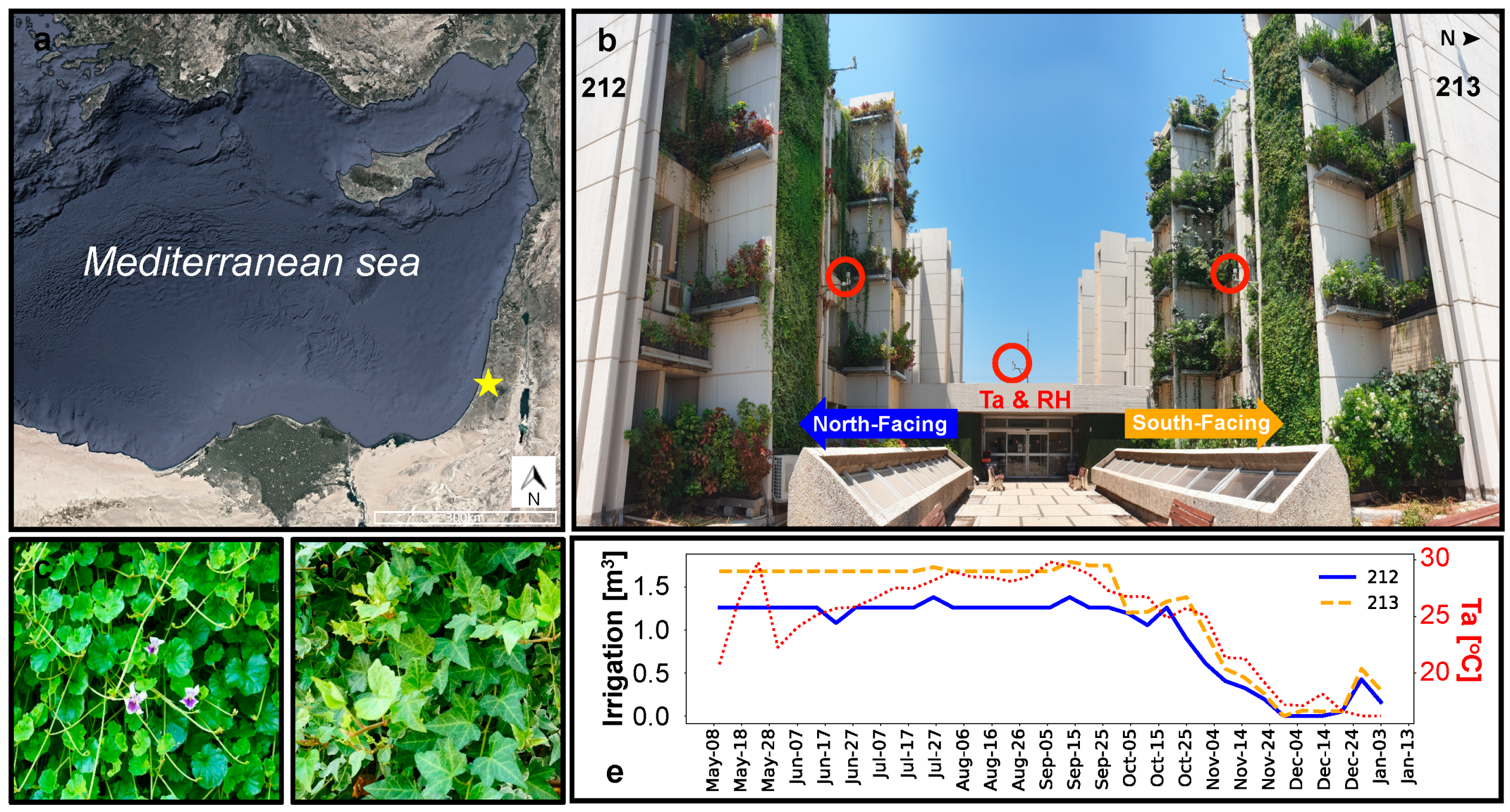
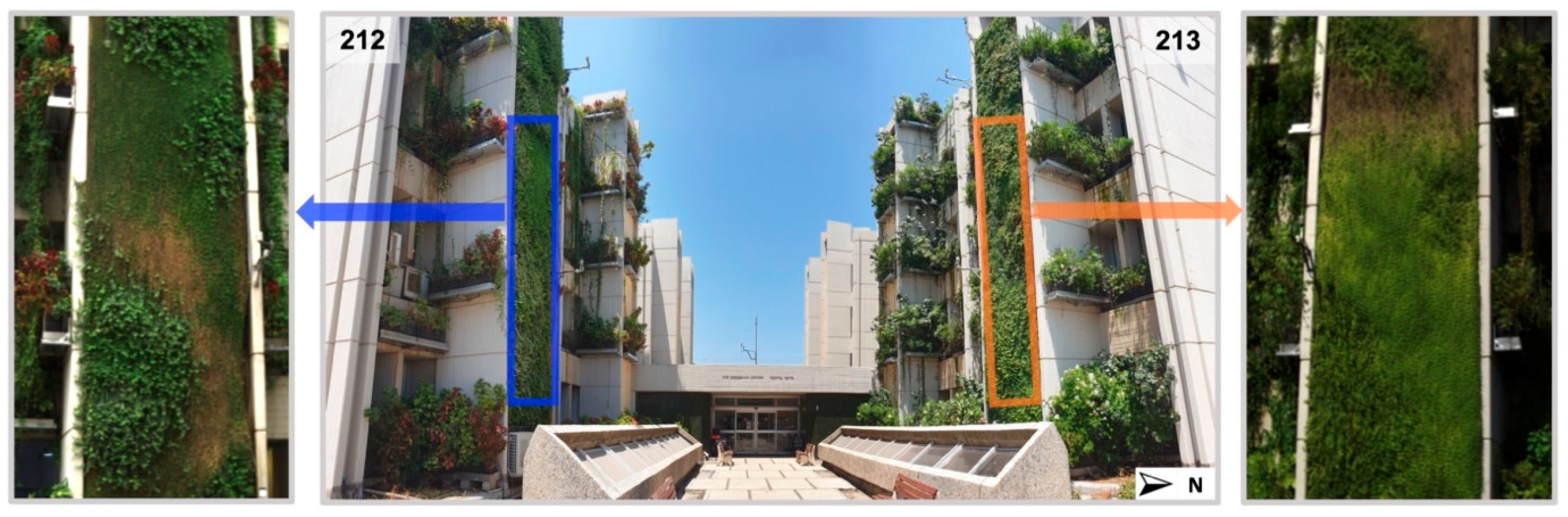
2.1. Study Area

The study was conducted on real-scale VGS as part of the BIU-VGS project at Bar Ilan University (32.067, 34.842) in Mediterranean climate Ramat Gan, the central region of Israel (Figure 1). The study site comprised three identical buildings in the southern campus, which replicated two east–west oriented street canyons. Each building consisted of five floors, with an overall height of 20 m. The canyons had concrete walls facing north and south. During the period from 3 to 18 November 2019, planters were installed on two parallel vertical walls in one of the canyons, covering approximately 450 m2 of vegetated area for each wall. Two VGS technologies were utilized—a green/living wall (GW) on the eastern shafts and a vertical forest (planter boxes attached to the wall) on the remaining walls and the western shafts. The GW was constructed using plastic modules containing a blended soil substrate for planting (40% peat, 40% coconut, and 20% perlite). The case study focused on the GWs located on two vertical concrete walls—one facing north (building 212) and the other facing south (building 213), as shown in Figure 1b. Each GW had dimensions of 11 m in height and 2.7 m in width, covered with plant species Viola hederacea (Figure 1c) and Hedera helix (Figure 1d).
The irrigation and fertilization of the GW were provided through an automated system based on scheduled programs planned by an irrigation expert. Each GW contained six irrigation lines, with drippers placed every 15 cm along the width of each line. Irrigation was applied at midnight either every one day (during summer) or every two days (during winter). Figure 1e presents the weekly average water accumulation during the study period. The quantities were adjusted based on seasonal variations and, in rare instances, an expert made decisions to decrease or increase water amounts based on direct observations made on-site. The average weekly quantities during May–October were 1.18 m3 (north-facing GW) and 1.56 m3 (south-facing GW), while irrigation significantly decreased during November–December to weekly average quantities of 0.16 m3 (north-facing) and 0.23 m3 (south-facing).

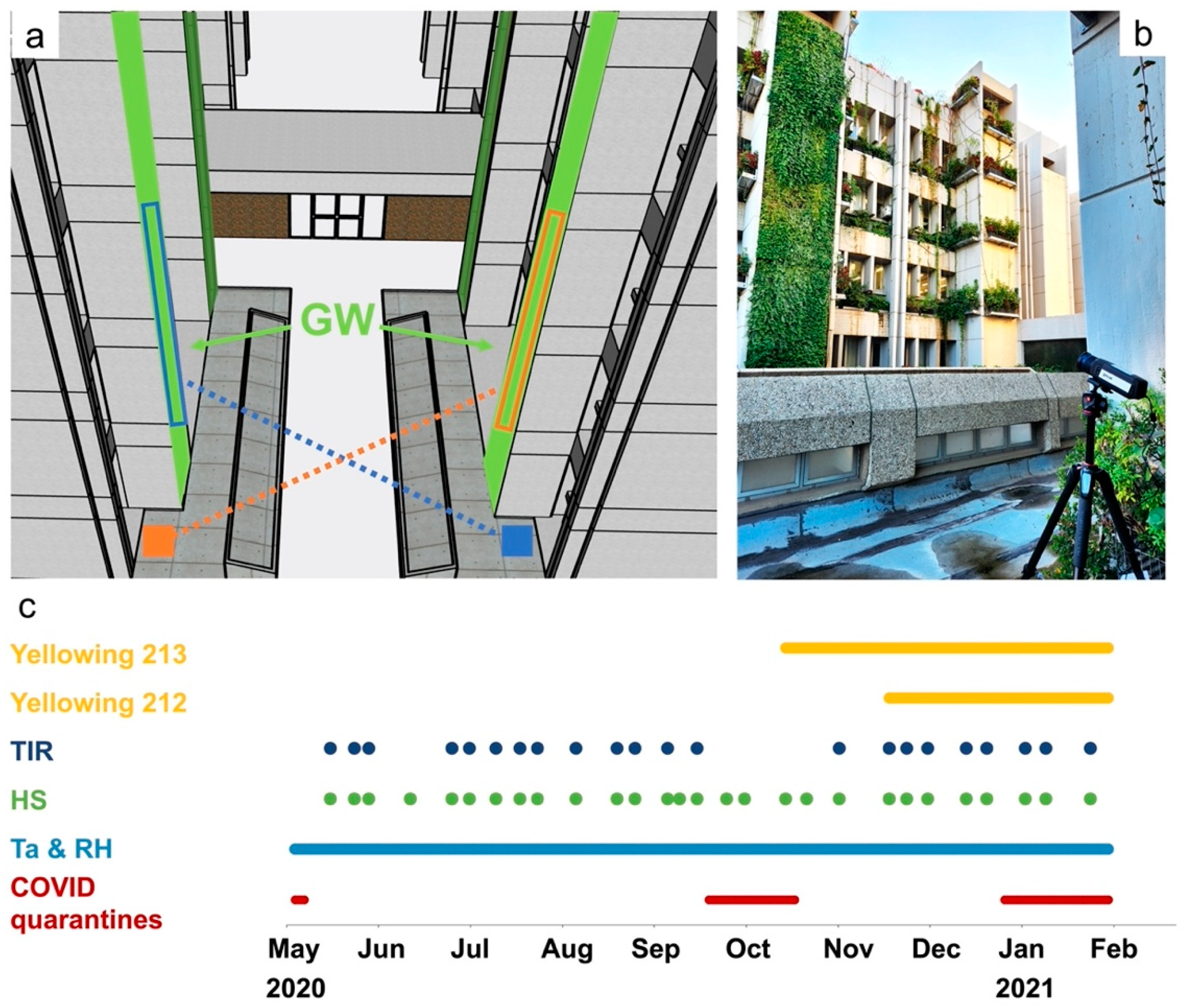
2.2. Data Acquisition

This study was conducted over 8 months between May and December 2020. GWs were monitored every 1–3 weeks using HS and TIR cameras. The cameras were mounted on a 1.5 m height tripod and manually operated from a fixed point on the ground, approximately 15 m away from the GW (Figure 2a,b). All images were collected during midday (11:00 A.M.–2:00 P.M. LT) under clear sky conditions.
The HS images were obtained using a Specim IQ® camera (Specim–Spectral Imaging, Oulu, Finland) with a spectral resolution of 7 nm and 204 bands across the wavelength range of 397–1003 nm. Each image from the Specim IQ® camera was a square of 512 × 512 pixels with a field of view (FOV) of 31°, providing a spatial resolution of 3 cm/pixel at the GW. All images were normalized using a 99% barium sulfate white reference (provided with the camera). Due to the vertical alignment, large scale, and limited accessibility of the VGS, the camera operated in “custom” mode, where the white reference was recorded and saved to the camera before the actual VGS recordings. The white reference was placed at the lower area of each GW and recorded every 15 min.
A FLIR A655sc (FLIR Systems, Wilsonville, OR, USA) camera was used for collecting TIR images. This camera is an uncooled microbolometer with 640 × 480 pixels, sensitive to radiation in the range of 7.5–14.0 µm. It is equipped with a lens with a FOV of 45° and provides a spatial resolution of 4 cm/pixel at the GW. The camera has a noise equivalent temperature difference (NETD, i.e., thermal sensitivity) of less than 30 mK and a thermal accuracy of ±2 °C or ±2% of the reading. The temperature values acquired by the camera were adjusted using FLIR Research IR software (version 4.40.9.30) by setting the air temperature (Ta), relative humidity (RH), and target distance. An emissivity of 0.95 was used to correct all thermal images. Due to technical issues with the thermal camera during COVID-19 quarantine restrictions, intermittent gaps occurred in the TIR time series data. Ta and RH were measured at 30 min intervals using HMP 155 Vaisala sensors with an accuracy of ±0.2 °C for Ta and ±1% for RH. These measurements were stored in cloud-based storage. Sensors were placed in three locations: 10 m from the GWs in the middle of the street canyon and 1 m near each GW (see red circles in Figure 1b). The timing of the data collection during this study is presented in Figure 2c.

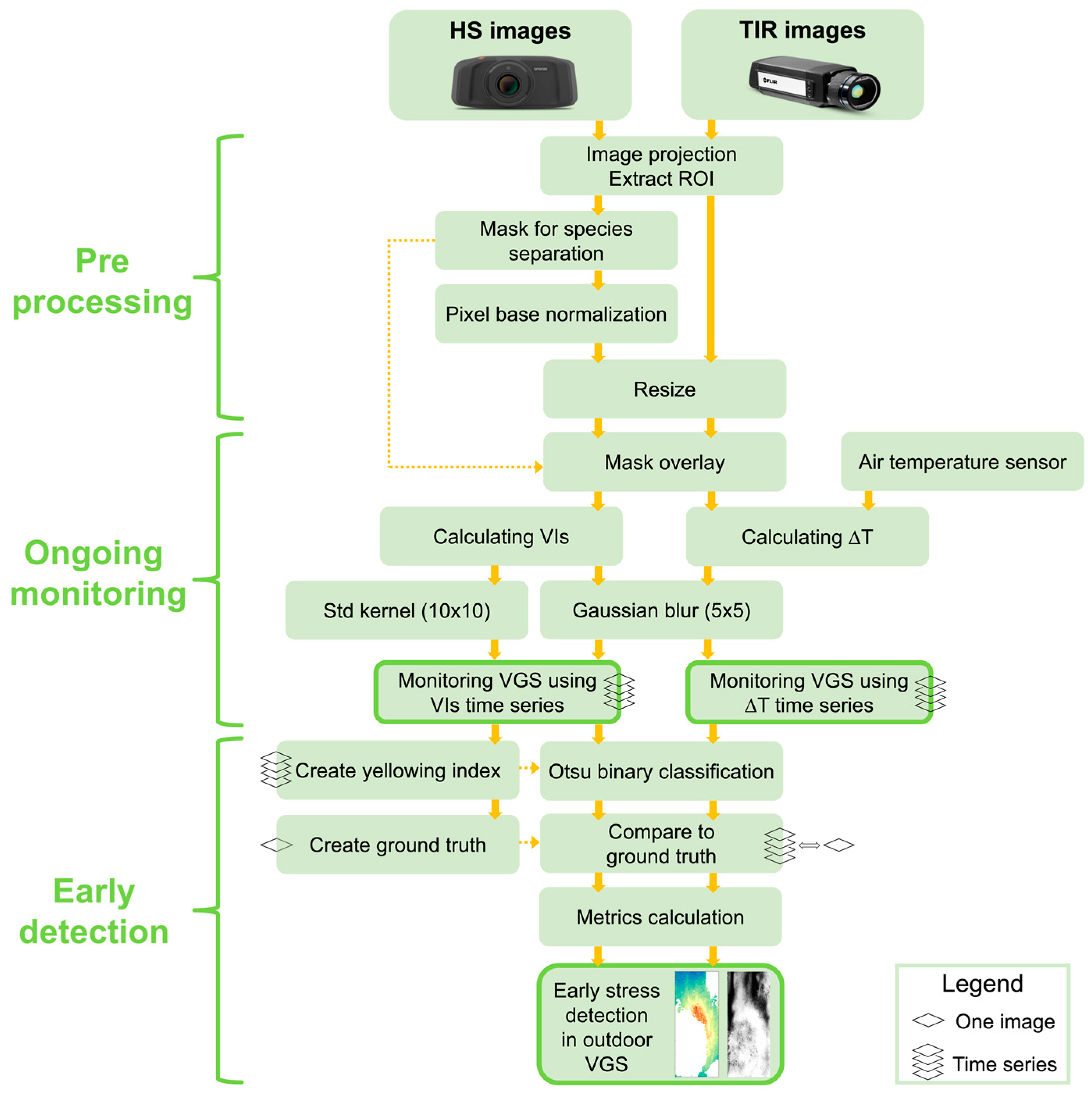
2.3. Image Processing

Figure 3 illustrates the image processing stages. The pre-processing of HS and TIR images involved their projection to each other using ArcGIS Pro software (version 3.0) and the extraction of Regions of Interest (ROIs) of approximately 13.5 m2 using the raster clip tool. The two plant species in the GW were separated (classified) due to their different phenological cycles, canopy closure characteristics, and vegetative properties. We employed the spectral angle mapper (SAM) supervised classification in ENVI software (version 5.6.1) to create a species mask for each GW (Figure 4). An image with a full green cover and without visible stress symptoms was selected for this purpose (north-facing: 14 September; south-facing: 24 August). Later, this mask was utilized to separate species in the HS and TIR time series analysis. After these pre-processing stages, the image processing flow was carried out using Python. The HS images were normalized (as described in Section 2.3.1), and all images (HS and TIR) were resized based on the smallest pixel found in each orientation time series.

2.3.1. Hyperspectral (HS) Image Processing

In the HS images, the white reference was positioned at the lower part of the GW. To eliminate illumination differences along the GW, a pixel-based spectrum normalization (sometimes referred to as Norm-1) was performed as follows:
R ^ i p = R i p / j = 1 204 R j p
where p is the pixel, and i and j are the bands. In the normalization process, each spectral band of a pixel is divided by the sum of all the pixel’s spectral bands, ensuring that the sum of all bands for a given pixel is equal to 1. This allows for relative comparisons and analysis of spectral information for the entire image, considering the proportion of each spectral band within a pixel.
For each species, 12 vegetation indices (VIs) were calculated, as shown in Table 1. The VIs were organized into categories based on their sensitivity (pigment; leaf structure; water content) and their band’s range (VIS-RGB; VIS-HS; NIR + VIS; NIR). For further analysis, two separate branches were pursued. (a) In the first branch, a kernel technique was employed. For each VI image, the standard deviation (“STD kernel”) was computed within 10 × 10 pixels moving window. This process involved iterating over the entire image, extracting data from each window, and generating a time series of the average STD kernel values for all VIs separated into species. These time series were used for the ongoing monitoring of the GWs. (b) In the second branch, a time series of VIs was built. For noise reduction in each VI image, Gaussian Blurring (size of 5 × 5 pixels) was applied. This is a smoothing method that removes noise generated by Gaussian distribution [44]. These time series presented the average value for each VI, separated into species, and were used for the ongoing monitoring of the GWs and later to examine the potential of early detection of vegetation stress in VGS (see Section 2.4).

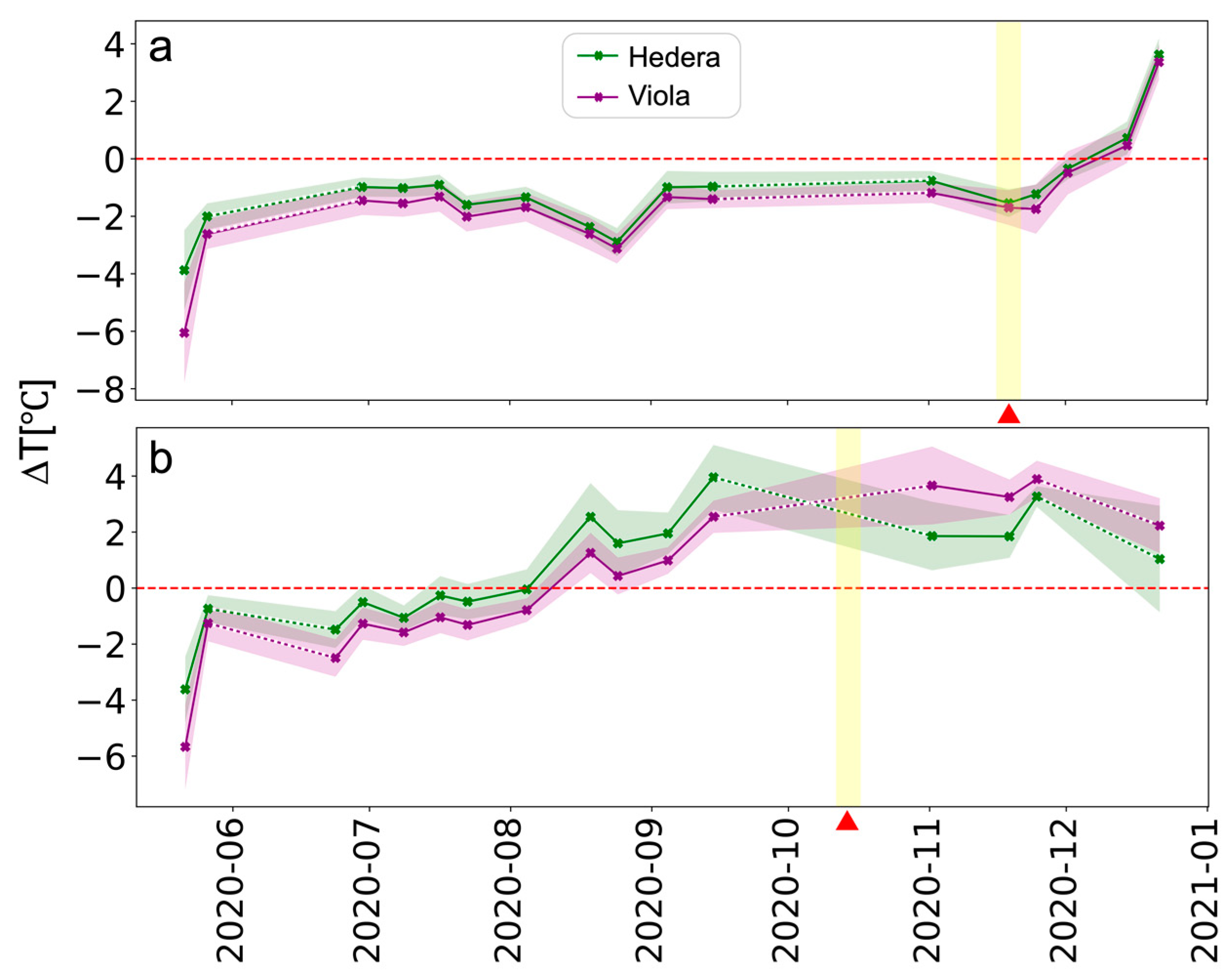
2.3.2. Thermal (TIR) Images Processing

Water stress is known to be correlated with stomatal closure, resulting in reduced transpiration and elevated leaf temperatures above the ambient temperature [58,59]. The canopy-to-air temperature difference (∆T) is widely used as an indicator of plant health, heat stress tolerance, or drought stress in crops [60], and is calculated based on the TIR images as follows:
T = TcanopyTa
where Tcanopy is the temperature of vegetation at each pixel and Ta is the air temperature measured in situ, 1 m from each GW. Generally, if a plant has sufficient water, ∆T ≤ 0, whereas under water stress, ∆T > 0. Gaussian Blurring (5 × 5 pixels) was applied to the ∆T images to reduce noise, similar to what was done for the VIs images. The time series of ∆T were separated into species and used for the ongoing monitoring of the GWs and later for early detection of vegetation stress in VGS using TIR images.

2.4. Stress Detection

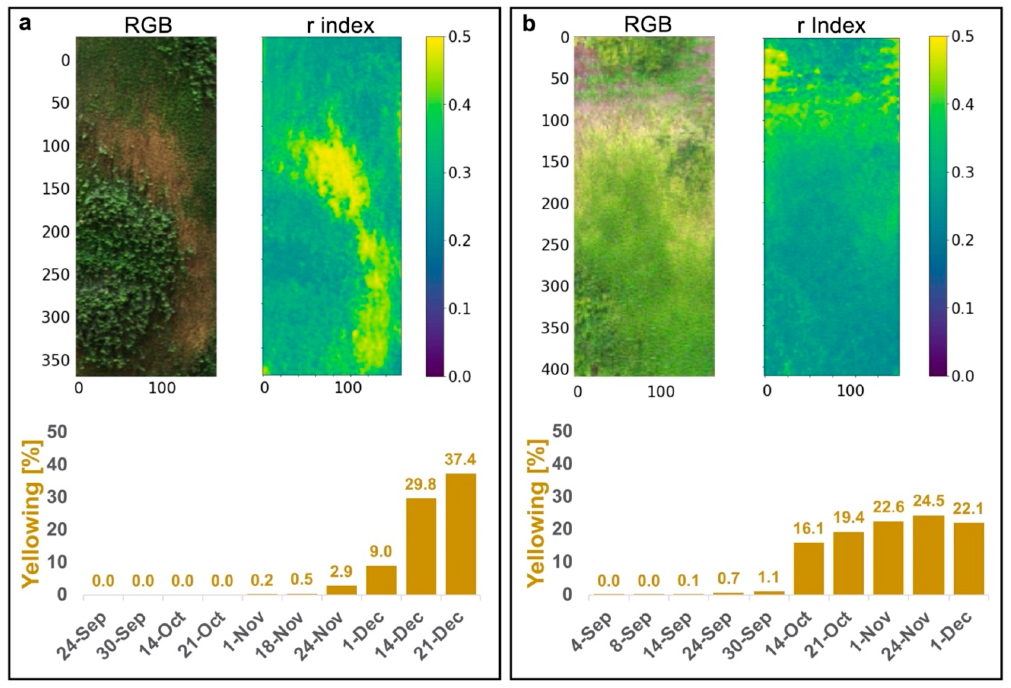
2.4.1. Yellowing Index and Ground Truth

In mid-October 2020 (south-facing GW—213) and mid-November 2020 (north-facing GW—212), the Viola hederacea plants along the GWs began to turn yellow and eventually died (Figure 5). In contrast, the Hedera helix plants, which are known as less sensitive plants, remained green and survived throughout the study and beyond. This period coincided with COVID-19 quarantine restrictions in Israel, and irrigation and fertilizer were not properly managed, likely contributing to vegetation degradation. The yellowing events caused significant damage to the GW, dissatisfaction among residents and passersby, and required extensive vegetation replacement using cranes. The time series of the Viola hederacea plants’ yellowing in both GWs are referred to as “yellowing events” in the study.
To investigate the usage of HS and TIR imaging for the early detection of stress events in the GWs, the yellowing areas in the time series were detected and delineated. A “yellowing index” for Viola hederacea was manually created to quantify the percentage of yellowing at each time step. This process involved visual observation of RGB and HS images, histogram investigation of yellow and green pixels, and examination of several RGB chlorophyll detection indices from the Sánchez-Sastre et al. [61] study (see Table A1 in Appendix A). The RGB r index (Table 1) was chosen to represent stressed vegetation. By setting a fixed threshold (based on histogram properties and visual inspection) of 0.3, the r index, hereafter referred to as the “yellowing index”, successfully captured yellow (r index value > 0.3) and green (r index value < 0.3) pixels. The yellowing index was analyzed for 10 time steps (from 24 September to 21 December at the north-facing GW and from 4 September to 1 December at the south-facing GW). One image per GW, close to the end of the yellowing event at each GW (14 December at the north-facing GW and 24 November at the south-facing GW), was selected as the reference image (ground truth) for stressed (yellow) pixels.

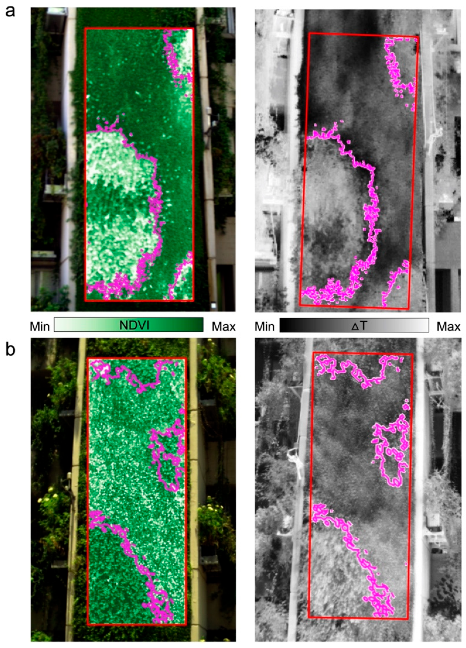
2.4.2. Stress Detection in VIs and Thermal Index Images

To investigate the feasibility of detecting stress events before the visual stage (yellowing) in VGS, we classified the HS VIs and ∆T thermal index images into stressed and green pixels. For each VI (Table 1) and thermal index image in the 10 yellowing index time steps, we used an unsupervised Otsu threshold [62] and Multi-Otsu [63] to divide each image into two or three groups based on the presence of yellow pixels. When minimal or no yellow pixels were detected in the image (yellowing index < 0.5%), the data was split into two groups. Conversely, when yellow pixels were already present in the image (the yellow index was greater than 0.5%), the data was divided into three groups to increase sensitivity and allow for early detection of pre-yellowed stressed pixels. Separating into two groups only allowed the differentiation of yellow pixels from other pixels but could not detect the variance (stressed, non-stressed) in the rest of the image. For each time step, we classified the pixels as green, stressed, and yellow (if present).

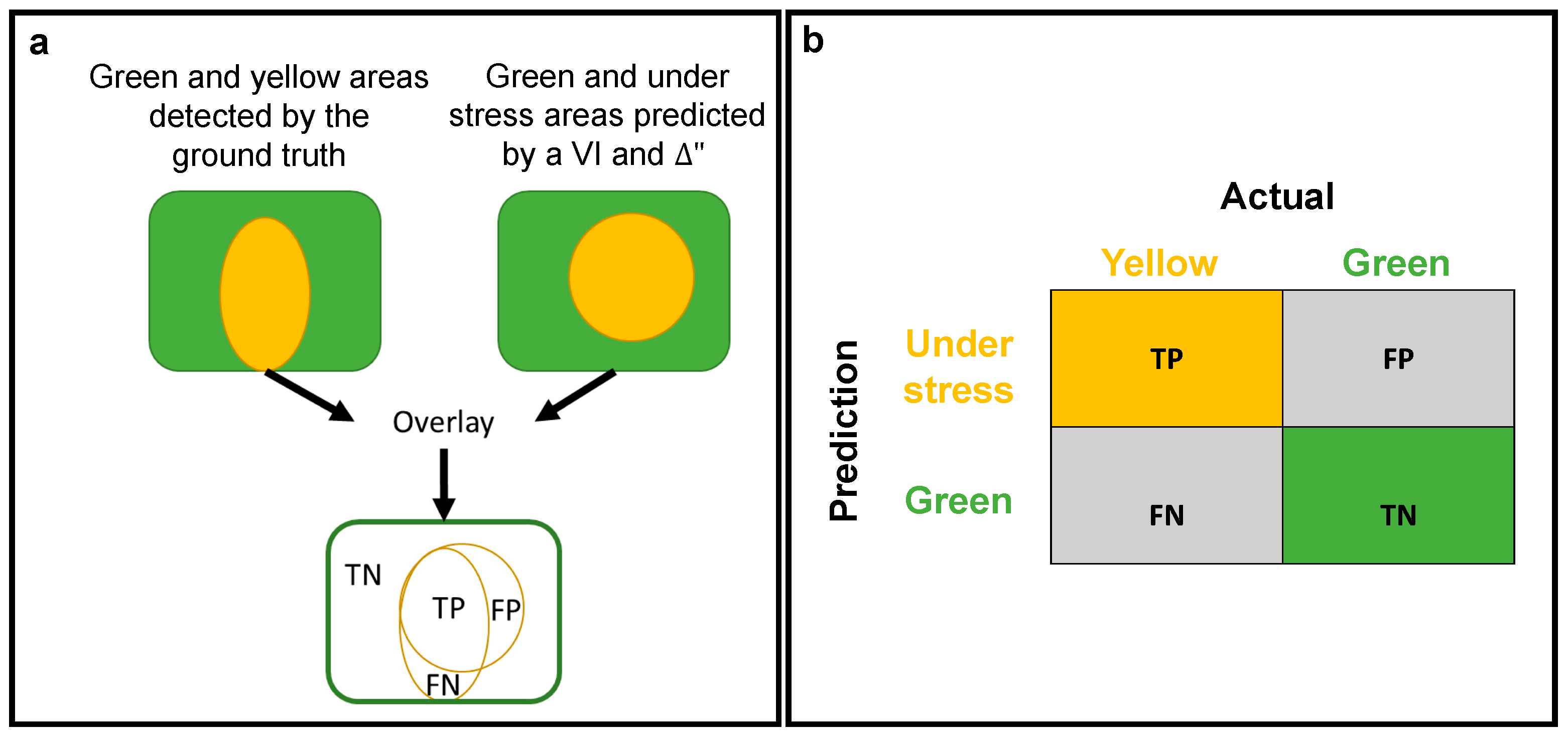
2.4.3. Stress Detection Performance Estimation

To evaluate the performance of the classifiers for early stress detection, we compared the classified (predicted: under stress or green) pixels from each HS VIs and ∆T index time step to the reference image (ground truth: yellow or green) and created a confusion matrix. The matrix was divided into four classes (Figure 6):
  • True positive (TP): yellow pixels that were correctly predicted as under stress.
  • False positive (FP): green pixels that were falsely predicted as under stress.
  • True negative (TN): green pixels that were correctly predicted as green.
  • False negative (FN): yellow pixels that were falsely predicted as green.
Figure 6. Illustrations of the confusion matrix structure as used in this study. (a) Process of the calculated area. (b) Confusion matrix for yellow (under stress) and green (healthy) pixels as recognized by the ground truth (actual) and the VIs and thermal indices (predicted).
Remotesensing 16 00302 g006
The metrics that were used to describe the classifiers’ success for early stress detection based on the confusion matrix were: accuracy, precision, false positive rate (false alarm), and F1 score. Recall was also calculated for the F1 score calculation. The metrics were calculated as follows:
Accuracy = (TP + TN)/(TP + FP + TN + FN)
Precision = TP/(TP + FP)
False positive rate (false alarm) = FP/(FP + TN)
Recall = TP/(TP + FN)
The F1 score, a single-value metric, combines precision and recall using the harmonic mean. It considers both false negatives and false positives, making it a useful metric for imbalanced data [64]. In this study, the F1 score was utilized to assess the classifier’s performance and ensure that the classification results were not merely due to random chance.

3. Results

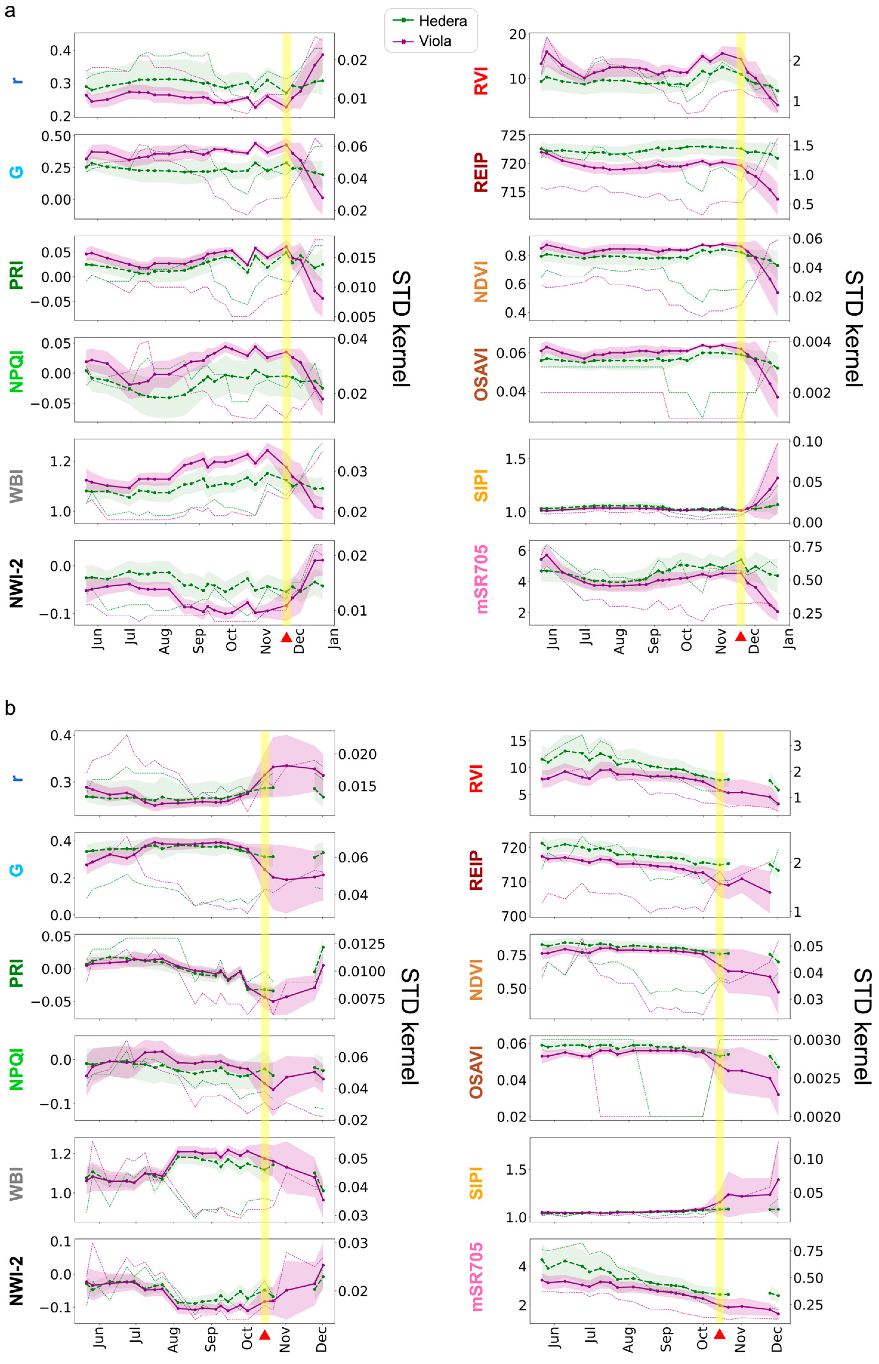
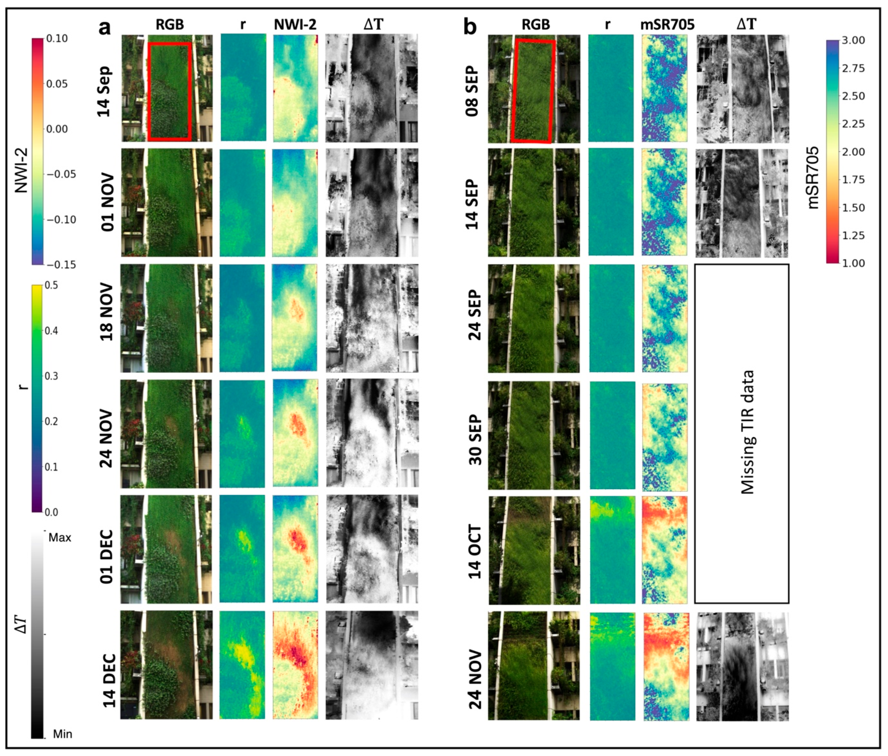
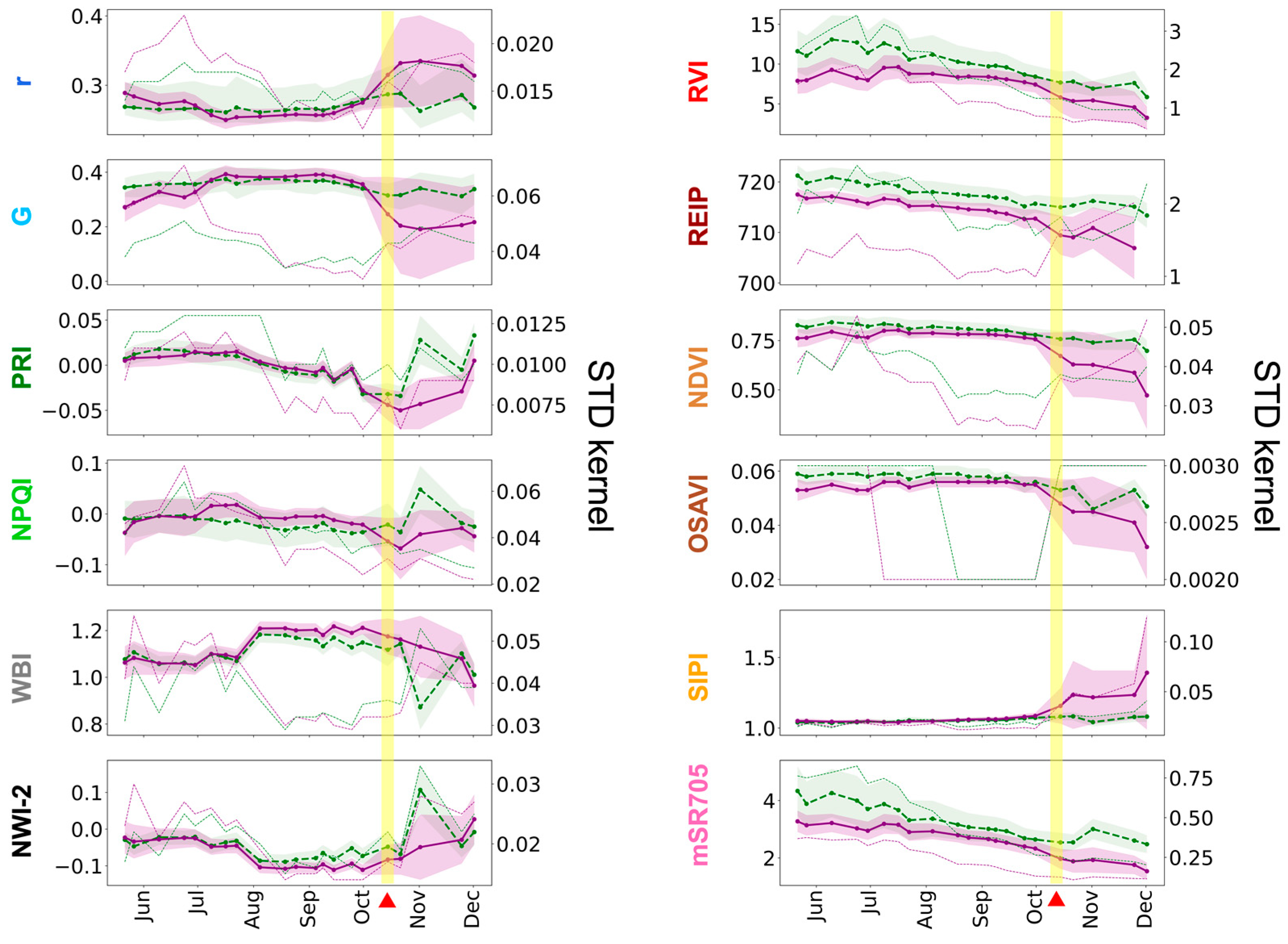
3.1. Ongoing Monitoring of VGS Using HS and TIR Images

The average value of VIs allowed us to assess the general status of vegetation in VGS using remote and non-destructive methods. Figure 7 shows the time series of average VIs values and STD kernel from May to December 2020 for the two species in each GW. In both GWs, the VIs initially showed stable or minor changes in average values for several months. However, as the yellow visual symptoms appeared on the plants, there were noticeable changes in vegetation dynamics, with some VIs showing a rise while others demonstrated a drop, as well as a rise in standard deviation and STD kernel, all synchronized with the yellowing event.
For the north-facing GW (Figure 7a), the average NDVI and standard deviation were 0.84 and 0.017 (Viola hederacea), and 0.79 and 0.019 (Hedera helix), respectively, from the beginning of the monitoring until the yellowing event. Just before the yellowing event (14 October to 1 November), the averages increased even further, and the standard deviation decreased (0.87, 0.009 for Viola hederacea; 0.83, 0.012 for Hedera helix). At the onset of the yellowing event (18 to 24 November), the averages decreased to 0.84 (−3.4% for Viola hederacea) and 0.81 (−2.4% for Hedera helix), and the standard deviation increased to 0.049 (540% for Viola hederacea) and 0.044 (360% for Hedera helix) compared to the period just before the yellowing event. As the yellowing event progressed (1 to 21 December), the averages further decreased to 0.651 (−22% for Viola hederacea) and 0.759 (−6% for Hedera helix), and the standard deviation increased to 0.154 (314% for Viola hederacea) and 0.077 (175% for Hedera helix), compared to the beginning of the yellowing event. Similarly, the REIP and OSAVI averages decreased, and the standard deviation increased at the beginning of the yellowing event and beyond. The water content indices, WBI and NW-2, exhibited periodic changes throughout the study, with more drastic average decreases and standard deviation increases (WBI: −5.7%, 270%; NW-2: −15.7%, 300%) in Viola hederacea at the beginning of the yellowing. Other VIs were either not stable (e.g., r, G, PRI, NPQI, RVI, and mSR705) or very stable (e.g., SIPI) throughout the seasons, but also showed a decrease in average value and a drastic increase in standard deviation at the beginning of the yellowing event. Both species experienced decreases in average VIs and increases in standard deviation, indicating degradation of the entire GW during the yellowing event. Nevertheless, the changes in average and standard deviation values were more significant for Viola hederacea, and it eventually turned yellow and died. As for the STD kernel, the increase for both species began even before the beginning of the yellowing event (around 21 October) and continued to rise until the end of the time series. Some indices (e.g., NDVI, G, and PRI) exhibited a more synchronized response with the vegetation condition than others (e.g., NPQI, NWI-2, and mSR705).
At the south-facing GW (Figure 7b), the NDVI averages and standard deviation were 0.77 and 0.013 (Viola hederacea), and 0.81 and 0.017 (Hedera helix) respectively from the beginning of the monitoring until the yellowing event, and 0.765 and 0.031 (Viola hederacea), and 0.788 and 0.032 (Hedera helix) just before the yellowing event (14 to 30 September). At the onset of the yellowing event (14 October), the average of both species dropped, and the standard deviation drastically increased by −12%, 387% (Viola hederacea), and −3.8%, 125% (Hedera helix) compared to the period just before the yellowing event. In this GW, the Viola hederacea yellowing event was much more intensive and was visually apparent from the beginning. Thus, the difference between the species is even more significant than in the north-facing GW. As the yellowing event progressed (21 October to 1 December), the averages continued to decrease to 0.578 (−14% for Viola hederacea) and 0.738 (−2.6% for Hedera helix). Several VIs (i.e., PRI, RVI, and mSR705) gradually decreased in both species throughout the monitoring period, which may indicate a gradual degradation in the entire GW vitality over the year. However, during the yellowing event, all VIs values sharply changed in average and standard deviation only for the Viola hederacea, which turned yellow, while Hedera helix changes were much more moderate. As for the STD kernel, the increase was more intense for Viola hederacea and started only at the beginning of the yellowing event (14 October) and continued to rise until the end of the time series. Like the north-facing GW, the STD kernels of the indices showed variable synchronization with the vegetation condition. However, unlike the north-facing GW, the STD kernel did not increase before the yellowing event.
During the study period, the north-facing GW remained entirely shaded, while the south-facing GW was fully exposed to sunlight during midday. Due to seasonal changes in the sun’s position, the south-facing GW (213) was entirely shaded in the last two images (24 November and 1 December), and partially shaded at the bottom of the GW (mainly at the Hedera helix areas) in the third image from the end (1 November). The shading conditions affected several pigment VIs in the last (2–3) images in the time series (Figure 7b). For example, PRI and NPQI sharply decreased during the yellowing event but started to increase on 1 November, even though the yellowing event continued. Due to the mixed sun-shadow conditions in the 1 November image, noisy values were observed in PRI, NPQI, WBI, and NW-2 in the Hedera helix dataset. Therefore, we excluded this time step from the time series. The complete time series data, including the excluded time step, can be found in Figure A1 in Appendix A.
Figure 8 presents the average ∆T of the two species for each GW. Data from the thermal camera is missing from 24 September until 21 October and on 23 June (north-facing GW) due to a technical problem (see Section 2.2). From the ∆T time series, it is evident that the north-facing GW (212) did not exhibit drastic changes in ∆T, except toward the end of the time series when ∆T began to rise as the GW yellowing progressed. This rise was observed in both species, although Hedera helix did not undergo yellowing. Conversely, at the south-facing GW, the ∆T index exhibited a consistent rise and was even slightly higher for the Hedera helix. Following the commencement of the yellowing event, ∆T in Viola hederacea continued to increase and surpassed that of Hedera helix. Data was unavailable before and after the commencement of the yellowing event, introducing uncertainty for this period. The consistent rise in ∆T was also observed in various HS VIs (see Figure 7b) and likely resulted from the gradual degradation of the entire GW. Eventually, this degradation led to the yellowing of Viola hederacea, whereas Hedera helix did not exhibit visual yellowing. The lowest ∆T in both GWs was recorded in the initial image (21 May), captured during a heatwave that transpired between 14–22 May 2020. During this period, the air temperature was elevated (Ta = 38 °C), and relative humidity was low (RH = 19.6%). In well-watered, unstressed vegetation, elevated air temperature, and reduced RH enhanced plant transpiration and resulted in decreased Tcanopy compared to air temperature (López et al., 2022 [65]).

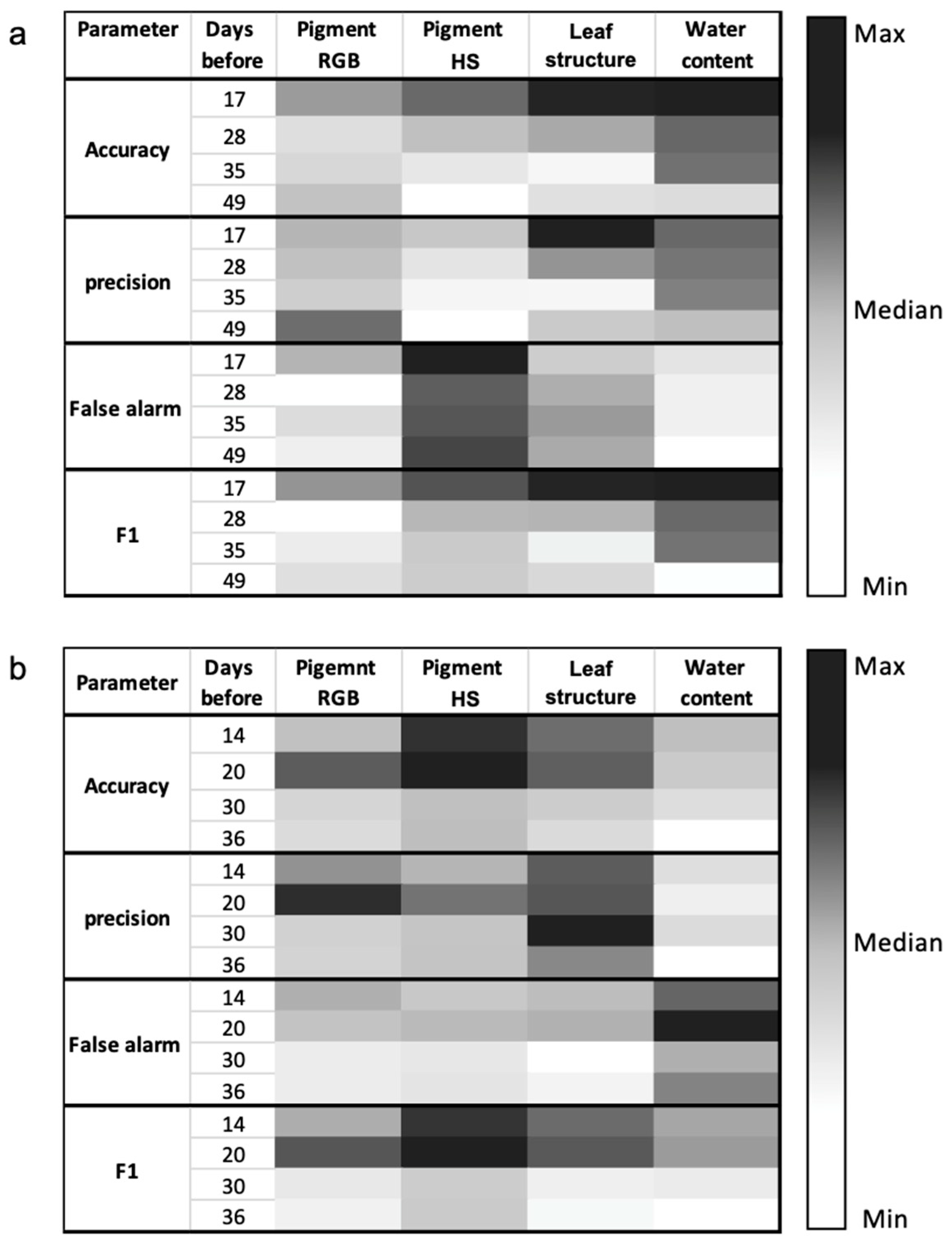
3.2. Early Detection of Stress Events

Figure 9 illustrates the use of the r index as the “ground truth” for desiccated vegetation. The RGB and the r index images are depicted for both GWs. The yellowing index [%] is computed based on the r > 0.3 threshold.
Following the binary classification of stressed/green pixels for each VI based on the Otsu threshold, each image was compared to the reference image at four time steps before the first yellowing was visually apparent. In total, 48 confusion matrices were computed (12 VIs × 4 time steps). Figure 10 shows a summary of the outcomes of the confusion matrices across the four VI categories outlined in Table 1 (RGB and HS pigment, leaf structure, and water content). At the north-facing GW (Figure 10a), 17 days before the onset of the yellowing event, metrics (accuracy, precision, and F1 score) displayed the highest values within the leaf structure and water content groups, both of which were derived from NIR wavelengths. In contrast, lower values were observed in the pigment groups (RGB and HS). Discrepancies in metrics among the classifiers became evident 35 days before the initial yellowing, occurring two months prior to the date of the ground-truth image, referenced for stressed vegetation (14 December). In the case of the south-facing GW (Figure 10b), distinguishing between classifiers proved more challenging, with the range between 14–20 days before the initial yellowing event appearing to be the inflection point, also approximately two months prior to the ground-truth image on 24 November. In this context, the HS pigment and leaf structure groups yielded the highest performance.
Table 2 outlines the highest metric scores within each VIs category during the final time step (17 days: north-facing; 14 days: south-facing) before the initial yellowing became visually apparent. At the north-facing GW, the water content index NWI-2 emerged as the most effective predictor (based on the F1 score), followed by the WBI index and then the OSAVI index. NWI-2 accurately predicted 85% of the yellowing area on 14 December as early as 1 November, with an accuracy of 0.91, precision of 0.84, false alarm rate of 0.06, and F1 score of 0.85. Similarly, NWI-2 anticipated 64% of the yellow pixels 35 days prior to the initial yellowing (approximately two months ahead of the reference yellowing image), achieving an accuracy of 0.85, precision of 0.82, false alarm rate of 0.06, and F1 score of 0.72. Meanwhile, at the south-facing GW, NPQI proved to be the strongest classifier, followed by the mSR705 and PRI indices. NPQI successfully predicted 72% of the 24 November yellow pixels as early as 30 September, boasting an accuracy of 0.87, precision of 0.73, false alarm rate of 0.08, and F1 score of 0.73.
Our investigation also encompassed the ∆T thermal index for the early detection of stressed vegetation. At the north-facing GW, the performance of ∆T on November 1 trailed behind the water content and leaf structure groups but surpassed the pigment group (accuracy of 0.87, precision of 0.77, false alarm rate of 0.09, and F1 score of 0.78). Previous time step metrics were slightly superior to the leaf structure group but still lagged behind the water content group. For the south-facing GW, missing data hindered our assessment of the time steps (24 and 30 September) that closely preceded the initial visible yellowing. Metrics for the final time step (14 September, around two and a half months before the reference image) were slightly lower than those of the other VIs groups (accuracy of 0.79, precision of 0.6, false alarm rate of 0.1, and F1 score of 0.53).
Figure 11 presents the time series of stress maps for both the north and south-facing GWs. In the north-facing GW, a small region within the ROI began to yellow on 18 November (Figure 11a). The yellowing, occurring in small portions a few meters above the ground, was nearly impossible to detect through visual investigation on site. This event’s origins can be traced back two weeks or more. On 14 September, thermal index imagery displayed cooler vegetation temperatures (denoted by darker hues) in certain areas, suggesting potential over-irrigation or drainage issues. By 1 November, these areas exhibited decreased water content (NWI-2). The initial yellowing transpired where vegetation temperatures were lower, indicating that the first affected regions suffered from excessive irrigation. Although irrigation was scaled back on 22 October (Figure 1e), the areas affected by over-irrigation failed to recover and were the first to exhibit yellowing.
At the south-facing GW (Figure 11b), owing to the absence of TIR image data (see Section 2.2), we were unable to pinpoint the cause of stress events. Nevertheless, stressed regions were successfully detected and visualized before the visible yellowing using VIs. The time series of PRI, NPQI, RVI, REIP, and mSR705 indices (Figure 7b) indicated a decline in plant vitality as early as August 2020. Thermal index images prior to the yellowing event (8 and 14 September) highlighted the warmest areas (represented by brighter tones) at the GW’s upper portion–these regions were the first to undergo yellowing on 14 October.

4. Discussion

Economic feasibility and maintenance are among the limiting factors of VGS [66]. While the significant construction costs are usually foreseen during the planning phase, clients often find themselves surprised by the unforeseen service costs linked to maintenance. The expense of irrigation is recognized as a significant factor [67], and the consequences of both inadequate and excessive irrigation, coupled with various abiotic or biotic stressors, can lead to VGS failure and necessitate extensive plant replacements [68]. While recommendations such as employing more tolerated plants [69,70] or irrigating using non-potable water [71] may alleviate certain operational costs, continuous monitoring of VGS is essential [20]. Real-time monitoring can identify stress indicators or system irregularities (e.g., drainage issues), allowing for timely intervention and averting the need for extensive plant replacements before irreversible damage occurs. This integrated approach not only addresses economic considerations but also underscores the importance of proactive monitoring in sustaining the long-term functionality and vitality of VGS.
In this study, we employed time series of hyperspectral (HS) and thermal infrared (TIR) imaging to illustrate practical approaches for the ongoing monitoring of green walls (GWs) (Figure 7 and Figure 8) and the early detection of stress events via unsupervised Otsu classification (Figure 10, Table 2). General statistics derived from vegetation indices (VIs) provided insights into the entire GW (Figure 7 and Figure 8). Additionally, mapping the VI images into stress maps (Figure 11) offered spatial information on vegetation and watering status—a highly valuable asset in VGS, given the constrained accessibility to plants and the substrate [72]. These insights provided information about the timing of stress and possible reasons, which could be associated with watering patterns (either lack or over-irrigation). Our analysis employed a semiautomated method, realized through Python code, for noninvasive continuous monitoring of GWs. Apart from the manual image capture process (Figure 2a,b), image projection, and pre-preparation of plant species masks, the entire image processing workflow (Figure 3) can be fully automated, providing valuable insights into VGS health. Notably, the manual aspects of this study carry some limitations. The image projection process could impact accuracy, and the consistent mask for species separation from a specific date might not precisely depict species boundaries in subsequent images due to vegetation growth. Nevertheless, vegetation growth remains restricted due to the small size of the GW modules.
In the continuous monitoring of both GWs, the yellowing event of Viola hederacea manifested as a decrease/increase in VIs values, a rise in standard deviation, and significant change in STD kernel across all VIs (Figure 7). In the north-facing GW, yellowing initially affected small sections, leading to a moderate decrease/increase in average VIs and a substantial upsurge in standard deviation and STD kernel values (Figure 7a). Hedera helix exhibited milder changes, potentially indicating a degree of stress without yellowing. Conversely, at the south-facing GW, the averages of several VIs consistently decreased/increased for both species since the summer, preceding the yellowing event, signifying the gradual deterioration of GW vitality over time (Figure 7b). Certain VIs were less sensitive and more stable over time (e.g., NDVI, SIPI), nevertheless, they were precise in detecting the yellowing event.
Increased vegetation variation is generally viewed as a marker of stress [73,74]. The pronounced escalation in standard deviation values across all VIs during the yellowing event, along with a rise in several VIs’ STD kernels even before the event’s onset, highlights plants’ varied responses to stress conditions. This gradual change during the yellowing event suggests that plants did not experience immediate yellowing but responded in a non-uniform manner. This indicates that these parameters can serve as stress detectors in VGS as well.
Some VIs were notably sensitive to shadow conditions, as observed in the final three images at the south-facing GW (Figure 7b and Figure A1 in Appendix A). Mixed shadow-sun conditions on 1 November also affected water content VIs, while several NIR-based VIs (such as RVI, NDVI, and SIPI) demonstrated lesser sensitivity to illumination changes, revealing the VIs’ trends. When devising a monitoring system utilizing image processing techniques in an outdoor environment, accounting for illumination variation along the VGS is crucial due to the vertical arrangement of the VGS and the intricate nature of the outdoor urban setting [75]. Although we employed pixel-based spectrum normalization to address illumination variation in the vertical direction (Section 2.3.1), we did not account for shadowed areas. Our findings emphasize that normalized NIR-based VIs, such as NDVI, maintain consistent patterns even under varying lighting conditions while still providing information regarding plant conditions. Based on these observations, we propose that such VIs could serve as valuable tools to mitigate the effects of diverse illumination and uphold reliable vegetation monitoring in nonuniformed illumination areas. Further exploration into shadow treatment in VGS and in other urban settings is warranted.
The time series of the ∆T index derived from TIR images provided supplementary insights into the plants’ water usage across the GWs (Figure 8). In the north-facing GW, a significant rise in the ∆T index was not observed until substantial sections of Viola hederacea along the GW displayed yellowing. Notably, the detection based on the ∆T time series lagged behind the HS VIs, where an increase was noted for both species only two weeks after the initiation of the yellowing event. This escalation in ∆T in the north-facing GW aligned with a sudden reduction in irrigation since 24 November (Figure 1e). Conversely, in the south-facing GW, ∆T increased progressively and remained elevated since the summer (August), extending through the yellowing event for both species. This pattern mirrored the HS VIs time series, indicating a gradual decline in the entire GW’s vitality over time (Figure 7b).
The VIs and ∆T index time series from both GWs reveal that while plant species’ index values may differ, the trends throughout the study were similar, suggesting stress across the entire GWs. Nonetheless, the plants’ response to stress varied: one species (Viola hederacea) turned yellow and ultimately perished, while the other (Hedera helix) remained green and survived. This distinction in species’ stress response was mirrored in the ongoing VI monitoring, with more pronounced changes observed in the affected species, particularly reflected in heightened variation (i.e., standard deviation and STD kernel). Given that a GW often contains multiple vegetation species along the wall, species separation might be necessary when designing a remote sensing image-based monitoring system for more precise and comprehensive monitoring. Nevertheless, monitoring without separation can still offer insights into the GW’s overall vitality and generate stress maps for spatial issue detection.
Early detection of stressed vegetation along the GWs was also explored in this study using RGB and HS VIs, as well as the ∆T thermal index, followed by Otsu unsupervised classification (Figure 10 and Table 2). Plant yellowing is a symptom of a spectrum of problems, such as watering issues, temperature stress, lack of sunlight, insufficient nutrition, over-fertilization, disease, and pests. Although the precise cause of vegetation yellowing was not systematically diagnosed in this study, we presented initial findings highlighting the early detection of vegetation yellowing. The assembled data, including HS and TIR images, irrigation patterns, and environmental conditions, yields promising outcomes for the early detection of issues in VGS. These results offer an initial step toward gaining valuable insights into the causes of stress. While stress detection techniques in agriculture have progressed with the advent of machine learning and deep learning, our preference was to employ more straightforward approaches using image thresholding. Thresholding methods continue to be applied in stress detection and segmentation process in recent agricultural studies [76,77,78]. Complex models demand extensive training datasets, particularly in our study’s context, where amassing substantial datasets of stress-affected pixels is undesirable in VGS. Additionally, the adoption of a simpler method establishes a baseline for future research in stress detection within VGS and presents an opportunity for further exploration as a practical tool.
As anticipated, the HS VIs outperformed the RGB VIs, yielding superior outcomes for the early detection of stressed areas. Performance varied among the VIs groups and GW orientations (north/south). In the north-facing GW, the water content and leaf structure VIs exhibited the most reliable predictive capability, while in the south-facing GW, the HS pigment and leaf structure indices demonstrated superior performance in predicting stressed areas. Thus, we recommend using multiple sets of VIs for comprehensive plant parameter monitoring in image-based monitoring. Notably, the leaf structure VIs group demonstrated high performance in both orientations.
Results from the north-facing GW revealed that 85% of stressed areas could be detected 17 days before visible yellowing (42 days before the ground-truth image) with an accuracy of 0.91. In the south-facing GW, 72% of the stressed area was detectable 14 days before visible yellowing (approximately two months before the ground-truth image), with an accuracy of 0.87. While early detection using ∆T in the north-facing GW exhibited lower performance compared to the water content and leaf structure VIs, it outperformed the pigment VIs group. In the south-facing GW, the performance of ∆T (alongside other VIs) was relatively diminished, likely due to data gaps and the limited time steps tested. Nonetheless, the visualization of the thermal index within stress maps (Figure 11) facilitated the identification of potential causes for vegetation stress.
HS vegetation indices were most effective in the early detection of stress; nevertheless, RGB vegetation indices, such as the r and G indices, are effective for real-time stress detection indicated by color changes. Unlike the costly HS camera used in this study, RGB VIs can readily detect pigment alterations through simple manual or automated thresholding processes (Figure 9 and Figure 10). Developing an alert system for VGS based on RGB camera technology is feasible and could serve as an ongoing control system for large-scale VGS operations. Note that in this study we employed narrow RGB channels extracted from the HS camera. This likely resulted in higher accuracy compared to the use of broader channels commonly found in low-cost RGB cameras.
Visualizing the HS VIs and thermal index through images (Figure 11) in conjunction with the irrigation patterns (Figure 1e) allowed us to pinpoint the cause of the plants’ stress in the north-facing GW. It is plausible that the yellowing event commenced in over-irrigated regions that were suddenly subjected to reduced irrigation. In the south-facing GW, although early yellowing occurrences were successfully detected, discerning the exact cause of plant stress proved challenging. An analysis of multiple indices’ time series from the south-facing GW (Figure 7b), including the thermal index (Figure 8b), revealed that the gradual decline in vegetation vitality commenced during the summer (August 2020), a full two months prior to the initial visual appearance of yellowing. Continuous irrigation over several months (from May to October) without adjustments to account for higher temperatures during the heatwave (14–22 May) and the summer months (July–August) (Figure 1e) likely initiated early plant stress. Moreover, the reduction in irrigation levels during October possibly exacerbated plant stress, ultimately culminating in the emergence of the yellowing event two weeks later.
Monitoring large-scale outdoor VGS with cameras is mainly a challenging task due to their vertical orientation limiting the accessibility needed for optimal camera position. To tackle the maintenance issues associated with vertical structures, robotics solutions like cable-driven and rail track robots have been developed [14,34,79]. Researchers have also explored various image-based monitoring approaches for vertical crops like greenhouse tomatoes, using multiple cameras positioned at different heights [80], as well as the use of mobile robots [81,82]. In the context of the ongoing monitoring of large-scale VGS health, it is essential to collect spatial data that enables the early detection of problems. Achieving this is challenging with the methods mentioned above. Additionally, outdoor VGS typically do not yield the same commercial profits as agricultural structures, necessitating the search for simpler and more practical monitoring solutions than those previously discussed. Implementing ground-based monitoring, as conducted in this study, by stationing cameras in a fixed position on the ground, offers a straightforward approach to continuous surveillance. Although the normalization of spectral data facilitated data analysis, it is important to acknowledge that the vertical orientation in real-scale VGS could potentially influence the results. Nonetheless, the findings from ongoing monitoring, the early detection of stressed vegetation, and the visualization of stress maps, as demonstrated in this study, indicate the feasibility of this method for the broad-scale monitoring of large-scale VGS at the single image (without mosaicking). Alternative solutions, such as utilizing multiple camera positions or employing adjustable mounts or tracks positioned in front of the VGS, should be considered to mitigate the vertical impact while preserving spatial distribution.
While our study presented the benefits of using precision agriculture methodologies in VGS, here we address certain limitations. The manual monitoring of specific ROI using expensive equipment (HS and TIR cameras) in our study raises concerns about the cost-effectiveness of continuously monitoring VGS. To optimize ongoing monitoring, it is crucial to explore alternative approaches, such as using more affordable sensors and implementing fully automated operations that can cover large-scale VGS. Additionally, shaded areas, common in VGS due to their vertical structure, need further study to find treatment solutions when employing image-based monitoring techniques. Technical issues with the TIR camera unveiled temporal gaps in the time series, hindering our ability to draw conclusive findings for the south-facing VGS. Furthermore, our study focused on the symptom of ‘yellowing’ without delving into the underlying causes of stress. Unexplored factors like nutrition, lighting conditions, and insect-related stresses may introduce complexities not addressed in our analysis. To address these limitations, future research should investigate the causes of stress in VGS, providing a more comprehensive understanding of the underlying phenomena.

5. Summary and Conclusions

The goal of this study was to examine the applicability of ground-based remote sensing techniques to monitor outdoor VGS. Additionally, we showcased a semiautomated approach for the early detection of vegetation stress and the visualization of spatially related issues through time series representation. The main conclusions of our study are as follows:
  • Consistent monitoring utilizing HS and TIR images can identify shifts in VGS health through index values, standard deviation, and STD kernel metrics.
  • Both vegetation species experienced stress, yet only Viola hederacea exhibited yellowing and eventual demise. Our observations suggest that the Hedera helix is less vulnerable to changes in irrigation patterns and can recover more effectively following stress events.
  • Species differentiation is pivotal for meticulous monitoring, accounting for each species’ unique characteristics and stress responses. Nevertheless, monitoring and visualizing the overall GW over time, without segregating individual species, can offer invaluable insights into the overall health of the GW and facilitate the identification of spatially linked issues.
  • Given the complexity of urban settings and the vertical arrangement of vegetation, variations in illumination should be considered when implementing image-based VGS monitoring, and further investigation is needed.
  • Early detection performance of stressed vegetation ranged from 14 to 35 days before visible yellowing, with an accuracy of 0.85 to 0.91.
  • The insights gained from this study could be harnessed to formulate an automated spatial decision support system that fosters more efficient VGS operations.
  • Additional investigations into stress detection methods and the adoption of low-cost cameras in outdoor VGS should be explored under different conditions and with various plant species.

Author Contributions

Conceptualization, N.Z., Y.C., V.A. and I.M.L.; data curation, N.Z.; formal analysis, N.Z.; funding acquisition, I.M.L.; investigation, N.Z.; methodology, N.Z., Y.C., V.A. and I.M.L.; project administration, I.M.L.; resources, I.M.L.; software, N.Z.; supervision, I.M.L.; validation, N.Z.; visualization, N.Z.; writing—original draft, N.Z.; writing—review and editing, N.Z., Y.C., V.A. and I.M.L. All authors have read and agreed to the published version of the manuscript.

Funding

The BIU-VGS project was funded by the Israel Ministry of Science and Technology (China-Israel cooperative scientific research 3-15706). The BIU-VGS project also received funding for the construction of the VGS and the monitoring equipment from the Israel Science Foundation institutional equipment grant (2320/18) and Bar-Ilan University (matching).

Data Availability Statement

The data presented in this study are available on request from the corresponding author. The data will be publicly available in the future as a separate publication.

Acknowledgments

The authors thank Amit Blizer for helping with the collection of images. N.Z. is a Ph.D. student partly supported by the BIU president scholarship for excellent Ph.D. students, the KKL-JNF scholarship, and the BIU-DSI scholarship.

Conflicts of Interest

The authors declare no conflicts of interest. The funders had no role in the design of the study; in the collection, analyses, or interpretation of data; in the writing of the manuscript; or in the decision to publish the results.

Appendix A

Table A1. RGB chlorophyll detection indices that examined for detecting yellow vegetation for preparation of the “yellowing index”.
RGB IndexDefinitionReference
r R/(R + G + B) [45]
g G/(R + G + B) [45]
b B/(R + G + B) [45]
R − G [45]
R − B [45]
G − B [45]
(R − G)/(R + G) [45,46]
(R − B)/(R + B) [45]
(G − B)/(G + B) [45]
(R − G)/(R + G + B) [45,83]
(R − B)/(R + G + B) [45]
(G − B)/(R + G + B) [45,83]
RGRI R/G [84]
GLI (2G − R − B)/(2G + R + B) [85]
Figure A1. As shown in Figure 7b only with 1 November which was excluded due to mixed sun-shadow conditions of the Hedera helix species in the south-facing GW.
Remotesensing 16 00302 g0a1

References

  1. Pérez, G.; Perini, K. Nature Based Strategies for Urban and Building Sustainability; Elsevier: Oxford/Cambridge, UK, 2018; ISBN 978-0-12-812150-4. [Google Scholar]
  2. Ghazalli, A.J.; Brack, C.; Bai, X.; Said, I. Physical and Non-Physical Benefits of Vertical Greenery Systems: A Review. J. Urban Technol. 2019, 26, 53–78. [Google Scholar] [CrossRef]
  3. Ottelé, M.; Van Bohemen, H.D.; Fraaij, A.L.A. Quantifying the Deposition of Particulate Matter on Climber Vegetation on Living Walls. Ecol. Eng. 2010, 36, 154–162. [Google Scholar] [CrossRef]
  4. Sternberg, T.; Viles, H.; Cathersides, A.; Edwards, M. Dust Particulate Absorption by Ivy (Hedera helix L) on Historic Walls in Urban Environments. Sci. Total Environ. 2010, 409, 162–168. [Google Scholar] [CrossRef]
  5. Susorova, I.; Azimi, P.; Stephens, B. The Effects of Climbing Vegetation on the Local Microclimate, Thermal Performance, and Air Infiltration of Four Building Facade Orientations. Build. Environ. 2014, 76, 113–124. [Google Scholar] [CrossRef]
  6. Zuckerman, N.; Lensky, I.M. Thermal Performance of Vertical Greenery Systems (VGS) in a Street Canyon: A Real-Scale Long-Term Experiment. Build. Environ. 2023, 244, 110750. [Google Scholar] [CrossRef]
  7. Coma, J.; Pérez, G.; De Gracia, A.; Burés, S.; Urrestarazu, M.; Cabeza, L.F. Vertical Greenery Systems for Energy Savings in Buildings: A Comparative Study between Green Walls and Green Facades. Build. Environ. 2017, 111, 228–237. [Google Scholar] [CrossRef]
  8. Wong, I.; Baldwin, A.N. Investigating the Potential of Applying Vertical Green Walls to High-Rise Residential Buildings for Energy-Saving in Sub-Tropical Region. Build. Environ. 2016, 97, 34–39. [Google Scholar] [CrossRef]
  9. Pérez, G.; Coma, J.; Barreneche, C.; De Gracia, A.; Urrestarazu, M.; Burés, S.; Cabeza, L.F. Acoustic Insulation Capacity of Vertical Greenery Systems for Buildings. Appl. Acoust. 2016, 110, 218–226. [Google Scholar] [CrossRef]
  10. Paull, N.; Krix, D.; Torpy, F.; Irga, P. Can Green Walls Reduce Outdoor Ambient Particulate Matter, Noise Pollution and Temperature? Int. J. Environ. Res. Public Health 2020, 17, 5084. [Google Scholar] [CrossRef]
  11. Chan, S.H.M.; Qiu, L.; Esposito, G.; Mai, K.P. Vertical Greenery Buffers against Stress: Evidence from Psychophysiological Responses in Virtual Reality. Landsc. Urban Plan. 2021, 213, 104127. [Google Scholar] [CrossRef]
  12. Fonseca, F.; Paschoalino, M.; Silva, L. Health and Well-Being Benefits of Outdoor and Indoor Vertical Greening Systems: A Review. Sustainability 2023, 15, 4107. [Google Scholar] [CrossRef]
  13. Huang, Z.; Lu, Y.; Wong, N.H.; Poh, C.H. The True Cost of “Greening” a Building: Life Cycle Cost Analysis of Vertical Greenery Systems (VGS) in Tropical Climate. J. Clean. Prod. 2019, 228, 437–454. [Google Scholar] [CrossRef]
  14. Carmichael, M.; Khonasty, R.; Wilkinson, S.; Schork, T. The Wallbot: A Low-Cost Robot for Green WallInspection. In Proceedings of the Australasian Conference on Robotics and Automation 2020, Brisbane, Australia, 8–10 December 2020. [Google Scholar]
  15. Dahanayake, K.C.; Chow, C.L. Moisture Content, Ignitability, and Fire Risk of Vegetation in Vertical Greenery Systems. Fire Ecol. 2018, 14, 125–142. [Google Scholar] [CrossRef]
  16. Conejos, S.; Chew, M.Y.L.; Azril, F.H.B. Green Maintainability Assessment of High-Rise Vertical Greenery Systems. Facilities 2019, 37, 1008–1047. [Google Scholar] [CrossRef]
  17. Helman, D.; Yungstein, Y.; Mulero, G.; Michael, Y. High-Throughput Remote Sensing of Vertical Green Living Walls (VGWs) in Workplaces. Remote Sens. 2022, 14, 3485. [Google Scholar] [CrossRef]
  18. Valente De Macedo, L.S.; Barda Picavet, M.E.; Puppim De Oliveira, J.A.; Shih, W.-Y. Urban Green and Blue Infrastructure: A Critical Analysis of Research on Developing Countries. J. Clean. Prod. 2021, 313, 127898. [Google Scholar] [CrossRef]
  19. Segovia-Cardozo, D.A.; Rodríguez-Sinobas, L.; Zubelzu, S. Living Green Walls: Estimation of Water Requirements and Assessment of Irrigation Management. Urban For. Urban Green. 2019, 46, 126458. [Google Scholar] [CrossRef]
  20. Gunawardena, K.; Steemers, K. Urban Living Walls: Reporting on Maintenance Challenges from a Review of European Installations. Archit. Sci. Rev. 2020, 63, 526–535. [Google Scholar] [CrossRef]
  21. Mosa, K.A.; Ismail, A.; Helmy, M. Introduction to Plant Stresses. In Plant Stress Tolerance; SpringerBriefs in Systems Biology; Springer International Publishing: Cham, UK, 2017; pp. 1–19. ISBN 978-3-319-59377-7. [Google Scholar]
  22. Pallottino, F.; Antonucci, F.; Costa, C.; Bisaglia, C.; Figorilli, S.; Menesatti, P. Optoelectronic Proximal Sensing Vehicle-Mounted Technologies in Precision Agriculture: A Review. Comput. Electron. Agric. 2019, 162, 859–873. [Google Scholar] [CrossRef]
  23. Pande, C.B.; Moharir, K.N. Application of Hyperspectral Remote Sensing Role in Precision Farming and Sustainable Agriculture Under Climate Change: A Review. In Climate Change Impacts on Natural Resources, Ecosystems and Agricultural Systems; Pande, C.B., Moharir, K.N., Singh, S.K., Pham, Q.B., Elbeltagi, A., Eds.; Springer Climate; Springer International Publishing: Cham, UK, 2023; pp. 503–520. ISBN 978-3-031-19058-2. [Google Scholar]
  24. Verma, B.; Porwal, M.; Jha, A.K.; Vyshnavi, R.G.; Rajpoot, A.; Nagar, A.K. Enhancing Precision Agriculture and Environmental Monitoring Using Proximal Remote Sensing. JEAI 2023, 45, 162–176. [Google Scholar] [CrossRef]
  25. Barbedo, J. A Review on the Use of Unmanned Aerial Vehicles and Imaging Sensors for Monitoring and Assessing Plant Stresses. Drones 2019, 3, 40. [Google Scholar] [CrossRef]
  26. Lu, B.; Dao, P.; Liu, J.; He, Y.; Shang, J. Recent Advances of Hyperspectral Imaging Technology and Applications in Agriculture. Remote Sens. 2020, 12, 2659. [Google Scholar] [CrossRef]
  27. Thenkabail, P.S.; Lyon, J.G.; Huete, A. (Eds.) Hyperspectral Indices and Image Classifications for Agriculture and Vegetation: Hyperspectral Remote Sensing of Vegetation, 2nd ed.; CRC Press: Boca Raton, FL, USA, 2018; ISBN 978-1-315-15933-1. [Google Scholar]
  28. Zhang, J.; Huang, Y.; Pu, R.; Gonzalez-Moreno, P.; Yuan, L.; Wu, K.; Huang, W. Monitoring Plant Diseases and Pests through Remote Sensing Technology: A Review. Comput. Electron. Agric. 2019, 165, 104943. [Google Scholar] [CrossRef]
  29. Cohen, Y.; Alchanatis, V. Spectral and Spatial Methods for Hyperspectral and Thermal Image-Analysis to Estimate Biophysical and Biochemical Properties of Agricultural Crops. In Biophysical and Biochemical Characterization and Plant Species Studies; Thenkabail, P.S., Lyon, J.G., Huete, A., Eds.; CRC Press: Boca Raton, FL, USA, 2018; pp. 73–101. ISBN 978-0-429-43118-0. [Google Scholar]
  30. Cohen, Y.; Vellidis, G.; Campillo, C.; Liakos, V.; Graff, N.; Saranga, Y.; Snider, J.L.; Casadesús, J.; Millán, S.; Prieto, M.D.H. Applications of Sensing to Precision Irrigation. In Sensing Approaches for Precision Agriculture; Kerry, R., Escolà, A., Eds.; Progress in Precision Agriculture; Springer International Publishing: Cham, Switzerland, 2021; pp. 301–332. ISBN 978-3-030-78430-0. [Google Scholar]
  31. Katz, L.; Ben-Gal, A.; Litaor, M.I.; Naor, A.; Peres, M.; Bahat, I.; Netzer, Y.; Peeters, A.; Alchanatis, V.; Cohen, Y. Spatiotemporal Normalized Ratio Methodology to Evaluate the Impact of Field-Scale Variable Rate Application. Precis. Agric. 2022, 23, 1125–1152. [Google Scholar] [CrossRef]
  32. Katz, L.; Ben-Gal, A.; Litaor, M.I.; Naor, A.; Peres, M.; Peeters, A.; Alchanatis, V.; Cohen, Y. A Spatiotemporal Decision Support Protocol Based on Thermal Imagery for Variable Rate Drip Irrigation of a Peach Orchard. Irrig. Sci. 2023, 41, 215–233. [Google Scholar] [CrossRef]
  33. Halgamuge, M.N.; Bojovschi, A.; Fisher, P.M.J.; Le, T.C.; Adeloju, S.; Murphy, S. Internet of Things and Autonomous Control for Vertical Cultivation Walls towards Smart Food Growing: A Review. Urban For. Urban Green. 2021, 61, 127094. [Google Scholar] [CrossRef]
  34. Hoffmann, K.A.; Schröder, S.; Nehls, T.; Pitha, U.; Pucher, B.; Zluwa, I.; Gantar, D.; Erjavec, S.; Kozamernik, J. Vertical Green 2.0—The Good, the Bad and the Science; Universitätsverlag der TU Berlin: Berlin, Germany, 2023. [Google Scholar]
  35. Tasrif Anubhove, M.S.; Ashrafi, N.; Saleque, A.M.; Akter, M.; Saif, S.U. Machine Learning Algorithm Based Disease Detection in Tomato with Automated Image Telemetry for Vertical Farming. In Proceedings of the 2020 International Conference on Computational Performance Evaluation (ComPE), Shillong, India, 2–4 July 2020; pp. 250–254. [Google Scholar]
  36. Duman, S.; Elewi, A. Design of a Smart Vertical Farming System Using Image Processing. In Proceedings of the 2022 2nd International Conference on Computing and Machine Intelligence (ICMI), Istanbul, Turkey, 15 April 2022; pp. 1–5. [Google Scholar]
  37. Pérez-Urrestarazu, L.; Egea, G.; Franco-Salas, A.; Fernández-Cañero, R. Irrigation Systems Evaluation for Living Walls. J. Irrig. Drain Eng. 2014, 140, 04013024. [Google Scholar] [CrossRef]
  38. Pérez-Urrestarazu, L. Water Consumption of Felt-Based Outdoor Living Walls in Warm Climates. Urban For. Urban Green. 2021, 59, 127025. [Google Scholar] [CrossRef]
  39. Cameron, R.W.F.; Taylor, J.E.; Emmett, M.R. What’s ‘Cool’ in the World of Green Façades? How Plant Choice Influences the Cooling Properties of Green Walls. Build. Environ. 2014, 73, 198–207. [Google Scholar] [CrossRef]
  40. Yin, H.; Kong, F.; Middel, A.; Dronova, I.; Xu, H.; James, P. Cooling Effect of Direct Green Façades during Hot Summer Days: An Observational Study in Nanjing, China Using TIR and 3DPC Data. Build. Environ. 2017, 116, 195–206. [Google Scholar] [CrossRef]
  41. Piro, P.; Porti, M.; Veltri, S.; Lupo, E.; Moroni, M. Hyperspectral Monitoring of Green Roof Vegetation Health State in Sub-Mediterranean Climate: Preliminary Results. Sensors 2017, 17, 662. [Google Scholar] [CrossRef] [PubMed]
  42. Moroni, M.; Porti, M.; Piro, P. Design of a Remote-Controlled Platform for Green Roof Plants Monitoring via Hyperspectral Sensors. Water 2019, 11, 1368. [Google Scholar] [CrossRef]
  43. Yuan, X.; Laakso, K.; Davis, C.D.; Guzmán, Q.J.A.; Meng, Q.; Sanchez-Azofeifa, A. Monitoring the Water Stress of an Indoor Living Wall System Using the “Triangle Method”. Sensors 2020, 20, 3261. [Google Scholar] [CrossRef] [PubMed]
  44. Laganière, R. OpenCV Computer Vision Application Programming Cookbook Second Edition; Packt Publishing Ltd.: Birmingham, UK, 2014. [Google Scholar]
  45. Kawashima, S.; Nakatani, M. An Algorithm for Estimating Chlorophyll Content in Leaves Using a Video Camera. Ann. Bot. 1998, 81, 49–54. [Google Scholar] [CrossRef]
  46. Tucker, C.J. Red and Photographic Infrared Linear Combinations for Monitoring Vegetation. Remote Sens. Environ. 1979, 8, 127–150. [Google Scholar] [CrossRef]
  47. Gamon, J.A.; Peñuelas, J.; Field, C.B. A Narrow-Waveband Spectral Index That Tracks Diurnal Changes in Photosynthetic Efficiency. Remote Sens. Environ. 1992, 41, 35–44. [Google Scholar] [CrossRef]
  48. Penuelas, J.; Filella, I.; Gamon, J.A. Assessment of Photosynthetic Radiation-Use Efficiency with Spectral Reflectance. New Phytol. 1995, 131, 291–296. [Google Scholar] [CrossRef]
  49. Barnes, J.D.; Balaguer, L.; Manrique, E.; Elvira, S.; Davison, A.W. A Reappraisal of the Use of DMSO for the Extraction and Determination of Chlorophylls a and b in Lichens and Higher Plants. Environ. Exp. Bot. 1992, 32, 85–100. [Google Scholar] [CrossRef]
  50. Peñuelas, J.; Baret, F.; Filella, I. Semi-Empirical Indices to Assess Carotenoids/Chlorophyll Alpha Ratio from Leaf Spectral Reflectance. Photosynthetica 1995, 31, 221–230. [Google Scholar]
  51. Sims, D.A.; Gamon, J.A. Relationships between Leaf Pigment Content and Spectral Reflectance across a Wide Range of Species, Leaf Structures and Developmental Stages. Remote Sens. Environ. 2002, 81, 337–354. [Google Scholar] [CrossRef]
  52. Jordan, C.F. Derivation of Leaf-Area Index from Quality of Light on the Forest Floor. Ecology 1969, 50, 663–666. [Google Scholar] [CrossRef]
  53. Guyot, G.; Baret, F.; Major, D.J. High Spectral Resolution: Determination of Spectral Shifts between the Red and near Infrared. Int. Arch. Photogramm. Remote Sens. 1988, 11, 740–760. [Google Scholar]
  54. Rouse, J.W., Jr.; Haas, R.H.; Schell, J.A.; Deering, D.W. Monitoring Vegetation Systems in the Great Plains with Erts. NASA Spec. Publ. 1974, 351, 309. [Google Scholar]
  55. Rondeaux, G.; Steven, M.; Baret, F. Optimization of Soil-Adjusted Vegetation Indices. Remote Sens. Environ. 1996, 55, 95–107. [Google Scholar] [CrossRef]
  56. Penuelas, J.; Pinol, J.; Ogaya, R.; Filella, I. Estimation of Plant Water Concentration by the Reflectance Water Index WI (R900/R970). Int. J. Remote Sens. 1997, 18, 2869–2875. [Google Scholar] [CrossRef]
  57. Babar, M.A.; Reynolds, M.P.; Van Ginkel, M.; Klatt, A.R.; Raun, W.R.; Stone, M.L. Spectral Reflectance Indices as a Potential Indirect Selection Criteria for Wheat Yield under Irrigation. Crop. Sci. 2006, 46, 578–588. [Google Scholar] [CrossRef]
  58. Idso, S.B.; Jackson, R.D.; Reginato, R.J. Remote-Sensing of Crop Yields: Canopy Temperature and Albedo Measurements Have Been Quantitatively Correlated with Final Harvests of Wheat. Science 1977, 196, 19–25. [Google Scholar] [CrossRef]
  59. Jackson, R.D.; Reginato, R.J.; Idso, S.B. Wheat Canopy Temperature: A Practical Tool for Evaluating Water Requirements. Water Resour. Res. 1977, 13, 651–656. [Google Scholar] [CrossRef]
  60. Maes, W.H.; Steppe, K. Estimating Evapotranspiration and Drought Stress with Ground-Based Thermal Remote Sensing in Agriculture: A Review. J. Exp. Bot. 2012, 63, 4671–4712. [Google Scholar] [CrossRef]
  61. Sánchez-Sastre, L.F.; Alte Da Veiga, N.M.S.; Ruiz-Potosme, N.M.; Carrión-Prieto, P.; Marcos-Robles, J.L.; Navas-Gracia, L.M.; Martín-Ramos, P. Assessment of RGB Vegetation Indices to Estimate Chlorophyll Content in Sugar Beet Leaves in the Final Cultivation Stage. AgriEngineering 2020, 2, 128–149. [Google Scholar] [CrossRef]
  62. Otsu, N. A Threshold Selection Method from Gray-Level Histograms. IEEE Trans. Syst. Man Cybern. 1979, 9, 62–66. [Google Scholar] [CrossRef]
  63. Huang, D.Y.; Lin, T.W.; Hu, W.C. Automatic Multilevel Thresholding Based on Two-Stage Otsu’s Method with Cluster Determination by Valley Estimation. Int. J. Innov. Comput. Inf. Control. 2011, 7, 5631–5644. [Google Scholar]
  64. Korkmaz, S. Deep Learning-Based Imbalanced Data Classification for Drug Discovery. J. Chem. Inf. Model. 2020, 60, 4180–4190. [Google Scholar] [CrossRef] [PubMed]
  65. López, R.; Ramírez-Valiente, J.A.; Pita, P. How Plants Cope with Heatwaves in a Drier Environment. Flora 2022, 295, 152148. [Google Scholar] [CrossRef]
  66. Bustami, R.A.; Belusko, M.; Ward, J.; Beecham, S. Vertical Greenery Systems: A Systematic Review of Research Trends. Build. Environ. 2018, 146, 226–237. [Google Scholar] [CrossRef]
  67. Natarajan, M.; Rahimi, M.; Sen, S.; Mackenzie, N.; Imanbayev, Y. Living Wall Systems: Evaluating Life-Cycle Energy, Water and Carbon Impacts. Urban Ecosyst. 2015, 18, 1–11. [Google Scholar] [CrossRef]
  68. Riley, B. The State of the Art of Living Walls: Lessons Learned. Build. Environ. 2017, 114, 219–232. [Google Scholar] [CrossRef]
  69. Razzaghmanesh, M.; Razzaghmanesh, M. Thermal Performance Investigation of a Living Wall in a Dry Climate of Australia. Build. Environ. 2017, 112, 45–62. [Google Scholar] [CrossRef]
  70. Whittinghill, L.J.; Rowe, D.B. Salt Tolerance of Common Green Roof and Green Wall Plants. Urban Ecosyst. 2011, 14, 783–794. [Google Scholar] [CrossRef]
  71. Loh, S. Living walls—A way to green the built environment. Environ. Des. Guide 2008, 1–7. [Google Scholar]
  72. Chew, M.Y.L.; Conejos, S.; Azril, F.H.B. Design for Maintainability of High-Rise Vertical Green Facades. Build. Res. Inf. 2019, 47, 453–467. [Google Scholar] [CrossRef]
  73. Cohen, Y.; Alchanatis, V.; Meron, M.; Saranga, Y.; Tsipris, J. Estimation of Leaf Water Potential by Thermal Imagery and Spatial Analysis*. J. Exp. Bot. 2005, 56, 1843–1852. [Google Scholar] [CrossRef] [PubMed]
  74. Fuchs, M. Infrared Measurement of Canopy Temperature and Detection of Plant Water Stress. Theor. Appl. Climatol. 1990, 42, 253–261. [Google Scholar] [CrossRef]
  75. Shahtahmassebi, A.R.; Li, C.; Fan, Y.; Wu, Y.; Lin, Y.; Gan, M.; Wang, K.; Malik, A.; Blackburn, G.A. Remote Sensing of Urban Green Spaces: A Review. Urban For. Urban Green. 2021, 57, 126946. [Google Scholar] [CrossRef]
  76. Dutta, K.; Talukdar, D.; Bora, S.S. Segmentation of Unhealthy Leaves in Cruciferous Crops for Early Disease Detection Using Vegetative Indices and Otsu Thresholding of Aerial Images. Measurement 2022, 189, 110478. [Google Scholar] [CrossRef]
  77. Katsuhama, N.; Imai, M.; Naruse, N.; Takahashi, Y. Discrimination of Areas Infected with Coffee Leaf Rust Using a Vegetation Index. Remote Sens. Lett. 2018, 9, 1186–1194. [Google Scholar] [CrossRef]
  78. Sadeh, Y.; Zhu, X.; Chenu, K.; Dunkerley, D. Sowing Date Detection at the Field Scale Using CubeSats Remote Sensing. Comput. Electron. Agric. 2019, 157, 568–580. [Google Scholar] [CrossRef]
  79. Yeo, M.S.K.; Samarakoon, S.M.B.P.; Ng, Q.B.; Muthugala, M.A.V.J.; Elara, M.R. Design of Robot-Inclusive Vertical Green Landscape. Buildings 2021, 11, 203. [Google Scholar] [CrossRef]
  80. Fonteijn, H.; Afonso, M.; Lensink, D.; Mooij, M.; Faber, N.; Vroegop, A.; Polder, G.; Wehrens, R. Automatic Phenotyping of Tomatoes in Production Greenhouses Using Robotics and Computer Vision: From Theory to Practice. Agronomy 2021, 11, 1599. [Google Scholar] [CrossRef]
  81. Jung, D.-H.; Kim, C.Y.; Lee, T.S.; Park, S.H. Depth Image Conversion Model Based on CycleGAN for Growing Tomato Truss Identification. Plant Methods 2022, 18, 83. [Google Scholar] [CrossRef]
  82. Ouyang, C.; Hatsugai, E.; Shimizu, I. Tomato Disease Monitoring System Using Modular Extendable Mobile Robot for Greenhouses: Automatically Reporting Locations of Diseased Tomatoes. Agronomy 2022, 12, 3160. [Google Scholar] [CrossRef]
  83. Woebbecke, D.M.; Meyer, G.E.; Bargen, K.V.; Mortensen, D.A. Color Indices for Weed Identification Under Various Soil, Residue, and Lighting Conditions. Trans. ASAE 1995, 38, 259–269. [Google Scholar] [CrossRef]
  84. Saberioon, M.M.; Amin, M.S.M.; Anuar, A.R.; Gholizadeh, A.; Wayayok, A.; Khairunniza-Bejo, S. Assessment of Rice Leaf Chlorophyll Content Using Visible Bands at Different Growth Stages at Both the Leaf and Canopy Scale. Int. J. Appl. Earth Obs. Geoinf. 2014, 32, 35–45. [Google Scholar] [CrossRef]
  85. Louhaichi, M.; Borman, M.M.; Johnson, D.E. Spatially Located Platform and Aerial Photography for Documentation of Grazing Impacts on Wheat. Geocarto Int. 2001, 16, 65–70. [Google Scholar] [CrossRef]
Figure 1. The study site. (a) Location (yellow star) of the BIU-VGS project in the eastern Mediterranean. (b) Close-up of the study site. The location of the north and south-facing GWs, as well as air temperature (Ta) and relative humidity (RH) sensors (in red circles) are indicated. (c) GW species Viola hederacea. (d) GW species Hedera helix. (e) Weekly water accumulation of the six irrigation pipes at the north-facing (212) and south-facing GWs (213) and weekly mean air temperature (Ta) at the center of the canyon (dotted red line).
Remotesensing 16 00302 g001
Figure 2. Data acquisition at the study site. (a) Locations (rectangles) of the HS and TIR shooting of the north (blue) and south (orange) facing GWs. (b) The thermal camera on a tripod toward the north-facing GW at the study site. (c) The timing of the data acquisition in this study, including the yellowing events that were studied for early detection of stress (see Section 2.4) and COVID quarantines that affected mainly the collection of TIR data.
Remotesensing 16 00302 g002
Figure 3. Illustration of image processing stages.
Remotesensing 16 00302 g003
Figure 4. Masks based on SAM classification for plant separation (ROI in red; mask contour in magenta) were used in the HS (NDVI, left) and TIR ( T , right) time series analysis (see Section 2.3.1 and Section 2.3.2). (a) North-facing GW (14 September) and (b) south-facing GW (24 August).
Remotesensing 16 00302 g004
Figure 5. Study area and yellowing events in the north (blue) and south-facing (orange) GWs.
Remotesensing 16 00302 g005
Figure 7. Average VIs and standard deviation (shading) time series of Viola hederacea (purple) and Hedera helix (green). The green (Hedera helix) and purple (Viola hederacea) dotted lines represent the STD kernel with values in the secondary y-axis. (a) North-facing and (b) south-facing GWs. The vertical yellow shading and red triangles indicate the yellowing events on 18 November in (a) and October 14 in (b). The dates (November–December) in (b) where the images were in shadow conditions are marked in black lines. The data in (b) of the Hedera helix on 1 November was dropped due to mixed shadowed and sunny conditions. See details of VIs in Table 1.
Remotesensing 16 00302 g007
Figure 8. Time series of Viola hederacea (purple), and Hedera helix (green) average ∆T index in the (a) north-facing (212) and (b) south-facing (213) GWs. The vertical yellow shading and red triangle indicate the beginning of the yellowing events in each GW. The dotted lines are an interpolation of the missing data.
Remotesensing 16 00302 g008
Figure 9. Yellowing index [%] for each GW based on the r index (r > 0.3). (a) North-facing GW and (b) south-facing GW. Images are presented for the date chosen as the reference image for early detection (14 December at the north-facing GW and 24 November at the south-facing GW). The last column in the south-facing GW (b) yellowing index (1 December) is lower than the image before (24 November), due to vegetation regrowth in part of the yellowed area.
Remotesensing 16 00302 g009
Figure 10. Maximum accuracy, precision, false alarm, and F1 score for each VIs group at the (a) north-facing and (b) south-facing GW. Each metric is colored based on the minimum value (white), median (gray), and maximum value (black).
Remotesensing 16 00302 g010
Figure 11. Time series of RGB images (left), the r index (middle left), the high-performance classifier (middle right), and ∆T calculated from the thermal image (right) for the (a) north-facing (212) and (b) south-facing (213) walls. The red frame is the ROI from which the time series of the VIs were extracted.
Remotesensing 16 00302 g011
Table 1. Vegetation indices separated into categories according to the VIs sensitivity.
CategoryRangeIndex NameEquationReference
PigmentVIS (RGB)rred/(red + green + blue)[45]
G (GRVI) (green − red)/(green + red)[46]
VIS (HS)PRI((R531 − R570)/(R531 + R570)) [47,48]
NPQI (R415 − R435)/(R415 + R435)[49]
Leaf structure NIR + VISSIPI((R800 − R445)/(R800 − R680)) [50]
mSR705 (R750 − R445)/(R705 − R445)[51]
RVI nir/red[52]
REIP700 + 40 × ((((R670 + R780)/2) − R700)/(R740 − R700))[53]
NDVI(nir − red)/(nir + red)[54]
OSAVI(1 + 0.16) (nir − red)/(nir + red + 0.16)[55]
Water contentNIRWBIR900/R970[56]
NWI-2(R970 − R850)/(R970 + R850)[57]
Table 2. Metrics for each group at the north (212) and south (213) facing GWs at the last time step before the visual yellowing (17 days at 212 and 14 days at 213).
LWMetricPigment RGBPigment HSLeaf StructureWater ContentThermal
212Accuracy0.820.860.910.910.87
Precision0.760.740.910.840.77
False alarm0.090.100.080.060.09
F1 score0.670.770.840.850.78
213Accuracy0.830.870.850.83NA
Precision0.750.730.780.67
False alarm0.100.080.090.10
F1 score0.640.730.690.64
Disclaimer/Publisher’s Note: The statements, opinions and data contained in all publications are solely those of the individual author(s) and contributor(s) and not of MDPI and/or the editor(s). MDPI and/or the editor(s) disclaim responsibility for any injury to people or property resulting from any ideas, methods, instructions or products referred to in the content.

