Article

Detection of the Large Surface Explosion Coupling Experiment by a Sparse Network of Balloon-Borne Infrasound Sensors

by
Elizabeth A. Silber
*,
Daniel C. Bowman
and
Miro Ronac Giannone
Sandia National Laboratories, 1515 Eubank SE, Albuquerque, NM 87123, USA
*
Author to whom correspondence should be addressed.
Remote Sens. 2023, 15(2), 542; https://doi.org/10.3390/rs15020542
Submission received: 21 November 2022 / Revised: 29 December 2022 / Accepted: 29 December 2022 / Published: 16 January 2023
(This article belongs to the Special Issue Infrasound, Acoustic-Gravity Waves, and Atmospheric Dynamics)

Abstract

:
In recent years, high-altitude infrasound sensing has become more prolific, demonstrating an enormous value especially when utilized over regions inaccessible to traditional ground-based sensing. Similar to ground-based infrasound detectors, airborne sensors take advantage of the fact that impulsive atmospheric events such as explosions can generate low frequency acoustic waves, also known as infrasound. Due to negligible attenuation, infrasonic waves can travel over long distances, and provide important clues about their source. Here, we report infrasound detections of the Apollo detonation that was carried on 29 October 2020 as part of the Large Surface Explosion Coupling Experiment in Nevada, USA. Infrasound sensors attached to solar hot air balloons floating in the stratosphere detected the signals generated by the explosion at distances 170–210 km. Three distinct arrival phases seen in the signals are indicative of multipathing caused by the small-scale perturbations in the atmosphere. We also found that the local acoustic environment at these altitudes is more complex than previously thought.

1. Introduction

Natural and anthropogenic impulsive atmospheric events (e.g., explosions, volcanoes, bolides) can generate low frequency (f < 20 Hz) acoustic waves, generally referred to as infrasound [1,2,3,4]. Due to negligible attenuation at very low frequencies (1/f2) [5], infrasonic waves can travel over great distances, extending hundreds and even thousands of kilometers.
Consequently, infrasound can serve as a low cost and passive monitoring technology for detecting, characterizing, and geolocating impulsive sources in the atmosphere. For example, in addition to local and regional ground-based infrasound sensor arrays, the International Monitoring System (IMS) of the Comprehensive Nuclear-Test-Ban Treaty Organization (CTBTO) employs a global network of infrasound stations alongside seismic, hydroacoustic and radionuclide sensing technologies, with the aim to detect detonations as small as 1 kT of TNT equivalent (1 kT of TNT = 4.184 × 10¹² J) anywhere on the planet [6]. As of December 2022, 53 out of 60 planned certified infrasound stations are fully operational.
Since the inception of infrasound monitoring in the mid-20th century, infrasound arrays have been built as permanent or portable ground-based installations [7]. Considering that a single sensor is insufficient to provide meaningful information about a source other than recording detections, infrasound installations typically consist of three or more sensors arranged in a triangular or sometimes more complex formation to facilitate comprehensive signal analyses, including identification of the direction of airwave arrival [6,8]. The concept of high-altitude floating platform infrasound sensing emerged in the mid-20th century, but only two documented studies of such an endeavor are recorded in the literature [9,10]. Only in the last decade has this concept been revisited, demonstrating that aerostats and high-altitude balloons can serve as floating, yet robust, platforms for deploying infrasound sensor payloads [11,12]. The advantage of using such platforms is their ability to monitor regions of Earth that are inaccessible to other sensing modalities, e.g., oceans [13], and to directly probe acoustic propagation channels [14]. Moreover, it has been shown that balloon borne platforms are subject to relatively low local noise [12,15,16], allowing for better signal detection compared to surface-based sensors, especially for weak signals. Some examples of the signals captured by airborne sensing platforms include earthquakes [17,18], volcanoes [19], and chemical explosions [12]. Another critical application of high-altitude sensing platforms is space exploration, especially extraterrestrial worlds with harsh surfaces (e.g., Venus) or those without any solid regions at all (e.g., gas giants) [20].
More recently, there has been an effort to utilize balloon-borne infrasound sensing in dedicated observational campaigns with the aim to capture signals from controlled events such as surface chemical explosions. However, because this sensing modality is relatively recent, only very few documented instances of such investigations exist [12,15,21]. Controlled explosion experiments can provide important ground-truth information leveraged toward infrasound signal and source identification, and the development and improvement of detection and propagation algorithms.
Young et al. [12] noted that a balloon-borne sensor observed infrasound waves from a 1 ton TNT equivalent chemical ground explosion at distances of nearly 400 km. Direct signals can be observed at ranges of several 10s of kilometers, depending on the balloon’s altitude [21]. In direct arrival detections, the upward travelling airwave will have negligible, if any, interaction with local topography, which minimizes the loss of key waveform characteristics.
Here, we describe balloon borne infrasound sensor deployment and subsequent detection of the Large Surface Explosion Coupling Experiment (LSECE) performed in October 2020 in Nevada, USA. In Section 2, we describe the LSECE and the solar hot air balloon deployment. In Section 3, we report the infrasound signal detections and in Section 4 we describe propagation modeling. We discuss implications in Section 5 and outline our conclusions and possible avenues for future work in Section 6.

2. The Experiment and Balloon Deployment

2.1. The Large Surface Explosion Coupling Experiment

The LSECE was performed at the Nevada National Security Site in October of 2020 with the aim to use all available sensing modalities (e.g., seismic, infrasound) to obtain well-characterized ground-truth data. It consisted of two 1000 ± 10 kg (TNT equivalent) controlled chemical explosions, named Artemis and Apollo, detonated two days apart and at different times of the day in order to obtain ground-truth under different atmospheric conditions. The local time zone is Pacific Daylight Time (PDT). Both explosions occurred at the same location, the Dry Alluvium Geology (DAG) test site, 37.1149° N, −116.0700° E. Artemis and Apollo were detonated in the early morning on 27 October 2020, at 06:37:10.6 PDT (13:37:10.6 UTC), and mid-day on 29 October 2020, at 15:35:34.3 PDT (22:35:34.3 UTC), respectively.

2.2. Balloon Deployment

The Artemis data were collected by sensors attached to a helium-filled weather balloon rather than a solar hot air balloon. Therefore, we will not further discuss it in this paper.
Four passive solar hot air balloons [22], herein referred to as Balloons 2-5 or B2-B5, were deployed on 29 October 2020, with the goal to capture signals generated by Apollo. Each balloon carried an infrasound sensor payload consisting of a single Gem infrasound sensor [23], a GPS logger for recording the sensors’ location and altitude as a function of time, as well as a tracer unit which relays its horizontal position to assist in payload recovery upon landing. The instrumentation was securely packaged into a small Styrofoam box and attached to the solar hot air balloon with paracord (Figure 1). A parachute was also attached to the system to facilitate safe payload landing during the balloon’s descent.
Since the balloons relied on solar energy for their flight, deployment was performed in the early morning. When successfully deployed, solar hot air balloons reach neutral buoyancy altitude, float until solar energy starts to dissipate at sunset, and then eventually descend. The typical altitude of the neutral buoyancy flight, depending on the atmospheric conditions is 18–22 km above sea level [15].
The solar hot air balloons (B2-B5) were launched from 36.799° N, −115.960° E at approximately 07:50 PDT or 14:50 UTC (B2), 08:06 PDT or 15:05 UTC (B3), 08:15 or 15:15 UTC (B4), and 08:25 PDT or 15:25 UTC (B5). Balloon 3 was equipped with a double payload–in addition to the standard payload, another one was attached to form a 2-element vertical array with a separation of 300 feet (91.44 m) to establish the direction of the airwave arrival.
Balloon 2 suffered a mechanical failure just over an hour after the launch, while still ascending. It reached an altitude of 9.3 km before losing lift and falling back to the surface. The remaining three balloons reached neutral buoyancy approximately 2.5 h after the deployment. The flight trajectories of the balloons are shown in Figure 2.
In Figure 3, plotted are the balloon elevations as a function of time. The float altitudes were 20.98 ± 0.07 km (B3), 19.66 ± 0.14 km (B4), and 22.34 ± 0.05 km (B5). The elevation differences between the balloon pairs were 1.3 km (B3-4), 1.4 km (B3-5), and 2.7 km (B4-5). As noted previously by Bowman and Albert [15], the slight variation in float altitudes among the balloons is likely due to small differences in flight system mass and solar absorption efficiency. The balloons started descending at around 16:25 PDT or 23:25 UTC (B5), 16:55 PDT or 23:55 UTC (B4), and 17:10 PDT or 00:10 UTC the next day (B3).
The lateral separations of the solar hot air balloons were significant. It can be observed from the flight trajectories shown in Figure 2 that Balloon 4 drifted away from the other two balloons early on and achieved the neutral buoyancy at a slightly lower altitude and in the northeast direction. Balloons 3 and 5, on the other hand, kept relatively close together along the easterly trajectory. The total distance the balloons travelled horizontally, including the ascent and the descent, was ~350 km. The balloons were not perfectly steady along their flight path, and instead exhibited relatively small vertical oscillatory motion with periods of about 200 s and amplitudes on the order of tens of meters. Such behavior is not uncommon and has also been noted in other balloons [15]. However, this behavior taints the waveform by introducing long period pressure signals with amplitudes exceeding those of the signals of interest from explosive sources.
Figure 4 shows the lateral separations between individual balloon pairs, B3-4, B3-5, and B4-5 during the natural buoyancy flight. The vertical line denotes the detonation time. Balloons 3 and 5 travelled in a relatively close formation. While their horizontal separation did not exceed ~20 km, Balloon 4 steadily drifted over 100 km away from the other two by the time their flight was terminated. When Apollo was detonated, Balloon 4 was at a distance of 70–80 km relative to Balloons 3 and 5. We note that the GPS logger sampled the balloon coordinates at irregular time intervals, averaging one minute apart. For the purpose of post-processing and signal analysis, we interpolated the balloon coordinates to correspond to one second samples.

3. Infrasound Detections

3.1. Predicted Signal Arrivals

Ground-based infrasound arrays consist of three or more sensors placed at discrete points in a well-defined configuration that optimizes signal detection and improves the efficacy of related algorithms utilized to approximate the velocity and direction of arrival of a signal as it travels across an array [25,26]. However, unlike ground-based arrays that have permanent and stationary positions of the individual sensors, with the apertures optimized for detecting signals at certain frequencies [27], a floating balloon network is in a constant state of motion, both laterally and vertically. The continuous motion of the balloons impedes a typical stationary sensor array processing approach that is generally applied to search for signals quickly and efficiently. The lateral distances between individual balloons are often tens of kilometers, significantly exceeding the separation characteristically required for optimal ground-based array processing. For example, the distances between individual sensors in IMS station arrays are 1–4 km [6,8]. 2D beamforming cannot be effectively implemented because of significant elevation differences between sensors.
It is important to recall that the effective sound speed ( c e f f ) in the atmosphere depends on the combination of the local speed of sound ( c   ) and the wind speed ( w   ) along the propagation path ( c e f f   =   c + w ). Speed of sound ( c   ) is a function of temperature ( T   ), noting that the latter varies with altitude ( z   ): c   =   γ R T z , where γ   is the ratio of specific heats, and R   is a gas constant. The wind speed is defined as w = n   · v   , where n   is the propagation direction, and v   is the horizontal wind speed [28].
Infrasound waves can refract upward or downward (back to the surface), depending on whether the vertical effective sound speed gradient is negative or positive, respectively. Consequently, depending on the atmospheric structure and wind fields, infrasound waves can get “trapped” in propagation waveguides [29,30,31,32]. These waveguides can be tropospheric, stratospheric or thermospheric. Signal propagation speed or celerity (the ratio of source-to-receiver distance and signal travel time) between source and receiver depends on the acoustic waveguide taken. For example, ‘boundary layer’ arrivals have celerities greater than 330 m/s (reflection heights < 1 km), tropospheric arrival celerities are 310–330 m/s (reflection heights < 20 km), stratospheric arrival celerities are 280–320 m/s (reflection heights of 20–50 km), and thermospheric arrival celerities range from 180 m/s to 300 m/s [8,32,33].
If ground truth information is available, it is straightforward to calculate a ‘detection probability time window’ for any stationary array based on its geographical location (source-station distance) and theoretical celerities (given all possible waveguides) of an acoustic wave along a great circle path connecting source and receiver. This is a theoretical prediction that assumes that if any propagation channel could be possible, then there must be a defined time window during which a search for probable signals from a known event should be performed.
This intuitive approach is especially useful when examining a large amount of data in search for signals from known point source events or moving sources (see [34] for more details). In principle, a detection probability time window represents the waveform time segment during which signals could be detected given the earliest possible arrival times (boundary layer and tropospheric waveguide) and the latest possible arrival times (thermospheric waveguide). Beyond this time window, no arrivals are possible from an event of interest (for example, infrasound signals will not travel at physically unrealistic celerities (extremely low or high). Another piece of information extracted from this simple calculation is a theoretical back azimuth or the direction of the wave arrival. This approach, however, does not provide any signal detection association, which must be established using other means.
It is important to note that the continuous motion of high-altitude sensing platforms, with respect to the signal source must be taken into consideration when calculating the detection probability time window. Even if the elevated station is in the relative proximity to the source (e.g., <200 km), wind currents can carry it many tens and even hundreds of meters over a short period of time. The solar hot air balloons in this study travelled on average 30–55 m/s while at neutral density buoyancy. Therefore, for the purpose of searching for signals from Apollo, the detection probability time window width was adjusted such that it accounted for the balloon continuously moving away from the source.

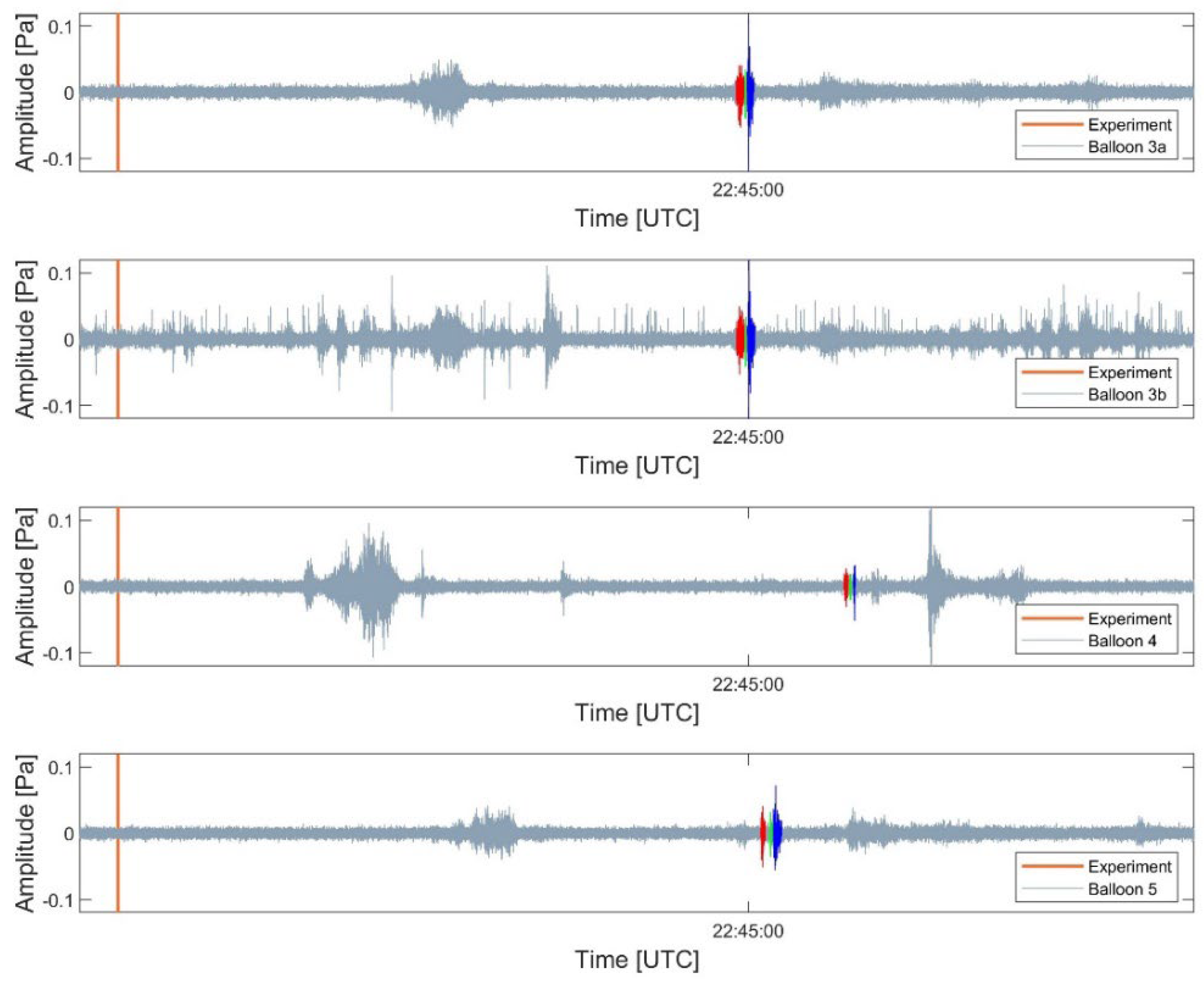
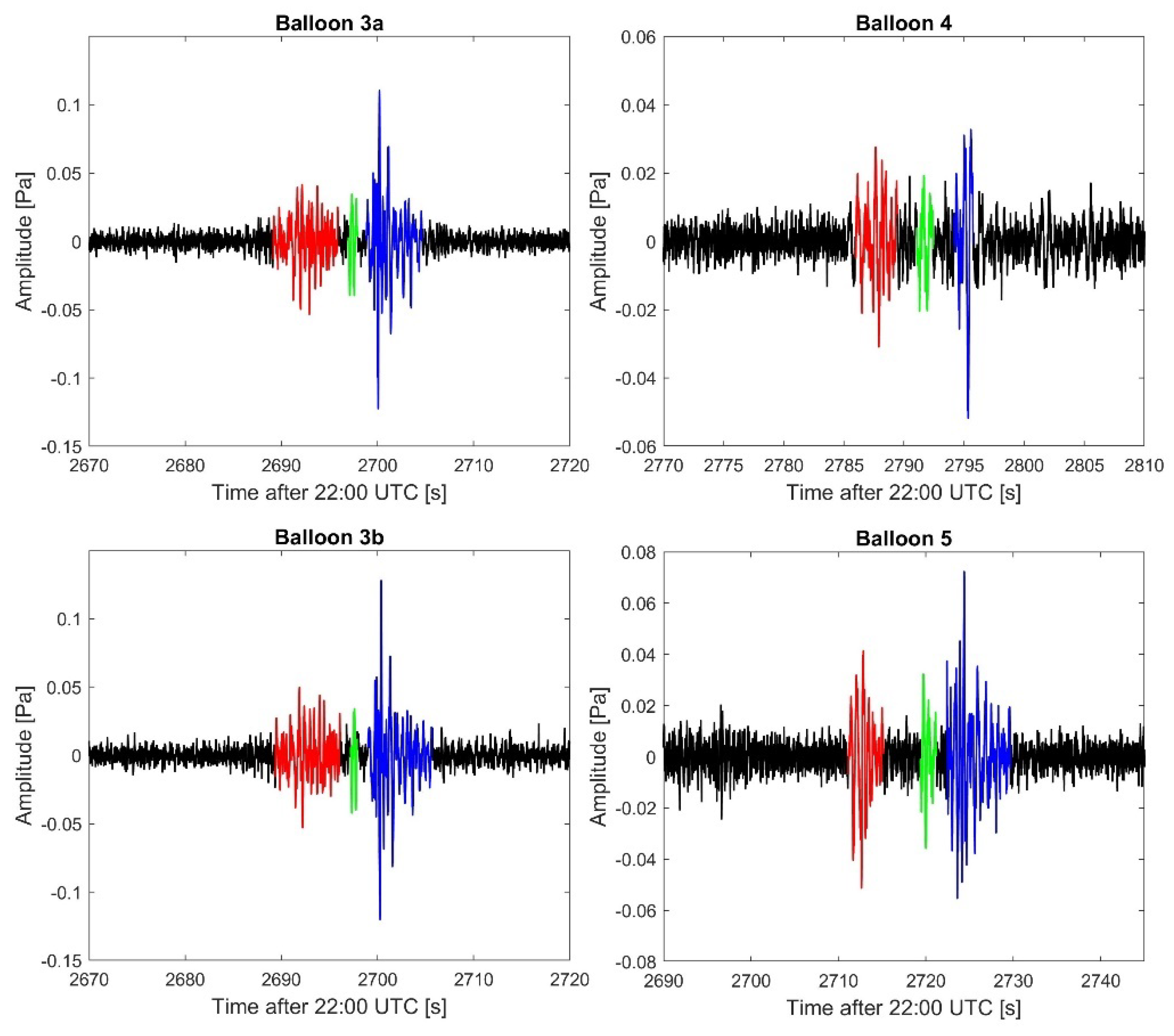
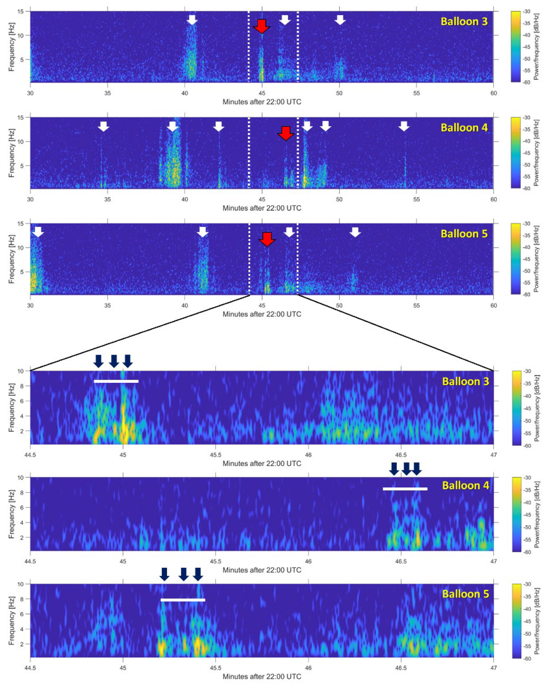
3.2. Infrasound Signal Detections

We examined the raw and filtered (high-pass Butterworth) timeseries to look for the signals generated by Apollo within the detection probability time window established following the approach described in the previous section. Earlier studies [12,15,16] reported a relatively quiet background and fairly low noise levels in the lower stratosphere, which is conducive to detecting far-field and low signal-to-noise (SNR) signals by floating sensing platforms. As balloons are carried by wind, there should be virtually zero wind noise [12,14].
As mentioned in Section 2.2, vertical oscillations of the balloons create long period waves [15]. However, these data were much noisier than expected at all three solar hot air balloons, indicating that most of the noise was not self-generated (e.g., due to issues related to instruments or the flight system). The origin of this additional noise beyond the contribution of self-generated noise remains unresolved. Depending on signal-to-noise ratio (SNR), noisy data may interfere with qualitative, visual signal identification generally employed as the first order step to search for possible detections. However, the presence of noise in our study was not substantial enough to adversely affect the signal detection. A further detailed investigation into that topic is needed and therefore, we will not further discuss it here.
The infrasonic signature from Apollo was sufficiently unambiguous and consistent across the sensors, which aided in its identification and time picks. The signals were found on all four sensors–two sensors were arranged into a 2-element vertical array on Balloon 3. Figure 5 shows the filtered time series (high-pass filter cut-off frequency was 1 Hz). The vertical orange line corresponds to the detonation time (22:35 UTC). The top two panels show the time series from Balloon 3–the original payload (a) and the additional payload suspended beneath the first (b). The bottom two panels are the time series for Balloons 4 and 5. It can be readily seen from the figure that the signal was first detected at Balloon 3, followed by Balloon 5, and then Balloon 4.
The signals received by all sensors show three distinct phases: two readily discernable phases (plotted in red and blue for better visualization), and a third, significantly weaker phase (plotted in green) in-between those. Considering that standard array processing methods were not applicable to our data and the Apollo-generated signature was readily discernable, a rigorous approach to establish time picks was not necessitated. It would be straight forward to manually select time picks at a same feature at all four sensors. To mitigate any subjectivity bias, we employed a simple approach to select time picks in a consistent and easy to replicate manner across all waveforms. We measured the root-mean-square value of the amplitude (Arms) of the noise before and after the signal, within a 10–20 s long ‘quiet’ time segment or where the ambient pressure levels appeared overall featureless (i.e., no significant spikes). The onset and duration of each phase were hand-picked where the signal amplitude was greater than some predetermined amplitude cutoff for at least two consecutive full cycles. Upon initial testing, this amplitude cutoff was set at 4 Arms; it served to exclude noise and include apparent signal in the filtered timeseries. This choice of the lower end amplitude threshold yielded robust and self-consistent time picks across all timeseries. The uncertainty in signal time picks is ±0.04 s, accounting for user inputs and sampling rate limitations.
We consider the most prominent phase (blue), which arrived last, to be the dominant or main phase, since it has the largest Hilbert envelope [35]. The time difference between the onset of the first and third (last) phase is between 8 s and 11 s, depending on the sensor. The speeds of the solar hot air balloons at the time of airwave detection were 30 (B3), 52 (B4), and 35 (B5) m/s. The signal parameters (arrival time, travel time, celerity, and signal duration) for each phase are listed in Table 1. We also included the location of the balloon at the onset of each phase, and the horizontal distance between the source and the balloons.
To estimate whether the signals from Apollo are direct or refracted arrivals, we took advantage of the vertical payload configuration suspended from Balloon 3. The signal arrival was detected by the top sensor first, at 22:44:49.14 UTC, followed by the sensor beneath it, at 22:44:49.37 UTC. That is a clear indication that this was a refracted wave coming from above rather than a direct wave coming from below. It should be noted that direct arrivals are not likely to occur at these distances.
Each signal was examined in more detail, and the dominant phase parameters measured (Table 2); these include the maximum signal amplitude (Amax) and peak-to-peak amplitude (AP2P) within the Hilbert envelope [35] and the dominant signal period (p) measured at maximum amplitude and zero crossings [36].
Figure 6 shows the zoomed-in timeseries region for a closer inspection of the signals. The detections by both sensors attached to Balloon 3 are shown as well (3a is the top sensor, and 3b is the bottom sensor). The time offset required to align these two waveforms is 0.2 s. The time axes are in seconds (after 22:00 UTC). The colored segments serve to delineate the individual arrival phases for visual purposes. Note that in this figure, the signals are not aligned, nor do they have the same time and amplitude scale. Following the same color scheme shown in Figure 5, the dominant phase is plotted in blue.
Figure 7 (top panel) shows a spectrogram for the three balloons during a 30-min time segment between 22:30 UTC and 23:00 UTC. The Nyquist frequency is 50 Hz, but we limit the view to 15 Hz for better visualization (the signals are shown with the red arrows). The bottom panel (Figure 7) shows the zoomed-in region with the 2.5-min-long time segment from 22:44:30 UTC until 23:47:00 UTC and up to 10 Hz, to better visualize the signals. The three phases are broadly shown with dark blue arrows. These are readily observable in the Balloons 3 and 5 spectrograms. There was an apparent loss of energy by the time the signal reached Balloon 4, and the second arrival is very weak. The signal recorded at Balloon 3 had the highest acoustic energy, and the signal from Balloon 4 exhibited the lowest frequency content and the lowest energy. Overall, the most acoustic energy from Apollo was concentrated below 5 Hz (Figure 7).
Other spikes of acoustic energy in the spectrogram, concentrated at low frequencies or more broadband, are shown with the white arrows. The examples of the former are the following time segments: 46–50 min (Balloon 3), 48–49 min (Balloon 4), and 47–48 min and 51 min (Balloon 5). The examples of the broadband energy content are also seen in all three balloons, in the following time segments: 40–41 min (Balloon 3), 38–40 min and 48 min (Balloon 4), and 30–31 min and 41–42 min (Balloon 5). The ‘broadband’ signals that appear somewhat similar (upon visual inspection) across all balloons are the three spikes seen close to the 40 min mark. The first arrival was at Balloon 4 (48–49 min), followed by Balloon 3 (40–41 min), and then Balloon 5 (41–42 min). Notably, the highest acoustic energy content and the longest duration were recorded at Balloon 4, and the weakest and shortest at Balloon 5, indicative of a source originating closest to Balloon 4, and seemingly in the opposite direction of Apollo. Moreover, the spike seen at 30–31 min (Balloon 5) also bears features, at least visually, similar to those at Balloon 4.
All these spikes in acoustic energy can be ruled out as signals from Apollo because of one or more of the following reasons: (1) the signals do not seem to be correlated across the balloon network (e.g., spikes do not appear on all balloons or have much different features across the balloon network); (2) the ‘signal’ timing does not correspond to that associated with Apollo (i.e., too early or too late), and (3) the arrivals indicate a general direction of the source being much different than that of Apollo (e.g., if there is an apparent arrival detected by Balloon 4 first, it cannot possibly originate from Apollo). However, it cannot be said with any certainty whether all or some of these spikes could be correlated and what their origin might be. Some of these spikes might be sporadic noise or resulting from an unknown source. A rigorous analysis, which is beyond the scope of this study, would be needed to illuminate possible sources.

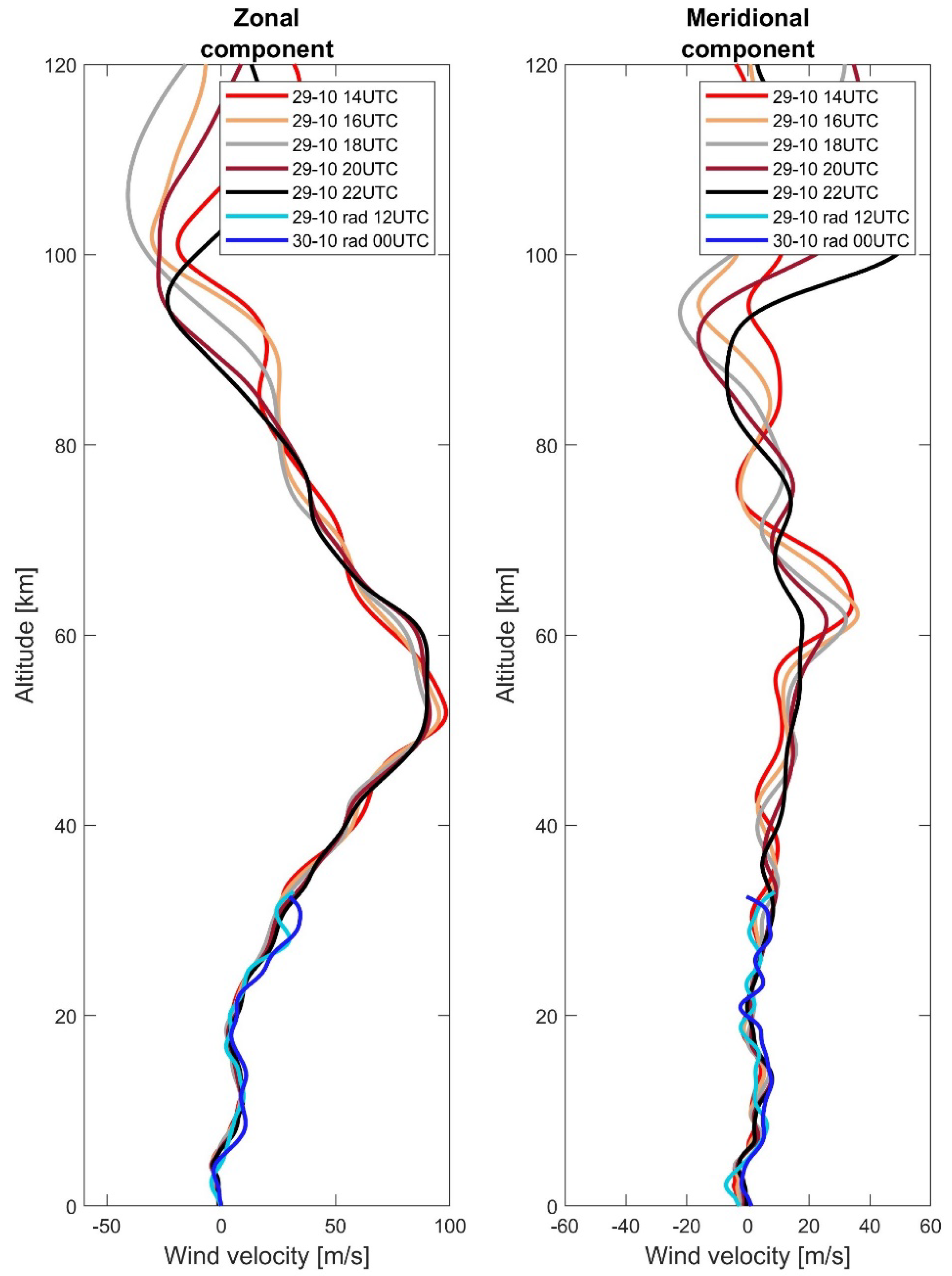
4. Propagation Modeling

We employed raytracing to verify our detection, as well as identify when and where along the balloon’s trajectory the signals are most likely to arrive. Raytracing was also utilized to investigate whether propagation paths (direct and/or refracted) to all or some portions of the flight trajectory exist, while taking into consideration temporal changes in the balloon’s location. Propagation modeling was carried out using the open source InfraGA/GeoAc raytracing package to search for “eigenrays” (rays connecting source and receiver) (see [37] for more details).
Wind fields can significantly affect airwave propagation [31]. For direct airwave arrivals, the atmospheric region extending from the surface up to the solar hot air balloon cruising altitude of ~20 km is of the most relevance. On the other hand, refracted airwaves are expected to turn over at altitudes between approximately 30 and 50 km. Thus, to accurately calculate airwave propagation and estimate arrivals, it is important to use the temperature and wind profiles that are representative of realistic atmospheric conditions for a given location, day, and time. At this time of the year, the stratospheric winds are predominantly eastward, and thus preferential infrasound ducting is also eastward [38]. We extracted atmospheric profiles generated by the Ground-to-Space (G2S) model [30] and provided by the National Center for Physical Acoustics. The geographic location selected for the G2S profile was the launch location of the balloons, and the time was the hour of the Apollo detonation (22:00 UTC). To examine the variation of the atmospheric model over several hours on that day, we collected a sequence of climatological (G2S) profiles, 1 h apart, from 13:00 UTC to 23:00 UTC. In Figure 8, we show a representative sample of the zonal (east–west) and meridional (north–south) components of the wind field from 14:00 to 22:00 UTC in 2-h increments. We also extracted the radiosonde data from the nearby station situated in Las Vegas (station code: USM00072388; 36.05° N, −115.18° E). These data are customarily collected every 12 h, at 00:00 UTC and 12:00 UTC daily, and extend to approximately 30 km altitude. We plotted the radiosonde profiles alongside the G2S model. Here, the radiosonde data closely follow that of the model atmosphere. This is not always the case–typically, the greatest discrepancies between the model and real data are in the lower regions of the atmosphere (<~20 km). It is possible to spline the radiosonde data to the model atmosphere, but we opted against that for two reasons: (1) at greater altitudes, radiosonde data might be subject to higher uncertainties in the measurement, and (2) we have established that the radiosonde data follow the model atmosphere very well, supporting the notion that the G2S model is suitable for raytracing as is. Therefore, we used the climatological data (G2S) for propagation modeling.
It should be noted that the balloon float speeds were from ~30 m/s (B3 and B5) up to ~50 m/s (B4). The float speed of Balloon 4 was substantially greater than any of the atmospheric profiles (climatological or instrumental) we collected for 29 October 2020. Since the data logger provided the balloon speed and direction, we used that information to derive the zonal and meridional components of the horizonal drift velocity for each balloon. In Figure 9 we compared the G2S model atmosphere (black line) and the horizonal drift components for each balloon from the moment they were launched and up to 23:59 UTC on 29 October 2020. Considering that the G2S profiles from 14:00 UTC to 22:00 UTC are very similar (to within ~10 m/s), from the ground up to ~50 km, we plotted one G2S profile (22:00 UTC). The balloon drift velocity data points are colored according to the UTC hour during which they were collected. The balloon data show that westerly winds at the balloon float altitudes were much stronger than that predicted by the G2S model or even measured by radiosonde. Additionally, there are numerous fluctuations in the horizontal motion velocities during the balloon ascent; these were not present in either the radiosonde or G2S profiles. Some of these fluctuations are reminiscent of gravity wave perturbations to the wind field [12,15,39].
Raytracing results suggest that there exist predicted ray propagation paths for all three balloons along the entire portion of the trajectory that falls within the detection probability time window. The arrivals were estimated to first occur at Balloon 3, followed by Balloon 5 and then Balloon 4, consistent with the observations. Moreover, all modelled eigenrays are refracted rays, in line with that observed. Raytracing predicts one and in some cases at most two rays for all sampled points along the balloon trajectory. In the case of multiple rays, travel times are nearly identical, and none of them are consistent with well-defined phases that are separated by several seconds. Thus, while raytracing does readily predict eigenrays related to the trajectory portion of interest, it cannot account for multiple signal phases as observed. In Figure 10, we plotted the eigenrays corresponding to the timing of the first observed airwave arrival detected by the three floating sensors. Turning heights for these eigenrays are 48.9 km (B3), 49.9 km (B4), and 49.3 km (B5).

5. Discussion

In general, infrasound signal amplitude decreases with range, also readily seen in our data (Figure 6). The peak-to-peak signal amplitude is the largest at Balloon 3 (0.233 Pa), and the smallest at Balloon 4 (0.084 Pa). In a weakly nonlinear propagation, the wave period is expected to increase as a function of range due to dispersion that acts to ‘stretch’ it [40,41,42]. Here, we also observe longer airwave periods with increasing distance from the source. More detailed future studies are needed to examine wave propagation as it relates to elevated floating detectors and delineate if and where weakly nonlinear propagation might dominate over a linear regime and vice versa.
Overall, the most acoustic energy from Apollo is concentrated below 5 Hz (Figure 7), with the signal from Balloon 4 having the lowest frequency content. This is expected since Balloon 4 was 210 km away from the source at the time of detection, and Balloon 3 was the closest (173 km). Previous studies indicated that infrasound data collected by balloon-borne sensors should be less noisy than that collected at the ground. This is mainly because the free-floating sensors are carried by the wind and hence do not suffer from typical wind-induced noise as their ground-based counterparts [16,43]. However, this dataset appears to be quite noisy. Numerous ‘spikes’ exhibiting notable acoustic energy either at low or broadband frequencies are of unknown origin. Some of these might be sporadic noise or resulting from sources that are yet to be identified (e.g., industrial, aircraft, lightning, storms, bolides, etc.). Future dedicated studies are needed to establish their origin and better constrain sources of acoustic noise in the stratospheric region.
The signal with the largest celerity was that arriving to Balloon 4 (~323 m/s, compared to 312–315 m/s at the other two balloons), at the upper threshold of the conventional range for stratospheric arrivals [32,33]. Balloon 4 floated at a lower altitude than the other balloons, and where the zonal wind component was stronger than that at slightly higher altitudes (Figure 8). This balloon, despite being launched around the same time as the other two, was likely trapped in a vertically narrow, fast wind duct as it ascended. It also ended up on a different trajectory, diverging from Balloons 3 and 5. The cruising speed of Balloon 4 was 52 m/s, significantly faster than Balloons 3 and 5 (30 and 35 m/s, respectively). This suggests that the signal from Apollo was also likely channeled due to strong winds, explaining the high apparent celerity. This is consistent with numerous earlier studies, albeit for events at longer distances, which have shown that stratospheric winds play a primary role in modulating the transmission efficiency in this waveguide [44,45,46,47]. Faster (or slower) than conventional stratospheric arrivals have been documented before [3,46]. For example, Green et al. [3] examined infrasonic signals from munitions dump explosions for ground-to-ground source-receiver configurations and attributed the uncharacteristic travel times to gravity wave-induced small-scale perturbations. It should be noted that neither the radiosonde derived atmospheric profile nor the G2S model atmosphere profile capture the presence of the fast wind duct (likely jet stream). An earlier study [12] also found strong westerly winds which were not predicted by the G2S model.
Distinct arrival phases are often seen in far-field infrasound propagation mainly due to multipathing through different waveguides (e.g., stratospheric, thermospheric) [48,49,50]. For an airwave arriving to an elevated sensing platform at regional scales (<250 km), this is a less likely scenario. The fact that high-altitude drifting sensors are in a continuous state of motion gives rise to the question whether it is reasonable to entertain the hypothesis that these sensors might be ‘sampling’ different portions of the shock-generated airwave as they are floating along their path. However, a simple calculation that takes into account the observed arrival times for each phase, the balloon’s GPS location as a function of time, and the raytracing results removes any possibility of such a scenario. The balloons would have to travel at speeds that are at least an order of magnitude greater than their actual speed for the recorded signals to reflect this supposition. Instead, we hypothesize that small scale structures in the atmosphere (e.g., turbulence and gravity waves) [3,51,52,53] are responsible for the observed pattern in the signals recorded by the high-altitude floating receivers.
Multiple phases in infrasound signals at regional distances have been documented before for ground-to-ground sensing (both source and receiver are at the surface level) [3,54,55] and for a source-receiver configuration where one of these is elevated [34]. For example, previous studies (i.e., [3]) observed multipathing for signals undergoing multiple hops (distances > 950 km) and explained such behavior with small-scale perturbations caused by internal gravity waves (also see [56]). Hedlin and Walker [49] noted that small-scale internal gravity wave structures can lead to multipathing, as well as pulse lengthening. Both are observed in our data.
In terms of elevated sources, Silber and Brown [34] analyzed infrasound signals generated by meteoroids (altitudes from ~100 km down to ~40 km) at regional distances (<250 km). Meteoroids are high-altitude hypersonic sources and follow flight trajectories that extend 10 s of kilometers. For an elevated moving source and a stationary ground-based detector, two scenarios have been determined to lead to multiple arrivals: (1) ground stations ‘sampling’ two or more portions of the meteor trail, i.e., signals coming from different parts of the trajectory, and (2) infrasound wave generated at a single point but experiencing the effect of small-scale structures (e.g., gravity waves) in the atmosphere that result in multipathing [34]. In this study, the source-receiver configuration is reversed–the source is ground-based, while the receiver floats in the lower stratosphere. Therefore, only the second scenario is plausible.
Propagation modeling provides up to two possible eigenrays connecting the source and the receiver for every point along the flight trajectory that was examined (see Section 3.1). At these distances from the source, it is not expected that any arrivals would be direct. Indeed, all eigenrays are refracted from the lower stratosphere (~50 km altitude) towards the surface, approaching the floating sensors from above. These results indicate that none of the signal phases are thermospheric arrivals, thus reinforcing the notion that the observed phases are caused by small-scale structures in the atmosphere rather than propagation through the major waveguides. Silber and Brown [34] also demonstrated that small-scale perturbations play a significant role in signal prediction and detection from high altitude sources even at regional distances. A further investigation into this topic as it relates to high-altitude balloon infrasound is recommended for future detailed studies.
As mentioned in Section 3.1, the nature of the airborne sensor system is such that it presents immense challenges for traditional array processing. The temporal changes in sensor location, as well as immense vertical and horizontal separations between individual sensors impede traditional array processing efforts. Array processing techniques break down due to the significant time delays and degrading signal coherency associated with such large array apertures. Therefore, future studies should explore novel approaches that use time-dependent array configurations.

6. Conclusions

Three solar hot air balloons equipped with the infrasound sensor payload were successfully launched on 29 October 2020 with the aim to capture infrasonic signals generated by the Large Surface Explosion Coupling Experiment carried out at the Nevada National Security Site. The signals were recorded by all sensors, proving the effectiveness of a free flying sensing system to detect impulsive events at stratospheric altitudes. One solar hot air balloon was equipped with a double payload, where one sensor was suspended beneath another. This configuration helped in ascertaining that the airwave was a reflected arrival approaching from above rather than a direct arrival coming from below. Raytracing using a realistic atmosphere corroborated these observations, including signal travel times. At the time of the detection, the balloons were 173–210 km eastward from the source. The signals arrived in three phases indicative of multipathing, which we attribute to small scale perturbations in the atmosphere. This is further supported by the horizontal drift speeds of the balloons that show small scale fluctuations consistent with gravity wave perturbations to the wind field. Additionally, our dataset indicates that infrasonic noise in the stratospheric region is more complex than previously thought. Future studies should aim to characterize sources of noise, investigate the effect of small-scale perturbations on signal propagation, and explore novel approaches in array processing that would account for an array with continuously changing aperture and sensor elevations.

Author Contributions

Conceptualization, D.C.B.; methodology and formal analysis, E.A.S.; investigation, E.A.S. and M.R.G.; writing—original draft preparation and revision, E.A.S.; writing—review and editing, E.A.S., D.C.B. and M.R.G.; visualization, E.A.S.; project administration, D.C.B.; funding acquisition, D.C.B. All authors have read and agreed to the published version of the manuscript.

Funding

The experiment and follow-on research were supported by the Nuclear Arms Control Technology (NACT) program at the Defense Threat Reduction Agency (DTRA).

Data Availability Statement

Data collected as part of LSECE are under a two-year embargo and is anticipated to be available to the public at the IRIS Data Center (www.iris.edu) starting in 2023.

Acknowledgments

The Large Surface Explosion Coupling Experiment (LSECE) would not have been possible without the support of many people from several organizations. The authors wish to express our gratitude to the LSECE working group and multi-institutional and interdisciplinary group of scientists and engineers for the field experiment. Sandia National Laboratories is a multimission laboratory managed and operated by National Technology & Engineering Solutions of Sandia, LLC, a wholly owned subsidiary of Honeywell International Inc., for the U.S. Department of Energy’s National Nuclear Security Administration under contract DE-NA0003525. This paper describes objective technical results and analysis. Any subjective views or opinions that might be expressed in the paper do not necessarily represent the views of the U.S. Department of Energy or the United States Government. The authors thank the two anonymous reviewers and the editorial team for providing useful comments that helped improve this paper.

Conflicts of Interest

The authors declare no conflict of interest.

References

  1. Bedard, A.; Georges, T. Atmospheric infrasound. Acoust. Aust. 2000, 28, 47–52. [Google Scholar] [CrossRef]
  2. Silber, E.A.; ReVelle, D.O.; Brown, P.G.; Edwards, W.N. An estimate of the terrestrial influx of large meteoroids from infrasonic measurements. J. Geophys. Res. 2009, 114, E08006. [Google Scholar] [CrossRef] [Green Version]
  3. Green, D.N.; Vergoz, J.; Gibson, R.; Le Pichon, A.; Ceranna, L. Infrasound radiated by the Gerdec and Chelopechene explosions: Propagation along unexpected paths. Geophys. J. Int. 2011, 185, 890–910. [Google Scholar] [CrossRef] [Green Version]
  4. Matoza, R.S.; Hedlin, M.A.H.; Garcés, M.A. An infrasound array study of Mount St. Helens. J. Volcanol. Geotherm. Res. 2007, 160, 249–262. [Google Scholar] [CrossRef]
  5. Evans, L.B.; Bass, H.E.; Sutherland, L.C. Atmospheric Absorption of Sound: Theoretical Predictions. J. Acoust. Soc. Am. 1972, 51, 1565–1575. [Google Scholar] [CrossRef]
  6. Christie, D.R.; Campus, P. The IMS infrasound network: Design and establishment of infrasound stations. In Infrasound Monitoring for Atmospheric Studies; Springer: Berlin/Heidelberg, Germany, 2010; pp. 29–75. [Google Scholar]
  7. Evers, L.G.; Haak, H.W. The Characteristics of Infrasound, its Propagation and Some Early History. In Infrasound Monitoring for Atmospheric Studies; Le Pichon, A., Blanc, E., Hauchecorne, A., Eds.; Springer: Dordrecht, The Netherlands, 2010; pp. 3–27. [Google Scholar]
  8. Brachet, N.; Brown, D.; Le Bras, R.; Cansi, Y.; Mialle, P.; Coyne, J. Monitoring the earth’s atmosphere with the global IMS infrasound network. In Infrasound Monitoring for Atmospheric Studies; Springer: Berlin/Heidelberg, Germany, 2010; pp. 77–118. [Google Scholar]
  9. Wescott, J.W. Acoustic Detection of High-Altitude Turbulence; Michigan Univ. Ann Arbor: Ann Arbor, MI, USA, 1964; p. 62. [Google Scholar]
  10. Weaver, R.L.; McAndrew, J. The Roswell Report: Fact versus Fiction in the New Mexico Desert; 1428994920; Diane Publishing: Collingdale, PA, USA, 1995; p. 881. [Google Scholar]
  11. Bowman, D.C.; Young, E.F.; Krishnamoorthy, S.; Lees, J.M.; Albert, S.A.; Komjathy, A.; Cutts, J. Geophysical and Planetary Acoustics via Balloon Borne Platforms; Sandia National Lab. (SNL-NM): Albuquerque, NM, USA, 2018. [Google Scholar]
  12. Young, E.F.; Bowman, D.C.; Lees, J.M.; Klein, V.; Arrowsmith, S.J.; Ballard, C. Explosion-generated infrasound recorded on ground and airborne microbarometers at regional distances. Seismol. Res. Lett. 2018, 89, 1497–1506. [Google Scholar] [CrossRef]
  13. Poler, G.; Garcia, R.F.; Bowman, D.C.; Martire, L. Infrasound and gravity waves over the Andes observed by a pressure sensor on board a stratospheric balloon. J. Geophys. Res. Atmos. 2020, 125, e2019JD031565. [Google Scholar] [CrossRef]
  14. Bowman, D.C.; Lees, J.M. Upper Atmosphere Heating from Ocean-Generated Acoustic Wave Energy. Geophys. Res. Lett. 2018, 45, 5144–5150. [Google Scholar] [CrossRef]
  15. Bowman, D.C.; Albert, S.A. Acoustic event location and background noise characterization on a free flying infrasound sensor network in the stratosphere. Geophys. J. Int. 2018, 213, 1524–1535. [Google Scholar] [CrossRef] [Green Version]
  16. Krishnamoorthy, S.; Bowman, D.C.; Komjathy, A.; Pauken, M.T.; Cutts, J.A. Origin and mitigation of wind noise on balloon-borne infrasound microbarometers. J. Acoust. Soc. Am. 2020, 148, 2361. [Google Scholar] [CrossRef]
  17. Brissaud, Q.; Krishnamoorthy, S.; Jackson, J.M.; Bowman, D.C.; Komjathy, A.; Cutts, J.A.; Zhan, Z.; Pauken, M.T.; Izraelevitz, J.S.; Walsh, G.J. The First Detection of an Earthquake from a Balloon Using Its Acoustic Signature. Geophys. Res. Lett. 2021, 48, e2021GL093013. [Google Scholar] [CrossRef] [PubMed]
  18. Garcia, R.F.; Klotz, A.; Hertzog, A.; Martin, R.; Gérier, S.; Kassarian, E.; Bordereau, J.; Venel, S.; Mimoun, D. Infrasound from Large Earthquakes Recorded on a Network of Balloons in the Stratosphere. Geophys. Res. Lett. 2022, 49, e2022GL098844. [Google Scholar] [CrossRef]
  19. Podglajen, A.; Le Pichon, A.; Garcia, R.F.; Gérier, S.; Millet, C.; Bedka, K.; Khlopenkov, K.; Khaykin, S.; Hertzog, A. Stratospheric Balloon Observations of Infrasound Waves From the 15 January 2022 Hunga Eruption, Tonga. Geophys. Res. Lett. 2022, 49, e2022GL100833. [Google Scholar] [CrossRef]
  20. Bowman, D.C. Airborne Infrasound Makes a Splash. Geophys. Res. Lett. 2021, 48, e2021GL096326. [Google Scholar] [CrossRef]
  21. Bowman, D.C.; Krishnamoorthy, S. Infrasound from a buried chemical explosion recorded on a balloon in the lower stratosphere. Geophys. Res. Lett. 2021, 48, e2021GL094861. [Google Scholar] [CrossRef]
  22. Bowman, D.C.; Norman, P.E.; Pauken, M.T.; Albert, S.A.; Dexheimer, D.; Yang, X.; Krishnamoorthy, S.; Komjathy, A.; Cutts, J.A. Multihour stratospheric flights with the heliotrope solar hot-air balloon. J. Atmos. Ocean. Technol. 2020, 37, 1051–1066. [Google Scholar] [CrossRef]
  23. Anderson, J.F.; Johnson, J.B.; Bowman, D.C.; Ronan, T.J. The Gem infrasound logger and custom-built instrumentation. Seismol. Res. Lett. 2018, 89, 153–164. [Google Scholar] [CrossRef]
  24. Bar-Yehuda, Z. Plot_Google_Map. 2022. Available online: https://github.com/zoharby/plot_google_map (accessed on 20 November 2022).
  25. Rost, S.; Thomas, C. Array seismology: Methods and applications. Rev. Geophys. 2002, 40, 2-1-2-27. [Google Scholar] [CrossRef] [Green Version]
  26. Evers, L.G.; Haak, H.W. Tracing a meteoric trajectory with infrasound. Geophys. Res. Lett. 2003, 30, 1–4. [Google Scholar] [CrossRef]
  27. Garces, M.A. On infrasound standards, Part 1 time, frequency, and energy scaling. InfraMatics 2013, 2, 23. [Google Scholar] [CrossRef]
  28. Beer, T. Atmospheric Waves; Halsted Press: New York, NY, USA; Adam Hilger, Ltd.: London, UK, 1974; Volume 1, p. 315. [Google Scholar]
  29. Negraru, P.T.; Herrin, E.T. On Infrasound Waveguides and Dispersion. Seismol. Res. Lett. 2009, 80, 565–571. [Google Scholar] [CrossRef]
  30. Drob, D.P.; Picone, J.M.; Garces, M. Global morphology of infrasound propagation. J. Geophys. Res. 2003, 108, 1–12. [Google Scholar] [CrossRef]
  31. Drob, D.P.; Garces, M.; Hedlin, M.; Brachet, N. The Temporal Morphology of Infrasound Propagation. Pure Appl. Geophys. 2010, 167, 437–453. [Google Scholar] [CrossRef]
  32. Negraru, P.T.; Golden, P.; Herrin, E.T. Infrasound Propagation in the “Zone of Silence”. Seismol. Res. Lett. 2010, 81, 614–624. [Google Scholar] [CrossRef]
  33. Kulichkov, S. On infrasonic arrivals in the zone of geometric shadow at long distances from surface explosions. In Proceedings of the Ninth Annual Symposium on Long-Range Propagation, Amsterdam, The Netherlands, 14–15 September 2000; pp. 238–251. [Google Scholar]
  34. Silber, E.A.; Brown, P.G. Optical observations of meteors generating infrasound—I: Acoustic signal identification and phenomenology. J. Atmos. Sol. Terr. Phys. 2014, 119, 116–128. [Google Scholar] [CrossRef] [Green Version]
  35. Dziewonski, A.; Hales, A. Numerical analysis of dispersed seismic waves. Seismol. Surf. Waves Earth Oscil. 1972, 11, 39–84. [Google Scholar]
  36. Revelle, D.O. Historical Detection of Atmospheric Impacts by Large Bolides Using Acoustic-Gravity Wavesa. Ann. N. Y. Acad. Sci. 1997, 822, 284–302. [Google Scholar] [CrossRef] [Green Version]
  37. Blom, P.; Waxler, R. Modeling and observations of an elevated, moving infrasonic source: Eigenray methods. J. Acoust. Soc. Am. 2017, 141, 2681–2692. [Google Scholar] [CrossRef]
  38. Le Pichon, A.; Vergoz, J.; Blanc, E.; Guilbert, J.; Ceranna, L.; Evers, L.; Brachet, N. Assessing the performance of the International Monitoring System’s infrasound network: Geographical coverage and temporal variabilities. J. Geophys. Res. 2009, 114, D08112. [Google Scholar] [CrossRef] [Green Version]
  39. Chunchuzov, I.; Kulichkov, S.; Perepelkin, V.; Popov, O.; Firstov, P.; Assink, J.D.; Marchetti, E. Study of the wind velocity-layered structure in the stratosphere, mesosphere, and lower thermosphere by using infrasound probing of the atmosphere. J. Geophys. Res. Atmos. 2015, 120, 8828–8840. [Google Scholar] [CrossRef]
  40. Green, D.N.; Nippress, A. Infrasound signal duration: The effects of propagation distance and waveguide structure. Geophys. J. Int. 2019, 216, 1974–1988. [Google Scholar] [CrossRef]
  41. Dumond, J.W.M.; Cohen, R.; Panofsky, W.K.H.; Deeds, E. A Determination of the Wave Forms and Laws of Propagation and Dissipation of Ballistic Shock Waves. J. Acoust. Soc. Am. 1946, 18, 97–118. [Google Scholar] [CrossRef] [Green Version]
  42. ReVelle, D. Acoustics of Meteors-effects of the atmospheric temperature and wind structure on the sounds produced by meteors. PhD Thesis, Michigan University Ann Arbor, Ann Harbor, MI, USA, 1974. [Google Scholar]
  43. Bowman, J.; Baker, G.; Bahavar, M. Infrasound Station Ambient Noise Estimates. In Proceedings of the 26th Seismic Research Review, Orlando, FL, USA, 21–23 September 2004. [Google Scholar]
  44. Reed, J.W. Climatology of Airblast Propagation from Nevada Test Site Nuclear Airblasts; Tech. Rep. SC-RR-69-572; SANDIA CORP: Albuquerque, NM, USA, 1969. [Google Scholar]
  45. Garces, M.A.; Hansen, R.A.; Lindquist, K.G. Traveltimes for infrasonic waves propagating in a stratified atmosphere. Geophys. J. Int. 1998, 135, 255–263. [Google Scholar] [CrossRef] [Green Version]
  46. Kulichkov, S. Long-range propagation and scattering of low-frequency sound pulses in the middle atmosphere. Meteorol. Atmos. Phys. 2004, 85, 47–60. [Google Scholar] [CrossRef]
  47. Kulichkov, S. On the Prospects for Acoustic Sounding of the Fine Structure of the Middle Atmosphere. In Infrasound Monitoring for Atmospheric Studies; Le Pichon, A., Blanc, E., Hauchecorne, A., Eds.; Springer: Dordrecht, The Netherlands, 2009; pp. 511–540. [Google Scholar]
  48. Silber, E.A.; Le Pichon, A.; Brown, P.G. Infrasonic detection of a near-Earth object impact over Indonesia on 8 October 2009. Geophys. Res. Lett. 2011, 38, L12201. [Google Scholar] [CrossRef]
  49. Hedlin, M.A.H.; Walker, K.T. A study of infrasonic anisotropy and multipathing in the atmosphere using seismic networks. Philos. Trans. R. Soc. A Math. Phys. Eng. Sci. 2013, 371, 20110542. [Google Scholar] [CrossRef] [Green Version]
  50. Kulichkov, S.; Chunchuzov, I.; Bush, G.; Perepelkin, V. Physical modeling of long-range infrasonic propagation in the atmosphere. Izv. Atmos. Ocean. Phys. 2008, 44, 175–186. [Google Scholar] [CrossRef]
  51. Gibson, R.G.; Drob, D.P.; Broutman, D.; Winslow, N.W. Advancement of techniques for modeling the effects of atmospheric gravity-wave-induced inhomogeneities on infrasound propagation. In Proceedings of the 2010 Monitoring Research Review: Ground-Based Nuclear Explosion Monitoring Technologies, Orlando, FL, USA, 21–23 September 2010. [Google Scholar]
  52. Norris, D.; Gibson, R.; Bongiovanni, K. Numerical Methods to Model Infrasonic Propagation Through Realistic Specifications of the Atmosphere. In Infrasound Monitoring for Atmospheric Studies; Le Pichon, A., Blanc, E., Hauchecorne, A., Eds.; Springer: Dordrecht, The Netherlands, 2010; pp. 541–573. [Google Scholar]
  53. Chunchuzov, I. Influence of internal gravity waves on sound propagation in the lower atmosphere. Meteorol. Atmos. Phys. 2004, 85, 61–76. [Google Scholar] [CrossRef]
  54. Pilger, C.; Streicher, F.; Ceranna, L.; Koch, K. Application of propagation modeling to verify and discriminate ground-truth infrasound signals at regional distances. InfraMatics 2013, 2013, 39–55. [Google Scholar] [CrossRef] [Green Version]
  55. Ceranna, L.; Le Pichon, A.; Green, D.N.; Mialle, P. The Buncefield explosion: A benchmark for infrasound analysis across Central Europe. Geophys. J. Int. 2009, 177, 491–508. [Google Scholar] [CrossRef] [Green Version]
  56. Kulichkov, S.N.; Chunchuzov, I.P.; Popov, O.I. Simulating the influence of an atmospheric fine inhomogeneous structure on long-range propagation of pulsed acoustic signals. Izv. Atmos. Ocean. Phys. 2010, 46, 60–68. [Google Scholar] [CrossRef]
Figure 1. Solar hot air balloon launch. The payload and parachute are shown with the arrows. The balloon envelope size is 6 m.
Remotesensing 15 00542 g001
Figure 2. Balloon flight tracks on 29 October. Balloons 3, 4, and 5 are denoted with the B3, B4, and B5 labels, respectively. Balloon 2 is not shown because it suffered a mechanical failure. The map was generated using Google Maps and a modified version of the MATLAB code written by Bar-Yehuda [24].
Remotesensing 15 00542 g002
Figure 3. Altitudes of solar hot air balloons as a function of time. The detonation time is denoted with the vertical line.
Remotesensing 15 00542 g003
Figure 4. Lateral separations between the balloon pairs as a function of time, from 18:00 UTC to 23:59 UTC. The time of detonation is denoted with the vertical line. We note that the plot includes only the natural buoyancy phase of the balloon flight (the ascent and descent phases have not been plotted).
Remotesensing 15 00542 g004
Figure 5. Filtered (high-pass Butterworth, >1 Hz) timeseries from all four sensors. The top two are from the 2-element vertical array suspended from Balloon 3. The top and bottom sensors are denoted as Balloon 3a and Balloon 3b, respectively. The signal exhibits multiple phases–the three phases are plotted in red, green and blue for better visualization. The vertical orange line denotes the detonation time (22:35 UTC). The amplitude scale is the same in all panels.
Remotesensing 15 00542 g005
Figure 6. Zoomed-in view of the signals. The colored segments are included for visual purposes to delineate the individual arrival phases. Note that the signals are not aligned, nor do they have the same amplitude and time scale.
Remotesensing 15 00542 g006
Figure 7. Spectrogram for the period between 22:30 UTC and 23:00 UTC (top panel), and up to 15 Hz. The red arrows point to the signals from Apollo. The white arrows indicate acoustic energy spikes associated with noise and/or signals of unknown origin. The zoomed-in region between 22:44:30 UTC and 23:47:00 UTC (bottom panel) and up to 10 Hz highlights the Apollo signals, which are denoted with the white bars and dark blue arrows.
Remotesensing 15 00542 g007
Figure 8. Example of G2S wind profiles plotted alongside radiosonde profiles for 29–30 October 2020. Radiosonde data extend to about 30 km altitude.
Remotesensing 15 00542 g008
Figure 9. The horizontal motion of the solar hot air balloons in the form of the zonal and meridional velocity components. The horizontal motion points are colored according to the data collection time (in UTC). For comparison, we also plotted the G2S model atmospheric profile at 22:00 UTC.
Remotesensing 15 00542 g009
Figure 10. Raytracing results. Plotted are the eigenrays consistent with the observed arrival times of the first phase at all three floating sensors. The source is shown by the red triangle.
Remotesensing 15 00542 g010
Table 1. List of the signal parameters associated with the three phases detected by each sensor. The first column lists the balloon numbers. 3a and 3b are the top and bottom sensors, respectively, attached to Balloon 3. Starting with the second column, the signal parameters are: arrival time, balloon locations at the onset of each arrival (latitude, longitude, altitude), source-receiver distance along great circle, signal celerity, and signal duration.
BalloonSignal Arrival Time Signal Travel TimeBalloon LatitudeBalloon LongitudeBalloon AltitudeDistanceSignal CeleritySignal Duration
[hh:mm:ss][s][°][°][km][km][m/s][s]
3a22:44:49.14554.836.95912−114.1296520.99173.1312.06.8
22:44:56.97562.736.95905−114.1290920.99173.1307.61.0
22:44:58.85564.636.95903−114.1289020.99173.1306.65.8
3b22:44:49.37555.136.95912−114.1296520.99173.1311.86.8
22:44:57.21562.936.95905−114.1290920.99173.1307.60.7
22:44:59.03564.736.95903−114.1289020.99173.2306.66.6
422:46:25.98651.737.58252−113.7608919.61210.6323.23.5
22:46:31.07656.837.58252−113.7609119.61210.6320.71.4
22:46:34.19659.937.58255−113.7611619.59210.6319.21.6
522:45:11.15576.936.84854−114.0532022.26181.6314.84.0
22:45:19.39585.136.84848−114.0523022.26181.7310.51.8
22:45:22.42588.136.84846−114.0519622.26181.7308.97.3
Table 2. Signal measurements associated with the dominant phase.
BalloonPeak Amplitude, AmaxP2P AmplitudePeriod at Amax
[Pa][Pa][s]
3a0.12180.23280.37 ± 0.06
3b0.12670.24620.37 ± 0.07
40.05170.08440.54 ± 0.04
50.07240.12100.48 ± 0.06
Disclaimer/Publisher’s Note: The statements, opinions and data contained in all publications are solely those of the individual author(s) and contributor(s) and not of MDPI and/or the editor(s). MDPI and/or the editor(s) disclaim responsibility for any injury to people or property resulting from any ideas, methods, instructions or products referred to in the content.

