
Infrasound and Low-Audible Acoustic Detections from a Long-Term Microphone Array Deployment in Oklahoma

Abstract
:1. Introduction
2. Materials and Methods
2.1. Infrasound Array
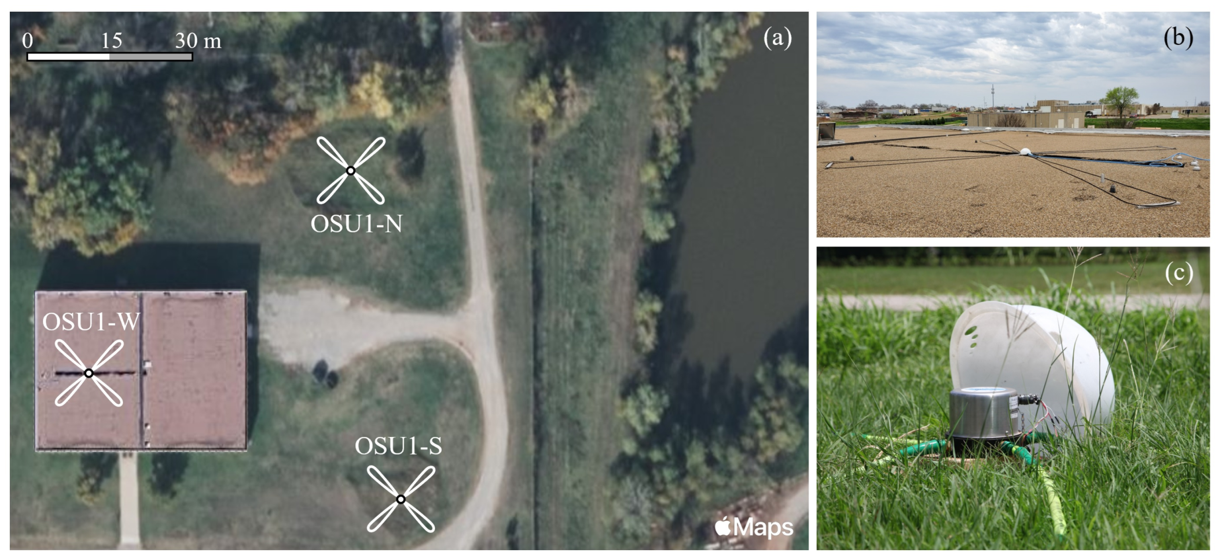
2.1.1. Layout and Sensors
2.1.2. Calibration
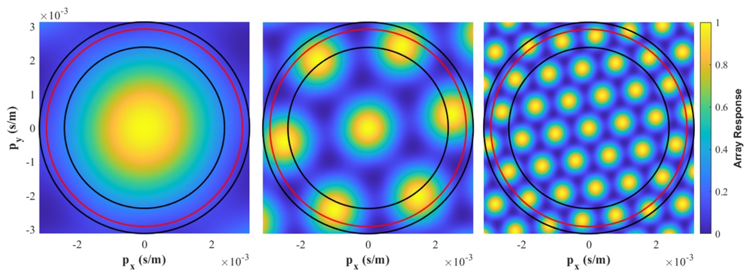
2.1.3. Array Response
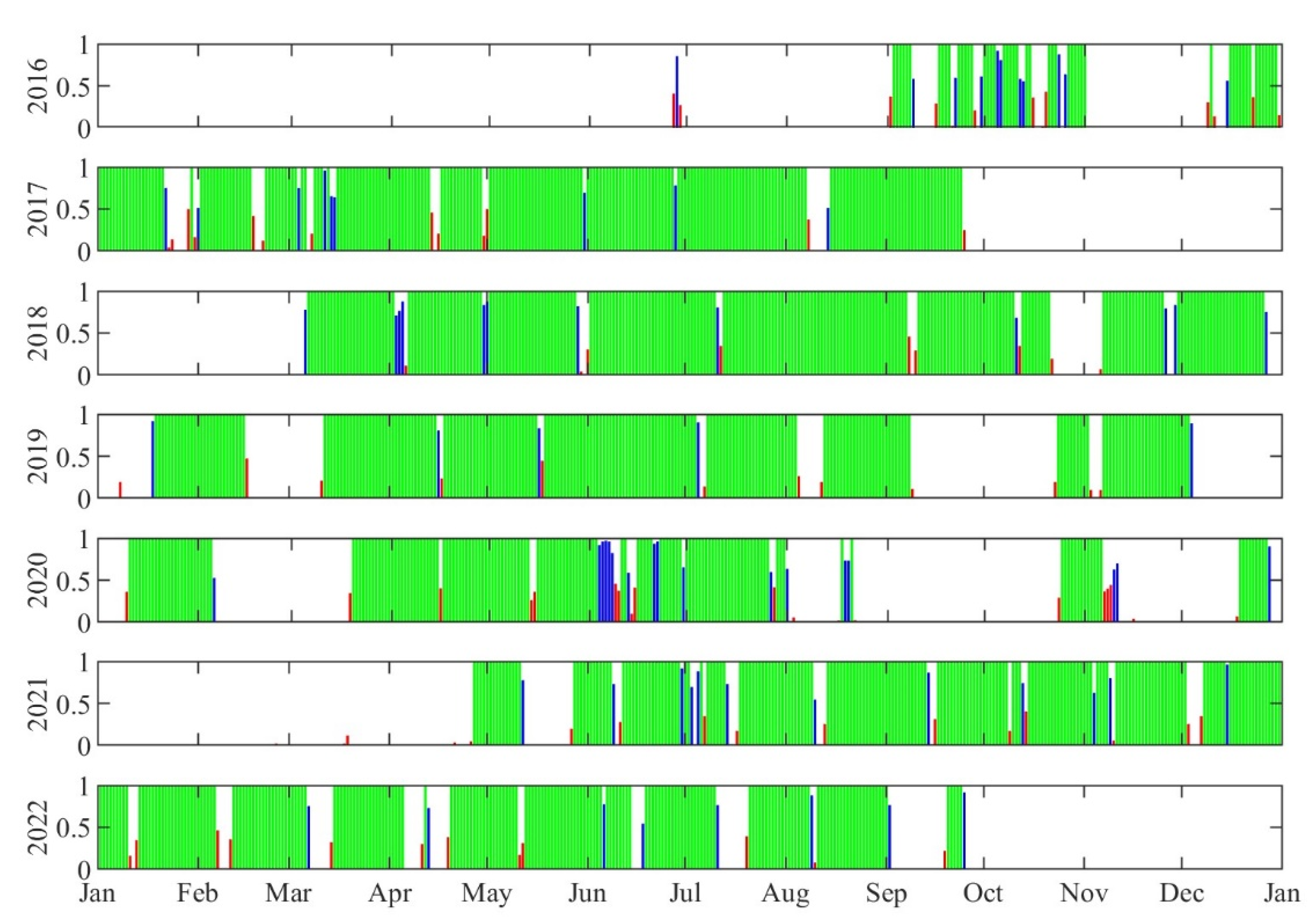
2.1.4. Operation
2.2. Ground Conditions
2.3. Signal Processing
3. Results
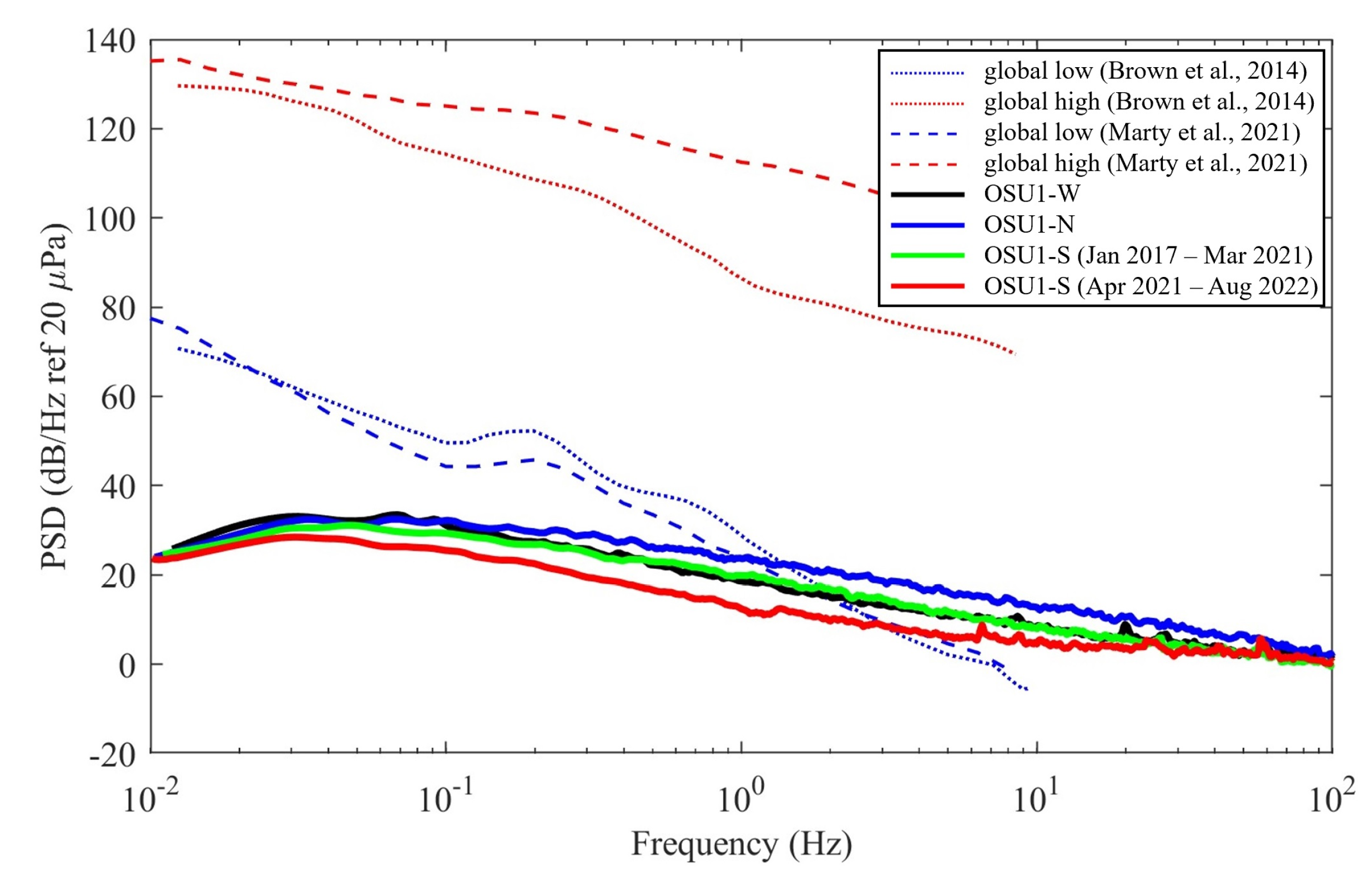
3.1. Ambient Noise
3.1.1. Noise Model
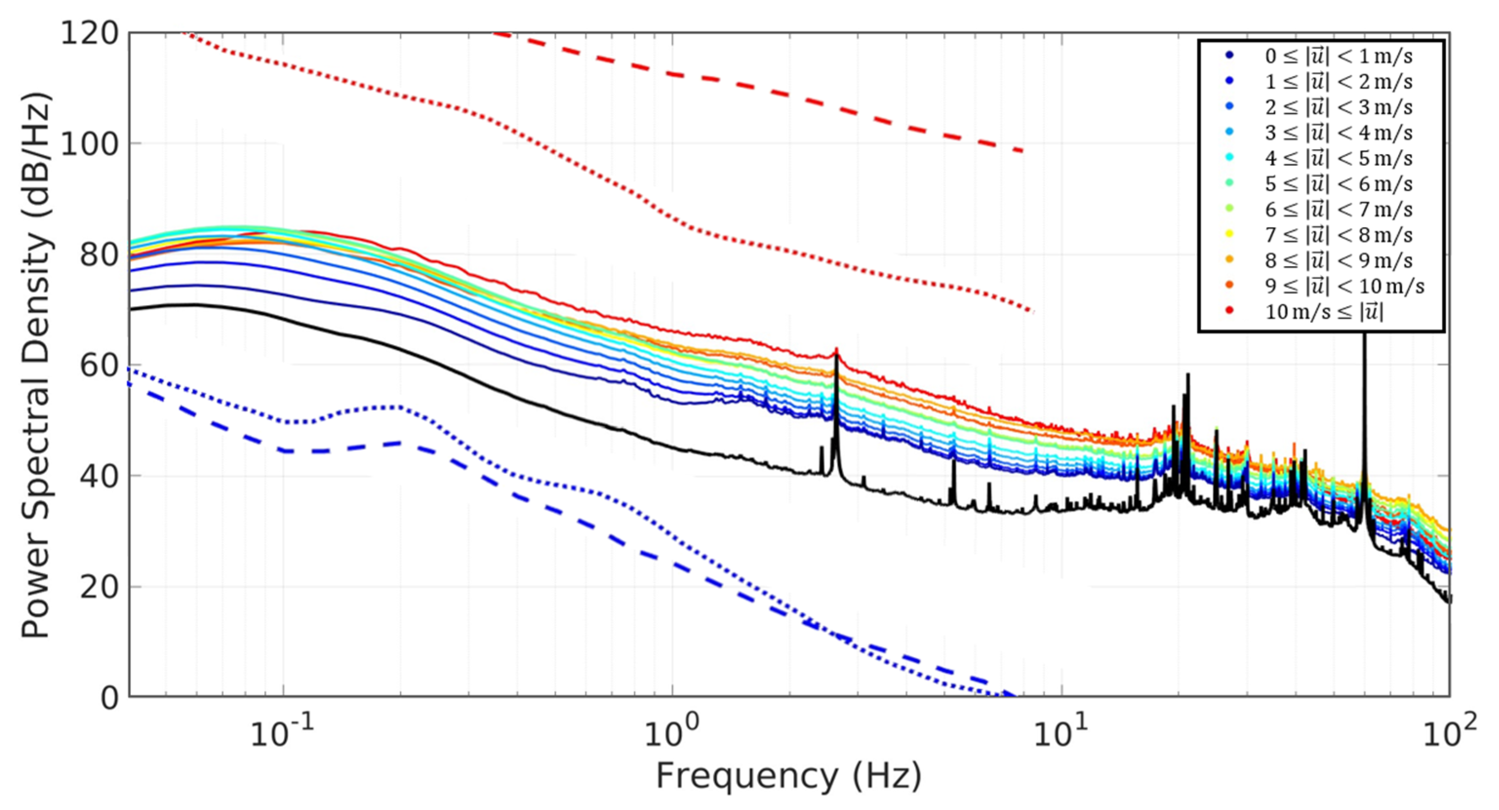
3.1.2. Wind Speed Dependence
3.1.3. Semi-Regular Local Noise Sources
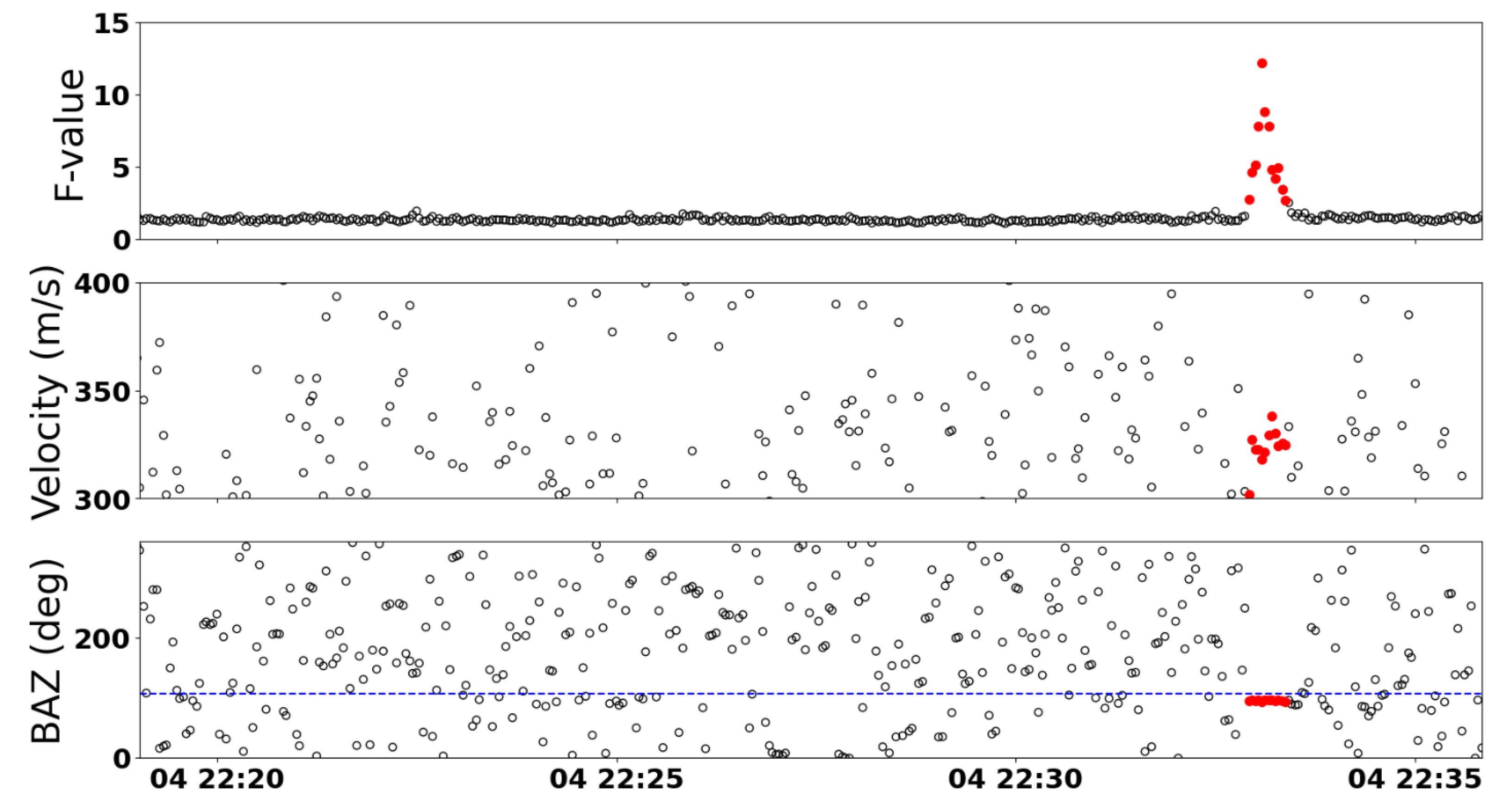
3.2. Examples of Event Detections
3.2.1. Microbaroms
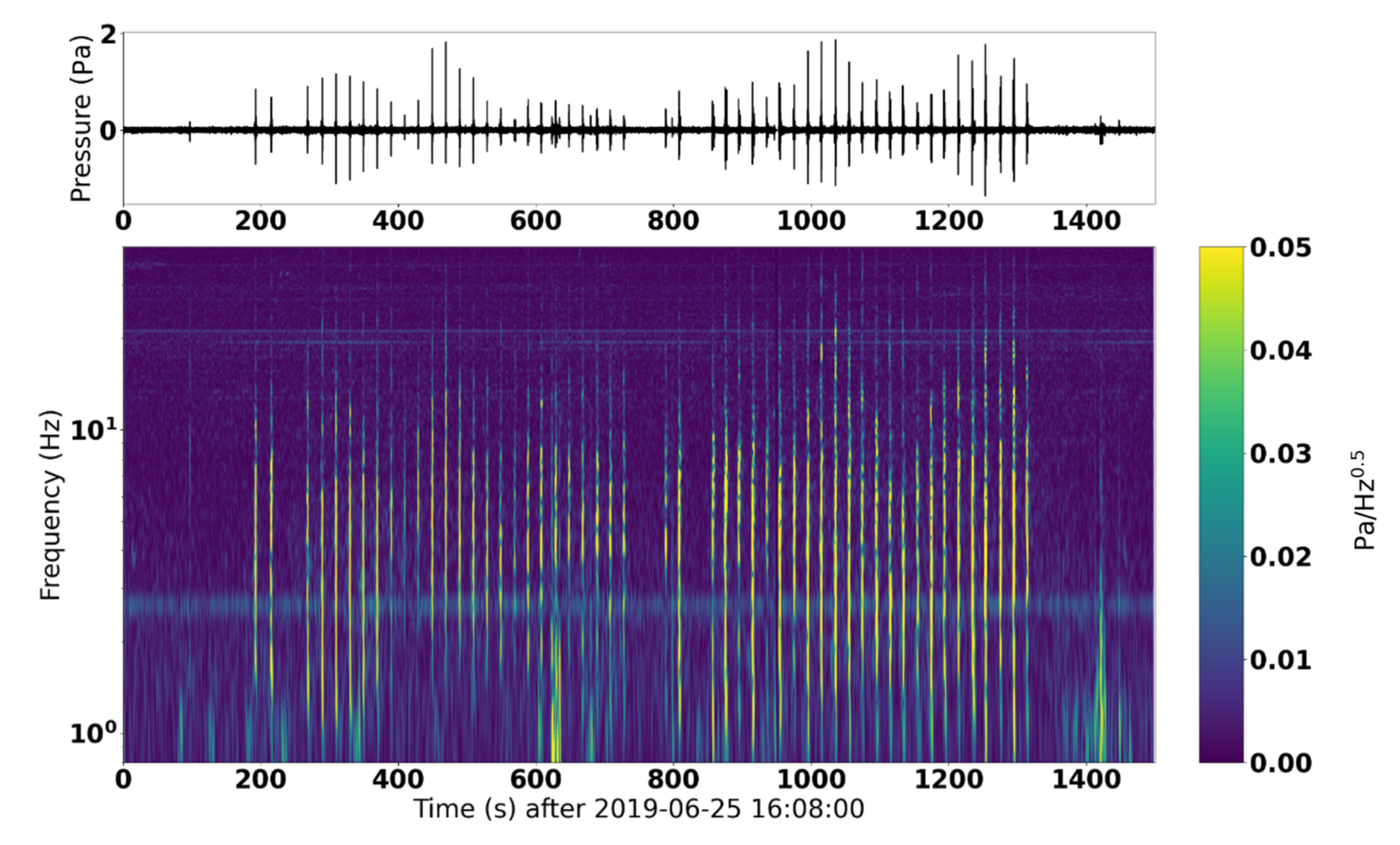
3.2.2. Fireworks
3.2.3. Aircraft
3.2.4. Explosions
3.2.5. Bolides
3.2.6. Earthquakes
3.2.7. Severe Weather
4. Discussion
5. Conclusions
Author Contributions
Funding
Data Availability Statement
Acknowledgments
Conflicts of Interest
References
- Brock, F.V.; Crawford, K.C.; Elliott, R.L.; Cuperus, G.W.; Stadler, S.J.; Johnson, H.L.; Eilts, M.D. The Oklahoma Mesonet: A technical overview. J. Atmos. Ocean Technol. 1995, 12, 5–19. [Google Scholar] [CrossRef]
- Zhang, H.; Jin, M.S.; Leach, M. A study of the Oklahoma City urban heat island effect using a WRF/single-layer urban canopy model, a joint urban 2003 field campaign, and MODIS satellite observations. Climate 2017, 5, 72. [Google Scholar] [CrossRef] [Green Version]
- Wulfmeyer, V.; Turner, D.D.; Baker, B.; Banta, R.; Behrendt, A.; Bonin, T.; Brewer, W.A.; Buban, M.; Choukulkar, A.; Dumas, E.; et al. A new research approach for observing and characterizing land-atmosphere feedback. Bull. Am. Meteorol. Soc. 2018, 99, 1639–1667. [Google Scholar] [CrossRef]
- Asher, E.; Thornberry, T.; Fahey, D.W.; McComiskey, A.; Carslaw, K.; Grunau, S.; Chang, K.-L.; Telg, H.; Chen, P.; Gao, R.-S. A novel network-based approach to determining measurement representation error for model evaluation of aerosol microphysical properties. J. Geophys. Res. Atmos. 2022, 127, e2021JD035485. [Google Scholar] [CrossRef]
- Elbing, B.R.; Gaeta, R.J. Integration of infrasonic sensing with UAS. In Proceedings of the AIAA Aviation Forum 2016, AIAA2016-3581, Washington, DC, USA, 13–17 June 2016. [Google Scholar] [CrossRef]
- Hemingway, B.L.; Frazier, A.E.; Ebing, B.R.; Jacob, J.D. Vertical sampling scales for atmospheric boundary layer measurements from small unmanned aircraft systems (sUAS). Atmosphere 2017, 8, 176. [Google Scholar] [CrossRef] [Green Version]
- Smith, S.W.; Chilson, P.B.; Houston, A.L.; Jacob, J.D. Catalyzing collaboration for multi-disciplinary UAS development with a flight campaign focused on meteorology and atmospheric physics. In Proceedings of the AIAA Information Systems 2017, AIAA2017-1156, Grapevine, TX, USA, 9–13 January 2017. [Google Scholar] [CrossRef]
- Jacob, J.D.; Chilson, P.B.; Houston, A.L.; Smith, S.W. Considerations for atmospheric measurements with small unmanned aircraft systems. Atmosphere 2018, 9, 252. [Google Scholar] [CrossRef] [Green Version]
- Wilson, T.C.; Brenner, J.; Morrison, Z.; Jacob, J.D.; Elbing, B.R. Wind speed statistics from a small UAS and its sensitivity to sensor location. Atmosphere 2022, 13, 443. [Google Scholar] [CrossRef]
- Frazier, W.G.; Talmadge, C.; Park, J.; Waxler, R.; Assink, J. Acoustic detection, tracking, and characterization of three tornadoes. J. Acoust. Soc. Am. 2014, 135, 1742–1751. [Google Scholar] [CrossRef] [PubMed]
- Elbing, B.R.; Petrin, C.E.; van Den Broeke, M.S. Measurement and characterization of infrasound from a tornado producing storm. J. Acoust. Soc. Am. 2019, 146, 1528–1540. [Google Scholar] [CrossRef] [PubMed] [Green Version]
- White, B.C.; Elbing, B.R.; Faruque, I. Infrasound measurement system for real-time in-situ tornado measurements. Atmos. Meas. Tech. 2022, 15, 2923–2938. [Google Scholar] [CrossRef]
- Carmichael, J.D.; Thiel, A.D.; Blom, P.S.; Walter, J.I.; Dannemann Dugick, F.; Arrowsmith, S.J.; Carr, C.G. Persistent, ‘mysterious’ seismoacoustic signals reported in Oklahoma state during 2019. Bull. Seismol. Soc. Am. 2021, 112, 553–574. [Google Scholar] [CrossRef]
- Averbuch, G.; Ronac-Giannone, M.; Arrowsmith, S.; Anderson, J.F. Evidence for short temporal atmospheric variations observed by infrasonic signals: 1. The Troposphere. Earth Space Sci. 2022, 9, e2021EA002036. [Google Scholar] [CrossRef]
- Martire, L.; Krishnamoorthy, S.; Komjathy, A.; Bowman, D.; Jacob, J.; Elbing, B.; Hough, E.; Yap, Z.; Lammes, M.; Linzy, H.; et al. A midsummer flights’ dream: Balloon-borne infrasound-based aerial seismology. J. Acoust. Soc. Am. 2021, 150, A180. [Google Scholar] [CrossRef]
- Bowman, D.C. Airborne infrasound makes a splash. Geophys. Res. Lett. 2021, 48, e2021GL096326. [Google Scholar] [CrossRef]
- Hough, E.; Ngo, A.; Swaim, T.; Yap, Z.; Vance, A.; Elbing, B.; Jacob, J. Solar balloon development for high altitude observations. In Proceedings of the 2022 Aviation Forum, AIAA2022-4113, Chicago, IL, USA, 27 June–1 July 2022. [Google Scholar] [CrossRef]
- Garrett, M.A. Radio astronomy transformed: Aperture arrays—Past, present and future. In Proceedings of the 2013 Africon, Pointe-Aux-Piments, Mauritius, 9–12 September 2013; pp. 1–5. [Google Scholar] [CrossRef]
- Den Ouden, O.F.C.; Assink, J.D.; Smets, P.S.M.; Shani-Kadmiel, S.; Averbuch, G.; Evers, L.G. CLEAN beamforming for the enhanced detection of multiple infrasonic sources. Geophys. J. Int. 2020, 221, 305–317. [Google Scholar] [CrossRef]
- Drob, D.P.; Meier, R.R.; Picone, J.M.; Garcés, M.M. Inversion of infrasound signals for passive atmospheric remote sensing. In Infrasound Monitoring for Atmospheric Studies; Le Pichon, A., Blanc, E., Hauchecorne, A., Eds.; Springer: Dordrecht, The Netherlands, 2010; pp. 701–731. [Google Scholar]
- Mutschlecner, J.P.; Whitaker, R.W. Infrasound from earthquakes. J. Geophys. Res. Atmos. 2005, 110, D01108. [Google Scholar] [CrossRef] [Green Version]
- Lacroix, A.; Farges, T.; Marchiano, R.; Coulouvrat, F. Acoustical measurement of natural lightning flashes: Reconstructions and statistical analysis of energy spectra. J. Geophys. Res. Atmos. 2018, 123, 12040–12065. [Google Scholar] [CrossRef]
- Pilger, C.; Ceranna, L.; Le Pichon, A.; Brown, P. Large meteoroids as global infrasound reference events. In Infrasound Monitoring for Atmospheric Studies, 2nd ed.; Le Pichon, A., Blanc, E., Hauchecorne, A., Eds.; Springer: Dordrecht, The Netherlands, 2019; pp. 451–470. [Google Scholar]
- Assink, J.D.; Averbuch, G.; Smets, P.S.M.; Evers, L.G. On the infrasound detected from the 2013 and 2016 DPRK’s underground nuclear tests. Geophys. Res. Lett. 2016, 43, 3526–3533. [Google Scholar] [CrossRef] [Green Version]
- Campus, P.; Christie, D.R. Worldwide observations of infrasonic waves. In Infrasound Monitoring for Atmospheric Studies; Le Pichon, A., Blanc, E., Hauchecorne, A., Eds.; Springer: Dordrecht, The Netherlands, 2010; pp. 185–234. [Google Scholar]
- Mayer, S.; van Herwijnen, A.; Ulivieri, G.; Schweizer, J. Evaluating the performance of an operational infrasound avalanche detection system at three locations in the Swiss Alps during two winter seasons. Cold Reg. Sci. Technol. 2020, 173, 102962. [Google Scholar] [CrossRef]
- Johnson, J.B. Generation and propagation of infrasonic airwaves from volcanic explosions. J. Volcanol. Geoth. Res. 2003, 121, 1–14. [Google Scholar] [CrossRef]
- Marty, J. The IMS infrasound network: Current status and technological developments. In Infrasound Monitoring for Atmospheric Studies, 2nd ed.; Le Pichon, A., Blanc, E., Hauchecorne, A., Eds.; Springer: Dordrecht, The Netherlands, 2019; pp. 3–62. [Google Scholar]
- Assink, J.; Averbuch, G.; Shani-Kadmiel, S.; Smets, P.; Evers, L. A seismo-acoustic analysis of the 2017 North Korean nuclear test. Seismol. Res. Lett. 2018, 89, 2025–2033. [Google Scholar] [CrossRef] [Green Version]
- Koch, K.; Pilger, C. Infrasound observations from the site of past underground nuclear explosions in North Korea. Geophys. J. Int. 2019, 216, 182–200. [Google Scholar] [CrossRef] [Green Version]
- Wilson, T.; Elbing, B. Infrasonic sources detected on OSU1. Figshare 2023, 2. [Google Scholar] [CrossRef]
- Hart, D.; McDonald, T. Infrasound sensor and porous-hose filter evaluation results. In Proceedings of the 2009 Monitoring Research Review: Ground-Based Nuclear Explosion Monitoring Technologies, Denver, CO, USA, 25–27 September 2009; Volume 9, pp. 735–741. [Google Scholar]
- Threatt, A.R. Investigation of Natural and Anthropomorphic Sources of Atmospheric Infrasound. Master’s Thesis, Oklahoma State University, Stillwater, OK, USA, 2016. [Google Scholar]
- Brown, D.; Ceranna, L.; Prior, M.; Mialle, P.; Le Bras, R.J. The IDC seismic, hydroacoustic and infrasound global low and high noise models. Pure Appl. Geophys. 2014, 171, 361–375. [Google Scholar] [CrossRef] [Green Version]
- Marty, J.; Doury, B.; Kramer, A. Low and high broadband spectral models of atmospheric pressure fluctuation. J. Atmos. Ocean Technol. 2021, 38, 1813–1822. [Google Scholar] [CrossRef]
- Capon, J. High-resolution frequency-wavenumber spectrum analysis. Proc. IEEE 1969, 57, 1408–1418. [Google Scholar] [CrossRef] [Green Version]
- Denholm-Price, J.C.W.; Rees, J.M. Detecting waves using an array of sensors. Mon. Weather Rev. 1999, 127, 57–69. [Google Scholar] [CrossRef]
- Evers, L.G. The Inaudible Symphony: On the Detection and Source Identification of Atmospheric Infrasound. Ph.D. Thesis, Delft University of Technology, Delft, The Netherlands, 2008. [Google Scholar]
- McPherson, R.A.; Fiebrich, C.; Crawford, K.C.; Elliott, R.L.; Kilby, J.R.; Grimsley, D.L.; Martinez, J.E.; Basara, J.B.; Illston, B.G.; Morris, D.A.; et al. Statewide monitoring of the mesoscale environment: A technical update on the Oklahoma Mesonet. J. Atmos. Ocean Technol. 2007, 24, 301–321. [Google Scholar] [CrossRef] [Green Version]
- Welch, P. The use of fast Fourier transform for the estimation of power spectra: A method based on time averaging over short, modified periodograms. IEEE Trans. Audio Electroacoust. 1967, 15, 70–73. [Google Scholar] [CrossRef] [Green Version]
- Beyreuther, M.; Barsch, R.; Krischer, L.; Megies, T.; Behr, Y.; Wassermann, J. ObsPy: A Python toolbox for seismology. Seismol. Res. Lett. 2010, 81, 530–533. [Google Scholar] [CrossRef] [Green Version]
- Krischer, L.; Megies, T.; Barsch, R.; Beyreuther, M.; Lecocq, T.; Caudron, C.; Wassermann, J. ObsPy: A bridge for seismology into the scientific Python ecosystem. Comput. Sci. Discov. 2015, 8, 014003. [Google Scholar] [CrossRef]
- Blom, P.S.; Marcillo, O.E.; Euler, G.G. InfraPy: Python-Based Signal Analysis Tools for Infrasound; LANL Technical Report 2016; No. LA-UR-16-24234; Los Alamos National Lab: Los Alamos, NM, USA, 2016. [Google Scholar]
- McComas, S.; Arrowsmith, S.; Hayward, C.; Stump, B.; McKenna Taylor, M.H. Quantifying low-frequency acoustic fields in urban environments. Geophys. J. Int. 2022, 229, 1152–1174. [Google Scholar] [CrossRef]
- Cansi, Y. An automatic seismic event processing for detection and location: The P.M.C.C. Method. Geophys. Res. Lett. 1995, 22, 1021–1024. [Google Scholar] [CrossRef]
- Rost, S.; Thomas, C. Array seismology: Methods and applications. Rev. Geophys. 2002, 40, 2.1–2.27. [Google Scholar] [CrossRef] [Green Version]
- Bowman, J.R.; Baker, G.E.; Bahavar, M. Ambient infrasound noise. Geophys. Res. Lett. 2005, 32, L09803. [Google Scholar] [CrossRef]
- Pepyne, D.L.; Klaiber, S. Highlights from the 2011 CASA infrasound field experiment. In Proceedings of the 92nd American Meteorological Society Annual Meeting, New Orleans, LA, USA, 22–26 January 2012. [Google Scholar]
- Benioff, H.; Gutenberg, B. Waves and currents recorded by electromagnetic barographs. Bull. Am. Meteorol. Soc. 1939, 20, 421–428. [Google Scholar] [CrossRef]
- Donn, W.L.; Naini, B. Sea wave origin of microbaroms and microseisms. J. Geophys. Res. 1973, 78, 4482–4488. [Google Scholar] [CrossRef]
- Sutherland, L.C.; Bass, H.E. Atmospheric absorption in the atmosphere up to 160 km. J. Acoust. Soc. Am. 2004, 115, 1012–1032. [Google Scholar] [CrossRef]
- Waxler, R.; Gilbert, K.E. The radiation of atmospheric microbaroms by ocean waves. J. Acoust. Soc. Am. 2006, 119, 2651–2664. [Google Scholar] [CrossRef]
- Bowman, D.C.; Lees, J.M. Infrasound in the middle stratosphere measured with a free-flying acoustic array. Geophys. Res. Lett. 2015, 42, 10,010–10,017. [Google Scholar] [CrossRef]
- Landés, M.; Le Pichon, A.; Shapiro, N.M.; Hillers, G.; Campillo, M. Explaining global patterns of microbarom observations with wave action models. Geophys. J. Int. 2014, 199, 1328–1337. [Google Scholar] [CrossRef]
- Smirnov, A.; De Carlo, M.; Le Pichon, A.; Shapiro, N.M.; Kulichkov, S. Characterizing the oceanic ambient noise as recorded by the dense seismo-acoustic Kazakh network. Solid Earth 2021, 12, 503–520. [Google Scholar] [CrossRef]
- Le Pichon, A.; Ceranna, L.; Garcés, M.; Drob, D.; Millet, C. On using infrasound from interacting ocean swells for global continuous measurements of winds and temperature in the stratosphere. J. Geophys. Res. 2006, 111, D11106. [Google Scholar] [CrossRef]
- Batubara, M.; Yamamoto, M.Y. Infrasonic observation of microbarom signals in the middle latitude: An investigation of summer and winter season on the upper atmosphere. J. Phys. Conf. Ser. 2021, 1896, 012001. [Google Scholar] [CrossRef]
- Torney, D.C. Localization and observability of aircraft via Doppler shifts. IEEE Trans. Aerosp. Electron. Syst. 2007, 43, 1163–1168. [Google Scholar] [CrossRef]
- Martin, S.R.; Genesca, M.; Romeu, J.; Arcos, R. Passive acoustic method for aircraft states estimation based on the Doppler effect. IEEE Trans. Aerosp. Electron. Syst. 2014, 50, 1330–1346. [Google Scholar] [CrossRef]
- Thiel, A.D. An Acoustic Anomaly. OK Geological Survey Field Blog. 2019. Available online: https://okgeosurvey.wordpress.com/2019/07/25/an-acoustic-anomaly (accessed on 2 March 2023).
- Averbuch, G.; Sabatini, R.; Arrowsmith, S. Evidence for short temporal atmospheric variations observed by infrasonic signals: 2. The stratosphere. Earth Space Sci. 2022, 9, e2022EA002454. [Google Scholar] [CrossRef]
- Bowman, D.C.; Norman, P.E.; Pauken, M.T.; Albert, S.A.; Dexheimer, D.; Yang, X.; Krishnamoorthy, S.; Komjathy, A.; Cutts, J.A. Multihour stratospheric flights with the heliotrope solar hot-air balloon. J. Atmos. Ocean Technol. 2020, 37, 1051–1066. [Google Scholar] [CrossRef]
- Silber, E.A.; Boslough, M.; Hocking, W.K.; Gritsevich, M.; Whitaker, R.W. Physics of meteor generated shock waves in the Earth’s atmosphere—A review. Adv. Space Res. 2018, 62, 489–532. [Google Scholar] [CrossRef] [Green Version]
- Ens, T.A.; Brown, P.G.; Edwards, W.N.; Silber, E.A. Infrasound production by bolides: A global statistical study. J. Atmos. Sol. Terr. Phys. 2012, 80, 208–229. [Google Scholar] [CrossRef]
- Le Pichon, A.; Ceranna, L.; Pilger, C.; Mialle, P.; Brown, D.; Henry, P.; Brachet, N. The 2013 Russian fireball largest ever detected by CTBTO infrasound sensors. Geophys. Res. Lett. 2013, 40, 3732–3737. [Google Scholar] [CrossRef]
- Goodman, S.J.; Blakeslee, R.J.; Koshak, W.J.; Mach, D.; Bailey, J.; Buechler, D.; Carey, L.; Schultz, C.; Bateman, M.; McCaul, E., Jr.; et al. The GOES-R Geostationary Lightning Mapper (GLM). Atmos. Res. 2013, 125–126, 34–49. [Google Scholar] [CrossRef] [Green Version]
- Jenniskens, P.; Albers, J.; Tillier, C.E.; Edgington, S.F.; Longenbaugh, R.S.; Goodman, S.J.; Rudlosky, S.D.; Hildebrand, A.R.; Hanton, L.; Ciceri, F.; et al. Detection of meteoroid impacts by the Geostationary Lightning Mapper on the GOES-16 satellite. Meteorit Planet Sci. 2018, 53, 2445–2469. [Google Scholar] [CrossRef]
- Rumpf, C.M.; Longenbaugh, R.S.; Henze, C.E.; Chavez, J.C.; Mathias, D.L. An algorithmic approach for detecting bolides with the Geostationary Lightning Mapper. Sensors 2019, 19, 1008. [Google Scholar] [CrossRef] [Green Version]
- Drob, D.P.; Picone, J.M.; Garcés, M. Global morphology of infrasound propagation. J. Geophys. Res. Atmos. 2003, 108, 4680. [Google Scholar] [CrossRef]
- Pilger, C.; Gaebler, P.; Hupe, P.; Ott, T.; Drolshagen, E. Global monitoring and characterization of infrasound signatures by large fireballs. Atmosphere 2020, 11, 83. [Google Scholar] [CrossRef] [Green Version]
- Hill, D.P.; Fischer, F.G.; Lahr, K.M.; Coakley, J.M. Earthquake sounds generated by body-wave ground motion. Bull. Seismol. Soc. Am. 1976, 66, 1159–1172. [Google Scholar]
- Lamb, O.D.; Lees, J.M.; Malin, P.E.; Saarno, T. Audible acoustics from low-magnitude fluid-induced earthquakes in Finland. Sci. Rep. 2021, 11, 19206. [Google Scholar] [CrossRef]
- Arrowsmith, S.J.; Johnson, J.B.; Drob, D.P.; Hedlin, M.A.H. The seismoacoustic wavefield: A new paradigm in studying geophysical phenomena. Rev. Geophys. 2010, 48, RG4003–RG4023. [Google Scholar] [CrossRef]
- Le Pichon, A.; Mialle, P.; Guilbert, J.; Vergoz, J. Multistation infrasonic observations of the Chilean earthquake of 2005 June 13. Geophys. J. Int. 2006, 167, 838–844. [Google Scholar] [CrossRef] [Green Version]
- Johnson, J.B.; Mikesell, T.D.; Anderson, J.F.; Liberty, L.M. Mapping the sources of proximal earthquake infrasound. Geophys. Res. Lett. 2020, 47, e2020GL091421. [Google Scholar] [CrossRef]
- Farges, T.; Hupe, P.; Le Pichon, A.; Ceranna, L.; Listowski, C.; Diawara, A. Infrasound thunder detections across 15 years over Ivory Coast: Localization, propagation, and link with the stratospheric semi-annual oscillation. Atmosphere 2021, 12, 1188. [Google Scholar] [CrossRef]
- Sindelarova, T.; Chum, J.; Skripnikova, K.; Base, J. Atmospheric infrasound observed during intense convective storms on 9–10 July 2011. J. Atmos. Sol. Terr. Phys. 2015, 122, 66–74. [Google Scholar] [CrossRef]
- Hetzer, C.H.; Waxler, R.; Gilbert, K.E.; Talmadge, C.L.; Bass, H.E. Infrasound from hurricanes: Dependence on the ambient ocean surface wave field. Geophys. Res. Lett. 2008, 35, L14609. [Google Scholar] [CrossRef]
- Petrin, C.E.; Elbing, B.R. Infrasound emissions from tornadoes and severe storms compared to potential tornadic generation mechanisms. Proc. Meet. Acoust. 2019, 36, 045005. [Google Scholar] [CrossRef] [Green Version]
- Bedard, A.J. Low-frequency atmospheric acoustic energy associated with vortices produced by thunderstorms. Mon. Weather Rev. 2005, 133, 241–263. [Google Scholar] [CrossRef] [Green Version]
- Dunn, R.W.; Meredith, J.A.; Lamb, A.B.; Kessler, E.G. Detection of atmospheric infrasound with a ring laser interferometer. J. Appl. Phys. 2016, 120, 123109. [Google Scholar] [CrossRef]
- Waxler, R.M.; Assink, J.D. NCPAprop—A software package for infrasound propagation modeling. J. Acoust. Soc. Am. 2017, 141, 3627. [Google Scholar] [CrossRef]
- Schwaiger, H.F.; Iezzi, A.M.; Fee, D. AVO-G2S: A modified, open-source Ground-to-Space atmospheric specification for infrasound modeling. Comput. Geosci. 2019, 125, 90–97. [Google Scholar] [CrossRef]
- Silber, E.A.; Le Pichon, A.; Brown, P.G. Infrasonic detection of a near-Earth object impact over Indonesia on 8 October 2009. Geophys. Res. Lett. 2011, 38, L12201. [Google Scholar] [CrossRef]
- Brown, P.G.; Assink, J.D.; Astiz, L.; Blaauw, R.; Boslough, M.B.; Borovička, J.; Brachet, N.; Brown, D.; Campbell-Brown, M.; Ceranna, L.; et al. A 500-kiloton airburst over Chelyabinsk and an enhanced hazard from small impactors. Nature 2013, 503, 238–241. [Google Scholar] [CrossRef] [Green Version]
- Silber, E.A.; ReVelle, D.O.; Brown, P.G.; Edwards, W.N. An estimate of the terrestrial influx of large meteoroids from infrasonic measurements. J. Geophys. Res. Planet 2009, 114, E08006. [Google Scholar] [CrossRef] [Green Version]
- De Carlo, M.; Ardhuin, F.; Le Pichon, A. Atmospheric infrasound generation by ocean waves in finite depth: Unified theory and application to radiation patterns. Geophys. J. Int. 2020, 221, 569–585. [Google Scholar] [CrossRef]
- De Carlo, M.; Hupe, P.; Le Pichon, A.; Ceranna, L.; Ardhuin, F. Global microbarom patterns: A first confirmation of the theory for source and propagation. Geophys. Res. Lett. 2021, 48, e2020GL09016. [Google Scholar] [CrossRef]
- Abdullah, A.J. The musical sound emitted by a tornado. Mon. Weather Rev. 1966, 94, 213–220. [Google Scholar] [CrossRef]
- Schecter, D.A. A brief critique of a theory used to interpret the infrasound of tornadic thunderstorms. Mon. Weather Rev. 2012, 140, 2080–2089. [Google Scholar] [CrossRef]
- Akhalkatsi, M.; Gogoberidze, G. Infrasound generation by tornadic supercell storms. Q. J. R. Meteor. Soc. 2009, 135, 935–940. [Google Scholar] [CrossRef] [Green Version]
- Akhalkatsi, M.; Gogoberidze, G. Spectrum of infrasound radiation from supercell storms. Q. J. R. Meteor. Soc. 2011, 137, 229–235. [Google Scholar] [CrossRef] [Green Version]
- Ash, R.L.; Zardadkhan, I.; Zuckerwar, A.J. The influence of pressure relaxation on the structure of an axial vortex. Phys. Fluids 2011, 23, 073101. [Google Scholar] [CrossRef] [Green Version]
- Ash, R.L.; Zardadkhan, I.R. Non-equilibrium behavior of large-scale axial vortex cores. AIP Adv. 2021, 11, 025320. [Google Scholar] [CrossRef]


| Location | Separation Distance (m) | ||||||
|---|---|---|---|---|---|---|---|
| Lat (°) | Lon (°) | z (m) | Mount | OSU1-W | OSU1-N | OSU1-S | |
| OSU1-W | 36.1344 | −97.0819 | 296 | Roof | 0 | 67.6 | 58.6 |
| OSU1-N | 36.1342 | −97.0813 | 291 | Ground | 67.6 | 0 | 58.5 |
| OSU1-S | 36.1347 | −97.0814 | 290 | Ground | 58.6 | 58.5 | 0 |
Disclaimer/Publisher’s Note: The statements, opinions and data contained in all publications are solely those of the individual author(s) and contributor(s) and not of MDPI and/or the editor(s). MDPI and/or the editor(s) disclaim responsibility for any injury to people or property resulting from any ideas, methods, instructions or products referred to in the content. |
© 2023 by the authors. Licensee MDPI, Basel, Switzerland. This article is an open access article distributed under the terms and conditions of the Creative Commons Attribution (CC BY) license (https://creativecommons.org/licenses/by/4.0/).
Share and Cite
Wilson, T.C.; Petrin, C.E.; Elbing, B.R. Infrasound and Low-Audible Acoustic Detections from a Long-Term Microphone Array Deployment in Oklahoma. Remote Sens. 2023, 15, 1455. https://doi.org/10.3390/rs15051455
Wilson TC, Petrin CE, Elbing BR. Infrasound and Low-Audible Acoustic Detections from a Long-Term Microphone Array Deployment in Oklahoma. Remote Sensing. 2023; 15(5):1455. https://doi.org/10.3390/rs15051455
Chicago/Turabian StyleWilson, Trevor C., Christopher E. Petrin, and Brian R. Elbing. 2023. "Infrasound and Low-Audible Acoustic Detections from a Long-Term Microphone Array Deployment in Oklahoma" Remote Sensing 15, no. 5: 1455. https://doi.org/10.3390/rs15051455