Deep Object Detection of Crop Weeds: Performance of YOLOv7 on a Real Case Dataset from UAV Images

Abstract

Weeds are a crucial threat to agriculture, and in order to preserve crop productivity, spreading agrochemicals is a common practice with a potential negative impact on the environment. Methods that can support intelligent application are needed. Therefore, identification and mapping is a critical step in performing site-specific weed management. Unmanned aerial vehicle (UAV) data streams are considered the best for weed detection due to the high resolution and flexibility of data acquisition and the spatial explicit dimensions of imagery. However, with the existence of unstructured crop conditions and the high biological variation of weeds, it remains a difficult challenge to generate accurate weed recognition and detection models. Two critical barriers to tackling this challenge are related to (1) a lack of case-specific, large, and comprehensive weed UAV image datasets for the crop of interest, (2) defining the most appropriate computer vision (CV) weed detection models to assess the operationality of detection approaches in real case conditions. Deep Learning (DL) algorithms, appropriately trained to deal with the real case complexity of UAV data in agriculture, can provide valid alternative solutions with respect to standard CV approaches for an accurate weed recognition model. In this framework, this paper first introduces a new weed and crop dataset named Chicory Plant (CP) and then tests state-of-the-art DL algorithms for object detection. A total of 12,113 bounding box annotations were generated to identify weed targets (Mercurialis annua) from more than 3000 RGB images of chicory plantations, collected using a UAV system at various stages of crop and weed growth. Deep weed object detection was conducted by testing the most recent You Only Look Once version 7 (YOLOv7) on both the CP and publicly available datasets (Lincoln beet (LB)), for which a previous version of YOLO was used to map weeds and crops. The YOLOv7 results obtained for the CP dataset were encouraging, outperforming the other YOLO variants by producing value metrics of 56.6%, 62.1%, and 61.3% for the mAP@0.5 scores, recall, and precision, respectively. Furthermore, the YOLOv7 model applied to the LB dataset surpassed the existing published results by increasing the mAP@0.5 scores from 51% to 61%, 67.5% to 74.1%, and 34.6% to 48% for the total mAP, mAP for weeds, and mAP for sugar beets, respectively. This study illustrates the potential of the YOLOv7 model for weed detection but remarks on the fundamental needs of large-scale, annotated weed datasets to develop and evaluate models in real-case field circumstances.

1. Introduction

A weed is an undesirable plant that affects growth, reduces quality, and is harmful to crop products. To reduce this threat, spraying of herbicides across the field and according to scheduled treatments is a traditional weed control process adopted for successful crop growth, but this approach is labor- and energy-intensive, time-consuming, and can produce unavoidable environmental pollution. Recently proposed alternative approaches, such as more sustainable and efficient agropractices, are framed in site-specific weed management that deals with the spatial variability and temporal dynamics of weed populations in agricultural fields. In this framework, a starting point to perform efficient weed control is the capacity of weed detection from sensor imaging and computer vision (CV) based on machine learning (ML), which has become a very popular tool to perform this task [1]. In fact, ML can be used to efficiently extract information from videos, images, and other visual data and hence perform classification, segmentation, and object detection. These systems can detect and identify species of weeds from crops and provide information for precise and targeted weed control. Development of CV-based robotic machines is growing to control weeds in crops [2,3]. Once weeds are located and identified, the proper treatments can be used to eradicate them, such as thermal techniques [4], mechanical cultivators [5,6], or the spraying of herbicides on the spot [7,8]. Recently it was reported that thanks to the capacity of weed mapping and localized herbicide-spraying smart applications, a significant reduction in agrochemicals can be achieved, varying from 23 to 89% according to different considered cropping systems [9].

Among the ML methods, Deep Learning (DL) is considered one of the most advanced approach for CV applications that can fit well with weed detection problems. Well-trained DL-CV approaches can be adaptable to different imaging circumstances while attaining acceptable detection accuracies with a large dataset [10,11,12]. DL is most commonly applied to train the models for weed classification using datasets with image-level annotations [10,11,12,13,14]. Compared with traditional weed classification, object detection that needs the location of the desired object in an image [15] can also predict and locate weeds in an image, which is more favorable for the accurate and precise removal of weeds in the crops.

There are primarily two kinds of object detectors [16]: (1) two-stage object detectors that use a preprocessing step to create an object region proposal in the first stage and then object classification for each region proposal and bounding box regression in the second stage, and (2) single-stage detectors that perform detection without generating region proposals in advance. Single-stage detectors are highly scalable, provide faster inference, and thus are better for real-world applications than two-stage detectors such as region-based Convolutional Neural Networks (R-CNNs), the Faster-RCNN, and the Mask-RCNN [15,17,18].

The state-of-the-art (SOTA) best-known example of a one-stage detector is the You Only Look Once (YOLO) family, which consists of different versions such as YOLOv1, YOLOv2, YOLOv3, YOLOv4, YOLOv5, YOLOv6, and YOLOv7 [19,20,21,22,23,24,25]. Many researchers applied the YOLO family for weed detection and other agricultural object identification tasks. The authors of [26] used the YOLOv3-tiny model to detect hedge bindweed using the sugar beet dataset and achieved an 82.9% mean average precision (mAP) accuracy. Ahmed et al [27] applied YOLOv3 and identified four weed species using the soybean dataset with 54.3% mAP. Furthermore, using tomato and strawberry datasets, the authors of [28] focused on goosegrass detection using YOLOv3-tiny and gained 65.0% and 85.0% F-measures, respectively.

The quality and size of the image data used to train the model are the two key elements that have a significant impact on the performance of weed recognition algorithms. The effectiveness of CV algorithms depends on a huge amount of labeled image datasets. According to reports, the amount of training datasets boosts the performance of advanced DL systems in CV tasks [29]. For weed identification, well-labeled datasets should adequately reflect pertinent environmental factors (cultivated crop, climate, illumination, and soil types) and weed species. Preparation of such databases is expensive, time-consuming, and requires domain skills in weed detection. Recent research has been carried out to create image datasets for weed control [30], such as the Eden Library, Early Crop Weed, CottonWeedID15, DeepWeeds, Lincoln Beet, and Belgium Beet datasets [11,13,26,31,32,33].

To identify weeds in RGB UAV images, we cannot use models trained on other datasets developed for weed detection, because the available datasets (and therefore the models trained on these data as well) were acquired with different sensors at different distances or resolutions and may contain different types of weeds. Preliminary tests were conducted by applying a model trained on the Lincoln Beet (LB) dataset [33], which was developed on super resolution images acquired at ground level (see Section 4.1), to our specific case study data that were recorded by UAVs (see Section 4.2). Such a test failed to detect weeds, and this motivated us to generate a specific UAV-based image dataset whose trained model is devoted to detecting weeds from any relevant UAV images. To the best of our knowledge, there has not been any research study that uses the YOLOv7 network for weed detection using UAV-based RGB imagery. Furthermore, this is the only study that introduces and uses images of chicory plants (CPs) as a dataset for the identification of weeds (details are given in Section 4.2).

The goal of this study is to conduct the first detailed performance evaluation of advanced YOLOv7 object detectors for locating weeds in chicory plant (CP) production from UAV data. The main contributions of this study are as follows:

• Construct a comprehensive dataset of chicory plants (CPs) and make it public [34], consisting of 3373 UAV-based RGB images acquired from multi-flight and different field conditions labeled to provide essential training data for weed detection with a DL object-oriented approach;
• Investigate and evaluate the performance of a YOLOv7 object detector model for weed identification and detection and then compare it with previous versions;
• Analyze the impact of data augmentation techniques on the evaluation of YOLO family models.

This paper is structured as follows. The most recent developments of CV-based techniques in agricultural fields are briefly discussed in Section 2. Section 3 reports the methodological approach adopted, and Section 4 presents the exploited dataset, including the new generated one for UAV data. Section 5 examines the findings, and the conclusions are presented in Section 6.

2. Related Work

Weed detection in crops is a challenging task of ML. Different automated weed monitoring and detection methods are being developed based on ground platforms or UAVs [35,36,37].

Early weed detection methods used ML algorithms with manually created features based on variations in the color, shape, or texture of a weed. The authors of [38] used support vector machines (SVMs) to generate local binary features for plant classification in crops. For model development, an SVM typically needs a smaller dataset. However, it might not be generalized under various field circumstances. In CV, DL models are gaining importance as they provide a complete solution for weed detection that addresses the generalization problems for a huge amount of datasets [39].

Sa et al. [40] presented a CNN-based Weednet framework for aerial multi-spectral images of sugar beet fields and performed weed detection using semantic classification. The authors used a cascaded CNN with SegNet applied to infer the semantic classes and achieved satisfactory results with six experiments. The authors of [26] used a YOLOv3-tiny model for bindweed detection in the sugar beet field dataset. They generated synthetic images and combined them with real images for training the model. The YOLOv3 model achieved high detection accuracy using the combined images. Furthermore, their trained model can be deployed in UAVs and mobile devices for weed detection. The authors of [41] used a different approach for weed detection in vegetable fields. Instead of detecting crops, the authors first detected vegetables from the field using the CenterNet model and then considered the remaining green portion of the image as weeds. Thus, the suggested method ignores the particular weed species present in fields in favor of concentrating simply on vegetable recognition in crops. A precise weed identification study using a one-stage and two-stage detector was provided by the authors of [33]. Instead of spraying the herbicide on all crops, the detector models first identify weeds in plants and apply the herbicide accordingly. Additionally, the authors also suggested a new metric for assessing the results of herbicide sprayers, and that metric performed better than the existing evaluation metrics. A fully convolutional network is presented in [37] for weed-crop classification based on spatial information and an encoder-decoder structure while using a sequence of images. The experimental results demonstrate that a proposed approach can generalize the unseen field images perfectly compared with the existing approaches in [42,43].

Agricultural datasets with real field images are scarce in the literature compared with other domains for object detection. The creation and annotation of crop datasets is a very time-consuming task. To solve the dataset issues, many researchers published weed datasets. Aaron et al. [44] published a multi-class soybean weed dataset that contains 25,560 labeled boxes. To verify the dataset’s correctness, the authors split the dataset into four different training sets. The YOLOv3 detector showed excellent performance using training set 4. A weed dataset of maize, sunflower, and potatoes was presented in [45]. The authors generated manually labeled datasets with a high number of images (up to 93,000). A CNN detector with VGG16, Xception, and ResNet–50 performed very well on the test set. To avoid manual labeling of images, the authors of [46] used the CNN model with an unsupervised approach for spinach weed dataset generation from UAV images. The authors detected the crop rows and recognized the inter-row weeds. These inter-row weeds were used to constitute the weed dataset for training. The CNN-based experimental study on that dataset revealed a comparable result to the existing supervised approaches. The authors of [47] presented a strategy to develop annotated weed and crop data synthetically to reduce the human work required to annotate the dataset for training. The performance of the trained model using synthetic data was similar to the model trained using actual human annotations on real-world images. The authors of [48] presented an approach that incorporates transfer learning in agriculture and synthetic image production with generative adversarial networks (GANs). Various frameworks and settings have been assessed on a dataset that includes images of black nightshade and tomatoes. The training model showed the best performance using GANs and Xception networks on synthetic images. For weed detection, similar research relying on the cut-and-paste method for creating synthetic images can be seen in [26].

To contribute to the real-world agricultural dataset, this work proposes a new CP weed dataset, and to verify the correctness of the proposed dataset, we assess the most recent SOTA object detector, YOLOv7, based on DL by exploiting the LB and CP datasets. The YOLOv7 model is determined with a focus on the detection accuracy of weed identification.

3. Methodology

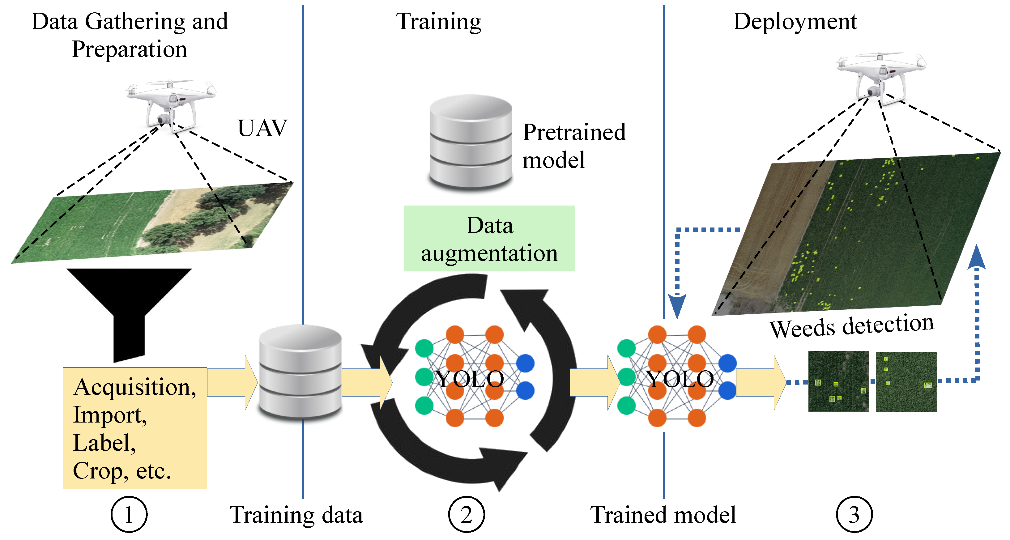
The working pipeline of this study for weed detection using the CP and LB datasets is described in Figure 1. The figure depicts the process of weed detection from raw weed images to final prediction. The Roboflow [49] tool labels the raw images of the dataset and changes the image format for the YOLOv7 detector. The YOLOv7 detector uses these labeled images for the training process. Finally, the trained model is applied to images never seen in training and identifies weeds as a final result through bounding boxes. In this work, the YOLOv7 model is used as is with no modification to the original implementation. Anyone can download the exploited version from the GIT repository to use it as we have [50]. The following subsections provide a detailed explanation of all modules of the YOLOv7 model and their use to solve the problem of weed detection.

3.1. You Only Look Once v7

YOLOv7 [25] is a recently released model after its predecessor, YOLOv6 [24]. YOLOv7 delivers highly enhanced and accurate object detection performance without increasing the computational and inference costs. It effectively outperforms other well-known object detectors by reducing about 40% of the parameters and 50% of the computation required for SOTA real-time object detection. This allows it to perform inferences more quickly with higher detection accuracy.

YOLOv7 delivers a faster and more robust network architecture that offers a more efficient feature integration approach, more precise object recognition performance, a more stable loss function, and an optimized assignment of label and model training efficiency. Consequently, in comparison with other DL models, YOLOv7 uses far less expensive computational hardware. On small datasets, it can be trained significantly more quickly without the use of pretrained weights.

In general, YOLO models perform object classification and detection simultaneously just by looking once at the given input image or video. Thus, the algorithm is called You Look Only Once. As shown in Figure 2, YOLO is a single-stage object detector with three important parts in its architecture: the backbone, neck, and head. The backbone is responsible for the extraction of features from the given input images, the neck mainly generates the feature pyramids, and the head performs the final detection as an output.

In the case of YOLOv7, the authors introduced many architectural changes, such as compound scaling, the extended efficient layer aggregation network (EELAN), a bag of freebies with planned and reparameterized convolution, coarseness for auxiliary loss, and fineness for lead loss.

3.1.1. Extended Efficient Layer Aggregation Network (EELAN)

The EELAN is the backbone of YOLOv7. By employing the technique of “expand, shuffle, and merge cardinality”, the EELAN architecture of YOLOv7 allows the model to learn more effectively while maintaining the original gradient route.

3.1.2. Compound Model Scaling for Concatenation-Based Models

The basic goal of model scaling is to modify important model characteristics to produce models that are suitable for various application requirements. For instance, model scaling can improve the model’s resolution, depth, and width. Different scaling parameters cannot be examined independently and must be taken into account together in conventional techniques using concatenation-based architectures (such as PlainNet or ResNet). For example, increasing the model depth will affect the ratio between a transition layer’s input and output channels, which may result in less usage of hardware by the model. Therefore, for a concatenation-based model, YOLOv7 presents compound scaling. The compound scaling approach allows the model to keep the properties that it had at the initial level and consequently keep the optimal design.

3.1.3. Planned Reparameterized Convolution

Reparameterization is a method for enhancing the model after training. It extends the training process but yields better inference outcomes. Model-level and module-level ensembles are the two types of reparametrization that are used to conclude the models. There is another kind of convolutional block called RepConv. RepConv is similar to Resnet except that it has two identity connections with a 1 × 1 filter in between. However, YOLOv7 uses RepConv (RepConvN) without an identity connection in its planned reparameterized architecture. The authors’ proposed idea was to prevent an identity connection when a convolutional layer with concatenation or a residual is used to replace the reparameterized convolution.

3.1.4. Coarseness for Auxiliary Loss and Fineness for Lead Loss

A head is one of the modules in the YOLO architecture which presents the predicted output of the model. As in Deep Supervision, YOLOv7 also consists of more than one head. The final output in the YOLOv7 model is generated by a lead head, and the auxiliary head is responsible for helping the training process in the middle layer.

A two-label assigner process is introduced, where the first is the lead head-guided label assigner. This is primarily calculated using the predicted outcomes of the lead head and the ground truth, which produce a soft label through an optimization process. Both the lead and auxiliary heads use these soft labels as the target training model. The soft labels produced by the lead head have a greater learning capacity, which is why they represent the distribution and correlation between the source and the target data. The second part is the coarse-to-fine lead head-guided label assigner. It also produces a soft label by using the predicted outcomes of the ground truth with the lead head. However, during the process, it produces two distinct collections of soft labels, referred to as the coarse and fine labels. The coarse label is produced by letting more grids be dealt with as positive targets, whereas the fine label is identical to the soft label produced by the lead head-guided label assigner. The significance of coarse and fine labels can be dynamically changed during training, owing to this approach.

3.2. Models and Parameters

To identify weeds using the LB and CP datasets, we used one of the SOTA YOLOv7 one-stage detectors and compared its performance with other one-stage detectors, such as YOLOv5 [23], YOLOv4 [22], and YOLOv3 [21], and two-stage detectors such as the Faster-RCNN [17]. To assist the training, all the YOLOv7 models were trained using transfer learning with the MS COCO dataset’s pretrained weights. The one-stage models used Darknet-53, R-50-C5, and VGG16 [21] as a backbone, and the two-stage models used different backbones, such as R-50 FPN, Rx-101 FPN, and R-101- FPN.

Table 1. Parameters used for training one-stage detector models such as YOLOv7, YOLOv5, YOLOv4, and YOLOv3.

Parameters	Values
Optimizers	Adam
Learning rate	Adam = $1\times {10}^{-3}$
Momentum	0.98
Learning decay	$1\times {10}^{-2}$
Pretrained	MS COCO dataset
Number of epochs	300

and

Table 2. Parameters used for training the YOLOvF and SSD models.

Parameters	YOLOvF	SSD
Optimizers	SGD	SGD
Learning rate	0.12	0.002
Momentum	0.9	0.9
Learning decay	0.0001	0.0005
Pretrained	resnet50-caffe	COCO
Number of epochs	300	300

describe the different parameters used during training for the one-stage models and the models which were used for comparison. In all the experiments reporting the results of the YOLOv7 model, we used Pytorch’s implementation of YOLOv7 as is, which anyone can download from the GIT [50] repository.

During experiments, training and testing were run on a Quadro RTX5000 GPU with 16 GB VRAM. For all the models, the batch size, which is the number of samples of images that are passed to the detector simultaneously, was equal to 16. During the training process, the model weights with the highest mAP on the validation set were used for testing each model. The intersection over union (IOU) threshold for validation and testing was 0.65. In this study, we performed different experiments: (1) the YOLOv7 detectors were applied to the LB dataset to locate and identify the weeds; (2) we used the YOLOv7 pretrained weight of the LB dataset obtained after the first experiment and applied it over the CP dataset to identify weeds; (3) the YOLOv7 detector with all variants was used to locate and identify the weeds using the normal CP dataset; (4) for comparison purposes, we applied the Single-Shot Detector (SSD) [51], YOLOv3 [21], and YOLOvF [52] detectors using the CP dataset; and (5) we used an augmented CP dataset for the identification of weeds using YOLOv7 detectors. The results of the above-mentioned experiments are given in Section 5.

4. Dataset

To examine the behavior of the YOLO model family, when used to solve the problem of the detection of weeds, we used two datasets: (1) the Lincoln Beet (LB) crop dataset [33] available in the literature, which we used to compare our results with those already published, and (2) the Chicory Plant (CP) crop dataset, a very complex dataset generated from UAV acquisition in real case field conditions, which was built in this work specifically to study the behavior of YOLOv7 as a solution to the weed detection problem for UAV data.

4.1. Lincoln Beet (LB) Dataset

The images in the LB dataset came from the fields where sugar beets were produced for commercial purposes, and all the images included beets and harmful weeds along with their respective bounding boxes. The LB dataset contains 4405 images of 1902 × 1080 pixels. The LB dataset images were taken from recorded videos of sugar beet fields at various times. These images were collected from May to June 2021, when each sugar beet field was scanned at least four times a week to record weeds at various development stages. During video recording, the camera was roughly 50 cm away from the ground during each scanning session. There were two cameras utilized: one with a 12-megapixel sensor, an f1.6 aperture, and a 26 mm focal length and the other with a 64 megapixel sensor, an f2.0 aperture, and a 29 mm focal length. The images from both cameras were originally 2160 × 3840 pixels in size. The fields utilized for the LB dataset are located in Lincoln, UK at various sites with different soil types, plant distributions, and weed species.

Table 3. Characteristics of the Lincoln Beet (LB) and Chicory Plant (CP) datasets.

	LB Dataset	CP Dataset
Number of images	4402	3373
Number of bounding boxes	39,246	12,113
Average weeds per picture	5.190	3.561
Total number of weeds	22,847	12,113
Number of sugar beets	16,399	N/A

shows the characteristics of the LB dataset.

4.2. Chicory Plant (CP) Dataset

The experimental site (50°30${}^{\prime }$N–50°31${}^{\prime }$N; 4°44${}^{\prime }$E–4°45${}^{\prime }$E) was an agricultural field of about 5 ha in central Belgium with a temperate climate. The soil type was luvisol cultivated with chicory (Cichorium intybus subsp. intybus convar. Sativum). We conducted the UAV campaigns from April to August throughout the 2018 cropping season. A DJI phantom4 pro (DJI, Nanshan, Shenzhen, China) was used to capture images over the CP fields. The flying altitude of the UAV was 65 m above ground level, with an airspeed of 5 m/s and 75% sideways and 85% forward image overlap. The UAV flights were executed at the nadir with an 84° field of view and 5472 × 3648 pixel size RGB images, resulting in very high-resolution UAV images with a ground sampling distance of 1.8 cm. One main advantage of RGB imagery is its ease of operation and image processing chains. Furthermore, RGB images offer a sharper representation of the surface details, which is an important constraint in research focusing on object-based image analysis such as in the present study. The UAV images of the CP dataset contain highly detailed spatial surface characteristics about either green or senescent chicory plants alongside weeds, crop residues, and bare soil. Mercurialis annua (French mercury) is the weed species of the Euphorbiaceae spurge family present in the field in the present study. This is a rather common wheat species within the cereal fields of European countries such as Belgium [53].

After capturing the images, appropriate data handling was requested to create the CP dataset to be exploited in YOLO model training and to test the detection performances. A detailed explanation on how the images were preprocessed and labeled is provided in the Supplementary Materials (S1). To properly annotate (physically drawing bounding boxes) and label (defining the target category) the UAV-acquired images, the Roboflow application was used [49,54]. It is worth stating that during the green-up phase of chicory plants, most of the weed objects were still rather small to be properly identified in the acquired images. As such, in this paper, we focused solely on the UAV images for August, in which the weeds are well-developed. However, it was still challenging to purely discriminate weeds from senescent plants. To address the aforementioned difficulties, we proposed the three following rules to classify an object as a weed: (1) the color of the object to differentiate diseased and senescent leaves from weeds, (2) the shape of the object to differentiate crop residues from weeds, and (3) the height of the object to differentiate bare soil (e.g., inter-rows) from weeds.

Figure 3 provides an example of one image used to create the CP dataset. Weeds (yellow boxes) were identified according the previously mentioned criteria and using Roboflow’s online tools. Each original image was then cut using a custom-written Python script into smaller patches (i.e., blue boxes) to be processed by the neural network. Only the patches containing weeds were extracted and used to generate the CP dataset. We generated two versions of the CP dataset: the normal CP dataset and an augmented CP dataset (see Supplementary Materials (S1) for details).

The LB dataset contains two classes named “sugar beet” and “weed”, while the CP dataset contains only one class for detection, named “weeds”. Both datasets were randomly split into test, validation, and training sets with 20%, 10%, and 70% of all the images, respectively. The images and annotations were cropped into two distinct sizes—416 × 416 pixels and 640 × 640 pixels—while maintaining the width/height ratio in order to test the techniques under various image resolutions.

5. Results

We assessed the trained models in various ways across the LB and CP datasets. Overall, the YOLOv7 models showed significant training results in terms of conventional metrics such as mAP, recall, and precision.

Table 4. Performance of the proposed YOLOv7 model, trained for 300 epochs on the LB dataset and compared to other models. The best results are highlighted in bold.

Model	Backbone	mAP Score	mAP Suger	mAP Weed
YOLOv7	DN-53	61.0	74.1	48.0
YOLOv5m	DN-53	51.0	67.5	34.6
YOLOv4	DN-53	41.2	59.5	23.0
YOLOv3	DN-53	50.4	66.3	34.6
F-RCNN	R-50 FPN	42.4	62.2	22.6
F-RCNN	R-101 FPN	42.2	62.2	22.3
F-RCNN	Rx-101 FPN	43.2	62.8	23.6
SSD	VGG-16 Bi-Real	37.4	54	20.8

shows the performance of the proposed YOLOv7 model for the LB dataset, and the best results are highlighted in bold. After 200 epochs during the training of the LB dataset, the results revealed that the performance leveled off with the existing LB dataset results. Therefore, 300 epochs were sufficient for the LB dataset training process. It can be observed from Table 4 that YOLOv7 outperformed the existing one-stage and two-stage models [33], and it achieved the highest mAP values for weed and sugar beet detection. It improved the accuracy from 51.0% to 61.0% compared with YOLOv5. It also enhanced the results from 67.5% to 74.1% and from 34.6% to 48.0% in the case of mAP for sugar beets and weeds, respectively.

For the weed extraction, we performed testing over the CP test set using a YOLOv7 model pretrained on the LB dataset.

Table 5. Test results on the CP test set using the YOLOv7 model pretrained on the LB dataset.

Class	Images	Labels	P	R	mAP@.5	mAP@.5:.95
All	501	1180	7.83 $\times {10}^{-5}$	0.000847	5.31 $\times {10}^{-7}$	5.31 $\times {10}^{-8}$
Weeds	501	1180	7.83 $\times {10}^{-5}$	0.000847	5.31 $\times {10}^{-7}$	5.31 $\times {10}^{-8}$

illustrates the testing outputs obtained on the CP test set. During this testing, as we can see in Figure 4, the YOLOv7 model pretrained on LB was not able to predict the weeds’ bounding boxes from the CP test set images. In many images of the CP dataset, the pretrained model predicted some very large bounding boxes compared with the size of the plants present in the images. This situation was due to the significant difference between the two datasets. The model was trained to recognize weeds from the LB dataset, in which the plants are all seen at close range as well as spaced apart, and the underlying ground is almost always visible between the plants. In the CP dataset, on the other hand, the plants are always seen from a greater distance and are all close together. This difference explains the very large bounding boxes, where the content was a continuous but uninterrupted expanse of chicory plants and weeds wherever the underlying ground was not visible.

It is also clear from Table 5 that the YOLOv7 model trained on the LB dataset failed to detect weeds from the CP dataset and showed inappropriate precision, recall, and mAP results in this regard.

For the CP dataset, the experimental results of all the YOLOv7 variants are given in

Table 6. Performance of all the YOLOv7 variants for the CP dataset. Best results are in bold.

Model	Precision	Recall	mAP@ 0.5 Score	mAP@0.5:0.95 Score
YOLOv7-tiny	57.6	58.3	55.8	17.9
YOLOv7m	55.2	60.9	56.3	18.5
YOLOv7-x	59.3	58.1	56.6	18.5
YOLOv7-w6	55.3	62.1	56.5	18.5
YOLOv7-e6	59.2	57.0	56.0	17.9
YOLOv7-e6e	57.1	58.8	55.3	18.1
YOLOv7-d6	61.3	54.8	55.0	18.1

, where the batch size and the number of epochs were 16 and 300, respectively. We can see from Table 6 that YOLOv7-d6 achieved the highest precision score compared with the other YOLOv7 variants.

Furthermore, YOLOv7-w6 also outperformed the other YOLOv7 variants by obtaining 62.1% recall and a 65.6% mAP score. However, the YOLOv7m, YOLOv7-X, and YOLOv7-w6 variants achieved the same 18.5% scores in the case of mAP@0.5:0.95. For a fair comparison of the YOLOv7 model, it can be seen in

Table 7. Performance comparison for object detectors with CP dataset.

Models	Backbone	Recall	mAP Weed
YOLOv7	DarkNet-53	58.1	56.6
YOLOv3	DarkNet-53	31.3	22.18
YOLOvF	R-50-C5	54.6	24.97
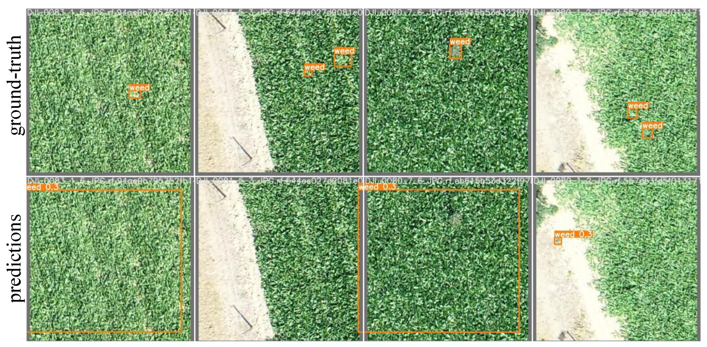
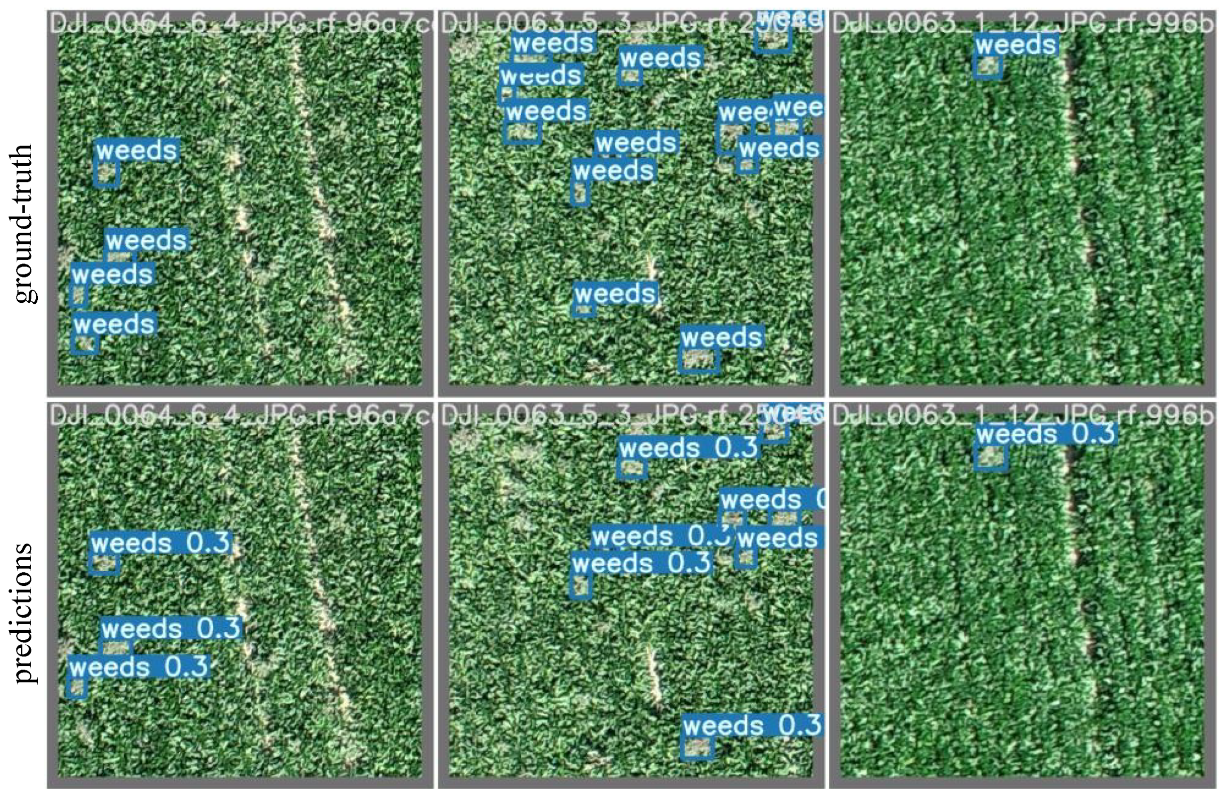
SSD	VGG16	75.3	23.74

that YOLOv7 obtained a 56.6% mAP score and successfully outperformed the existing detectors, such as SSD, YOLOv3, and YOLOvF, using the CP dataset. However, the SSD detector showed 75.3% higher results than YOLOv7, YOLOv3, and YOLOvF in terms of the recall evaluation metric. Furthermore, for the results of the augmented CP dataset, all the YOLOv7 variants showed lower results than the normal CP dataset. YOLOv7m and YOLOv7-e6 achieved only 50.0% and 49.0% mAP scores, respectively. However, only the YOLOv7-e6 variants achieved the highest 66.0% precision score over the augmented CP dataset. Some examples of weed detection are shown in Figure 5 for the CP dataset and Figure 6 for the LB dataset. In these examples of detections obtained with YOLOv7 on the test images, it was possible to analyze the behavior of the model for all the classes of the two datasets. Further analysis and discussion of the experimental results are given in Section 5.

Discussion

Deep Learning is increasingly gaining popularity in the research community for applications in precision agriculture, such as weed control. Farmers can use more effective weed management techniques by identifying the weeds in a field. Researchers are getting more concerned about image classification, using CNNs to identify weeds. However, it can be difficult to reliably detect multiple weeds in images when using image classification, as it can only detect individual objects using UAV images taken at high altitudes. However, the detection of weeds is of significant importance, as weed location within fields is required to ensure fruitful weed management. Therefore, in this work, we performed object detection for the identification and location of multiple weeds using UAV-captured images. Farmers can target the areas of the crops where weeds are prevalent for the application of herbicides, reducing expenses, minimizing adverse effects on the environment, and improving crop quality.

Research for weed identification has been scarce in the literature. This is mainly due to the scarcity of the required annotated datasets for weed detection. The dataset is the core of a DL model, as without a dataset, we are unable to train the models, and all the automation and modern research will be in vain. A large, efficient, and suitable weed dataset is always a key factor for the success of DL models in weed management. All the existing agricultural datasets contain various crop images for different purposes. We cannot use a pretrained model of any specific weed dataset to recognize weeds from our proposed CP dataset. To verify this, we used a model pretrained on the LB weed dataset to detect weeds from a test set of the CP dataset. This yielded poor results, as we can see in Table 5 and Figure 4, and this became the motivation to propose a new weed dataset whose trained model can detect relevant weeds in UAV-based RGB images. Construction of a weed dataset is a tedious task, as annotations and labeling the images takes human effort, is time-consuming, and requires weed experts to double-check and visualize the dataset to assure its quality. For that purpose, we used chicory plant fields at research locations in Belgium to capture the images. A DGI phantom4 UAV was used to acquire RGB images. Furthermore, these RGB images were annotated and labeled by the Roboflow application to generate a suitable format for training of the YOLOv7 model. This study makes a distinctive contribution to the scientific community in weed recognition and control by introducing and publishing a novel weed dataset with almost 12,113 bounding boxes.

In this work, weeds were identified and located using a SOTA Deep Learning-based object detector. Although many different CNN-based algorithms may be used to achieve object detection, the YOLOv7 detector was adopted because of the few parameters required for rapid training, inference speed, and detection accuracy scores for quick and precise weed identification and localization. This detector was highly useful for identifying multiple weed objects, especially when the nearby emerging crops were of a similar size and color.

All the YOLOv7 models delivered visually appealing predictions with a diverse background and with heavily populated weeds. Overall, these findings demonstrate that the chosen YOLO object detectors were effective for the LB dataset and the newly introduced CP dataset for weed detection. The YOLOv7 model efficiently performed weed detection using the LB dataset, and its results outperformed the existing outcomes of the LB dataset [33]. In a comparison of the outputs of YOLOv7 using the CP dataset with the other detectors, YOLOv7 ranked first among the SSD, YOLOv3, and YOLOvF models. It achieved a higher mAP score and outperformed the other detectors by a high margin. However, the SSD model obtained higher recall in comparison with YOLOv7, YOLOv3 and YOLOvF. In the case of the augmented CP dataset, all the variants of YOLOv7 showed slightly lower results using the augmented CP dataset than the normal CP dataset. This was due to the already implemented data augmentation techniques of the YOLOv7 detector, as YOLOv7 is heavily used in built augmentation techniques during experiments, such as flip, mosaic, PasteIn, and cutout. In addition, YOLOv7-e6 showed improved results and achieved 66% accuracy using the augmented CP dataset and outperformed all YOLOv7 variants’ performances over the normal CP dataset. Therefore, there is no need to add augmentation techniques to the CP dataset. Additionally, a favourable comparison was made between the detection accuracy of YOLOv7 and the earlier weed identification studies. We know that the CP dataset can be extended to other weed types, different crops, and different growth stages for weeds and crops, but in conclusion, we believe that the proposed CP dataset can be considered a good starting benchmark for all models trained for weed detection from UAV images. This is because the RGB images acquired by UAVs have similar characteristics for acquisition height with respect to the ground. Moreover, many other crops have characteristics similar to those of the chicory plants proposed in this work. For this reason, we believe that the CP dataset can be used to pretrain detection models that can be used in other regions and on other crop types.

6. Conclusions

Weed detection is a necessary step for CV systems to accurately locate weeds. Deep neural networks, when trained on a huge, carefully annotated weed dataset, are the foundation for an efficient weed detection system. We address the most detailed dataset for weed detection relevant to chicory plant crops. This work demonstrated that training an object detector such as YOLOv7, trained on an image dataset such as the CP dataset proposed in this work, can achieve efficient results for automatic weed detection. Additionally, this study has demonstrated that it is possible to train an object detection model with an acceptable level of detection accuracy using high-resolution RGB data from UAVs. The proposed CP dataset consists of 3373 images with a total of 12,113 annotation boxes acquired under various field conditions, which is freely downloadable from the web [34]. In the case of the CP dataset, the YOLOv7-m, YOLOv7-x, and YOLOv7-w6 models achieved the same 18.5% mAP@0.5:0.95 scores, while YOLOv7-x outperformed the other YOLOv7 variants and showed a 56.6% mAP@0.5 score. Furthermore, the YOLOv7-w6 and YOLOv7-d6 models surpassed the other variants and obtained the best 62.1% and 61.3% recall and precision scores, respectively. The YOLOv7 model also outperformed the existing results of the LB dataset by margins of 13.4%, 6.6%, and 10% in terms of the mAP for weeds, mAP for sugar beets, and total mAP, respectively. Overall, the YOLOv7-based detection models performed well against the existing single-stage and two-stage detectors, such as YOLOv5, YOLOv4, the RCNN, and the FRCNN, in terms of detection accuracy, and YOLOv7 showed better results than YOLOv5 in the LB dataset in terms of the mAP score. In the future, we will consider weed detection outcomes on UAV-acquired images at different heights above ground level.